Photocell Optimisation Using Dark State Protection
Abstract
Conventional photocells suffer a fundamental efficiency threshold imposed by the principle of detailed balance, reflecting the fact that good absorbers must necessarily also be fast emitters. This limitation can be overcome by ‘parking’ the energy of an absorbed photon in a dark state which neither absorbs nor emits light. Here we argue that suitable dark states occur naturally as a consequence of the dipole-dipole interaction between two proximal optical dipoles for a wide range of realistic molecular dimers. We develop an intuitive model of a photocell comprising two light-absorbing molecules coupled to an idealised reaction centre, showing asymmetric dimers are capable of providing a significant enhancement of light-to-current conversion under ambient conditions. We conclude by describing a roadmap for identifying suitable molecular dimers for demonstrating this effect by screening a very large set of possible candidate molecules.
Keywords:
Suggested keywordspacs
Valid PACS appear hereI Introduction
The operation of a solar energy harvesting device can be enhanced by clever design of a nanoscopic, quantum mechanical system [1]. Though thermodynamical considerations lead to the famous Shockley-Queisser efficiency limit for classical photocell devices [2], the ‘detailed balance’ underlying this limit can be broken by careful use of quantum interference. In particular, by carefully tailoring the interactions between two [3, 4] or more [5, 6] idealized and identical two-level energy absorbers, it is possible to prevent the re-emission of absorbed light by arranging that excitations end up in ‘dark’ – i.e. optically inaccessible – states. This allows the energy to be dissipated across a target load, rather than dissipated via spontaneous emission.
It is conjectured that nature already exploits quantum-mechanical properties in order to increase the light-harvesting efficiency of photosynthesis [7]. The most well studied system in this context is the FMO complex [8], which connects the antenna to the reaction centre in the light harvesting apparatus of green sulfur bacteria. It consists of seven (or eight [9]) bacteriochlorophyll (BChl a) molecules that are held in place by a messy protein scaffold, and surrounded by water at room temperature, resulting in non-identical BChl excitation energies. True quantum effects may seem unlikely in the ‘hot and wet’ conditions of such systems. However, the observation of quantum coherent beats in experimentally measured two-dimensional electronic spectroscopy suggests otherwise [10, 11, 12, 13, 14, 15, 16].
A good definition of the term efficiency is key to quantifying a quantum advantage. One such measure is the energy transfer efficiency, i.e. the probability of an excitation reaching the target electron acceptor after starting from a spatially localised state [17, 18, 19], but this does not capture all aspects of the process. An alternative approach is placing a system between two electrodes, and measuring the current through them[20, 21, 22, 23]. Dorfman et al. proposed a different canonical measure [1]: They consider the entire cycle, from absorbing a photon to extracting work, as a quantum heat engine (QHE). Procedurally, they abstract the electron acceptor to become a two-level ‘trap’, in which transferred electrons ‘fill’ the excited state before the action of driving a load resistor is mimicked by decay to the lower level of the trap. This gives a straightforward way of defining the power and the efficiency of the heat engine. In this picture, Fano interference may boost the photocurrent by 27% over that of a classical cell. Subsequently, Creatore et al. [3] reported an efficiency gain of 35% by introducing the different effect of dark-state protection using two identical dipole-coupled emitters. Further gains become possible for more than two chromophores [5, 6].

II Model
In this Letter, we use the QHE framework to determine whether a quantum advantage is achievable in non-idealized situations typical of real devices and conditions more closely resembling the photosynthetic apparatus. In particular, we consider a light harvesting device where the two constituent chromophores are not identical. Surprisingly, we will find that under realistic constraints an ‘asymmetric’ dimer may even significantly outperform previously studied systems. Presenting several example molecules that would be highly efficient light harvesters according to our model, we argue that the number of conceivable molecular dimers with a quantum advantage is vast.
We now introduce a general framework that will allow us to define three specific models shortly. We consider two, generally different, light-absorbing molecules with dipolar coupling. There is a further coupling to an abstracted reaction center ‘trap’, modelled as a two level system , with corresponding energies , following Ref. 1. An excitation absorbed by the molecules can be incoherently transferred into the reaction centre via a phonon-assisted process. In what follows we restrict the dynamics to the subspace with one or zero excitations across the entire system: this approximation is valid since in realistic configurations inspired by natural photosynthetic systems, the average excitation number is very small ( for an energy gap of eV and sunlight temperature of 6000 K). Since photoexcitation is very rare, once captured it is paramount to prevent spontaneous emission back into the environment. Hence, access to a dark state, i.e. a state that is decoupled from the photon field and thus not susceptible to spontaneous emission decay, can enhance the engine’s efficiency. By Kasha’s rule re-emission of absorbed photons will be dominated by the lowest excited state, motivating our approach of only considering a single excited level per chromophore.
We denote the excited states in the molecules as with energies , , respectively, and the ground state as with energy , and is the dipolar coupling between the molecules. The Hamiltonian of the system is thus of dimension five and given by (see Fig. 2)
| (1) | ||||
| (2) |
In the second equation, are the usual eigenstates diagonalising the subspace spanned by .
In addition to the bare system we also have the solar photonic bath at K, which can induce spontaneous and stimulated transitions and . Further, each molecule is embedded in its own local environment of vibrational modes, treated as infinite phonon baths at room temperature K. A generic spin boson type interaction between excitonic states and phonon modes yields transitions between the energy eigenstates [24]. Further, we include the reaction center decay with rate , and some leakage between and with rate . The interaction Hamiltonian is thus
| (3) |
Here , and are operators of the coupling to the different environments: are dipole operators, and the rest are phonon operators 11 1 See Appendix B.
Applying a standard Born-Markov procedure [26] we arrive at a set of Pauli master equations 11footnotemark: 1 :
| (4) |
Here is a vector of the populations in the diagonal basis of the system, and is a matrix of the different rates, respecting detailed balance for photon and phonon baths independently. Resulting transition rates are depicted in Fig. 2 and conservation of total population imposes the additional constraint . We give the explicit entries of in Appendix B.3, and also show that this rate equation approach is valid by direct comparison with the full Bloch-Redfield equations.

Utilising the concept of a photochemical voltage [27], we attribute an effective current and voltage to the reaction center [1]:
| (5) |
Following Refs. 1, 3, 4, 5, 28 we now consider quantity as a measure of the power generated by the system. Here is the (cold) phonon temperature, the Boltzmann constant, and the electron charge. In the absence of sunlight, the system thermalizes to the phonon bath temperature, and the voltage vanishes. Thus is a measure of the deviation from the thermal state with temperature . We are interested in the steady-state power output, which is found by setting the LHS of Eq. (4) to zero and solving the resulting simultaneous algebraic equations.
Our Hamiltonian is static, and so there is no cycle as there would be for conventional quantum heat engines [29, 30, 31]; our device rather relies on heat flowing through the reaction centre to produce work [32, 33, 34]. Henceforth, we adopt the maximal achievable steady state power as our measure of efficiency: we treat the reaction centre as a black box optimizing its to generate maximal power (keeping all other parameters fixed). For a representative example of the behaviour of and as a function of see Fig. 9.
We now define the three specific models which we shall compare. These have contrasting molecular geometries and are depicted in Fig. 1. First, the independent model has two identical light harvesting molecules that are not directly coupled to one another whilst each is independently coupled to the reaction centre. Specifically ; represent the coupling to different phonon baths, and . Further, we let , . This model does not exhibit dark state protection and serves as a benchmark for the other models.
Second, the symmetric model mirrors that described in Ref. 3 and consists of two identical, directly coupled molecules: , , and . This arrangement leads to a dark and bright state, and respectively, with and . The molecules couple to the reaction center in anti-phase [3], rendering . We discuss deviations from this idealized scenario in Appendix B.
Finally, the asymmetric model is the main focus of our Letter. It comprises two non-identical molecules with different dipole moments where represents the asymmetry. The dark(er) state has a larger overlap with molecule 1, which we imagine closer to the reaction center, and we assume molecule 2 only has negligibly small reaction center coupling (). We believe that this configuration should be easier to realise than the symmetric model, while allowing engineering of the energy gap . For flat spectral densities of the environments around the transition frequencies, we find this asymmetric model exhibits a fully dark state, provided that , , and satisfy the relation:
| (6) |
Explicit rates for this system are given in Appendix B.3. Whether or not is indeed fully dark, we can express the resulting total excitation rate through an angle :
| (7) | ||||
| (8) |
Thus , and in the presence of a completely dark state.
Several mechanisms may cause deviation from a fully dark state in both coupled models: First, different local environments would generally entail differing reorganization energy shifts and thus excitation energies. For example, the FMO complex consists of seven identical BChl units, embedded in a protein scaffolding, resulting in on-site energies spanning a range of 25 meV [10]. Second, the two dipoles may be at an angle instead of parallel [3], breaking the interference needed for a completely dark state. Third, the coherent coupling depends on both the distance between the two molecules, and the angle : , where is the coupling with parallel dipoles. Taking all this into account we get in the general case, i.e. for all models,
| (9) |
with being the Rabi frequency of the bare system between sites 1 and 2. Further discussion about deviation from the fully dark state, and details on the coupling to the reaction centre are given Appendix B.
The performance of the (a)symmetric relative to the independent models will be assessed by using our simulations to determine the ratio of the respective maximum powers, found by varying in each case [see Eq. (5)]. For a fair comparison, we keep , , and equal across all three models.
III Numerical results
Fig. 3 presents the enhancement achievable by dark-state protection. Here we have optimized as well as with all other parameters fixed. We also constrain to below meV as an upper limit of realistic coupling strength. For the asymmetric model the dark state criterion, Eq. 6, informs an appropriate dipole asymmetry for a given value of . Quantum enhancement is only possible when the transfer into the reaction center is relatively slow and constitutes a bottleneck in the cycle. In the limit of an upper bound to the enhancement emerges. Within a reasonable parameter range this limit grows with increasing for the symmetric and with for the asymmetric case. As strong coupling is harder to realise than site energy mismatch, asymmetric dimers might more easily achieve high performance. We note that deeper into the slow transfer limit the potential enhancement factors can significantly exceed the values of up to 50% reported by Refs. 1, 3, 5. By contrast, for fast transfer rates dark-state protection offers no advantage: absorbing photons at an energy higher than the extraction energy (i.e. at reduced thermal photon occupancy), combined with , is now detrimental.
Fig. 4 shows the relative power enhancements of the asymmetric model as a function of the energy difference and of the coupling . We also plot the equivalent enhancement given by the symmetric model, and show there is a parameter regime, with boundaries marked by a black line, for which the asymmetric model outperforms the symmetric one. The asymmetric model displays a peak power enhancement at finite coupling and energy difference. This happens for two reasons: First, in the regime , the rate is non-negligible, and so the dark state is not protected. Second, if , the rate becomes negligible, and the dark state is rarely populated. Note that in the limit , the asymmetric model gives a smaller power than the independent benchmark. This is because we set for the asymmetric model, effectively making it a single antenna setup benchmarked against two antennae. We examine further realistic imperfections, including the presence of additional dephasing mechanisms, in Appendix B.

IV Candidate molecules for realizing the asymmetric model
To assess the feasibility of generating suitable asymmetric molecules for power enhancement, we use a library containing quantum-chemically predicted properties of organic light-emitting diode molecules [35] to identify systems that minimize in Eq. (9). Appendix A provides a full account of how quantum chemical calculations lead to promising molecular dimer candidates through a rigorous multistage process. Our donor candidates feature strongly allowed optical transitions ( of 3.5 atomic units) and site energies between 3.5 to 2.5 eV to optimally absorb sunlight. As required by the model, acceptable acceptor compounds must have and possess lower transition dipole moments with to deliver . For simplicity, we assume fully aligned transition dipole moments and center-to-center distances between donor and acceptor moieties of 1 nm (approximately corresponding to the size of a small aromatic bridging group), resulting in an inter-site coupling of up to 15 meV. Importantly, we analyse the properties of our dimers for both ground and excited state equilibrium geometry to identify systems whose relevant properties are robust to vibrational relaxation effects accompanying optical absorption and emission.
The predicted properties of a selection of molecular pairs are reported in Table 1 of Appendix A and an illustration of some molecules is shown in Fig. 5. These examples provide evidence that the chemical regime required for dark-state protection is readily available in ordinary molecular systems. A full implementation of the proposed model would also require an additional molecular system to act as a trap, as well as control over orientation and distance between donor and acceptor. Whereas the chemical synthesis of such a complex structure is challenging, our results show that matching fundamental components for such a system is entirely feasible.
V Summary and Conclusions
In conclusion, we have presented a general model of light absorption by an asymmetric pair of coupled chromophores, finding that it can outperform both the symmetric dimer and a pair of independent molecules in realistic parameter regimes of operation for a solar cell device. Not relying on identically matched coupled chromophores, this approach is more robust to deviations from the delicate conditions required by its symmetric counterpart. Moreover, we have shown that an abundance of real pairs of molecules have the required asymmetric properties, and indeed, such asymmetry is an integral part of natural photosynthetic systems.
The reason our asymmetric model works so well is that it enables arbitrarily large energy gaps between the bright and dark states, thus preventing phonon-assisted promotion from the dark to the bright state. In the regime where excitations are rare and the transfer into the reaction center is very slow, this translates into better protection of the excitations, thus increasing the overall efficiency of the device.
Acknowledgements.
We thank Alex Chin, Ahsan Nazir, Simon Benjamin, Alán Aspuru-Guzik, and Jorge Aguilera-Iparraguirre for stimulating discussions. This work was supported by the Leverhulme Trust (RPG-080). EMG is supported by the Royal Society of Edinburgh / Scottish Government. RGB thanks Samsung Advanced Institute of Technology for funding. AF thanks the Anglo-Israeli association and the Anglo-Jewish association for funding.Appendix A Molecular dimers candidates
In the following we discuss a possible roadmap towards finding candidate dimer systems based on pairs of real molecules, which are predicted to display the desired dark-state protection effect. Our pool of molecules consists of a database listing 500,000 viable organic dye molecules. Their site energies and transition dipole moments were calculated at the TD-DFT B3LYP/6-31G(d) level of theory on molecular geometries optimized at the B3LYP/6-31G(d) level.[35]
As a starting point in our endeavour to identify potential dimer candidates, we survey the relevant optical properties of individual molecules. Figure. 5 shows the distribution of absorption energy vs optical dipole strength across all molecules in the database.

Recognising that vibronic effects are usually important in molecular systems, we have calculated the effect of geometric relaxation on a selection of 2,000 molecules by optimizing the molecular geometries of their lowest excited state at the TD-DFT B3LYP/6-31G(d) level of theory. In Fig. 6 we survey the relevant optical properties of this reduced sample. We plot the absorption energy as a function of optical dipole strength (upper left panel), the relative difference in dipole strength between absorption and emission (upper right panel), and the Stokes shift as a function of dipole strength and transition energy, respectively, (lower panels).
Of relevance to our scheme, we note there is an abundance of molecules with absorption energies in the 2.5-3.5 eV bracket — i.e., near the power maximum in the spectrum of sunlight — and that these molecules possess a varying degree of dipole strength. There are also a sizeable number of candidates with relatively low Stokes shift, mainly appearing in two clusters with comparatively strong and weak optical dipoles. Finally, candidates exist for which there is only a small difference in the dipole moments of absorption and emission, consistent with dipoles that have little dependence on vibronic coupling, suggesting that the nature of the relevant states will not change significantly with geometrical relaxation.


We now attempt to pair up molecules according to whether they show promise for displaying dark-state behaviour. For this purpose the donor and acceptor are assumed to be coupled via point dipole coupling of their lowest local excited states. For computational ease of screening the still large set of candidates, we base our estimate of the Förster coupling on the oscillator strength and transition energy of the absorption transition (S0). The histograms displayed in Fig. 7 report the density of suitable donor (or acceptor) partners in the database for a selection of 16 given acceptors (or donors) with a wide range of properties. As shown, a very large number of potential partner molecules with a high level of predicted dark state protection () exists in the majority of all cases considered.


To take a further step, we report a selection of 26 candidate chromophore pairs which are expected to be suitable for dark-state protection according to the predicted properties on the ground state equilibrium geometry (all rows in Table 1). These 26 candidates were obtained as combinations of the 6 donor and 20 acceptor molecules highlighted in Figs. 5 and 6. For these candidates we also calculate the emission properties, based on the excited state equilibrium geometry (results again in Table 1). This shows that not all pairs can be expected to be fully characterised by our simpler initial approach: Some molecules, particularly acceptors, have high vibronic coupling and experience large changes in both site energy and transition dipole upon excitation.
To screen further, we therefore select the six pairs with the overall most favourable values for across both excited and ground geometries. These highly promising candidate pairs are printed in rows A-F of Table 1, combining a pronounced dark-state both from the S0 and the S1 transition. No large-scale vibronic effects, such as state reordering are observed for the intermediate geometries for these pairs. We believe these dimer candidates would be excellent candidates for full experimental and/or ab-initio computational characterisation, as in intermediate goal on route to a full experimental implementation of our proposed scheme.
We note that throughout our process of narrowing down the field, we have at several stages had to reduce the pool of candidates by random selection, so our final list of six candidates will likely only be a tiny fraction of interesting dimer combinations existing in the full space of the database. Further, fluorescent dyes, such as cyanine or BODIPY derivatives were not explored in this particular dataset, but are also expected to produce species with large transition dipole moment at arbitrary absorption energies.
| # | Q | ||||||||||||||
|---|---|---|---|---|---|---|---|---|---|---|---|---|---|---|---|
| 1 | 2.73 | 3.54 | 2.45 | 3.32 | 2.61 | 0.94 | 1.97 | 0.06 | 0.27 | 0.02 | 0.013 | 0.012 | 0.044 | 0.000 | 1.41 |
| 2 | 2.73 | 3.54 | 2.45 | 3.32 | 2.63 | 1.02 | 2.00 | 0.17 | 0.29 | 0.05 | 0.015 | 0.013 | 0.047 | 0.001 | 1.45 |
| 3 | 2.93 | 3.52 | 2.56 | 4.13 | 2.82 | 0.90 | 2.18 | 0.00 | 0.26 | 0.00 | 0.013 | 0.018 | 0.038 | 0.001 | 1.45 |
| 4 | 2.93 | 3.52 | 2.56 | 4.13 | 2.82 | 1.09 | 2.43 | 0.93 | 0.31 | 0.23 | 0.015 | 0.021 | 0.055 | 0.020 | 1.43 |
| 5 | 2.93 | 3.52 | 2.56 | 4.13 | 2.81 | 1.11 | 2.17 | 0.04 | 0.32 | 0.01 | 0.016 | 0.022 | 0.060 | 0.000 | 1.40 |
| 6 | 2.90 | 3.52 | 2.44 | 3.29 | 2.80 | 0.89 | 2.16 | 0.04 | 0.25 | 0.01 | 0.013 | 0.011 | 0.035 | 0.000 | 1.47 |
| 7 | 2.90 | 3.52 | 2.44 | 3.29 | 2.78 | 0.87 | 2.17 | 0.06 | 0.25 | 0.02 | 0.012 | 0.011 | 0.037 | 0.000 | 1.44 |
| 8 | 2.90 | 3.52 | 2.44 | 3.29 | 2.78 | 0.89 | 2.17 | 0.37 | 0.25 | 0.11 | 0.013 | 0.011 | 0.038 | 0.008 | 1.44 |
| 9 | 3.04 | 3.45 | 2.70 | 3.33 | 2.94 | 0.92 | 2.37 | 0.11 | 0.27 | 0.03 | 0.013 | 0.012 | 0.040 | 0.000 | 1.46 |
| 10 | 2.94 | 3.48 | 2.65 | 3.52 | 2.84 | 0.74 | 2.36 | 0.38 | 0.21 | 0.11 | 0.010 | 0.011 | 0.026 | 0.008 | 1.47 |
| 11 | 2.94 | 3.48 | 2.65 | 3.52 | 2.82 | 0.90 | 2.18 | 0.00 | 0.26 | 0.00 | 0.013 | 0.013 | 0.041 | 0.000 | 1.43 |
| 12 | 2.94 | 3.48 | 2.65 | 3.52 | 2.82 | 0.97 | 2.27 | 1.20 | 0.28 | 0.34 | 0.014 | 0.014 | 0.049 | 0.103 | 1.41 |
| 13 | 2.94 | 3.48 | 2.65 | 3.52 | 2.81 | 1.11 | 2.17 | 0.04 | 0.32 | 0.01 | 0.016 | 0.016 | 0.065 | 0.000 | 1.38 |
| 14 | 2.80 | 3.57 | 2.23 | 1.49 | 2.68 | 0.86 | 2.07 | 0.04 | 0.24 | 0.03 | 0.012 | 0.002 | 0.035 | 0.001 | 1.44 |
| 15 | 2.80 | 3.57 | 2.23 | 1.49 | 2.66 | 0.98 | 2.20 | 0.58 | 0.28 | 0.39 | 0.014 | 0.002 | 0.049 | 0.117 | 1.36 |
| 16 | 2.80 | 3.57 | 2.23 | 1.49 | 2.68 | 1.06 | 2.08 | 0.56 | 0.30 | 0.38 | 0.015 | 0.003 | 0.052 | 0.133 | 1.41 |
| 17 | 2.80 | 3.57 | 2.23 | 1.49 | 2.67 | 1.06 | 2.10 | 0.17 | 0.30 | 0.11 | 0.015 | 0.003 | 0.054 | 0.011 | 1.39 |
| 18 | 2.80 | 3.57 | 2.23 | 1.49 | 2.68 | 1.24 | 2.03 | 0.00 | 0.35 | 0.00 | 0.018 | 0.003 | 0.069 | 0.000 | 1.40 |
| 19 | 2.80 | 3.57 | 2.23 | 1.49 | 2.66 | 1.20 | 2.05 | 0.06 | 0.34 | 0.04 | 0.017 | 0.003 | 0.071 | 0.001 | 1.35 |
| 20 | 2.80 | 3.57 | 2.23 | 1.49 | 2.67 | 1.23 | 2.03 | 0.06 | 0.34 | 0.04 | 0.018 | 0.003 | 0.072 | 0.001 | 1.37 |
| A | 2.73 | 3.54 | 2.45 | 3.32 | 2.62 | 0.95 | 2.19 | 1.02 | 0.27 | 0.31 | 0.014 | 0.012 | 0.042 | 0.080 | 1.45 |
| B | 2.93 | 3.52 | 2.56 | 4.13 | 2.82 | 0.97 | 2.27 | 1.20 | 0.28 | 0.29 | 0.014 | 0.019 | 0.046 | 0.065 | 1.43 |
| C | 2.93 | 3.52 | 2.56 | 4.13 | 2.79 | 1.07 | 2.32 | 1.20 | 0.31 | 0.29 | 0.015 | 0.021 | 0.062 | 0.059 | 1.34 |
| D | 2.90 | 3.52 | 2.44 | 3.29 | 2.76 | 1.01 | 2.35 | 0.97 | 0.29 | 0.29 | 0.014 | 0.013 | 0.053 | 0.046 | 1.38 |
| E | 2.90 | 3.52 | 2.44 | 3.29 | 2.79 | 1.07 | 2.32 | 1.20 | 0.31 | 0.36 | 0.015 | 0.013 | 0.053 | 0.092 | 1.43 |
| F | 2.94 | 3.48 | 2.65 | 3.52 | 2.82 | 1.09 | 2.43 | 0.93 | 0.31 | 0.26 | 0.015 | 0.016 | 0.059 | 0.052 | 1.41 |
Appendix B The theoretical model
B.1 Connection between model in main text and real systems
The theoretical model in the main text considers a pair of two level systems in its representation of the molecular dimer. However, real molecules often possess a manifold of vibrational as well as higher excited states. As we explain in the following an effective two-level description nevertheless remains adequate for our current purpose, even if the constituent molecules possess a richer internal structure. The main reason for this is Kasha’s rule, which applies due to the expected clear separation of timescales between vibrational relaxation (which happens on a fs timescale) and any of the much slower processes which are explicitly captured by our model.
Our model aims to find a general and effective yet justified description, that does not require a host of specific assumptions that will differ from dimer to dimer. As the following sections in this document show that our simplified model already displays rich dynamics and involves a number of subtleties. Naturally, its degree of validity will depend on the specifics of a molecular system at hand, but in all cases we expect it to provide valuable guiding insight as well as constituting a useful and adequate working description for a large number of molecular dimers. Once a particular candidate has been fully characterised, the model could easily be extended to account for the details in that particular scenario.
We note that the initial photon absorption event in the cycle may in some systems produce vibrational as well as (delocalised) electronic excitation on the molecular dimer, but by Kasha’s rule all excited state population quickly relaxes to the lowest excited equilibrium states of each molecule, which entirely determine the photoluminescence, i.e. the optical emission properties. Provided this relaxation occurs fast enough, higher excited states can be adiabatically eliminated from the model, since they never carry any significant steady state population. We may therefore assume (incoherent) excitation directly into a mixture of population in the bright(er) and the dark(er) states. Ultimately, we desire to store all population in the dark state. Our model from the main text achieves this by means of a phonon-assisted process (due to the vibrational background) that is distinct from the vibrational relaxation of strongly coupled modes connected to Kasha’s rule. Our model may therefore sometimes overestimate the amount of population that needs to be moved from the to the state, and when that is the case, it will be conservative in its estimate of the ensuing performance enhancement due to the presence of the dark state.
A second point relates to our estimate of the Förster coupling strength: Förster coupling is well understood in the regimes of weak and strong coupling. In the latter case – arguably the more desirable one for our scheme – the coupling strength is usually taken as a fixed coherent Hamiltonian contribution for modelling purposes. As we observe slight differences between absorption and emission properties of our candidate dimers (see Table 1) we cannot get a precise estimate of the coupling from the S0 transition. However, for our selected dimer candidates the large degree of similarity for the S0 and S1 transitions implies a sufficiently strong coupling near, or in between the two numbers shown. We note that the asymmetric approach in particular is remarkably robust to small variations in (also see Fig. 10), so that small deviations away from predicated values would not greatly affect the achievable performance. A rigorous calculation of the coupling strength would be desirable but is a known tricky problem which would require a full calculation which explicitly considers the vibronic nature of the excited states. This seems worthwhile of investigation on its own and is beyond the scope of the present paper.
B.2 Coupling to the Reaction Centre
In our model we use nonlocal electron-phonon coupling[36, 37, 38, 39] to capture the transfer into the reaction centre. We use this form because of its mathematical simplicity plus its ability to capture the suppression of the transfer as introduced in Ref. 3.
As this form is not as commonly used in the study of exciton transfer, we note that we could alternatively have implemented the reaction centre transfer with only local phonons. In that case, we would include the following additional coherent coupling term to the system Hamiltonian [Eq. (1) in the main text]
| (10) | ||||
whilst substituting all of in Eq. (3) for another local phonon bath . This results in almost exactly the same final set of rate equations. The main difference is that there is no longer a complete cancellation of the transition in the symmetric model. The asymmetric model, which is the main focus of our paper, remains largely unaffected (there is an additional small rate which becomes negligible when the molecule is properly asymmetric). These slight differences in the rate equation model depend on the specifics of the reaction center (which we only model in an abstracted way anyway), and in particular they do not change any of our central conclusions. For this reason, we have adopted the nonlocal phonon model, which maps directly onto the approach used by Ref. 3, for ease of comparison.
B.3 Rate equation details
The rate equations of the system are given by:
| (11) | ||||
| (12) | ||||
| (13) | ||||
| (14) | ||||
combined with the population normalisation condition . Here and () is the thermal occupation number for a given frequency and temperature (). Assuming that the spectral densities of the environments are nearly flat around the transition frequencies, the different ’s of the asymmetric model are given by
| (15) | ||||
| (16) | ||||
| (17) | ||||
| (18) | ||||
| (19) |
When Eq. (6) is satisfied (i.e. we have a completely dark state), these reduce to
| (20) | ||||
| (21) | ||||
| (22) | ||||
| (23) | ||||
| (24) |
We note that in the case where both molecules are coupled independently to the reaction centre, i.e. , but with the same strength , we get , regardless of the asymmetry.
Please note that the above rate equation model is distinct from the most basic Pauli master equation treatment which simply discards coherences: our rate equations operate with respect to the diagonalised system basis, meaning coherence between the two chromophores is implicitly included in the model and plays an important part in the dynamics of the system.
B.4 Current and Power plot
In Fig. 9 we show a typical example of an I-V and P-V plot, given for the asymmetric model. This plot is produced by varying only the transfer rate inside the reaction centre , while fixing all other parameters. The power output of the cell is then given by the maximal power of this plot.
B.5 Realistic imperfections
In Fig. 10 we plot the relative enhancement of the symmetric and asymmetric models when deviating from the dark state. We examine several different values, for each we set value that satisfies Eq. (6). Now adding a deviation from the dark state condition , we plot the relative enhancement and the deviation from the dark state . We find that the performance of the symmetric model is relatively robust over deviations of tens of meV in the site energies, even-though its state is then far from fully dark. We attribute this to the fact that for meV there is a non-negligible rate , meaning population in the dark state is not fully protected even at . Deviating from an ideal dark state thus only results in minor corrections to the enhancement. We also find that for the asymmetric model, a deviation in the site energies only slightly shifts the system from the dark state (). Interestingly, the performance generally increases either to the left or to the right of the case, i.e. when Eq (6) is not strictly satisfied. Not only does this imply robustness against fluctuations in the site energies, it could also be exploited to design optimised asymmetric dimers away from the dark-state criterion. The reason for this surprising power enhancement at is due to several competing processes that happen when increasing (decreasing) : the transfer rate into the dark state decreases (increases), as well as the opposite transfer from the dark to the bright state, while the transfer from the dark state into the reaction centre , which is an important bottleneck, increases (decreases). Reducing any bottleneck at the expense of sacrificing some degree of dark-state protection leads to higher overall performance.
Another factor affecting the power output is the coupling to the reaction centre. For the symmetric model, following Ref. 3, we assume that the two molecules are engineered in such a way that the two antenna chromophores couple to the reaction centre with a relative phase difference of (this could, for example, arise from the form of the relevant wave-function orbitals at site ). This particular choice renders the state completely decoupled from the reaction centre, whereas the rate from the dark-state to the reaction centre is maximal. Deviations from this idealised situation are to be expected when the molecules do not occupy exactly diametrically opposed sides of the reaction centre. In this case we can define an angle that capture the phase difference between the coupling of the two molecules to the reaction centre via
| (25) |
When , due to a different geometrical arrangement, static disorder or dynamical fluctuations, the transfer rates to the reaction centre are then given by:
| (26) | ||||
| (27) |
Only for the case of no dipole mismatch () and perfect antisymmetric coupling to the reaction centre () do we obtain as assumed so far. Figure 11 shows the relative enhancement of the symmetric model when the coupling to the reaction centre deviates from . We note that for small deviations (less than ) the decrease in enhancement is only about 5%.
Turning to the asymmetric system, only chromophore 1 is coupled to the reaction centre, so the concept of a relative phase difference does not arise. In this case, the transfer rates to the reaction centre are:
| (28) | ||||
| (29) |
An interesting observation here is that in the case of deviation from the dark state, the rate can actually increase. As described above, this is one reason why the optimal set of parameters of the asymmetric dimer can be away from the fully dark state, as shown in Fig. 10.
B.6 Bloch-Redfield equation model
The results shown in the main paper are based on a rate equation model. We here discuss the validity of this treatment, by comparing its results to those obtained from full Bloch-Redfield equations. As we demonstrate below, the rate equation model is more than adequate in the parameter regimes of interest.
We begin by sketching a derivation of the Bloch-Redfield as well as the rate equations, both obtained from the second-order time convolutionless (TCL2) generator[26]. The general TCL generator is a superoperator with the following interaction picture definition:
| (30) |
For an interaction Hamiltonian of the form
| (31) |
one can expand the TCL generator in powers of the interaction, . For factorised initial conditions all odd powers vanish, [26] meaning the first non-vanishing contribution is from the second order term, given by
| (32) |
Here
| (33) | ||||
| (34) | ||||
| (35) |
and are the real and imaginary parts of the response function, respectively, given by
| (36) |
Below we assume for simplicity that , i.e. a single response function is given for independent baths. Generalisation to different response functions is straightforward.
It is useful to write in Liouville space, with . In the system’s eigenbasis the elements of are given by:
| (37) |
where , and . At this point one can make the Markov approximation in order to simplify the equations. This includes extending the limit of the integral in the above equation to infinity. In our case, since we are looking for the steady-state of the system, this is not an approximation. Now one can rewrite the TCL2 generator as
| (38) |
where has no time-dependence. The master equation thus reads
| (39) |
reducing to the following expression for the populations
| (40) |
Following the Markov approximation one may perform the so-called ‘secular approximation’, where oscillating terms in the generator proportional to with , are assumed to average out due to a separation of timescales in the dynamics. This approximation, for the case where the system’s energies are non-degenerate, decouples the coherences from the populations, and one gets for the populations
| (41) |
This is the rate equation model which use in the main text. We note that the above set of Equations, [i.e. Eq. (4) in the main text] is then equivalent to, e.g., the Lindblad master equation from Ref. 40 as far as the population dynamics is concerned. On the other hand, without performing the secular approximation, Eq. (39) reads upon transformation back to the Schrödinger picture
| (42) |
In the literature this is known as the Bloch-Redfield equation.
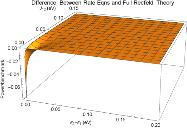
To compare the full Bloch-Redfield treatment to our simplified rate equation model, we need to make additional assumptions about the imaginary parts of the TCL2 generator, which correspond to unitary renormalisation terms that do not feature in the rate equations. Expecting them to be small, we neglect (optical) Lamb shift terms whilst keeping (phonon) reorganisation energies, which we assume to be of the rates given by each bath, i.e. (the precise choice is not important). In Fig. 12 we plot the difference between the power enhancement predicted by the rate equations and full Redfield theory, showing this for both the asymmetric and symmetric models, for the same parameters as in Fig. 3 of the main text. We find that in all cases the secular approximation is fully justified. Figs. 13 shows this difference again this time for the same parameters as in Fig. 4 of the main text. We find that for the asymmetric case, the secular approximation is fully justified whenever the difference between the and the states is sufficiently large, which is the relevant regime for this work. For the symmetric case the two treatments coincide up to numerical inaccuracies of order (not shown).
B.7 Pure Dephasing

We expect phonons to be the dominant source of decoherence and dephasing of our exciton states. Since their effect has already been accounted for based on a microscopic treatment, we here only need to consider small additional contributions, either due to other, unknown physical processes or inadequacies of our microscopic small, which does after all involve some approximations. Therefore, not being able to fall back on microscopically informed dephasing rates, we implement a phenomenological model (similar to the approach taken in, e.g., Ref. 41) to investigate how our results differ when pure dephasing terms defined in the site basis are included. Explicitly, we simply add a Lindblad operator to the Bloch-Redfield treatment, which is given by
| (43) | |||
| (44) |
As discussed above, we expect any additional pure dephasing rate to be much smaller than the level of decoherence that is already accounted for. Taking as an indicative comparative measure, we will consider a dephasing rate that is 5-20% of that.
Fig. 14 shows the maximum relative enhancement of the different models, for the same parameters as in Fig. 3 of the main text. We find that the asymmetric model is very susceptible to pure dephasing, compared to the symmetric one, especially in the very weak coupling to the reaction centre regime. In some cases pure dephasing even brings the otherwise superior asymmetric model below the symmetric one. We believe this is because such pure dephasing, defined with respect to the site basis, effectively corresponds to a non-directional (or infinite temperature) transition , thus degrading the protection against exciton recombination given by the state, which is the main advantage of the asymmetric model over the symmetric one.
References
- [1] Konstantin E Dorfman, Dmitri V Voronine, Shaul Mukamel, and Marlan O Scully, “Photosynthetic reaction center as a quantum heat engine,” Proc. Natl. Acad. Sci. 110, 2746–2751 (2012).
- [2] Tetsuji Tokihiro, Yoshihiro Manabe, and Eiichi Hanamura, “Superradiance of Frenkel excitons in linear systems,” Physical Review B 47, 2019–2030 (1993).
- [3] C. Creatore, M. a. Parker, S. Emmott, and a. W. Chin, “Efficient biologically inspired photocell enhanced by delocalized quantum states,” Physical Review Letters 111, 1–5 (2013).
- [4] N. Killoran, S. F. Huelga, and M. B. Plenio, “Enhancing light-harvesting power with coherent vibrational interactions: A quantum heat engine picture,” The Journal of Chemical Physics 143, 155102 (2015), http://dx.doi.org/10.1063/1.4932307.
- [5] Yiteng Zhang, Sangchul Oh, Fahhad H. Alharbi, Gregory S. Engel, and Sabre Kais, “Delocalized quantum states enhance photocell efficiency,” Phys. Chem. Chem. Phys. 17, 5743–5750 (2015).
- [6] K D B Higgins, B W Lovett, and E M Gauger, “Quantum-enhanced capture of photons using optical ratchet states,” (2015), arXiv:1504.05849v1 .
- [7] Koichiro Mukai, Shuji Abe, and Hitoshi Sumi, “Theory of Rapid Excitation-Energy Transfer from B800 to Optically-Forbidden Exciton States of B850 in the Antenna System LH2 of Photosynthetic Purple Bacteria,” The Journal of Physical Chemistry B 103, 6096–6102 (1999).
- [8] R. E. Fenna and B. W. Matthews, “Chlorophyll arrangement in a bacteriochlorophyll protein from Chlorobium limicola,” Nature 258, 573–577 (1975).
- [9] Jeremy Moix, Jianlan Wu, Pengfei Huo, David Coker, and Jianshu Cao, “Efficient Energy Transfer in Light-Harvesting Systems, III: The Influence of the Eighth Bacteriochlorophyll on the Dynamics and Efficiency in FMO,” The Journal of Physical Chemistry Letters 2, 3045–3052 (2011).
- [10] Julia Adolphs and Thomas Renger, “How proteins trigger excitation energy transfer in the FMO complex of green sulfur bacteria.” Biophysical Journal 91, 2778–97 (2006).
- [11] Akihito Ishizaki and Graham R Fleming, “Theoretical examination of quantum coherence in a photosynthetic system at physiological temperature.” Proceedings of the National Academy of Sciences of the United States of America 106, 17255–17260 (2009).
- [12] Gregory S Engel, Tessa R Calhoun, Elizabeth L Read, Tae-Kyu Ahn, Tomás Mancal, Yuan-Chung Cheng, Robert E Blankenship, and Graham R Fleming, “Evidence for wavelike energy transfer through quantum coherence in photosynthetic systems.” Nature 446, 782–6 (2007).
- [13] Gitt Panitchayangkoon, Dugan Hayes, Kelly a Fransted, Justin R Caram, Elad Harel, Jianzhong Wen, Robert E Blankenship, and Gregory S Engel, “Long-lived quantum coherence in photosynthetic complexes at physiological temperature.” Proceedings of the National Academy of Sciences of the United States of America 107, 12766–70 (2010).
- [14] Yuan-Chung Cheng and Graham R Fleming, “Dynamics of light harvesting in photosynthesis.” Annual review of physical chemistry 60, 241–262 (2009).
- [15] Christoph Kreisbeck and Tobias Kramer, “Long-Lived Electronic Coherence in Dissipative Exciton Dynamics of Light-Harvesting Complexes,” The Journal of Physical Chemistry Letters 3, 2828–2833 (2012).
- [16] Neill Lambert, Yueh-Nan Chen, Yuan-Chung Cheng, Che-Ming Li, Guang-Yin Chen, and Franco Nori, “Quantum biology,” Nature Physics 9, 10–18 (2012).
- [17] Thorsten Ritz, Sanghyun Park, and Klaus Schulten, “Kinetics of Excitation Migration and Trapping in the Photosynthetic Unit of Purple Bacteria,” The Journal of Physical Chemistry B 105, 8259–8267 (2001).
- [18] Alexandra Olaya-Castro, Chiu Fan Lee, Francesca Fassioli Olsen, and Neil F. Johnson, “Efficiency of energy transfer in a light-harvesting system under quantum coherence,” Physical Review B - Condensed Matter and Materials Physics 78, 1–7 (2008), arXiv:0708.1159 .
- [19] a. Shabani, M. Mohseni, H. Rabitz, and S. Lloyd, “Efficient estimation of energy transfer efficiency in light-harvesting complexes,” Physical Review E - Statistical, Nonlinear, and Soft Matter Physics 86, 1–15 (2012), arXiv:1103.3823 .
- [20] Anatoly Yu Smirnov, Lev G Mourokh, Pulak K Ghosh, and Franco Nori, “High-Efficiency Energy Conversion in a Molecular Triad Connected to Conducting Leads,” The Journal of Physical Chemistry C 113, 21218–21224 (2009).
- [21] Mario Einax, Marcel Dierl, and Abraham Nitzan, “Heterojunction Organic Photovoltaic Cells as Molecular Heat Engines: A Simple Model for the Performance Analysis,” The Journal of Physical Chemistry C 115, 21396–21401 (2011), arXiv:1107.0924 .
- [22] Mario Einax, Marcel Dierl, Philip R Schiff, and Abraham Nitzan, “Multiple state representation scheme for organic bulk heterojunction solar cells: A novel analysis perspective,” EPL (Europhysics Letters) 104, 40002 (2013), arXiv:arXiv:1311.6495v2 .
- [23] Shigeru Ajisaka, Bojan Žunkovič, and Yonatan Dubi, “The Molecular Photo-Cell: Quantum Transport and Energy Conversion at Strong Non-Equilibrium,” Scientific Reports 5, 8312 (2015).
- [24] Erik M. Gauger and Joachim Wabnig, “Heat pumping with optically driven excitons,” Phys. Rev. B 82, 073301 (2010).
- [25] See Appendix B.
- [26] H. P. Breuer and F. Petruccione, The Theory of Open Quantum Systems (Clarendon Press, 2007).
- [27] Robert T. Ross, “Some thermodynamics of photochemical systems,” The Journal of Chemical Physics 46, 4590–4593 (1967).
- [28] Richard Stones, Hoda Hossein-Nejad, Rienk van Grondelle, and Alexandra Olaya-Castro, “How a structured vibrational environment controls the performance of a photosystem II reaction centre-based photocell,” , 1–10 (2016), arXiv:1601.05260 .
- [29] Wolfgang Niedenzu, David Gelbwaser-Klimovsky, and Gershon Kurizki, “Performance limits of multilevel and multipartite quantum heat machines,” Phys. Rev. E 92, 042123 (2015).
- [30] Raam Uzdin, Amikam Levy, and Ronnie Kosloff, “Equivalence of Quantum Heat Machines, and Quantum-Thermodynamic Signatures,” Physical Review X 5, 031044 (2015).
- [31] David Gelbwaser-Klimovsky, Wolfgang Niedenzu, and Gershon Kurizki, “Chapter twelve - thermodynamics of quantum systems under dynamical control,” (Academic Press, 2015) pp. 329 – 407.
- [32] Esteban a. Martinez and Juan Pablo Paz, “Dynamics and Thermodynamics of Linear Quantum Open Systems,” Physical Review Letters 110, 130406 (2013), arXiv:1207.4256 .
- [33] Ronnie Kosloff and Amikam Levy, “Quantum Heat Engines and Refrigerators: Continuous Devices,” Annual Review of Physical Chemistry 65, 365–393 (2014).
- [34] Amikam Levy and Ronnie Kosloff, “The local approach to quantum transport may violate the second law of thermodynamics,” EPL (Europhysics Letters) 107, 20004 (2014).
- [35] Rafael Gomez-Bombarelli et al., “Design of efficient molecular organic light-emitting diodes by a high-throughput virtual screening and experimental approach,” Nature Materials , in press (2016).
- [36] R. W. Munn and R. Silbey, “Theory of electronic transport in molecular crystals. II. Zeroth order states incorporating nonlocal linear electron–phonon coupling,” The Journal of Chemical Physics 83, 1843 (1985a).
- [37] R. W. Munn and R. Silbey, “Theory of electronic transport in molecular crystals. III. Diffusion coefficient incorporating nonlocal linear electron–phonon coupling,” The Journal of Chemical Physics 83, 1854 (1985b).
- [38] Yang Zhao, David W. Brown, and Katja Lindenberg, “On the Munn–Silbey approach to nonlocal exciton–phonon coupling,” The Journal of Chemical Physics 100, 2335 (1994).
- [39] Shaul Mukamel and Darius Abramavicius, “Many-Body Approaches for Simulating Coherent Nonlinear Spectroscopies of Electronic and Vibrational Excitons,” Chemical Reviews 104, 2073–2098 (2004).
- [40] Patrick Rebentrost, Masoud Mohseni, and Alan Aspuru-Guzik, “Role of quantum coherence and environmental fluctuations in chromophoric energy transport,” The Journal of Physical Chemistry B 113, 9942–9947 (2009a), pMID: 19603843, http://dx.doi.org/10.1021/jp901724d .
- [41] Patrick Rebentrost, Masoud Mohseni, Ivan Kassal, Seth Lloyd, and Alan Aspuru-Guzik, “Environment-assisted quantum transport,” New Journal of Physics 11, 033003 (2009b).