Low-energy negative muon interaction with matter
Abstract
Using simulated data, obtained with the fluka code, we derive empirical regularities about the propagation and stopping of low-energy negative muons in hydrogen and selected solid materials. The results are intended to help the preliminary stages of the set-up design for experimental studies of muon capture and muonic atom spectroscopy. Provided are approximate expressions for the parameters of the the momentum, spatial and angular distribution of the propagating muons. In comparison with the available data on the stopping power and range of muons (with which they agree in the considered energy range) these results have the advantage to also describe the statistical spread of the muon characteristics of interest.
keywords
Detector modelling and simulations; Charge transport and multiplication in gas; Very low-energy charged particle detectors; Simulation methods and programs1 Introduction
The laser spectroscopy measurement of the hyperfine splitting in the ground state of muonic hydrogen, considered as fundamental test of QED, complementary to the measurement in ordinary hydrogen [1], has been a major experimental challenge for more than two decades [2, 3]. The interest in it grew up significantly when the muonic hydrogen Lamb shift experiment revealed a 9 discrepancy between the proton charge radius values extracted from muonic hydrogen spectroscopy and scattering data [4]. The point was that from the hyperfine splitting of muonic hydrogen one can directly extract the value of the Zemach radius of the proton [5], juxtapose it to the value extracted from ordinary hydrogen spectroscopy [6] and this way test most of the hypotheses put forward to explain the proton size puzzle. The FAMU collaboration [7] is currently preparing an experiment that uses a method based on the study of the diffusion of the hydrogen muonic atoms in appropriate gas target and its response to monochromatic laser radiation of resonance frequency [8, 9]. An alternative experimental approach has been recently suggested in [10].
As discussed in details in [3, 8, 9], the efficiency of this method is determined by the energy dependence in the epithermal range of the rate of muon transfer in collisions of the muonic hydrogen atoms with the atoms of the heavier gas admixture. There are experimental indications that muon transfer to oxygen has the needed characteristics [11], in agreement with the theoretical estimates [12, 13], but the experimental accuracy is far from being sufficient for planning and optimizing the measurement of the hyperfine splitting. Because of this, an experiment uniquely dedicated to the thorough investigation of the collision energy dependence of the rate of muon transfer to various gases was launched as a first stage of the FAMU project. The measurements are to be performed at the pulsed muon source of the RAL-RIKEN facility [14]. Muons of initial momentum in the 50-70 MeV/c range will be stopped in a mixture of hydrogen and various heavier gases at high pressure, and the time distribution of the characteristic X-rays signalling the transfer of the muon to the admixture nuclei will be registered and analyzed using the algorithms of [9].
One of the main challenges in the preparation of the set-up for the above experiment, as well as in other experiments studying muon capture by protons or muonic atom spectroscopy, is the design of the gas target which has to satisfy the following conditions:
- 1.
as much as possible of the incident muons are stopped in gas, i.e. the losses in the front, side and rear walls of the gas container are minimized;
- 2.
as large part as possible of the emitted characteristic X-rays reach the radiation detectors around the gas target that, in principle, cover only a small fraction of the solid angle;
Cond. 1 requires the detailed study of the balance between the stopping power of the target as function of the muon momentum and the pressure (with account of the dependence of the muon flux on the initial momentum), and the losses in the walls that depend on their composition and thickness. Cond. 2 requires the study of the spatial aspects of the muon stopping and the formation of muonic atoms. During the search for the optimal target and detector set-up a large variety of geometrical configurations and materials were considered and investigated with Monte Carlo simulation codes. We noticed that blind iterative simulations are not necessarily the best approach and that it is useful and illuminating to have an analytic formulation allowing to identify the optimal path before proceeding with cross-over simulations. Leaving the detailed description of the selected experimental design for the muon transfer experiment to be reported elsewhere, we present here some characteristics and regularities of the propagation of negative muons in materials, established empirically with the fluka simulation code [15, 16], which we found particularly useful in the preliminary stages of the set-up design and, we believe, are applicable to a broad range of muon physics modelling problems.
We focus our attention on two “elemental” cases: (a) a monochromatic collinear muon beam normally incident on a solid homogeneous layer made out of some of the materials of interest (steel, aluminum, gold, and polystyrene), and (b) a monochromatic collinear muon beam stopped in an unbound domain filled with hydrogen. In case (a), only part of the incident muons cross the layer; they are scattered at angle with final momentum , in general different from the initial momentum . We studied the probability distributions of and as functions of and the layer thickness and derived simple approximate expressions for the mean and root mean squared (r.m.s.) deviation values, as well for the surviving rate . These expressions were verified to provide satisfactory accuracy for MeV/c - the range of interest of initial momenta available at the RAL-RIKEN facility. In case (b) the muons are slowed in collisions with the hydrogen molecules and then stopped and captured in muonic hydrogen atoms. We investigated the spatial distribution of the stopping points and derived simple approximate expressions for the mean value and root mean squared deviation of the cylindrical coordinates and of the stopping points as functions of the initial momentum and the hydrogen gas pressure . In principle, these formulae could be used to model the propagation and stopping of non-monochromatic muon beams in complex geometrical configurations, but undoubtedly such an approach will be much less efficient and accurate that the direct Monte Carlo simulations. The reported results were intended only – and shown to be – a convenient tool for the preliminary estimation of the impact of individual elements during the process of designing complex set-ups for the experimental study of muonic atoms.
2 Propagation of negative muons across solid material layers
In this section we consider the interaction of negative muons with four materials of interest: Aluminum (denoted by A), stainless steel 316LN [17] (S), Gold (G), and Polystyrene (P) using simulated results obtained with the fluka code [15, 16]. In each run monochromatic bunches of muons with initial momentum MeV/c are launched against a layer of material M=A, S, G or P with thickness along the -axis, normal to the layer surface (see Figure 1a).

2.1 Muon survival probability
Denote the number of muons, stopped within the layer, by , . In terms of the latter, the empirical probability distribution for a muon with initial momentum to cross a layer of thickness is . Figure 2 shows “the rate of survival” of a monochromatic muon beam versus the initial momentum , for a set of values of the Aluminum layer thickness .

For momenta below the breakdown thickness-dependent value practically all the muons are stopped in the Al layer; for momenta above practically all muons pass through the layer. The interval of within which rises from % to 80% is as narrow as 1 MeV/c. We defined the breakdown momentum by , evaluated for a set of values of the thickness between 0.01 mm and 8 mm and found out that the following 2-parameter expression fits very well the calculated values:
| (1) |
The values of the parameters and for the material of interest are given in Table 1.
| M | P | A | S | G |
|---|---|---|---|---|
| , MeV/c | 27.3 | 33.3 | 44.0 | 52.7 |
| 0.2842 | 0.2916 | 0.2964 | 0.2997 | |
| , g cm-3 | 1.03 | 2.7 | 7.99 | 19.29 |
It is worth mentioning that the values of the breakdown momentum for the four materials listed above are quite accurately fitted with the single 3-parameter expression
| (2) |
where is the density of the material (in g cm-3, see Table 1), is the thickness (in mm), and MeV/c, , and .
2.2 Momentum and angular composition of the scattered muon beam
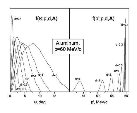
From the simulated data on the final momentum and the scattering angle , obtained with fluka for the muons that cross the layer (see Figure 1) we evaluated the empirical probability densities and of the final momentum and angular distribution of the outgoing muons, as well as the mean values , and the root mean square deviations , of the final momentum and the scattering angle as functions of the initial momentum , the thickness and the material M of the layer. Figure 3 illustrates the shape of the probability density of the momentum and angular distributions of an incident muon beam with 60 MeV/c for aluminum layer thickness in the range mm. Figure 4 shows the dependence of the mean and root mean square values for these distributions on the initial muon momentum .

To make these results helpful for practical use, we fitted the calculated values of , , , and for incident muon momentum MeV/c with the following approximants:
| (3) | |||||
| (4) | |||||
| (5) | |||||
| (6) |
The numerical values of the parameters in these fitting formulae for the materials of interest M=P (polystyrene), A (aluminum), S (stainless steel SS316LN), and G (gold), are given in Tables 2, 3, and 4. The quality of the fit is described with the value of the mean squared deviation
| (7) |
where the summation is over all pairs of values of the parameters ( and in this case) for which the values have been calculated with the fluka code; denotes the value of the fitting function. Each run of fluka used a sample of muons, so that the statistical uncertainty of does not exceed 0.4% and can be neglected with respect to . The numerical uncertainty of the fitting expression coefficients is below , but typing them with more than 4 digits would be in excess of the overall precision.
3 Stopping negative muons in gaseous hydrogen
In this section we use the fluka code to simulate the propagation of negative muons in hydrogen gas target. In each run monochromatic collinear bunches of muons with initial momentum MeV/c are launched in the gas with pressure Atm, the cylindrical coordinates and of the end points of the muon trajectories (where the muons are stopped and supposedly immediately captured in a muonic hydrogen atom, see Figure 1) are registered, and on this basis the empirical density of the spatial distribution of the muon stop points, is evaluated as function of the initial momentum and the hydrogen gas pressure (assuming axial symmetry). Figure 5a is the scatter plot of the set of stopping points for a muon bunch with initial momentum MeV/c, propagating in pure hydrogen at Atm along the -axis. Most of the muons are stopped at about 19 cm from the entry point, with a spread of about cm in both longitudinal and transversal directions. Figure 5b presents the longitudinal density .

As in Section 2, we evaluated the mean values and the r.m.s. deviations of and as functions of the initial momentum and the hydrogen pressure :
| (8) | |||
| (9) |
(and similar for and ). Figure 6 illustrates the dependence of these quantities on the initial muon momentum for hydrogen pressures Atm.

The functional dependence is fitted with expressions of the form:
| (10) |
where the index labels the coefficients of the fit of , , , and , respectively. The numerical values of are given in Table 5.
| M | , % | |||||||
|---|---|---|---|---|---|---|---|---|
| P | ||||||||
| A | ||||||||
| S | ||||||||
| G |
| M | , % | ||||||||
|---|---|---|---|---|---|---|---|---|---|
| P | |||||||||
| A | |||||||||
| S | |||||||||
| G |
4 Verification of the results
Though the results about the propagation of negative muons in selected materials presented above were obtained exclusively by fitting simulated data generated with the widely approved fluka code, they need further verification by comparison with existing experimental and theoretical data.
Most straightforward is the comparison of the mean muon path of Eq. (5) with the CSDA range values of negative muons in hydrogen11 1 See Ref. [18] for definitions, tabulated in [19, 20]. For muon energies above 10 MeV (i.e. MeV/c) we compare with the values of of Ref. [19] that are compatible with [20]. For lower energies the comparison is done with of Ref. [20] since the results of [19] are estimated “not dependable” by the authors themselves. In Table 6 we juxtapose these values of with the values of obtained using Eq. (10), . The good agreement between them confirms the validity of our results for the free path of low-energy muons in gaseous hydrogen. To compare with the available results on the muon range in aluminum, steel, gold and polystyrene, we take into account that the range value is in fact the minimal thickness of a layer of these materials for which 100% of the incident muons with the specified initial energy (or, equivalently, initial momentum , being the muon mass ) are stopped. On the other hand, the breakdown momentum was defined in Subsection 2.1 as the value of the initial momentum for which 50% of the incident muons are stopped in a layer of thickness . Since in the vicinity of the dependence of the fraction of stopped muons is very steep (see Fig. 2b), to a good accuracy we should expect the following relation to hold:
| (11) |
The agreement between the values of and (see Table 6) confirms the validity of the expression of Eq. (1) for the breakdown momentum .
Comparison with the available data on the stopping power of negative muons in Aluminum from Refs. [19, 20] is not straightforward. is defined as
| (12) |
where is the energy of muons of initial energy at the end of a path of length across aluminum with density , evaluated in the CSD approximation. satisfies the relation
| (13) |
for any and , within the CSDA range. What we evaluate instead is the mean energy of a monochromatic bunch of muons with initial energy at the end of a path of length or, to be precise, the energy that corresponds to the mean momentum of a beam with initial momentum . does not satisfy the relation (13): the evolution of the mean energy depends substantially on , as shown on Figure 7(a). The statistical analog of the stopping power of Eq. (12), defined by , also depends on and therefore can be compared with only qualitatively (see Figure 7(b)). For energies of 10 MeV and higher the agreement is reasonable, while for lower energies (the encircled area) is smaller than and approaches zero as . This is due to the fact that in the neighborhood of the breakdown momentum, the final momentum distribution is significantly broadened (see Figure 4) in an asymmetric way so that most of the muons are stopped beyond the CSDA range. This leads in turn to a slower decrease of the mean energy with as compared with , and lower values of in comparison with the stopping power data from Ref. [20].

There also are a few direct measurements of the breakdown momentum in various materials. Ref. [21] reports the experimental value of MeV/c for the breakdown momentum in aluminum plate of thickness 0,81 mg cm-2. The value 6.12 MeV/c obtained with Eq. (1) is in reasonable agreement with experiment. Ref. [22] reports the results of measurements of the energy loss of low-energy muons in thin layers of carbon and gold. Using their data we obtained that muons with initial momentum 1.94 MeV/c (the mean exit momentum for the 20 keV muons launched on the 3.5 g cm-2 carbon backing) cross the 10 m thick gold foil with final momentum MV/c, while Eq. (3) gives 1.79 MeV/c, again in good agreement with experiment.
The tentative formula of Eq. (2) for the breakdown momentum was tested for hydrogen and a few more solid materials, incl. carbon, nickel, copper and zinc, and for low energy muons with momentum up to 75 MeV/c produced results that differ from the what is obtained from Refs. [19] by less than 5%.
Though the angular distribution of muons scattered by various materials has also been the subject of experimental investigations (e.g. in [23]), we did not come across any data that could be directly juxtaposed with values obtained with Eqs. (5) and (6).
| hydrogen | polystyrene | aluminum | steel | gold | |||||||
|---|---|---|---|---|---|---|---|---|---|---|---|
| 1 | |||||||||||
| 10 | |||||||||||
| 14 | |||||||||||
| 20 | |||||||||||
5 Discussion of the results
We start by stressing once again that the results presented here are not aimed at substituting any full scale Monte Carlo simulations but only at helping the early stage design of the set-up for experiments where stopping and capture of low energy muons is studied. Knowing the details of the different types of processes has proven to be useful in restricting the range of the various parameters that are subject to optimization, and significantly enhances the efficiency of the full scale simulations. In what follows we exemplify the usefulness of our approach.
1. Consider the distribution of the muon stopping points along the axis . Figure 5(b) shows the shape of the distribution density under the assumption that all muons enter the gas target with the same momentum . In fact, after crossing the wall of the gas container the incident muon beam is no longer monochromatic and collinear; the distribution density in this case becomes
| (14) |
where is the final momentum distribution density for muons, launched with initial momentum against a layer of M with thickness mm. We approximated it with the normal distribution density
| (15) |
and similar for , performed numerically the integration in (14) and evaluated the FWHH longitudinal spread of the muon stopping area . Figure 8 displays the dependence of on the initial momentum for aluminum plates with thickness 2(1)5 mm and a 1 mm steel plate. The curves have distinct minima for which the muons stopping area is most compact as needed to satisfy Cond. 2, discussed in the Introduction: appropriate positioning the detectors that signal the formation of muonic atoms by registering the characteristic X-rays will maximize their efficiency. The full scale MC search of the optimal initial momentum and detector positions may thus be restricted to a narrower range.

2. The expressions for the mean final momentum approximately satisfy the following scaling relations:
| (16) |
valid for values of above the breakdown momentum by 5-10 MeV/c and higher (see Figure 9). We empirically determined the following values of the material-dependent coefficients : , , , and . The mean values of the angle of deviation , however, are not scaled even approximately. Knowing the angular profile of the muon beam after crossing the entrance window of the gas target is of importance for reducing the losses of muons in the side walls. As long as the angle of deviation in hydrogen gas – of the order of – is much smaller and can be neglected compared to the deviation angle in solid material layers, the preliminary estimate of these losses can be done using Eqs. (5,6).
In a concluding remark we note that, although the detailed study of the propagation of slow muons using the fluka code was restricted here to a few media of specific interest, the apparently wider validity of Eq. (2) makes us believe that the same approach can be efficiently applied to a much broader range of solids and gases, with minimal modifications (if any) in the explicit form of the approximating expressions (3-6) and (10).

Acknowledgements.
The authors are grateful to Dr. G. Battistoni for his help on fluka topics. A.A. and D.B. acknowledge the partial support from the bilateral agreement of the Bulgarian Academy of sciences and the Polish Academy of Sciences.References
- [1] L. Essen, R.W. Donaldson, M.J. Bangham, and E.G. Hope, Frequency of the Hydrogen Maser, Nature 229 (1971) 110.
- [2] D. Bakalov, E. Milotti, C. Rizzo, A. Vacchi, and E. Zavattini, Experimental method to measure the hyperfine splitting of muonic hydrogen . Phys. Lett. A172, (1992) 277.
- [3] A. Adamczak, D. Bakalov, K. Bakalova, E. Polacco, and C. Rizzo, On the use of a mixture gas target in muonic hydrogen atom hyperfine splitting experiments, Hyperfine Interact. 136 (2001) 1.
- [4] R. Pohl, A. Antognini, F. Nez, F. Amaro, and F. Biraben, The size of the proton, Nature 466 (2010) 213.
- [5] A.C. Zemach, Proton Structure and the Hyperfine Shift in Hydrogen, Phys. Rev. 104, 1771 (1956).
- [6] A. Dupays, B. Beswick, C. Rizzo, and D. Bakalov, Proton Zemach radius from measurements of the hyperfine splitting of hydrogen and muonic hydrogen, Phys. Rev. A 68 (2003) 052503.
- [7] https://webint.ts.infn.it/en/research/exp/famu.html
- [8] A. Adamczak, D. Bakalov, L. Stoychev, and A. Vacchi, Hyperfine spectroscopy of muonic hydrogen and the PSI Lamb shift experiment, Nucl. Instrum. Meth. B 281 (2012) 72.
- [9] D. Bakalov, A. Adamczak, M. Stoilov, and A. Vacchi, Theoretical amd computational study of the energy dependence of the muon transfer rate from hydrogen to higher-Z gases, Phys. Lett. A 379 (2015) 151.
- [10] Masaharu Sato, Katsuhiko Ishida, Masahiko Iwasaki, Sohtaro Kanda, Yue Ma, et al.. Laser spectroscopy of the hyperfine splitting energy in the ground state of muonic hydrogen, in proceedings of 20th International Conference on Particles and Nuclei (PANIC 14), 24-29 Aug 2014, Hamburg, Germany, p.460-463. DOI: 10.3204/DESY-PROC-2014-04; ISBN: 9783935702911.
- [11] A. Werthmueller, A. Adamczak, R. Jacot-Guillarmod, et al., Energy dependence of the charge exchange reaction from muonic hydrogen to oxygen, Hyperfine Interact. 116 (1998) 1.
- [12] A. Dupays, B. Lepetit, J. A. Beswick, C. Rizzo and D. Bakalov, Nonzero total-angular-momentum three-body dynamics using hyperspherical elliptic coordinates: Application to muon transfer from muonic hydrogen to atomic oxygen and neon, Phys. Rev. A 69, 062501 (2004).
- [13] Anh-Thu Le, C.D. Lin, Muon transfer from muonic hydrogen to atomic oxygen and nitrogen, Phys. Rev. A 71 (2005) 022507.
- [14] T. Matsuzaki, K. Ishida, K. Nagamine, I. Watanabe, G.H. Eaton, W.G. Willams, Nucl. Instrum. Meth. A 465 (2001) 365-383; http://www.riken.jp/en/research/labs/rnc/ral_office/
- [15] A. Ferrari, P.R. Sala, A. Fasso, and J. Ranft, fluka: a multi-particle transport code, CERN 2005-10 (2005), INFN/TC_05/11, SLAC-R-773.
- [16] T.T. Böhlen, F. Cerutti, M.P.W. Chin, et al., The fluka Code: Developments and Challenges for High Energy and Medical Applications, Nuclear Data Sheets 120, 211-214 (2014).
- [17] For the chemical composition of this grade of stainless steel see, e.g., http://www.matdat.com/; http://www.finetubes.co.uk/uploads/docs/Alloy_316LN.pdf.
- [18] D.E. Groom, N.V. Mokhov, and S. Striganov. Muon stopping power and range, Atomic Data and Nuclear Data Tables 76, 2 (2001).
- [19] http://pdg.lbl.gov/2015/AtomicNuclearProperties/
- [20] http://www.kayelaby.npl.co.uk/
- [21] W. Wilhelm, H. Daniel, and F.J. Hartmann, Measurement of the correction to the stopping power of Al for muons. Phys. Lett B98, 33 (1981).
- [22] P. Wojciechowski, P. Baumann, H. Daniel, et al, Measurement of the stopping power for and at energies between 3 keV and 100 keV, Hyperfine Interact. 82, 127 (1993).
- [23] D. Attwood, P. Bell, S. Bull, et al., The scattering of muons in low Z materials arXiv:hep-ex/0512005(2005).