Decay $B\to K^{\ast}(\to K\pi)\ell^{+}\ell^{-}$ in covariant quark model

The rare flavour changing neutral current (FCNC) decays are forbidden in the Standard Model (SM) at the tree level. They proceed only via loops in the perturbation theory. For this reason, these decays are sensitive to possible effects of new physics beyond the SM. New heavy particles can contribute to the branching fractions and the angular decay distributions.

It is generally believed that the decay mode $B\to K^{\ast}(\to K\pi)\mu^{+}\mu^{-}$ is one of the best modes to search for new physics beyond the SM. The angular distribution makes possible an independent measurement of several observables as a function of the dilepton invariant mass. A large number of observables obtained in this manner allows for unique tests of the SM contributions (see the recent experimental review [1]). A deviation of $3.3\,\sigma$ is seen in e.g. $R(D^{\ast})\equiv\mathcal{B}(B^{-}\to D^{\ast}\tau^{-}\bar{\nu}_{\tau})/\mathcal{B}(B^{-}\to D^{\ast}\ell^{-}\bar{\nu}_{\ell})$ with $R(D^{\ast})|_{\rm expt}=0.321\pm 0.021$ [2] and $R(D^{\ast})|_{\rm SM}=0.252\pm 0.003$ [3, 4, 5, 6]. An analogous result questioning the lepton flavour universality exists also for $B\to K$ decays by Belle [7].

The results of a measurement of form-factor independent angular observables in the decay $B^{0}\rightarrow K^{\ast\,0}(892)\mu^{+}\mu^{-}$ were presented in [8]. The analysis is based on a data sample corresponding to an integrated luminosity of $1.0$ fb^-1, collected by the LHCb experiment in $p\bar{p}$ collisions at a center-of-mass energy of 7 TeV. Four observables are measured in six bins of the dimuon invariant mass squared, $q^{2}$, in the range $0.1<q^{2}<19.0$ GeV². Agreement with the SM predictions is found for 23 of the 24 measurements. A local discrepancy, corresponding to $3.7$ standard deviations, is observed in one $q^{2}$ bin for one of the observables.

The measurements were followed by a large number of publications, with many different scenarios analyzed [9]-[46]. Several authors discuss an appropriate choice of observables with small model dependence, which would discriminate between SM and new physics. Other authors use various assumptions or models to evaluate form factors or study Wilson coefficients (and related operators) in order to make theoretical predictions and, possibly, argue whether the observed deviations do or do not favor a beyond SM explanation.

Our article is devoted to the study of the $B\to K^{\ast}\ell^{+}\ell^{-}$ decay, first, to evaluate the relevant form factors in the framework of the covariant quark model with infrared confinement, and, second, to demonstrate the equivalence of our helicity-based approach with approaches of other autorhs for what concerns the model independent four-fold angular decay distribution and related results. Form factors are then exploited for evaluation of physical observables. The first paper in this direction has been published in 2002, Ref.  [49]. It was one of the first paper where the full four-fold angular decay distribution has been derived for this process in terms of helicity amplitudes including lepton mass effects. However, our model in that time was suffering from lack the of confinement that restricted the range of applications to the hadrons (mesons and baryons) which satisfy the so-called ”threshold inequality”: the hadron mass should be smaller then the total mass of its constituents, i.e. the sum of the constituent quark masses. In this vein, our model was successfully developed for the study of light hadrons (e.g., pion, kaon, baryon octet, $\Delta$-resonance), heavy-light hadrons (e.g., $D$, $D_{s}$, $B$ and $B_{s}$-mesons, $\Lambda_{Q}$, $\Sigma_{Q}$, $\Xi_{Q}$ and $\Omega_{Q}$-baryons) and double heavy hadrons (e.g, $J/\Psi$, $\Upsilon$ and $B_{c}$-mesons, $\Xi_{QQ}$ and $\Omega_{QQ}$ baryons). To extend our approach to other hadrons we had to introduce extra model parameters or do some approximations, like, e.g., to introduce a cutoff parameter for external hadron momenta to guarantee the fulfilment of the above mentioned ”threshold inequality”. Therefore, at that stage we were unable to apply our approach to the study of rare decays involving $K^{\ast}$ mesons. The numerical results for the physical observables were presented in [49] only for decays $B\to K\ell^{+}\ell^{-}$, $B_{c}\to D\ell^{+}\ell^{-}$ and $B_{c}\to D^{\ast}(\to D\pi)\ell^{+}\ell^{-}$.

Our relativistic constituent quark model has been refined in 2009, see Ref. [50], where the confinement of quarks was implemented. It was done, first, by introducing the scale integration in the space of $\alpha$-parameters, and, second, by cutting this scale integration on the upper limit which corresponds to an infrared cutoff. In this manner one removes all possible thresholds present in the initial quark diagram. The cutoff parameter is taken to be the same for all physical processes. Other model parameters were adjusted by fitting the calculated quantities of the basic physical processes to available experimental data. As an application, the electromagnetic form factors of the pion and the transition form factors of the omega and eta Dalitz decays have been calculated.

New values for the parameters of the covariant constituent quark model with built–in infrared confinement have been determined in [51] by a fit to the leptonic decay constants and a number of electromagnetic decays. Then the form factors of the $B(B_{s})\to P(V)$ transitions were evaluated in the full kinematical region of momentum transfer squared in a parameter free way.

The model was than applied to a wide range of nonleptonic and semileptonic meson decays, e.g. [52, 53] and it was extended also to the baryon sector [54, 55, 56, 57, 58]. Different observables related to (nucleons and) heavy $\Lambda$ baryons were calculated in [54, 55, 56, 58]. Furthermore, the consequences of treating the X(3872) meson as a tetraquark bound state were explored in Refs. [59, 60]. Some of the above research was collected in the review [61].

Our paper is organized as follows. In Sec. II we review salient features of the covariant quark model. In Sec. III we present the calculated form factors in the full kinematical momentum transfer region. In Sec. IV we discuss the effective Hamiltonian, matrix elements, invariant and helicity form factors. Sec. V is devoted to the four-fold angular decay distribution in the cascade decay $B\to K^{\ast}(\to K\pi)\bar{\ell}\ell$ and, in particular, to the relation of our helicity formalism with an approach based on the transversality amplitudes which is widely used by both experimentalists and theorists. In Sec. VI we present our numerical results on the branching fractions, forward-backward asymmetry, longitudinal polarization and a set of the so-called “clean” observables $P_{i}$ which depend on the hadron uncertainties (form factors) in a minimal way. Finally, in Sec. VII we summarize our results.

The covariant confined quark model developed in [62, 63, 49, 50] has been applied to a large number of elementary particle processes. This model can be viewed as an effective quantum field approach to hadronic interactions based on an interaction Lagrangian of hadrons interacting with their constituent quarks. The coupling strength is determined by the compositeness condition $Z_{H}=0$ where $Z_{H}$ is the wave function renormalization constant of the hadron. The hadron field renormalization constant $Z_{H}$ characterizes the overlap between the bare hadron field and the bound state formed from the constituents. Once this constant is set to zero, the dynamics of hadron interactions is fully described by constituent quarks in quark loop diagrams with local constituent quark propagators. Matrix elements are generated by a set of quark loop diagrams according to the $1/N_{c}$ expansion. The ultraviolet divergences of the quark loops are regularized by including vertex functions for the hadron-quark vertices which, in addition, describe finite size effects due to the non-pointlike structure of hadrons. Quark confinement was implemented into the model [50] by introducing an infrared cutoff on the upper limit of the scale integration to avoid the appearance of singularities in any matrix element. The infrared cutoff parameter $\lambda$ is taken to have a common value for all processes. The covariant confined quark model contains only a few model parameters: the light and heavy constituent quark masses, the size parameters that describe the size of the distribution of the constituent quarks inside the hadron and the infrared cutoff parameter $\lambda$. They are determined by a fit to available experimental data.

Herein our primary subject is the matrix element which is described by the Feynman diagram shown in Fig. 2. It can be expressed via dimensionless form factors:

Here, $P=p_{1}+p_{2}$, $q=p_{1}-p_{2}$, $\epsilon_{2}^{\dagger}\cdot p_{2}=0$, $p_{i}^{2}=m_{i}^{2}$. Since there are three sorts of quarks involved in these processes, we introduce the notation with two subscripts $w_{ij}=m_{q_{j}}/(m_{q_{i}}+m_{q_{j}})$ $(i,j=1,2,3)$ so that $w_{ij}+w_{ji}=1$. The form factors defined in Eq. (20) satisfy the physical requirement $a_{0}(0)=a_{+}(0)$, which ensures that no kinematic singularity appears in the matrix element at $q^{2}=0$ GeV.

We will use the latest fit done in Ref. [70]. The fitted values of the constituent quark masses $m_{q}$, the infrared cutoff $\lambda$, and the size parameters $\Lambda_{H}$ are given by Eq. (21) and Table 1.

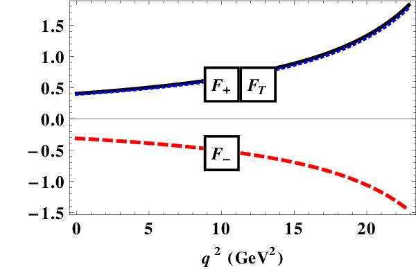
Our form factors are represented as three-fold integrals which are calculated by using NAG routines. They are shown in Figs. 3, 4 and 5. The results of our numerical calculations are well approximated by the parametrization

The values of $F(0)$, $a$, and $b$ are listed in Table 2. One can compare the obtained values of form factors at maximum recoil $q^{2}=0$ with those obtained in other approaches, see, for example, Table IV in [39] and references therein.

The rare exclusive decays are described by the effective Hamiltonian obtained from the SM-diagrams using the operator product expansion and renormalization group techniques. It allows one to separate the short-distance contributions and isolate them in the Wilson coefficients which can be studied systematically within perturbative QCD. The long-distance contributions are contained in the matrix elements of local operators. Contrary to the short-distance contributions the calculation of such matrix elements requires nonperturbative methods and is therefore model dependent.

The rare decay $b\to s(d)\ell^{+}\ell^{-}$ can be described in terms of the effective Hamiltonian [71]:

where $C_{i}(\mu)$ and $\mathcal{O}_{i}(\mu)$ are the Wilson coefficients and local operators, respectively. $\lambda_{t}\equiv|V_{ts}^{\ast}V_{tb}|$ is the product of CKM matrix elements. The standard set [71] of local operators for $b\to sl^{+}l^{-}$ transition is written as

where ${\bf G}_{\mu\nu}$ and $F_{\mu\nu}$ are the gluon and photon field strengths, respectively; ${\bf T}_{a_{1}a_{2}}$ are the generators of the $SU(3)$ color group; $a_{1}$ and $a_{2}$ denote color indices (they are omitted in the color-singlet currents). The chirality projection operators are $P_{L,R}=(1\mp\gamma_{5})/2$ and $\mu$ is a renormalization scale. $\mathcal{O}_{1,2}$ are current-current operators, $\mathcal{O}_{3-6}$ are QCD penguin operators, $\mathcal{O}_{7,8}$ are ”magnetic penguin” operators, and $\mathcal{O}_{9,10}$ are semileptonic electroweak penguin operators.

By using the effective Hamiltonian defined by Eq. (23) one can write the matrix element of the exclusive transition $B\to K^{\ast}\ell^{+}\ell^{-}$ as

where $C_{7}^{\rm eff}=C_{7}-C_{5}/3-C_{6}$. One has to note that matrix element in Eq.(30) contains both a free quark decay amplitude coming from the operators $\mathcal{O}_{7}$, $\mathcal{O}_{9}$ and $\mathcal{O}_{10}$ (gluon magnetic penquin $\mathcal{O}_{8}$ does not contribute) and, in addition, certain long-distance effects from the matrix elements of four-quark operators $\mathcal{O}_{i}\,\,(i=1,\ldots,6)$ which usually are absorbed into a redefinition of the short-distance Wilson-coefficients. The Wilson coefficient $C_{9}^{\rm eff}$ effectively takes into account, first, the contributions from the four-quark operators $\mathcal{O}_{i}$ ($i=1,...,6$) and, second, the nonperturbative effects coming from the $c\bar{c}$-resonance contributions which are as usual parametrized by the Breit-Wigner ansatz [72]:

where $C_{0}\equiv 3C_{1}+C_{2}+3C_{3}+C_{4}+3C_{5}+C_{6}$. Here the charm-loop function is written as

where $\hat{m}_{c}=\bar{m}_{c}/m_{B}$, $s=q^{2}/m_{B}^{2}$ and $\kappa=1/C_{0}$. In what follows we drop the charm resonance contributions by putting $\kappa=0$. We denote the QCD quark masses by the bar symbol to distinguish them from the constituent quark masses used in the model, see Eq. (8). We will use the value of $\mu=\bar{m}_{b\,\rm pole}$ for the renormalization scale. The numerical values for the model-independent input parameters and the corresponding values of the Wilson coefficients are given in Table 4. Besides the charm-loop perturbative contribution, two loop contributions have been calculated in [47]. A global analysis of $b\to s\ell\ell$ anomalies has been performed in Ref. [48] with the NNLL corrections included. It was shown that they amount up to 15$\%$. The discussion of the non-local $c\bar{c}$ contributions maybe also found in Ref. [43].

We specify our choice of the momenta for the reaction $B(p_{1})\to H_{\rm out}(p_{2})+\ell^{+}(k_{1})+\ell^{-}(k_{2})$ as $p_{1}=p_{2}+k_{1}+k_{2}$ with $p_{1}^{2}=m_{1}^{2}$, $p_{2}^{2}=m_{2}^{2}$ and $k_{1}^{2}=k_{2}^{2}=m_{\ell}^{2}$ where $k_{1}$ and $k_{2}$ are the $l^{+}$ and $l^{-}$ momenta, and $m_{1}$, $m_{2}$, $m_{\ell}$ are the masses of the initial $B$ meson, final meson $H_{\rm out}=K,K^{\ast}$ and lepton, respectively.

The matrix element in Eq (30) can now be written

where the quantities $T_{i}^{\mu}$ are expressed through the form factors and the Wilson coefficients in the following manner:

Let us consider the decay distribution differential in the momentum transfer squared $q^{2}$ and in the polar angle. The latter is defined as the angle between $\vec{q}=\vec{p}_{1}-\vec{p}_{2}$ and $\vec{k}_{1}$ ($\ell^{+}\ell^{-}$ rest frame) as shown in Fig. 6. By using the notation from Ref. [49] and correcting some obvious typos, one has

References

• [1] C. Langenbruch [LHCb Collaboration], “Latest results on rare decays from LHCb,” arXiv:1505.04160 [hep-ex].
• [2] A. Crivellin, J. Heeck and P. Stoffer, arXiv:1507.07567 [hep-ph].
• [3] J. Lees et al. (BABAR Collaboration), Phys. Rev. Lett. 109, 101802 (2012). arXiv:1205.5442 [hep-ex].
• [4] M. Tanaka and R. Watanabe, Phys. Rev. D 82, 034027 (2010) [arXiv:1005.4306 [hep-ph]].
• [5] S. Fajfer, J. F. Kamenik, and I. Nisandzic, Phys. Rev. D 85, 094025 (2012). arXiv:1203.2654 [hep-ph].
• [6] J. F. Kamenik and F. Mescia, Phys. Rev. D 78, 014003 (2008). arXiv:0802.3790 [hep-ph].
• [7] R. Aaij et al. [LHCb Collaboration], Phys. Rev. Lett. 113, 151601 (2014) [arXiv:1406.6482 [hep-ex]].
• [8] R. Aaij et al. [LHCb Collaboration], Phys. Rev. Lett. 111, 191801 (2013) [arXiv:1308.1707 [hep-ex]].
• [9] S. Descotes-Genon, J. Matias and J. Virto, Phys. Rev. D 88, 074002 (2013) [arXiv:1307.5683 [hep-ph]].
• [10] S. Descotes-Genon, T. Hurth, J. Matias and J. Virto, JHEP 1305, 137 (2013) [arXiv:1303.5794 [hep-ph]].
• [11] T. Hurth and F. Mahmoudi, JHEP 1404, 097 (2014) [arXiv:1312.5267 [hep-ph]].
• [12] C. Bobeth, G. Hiller and D. van Dyk, JHEP 1007, 098 (2010) [arXiv:1006.5013 [hep-ph]].
• [13] C. Bobeth, G. Hiller and D. van Dyk, Phys. Rev. D 87, no. 3, 034016 (2013) [arXiv:1212.2321 [hep-ph]].
• [14] G. Hiller and R. Zwicky, JHEP 1403, 042 (2014) [arXiv:1312.1923 [hep-ph]].
• [15] J. Gratrex, M. Hopfer and R. Zwicky, arXiv:1506.03970 [hep-ph].
• [16] D. Das, G. Hiller, M. Jung and A. Shires, JHEP 1409, 109 (2014) [arXiv:1406.6681 [hep-ph]].
• [17] L. Hofer and J. Matias, arXiv:1502.00920 [hep-ph].
• [18] S. Descotes-Genon and J. Virto, JHEP 1504, 045 (2015) [arXiv:1502.05509 [hep-ph]].
• [19] S. Descotes-Genon, J. Matias, M. Ramon and J. Virto, JHEP 1301, 048 (2013) [arXiv:1207.2753 [hep-ph]].
• [20] W. Altmannshofer and D. M. Straub, Eur. Phys. J. C 73, 2646 (2013) [arXiv:1308.1501 [hep-ph]].
• [21] R. Mandal, R. Sinha, and D. Das, Phys. Rev. D 90, 096006 (2014) [arXiv:1409.3088 [hep-ph]].
• [22] J.G. Körner, G.A. Schuler: Z. Phys. C 38 (1988) 511 [Erratum-ibid. C 41 (1989) 690]; Z. Phys. C 46 (1990) 93.
• [23] D. Melikhov, N. Nikitin and S. Simula, Phys. Lett. B 442, 381 (1998) [hep-ph/9807464].
• [24] F. Kruger, L. M. Sehgal, N. Sinha and R. Sinha, Phys. Rev. D 61, 114028 (2000) [ Erratum-ibid. D 63, 019901 (2001)] [hep-ph/9907386].
• [25] C. S. Kim, Y. G. Kim, C. D. Lu and T. Morozumi, Phys. Rev. D 62, 034013 (2000) [hep-ph/0001151].
• [26] F. Kruger and J. Matias, Phys. Rev. D 71, 094009 (2005) [hep-ph/0502060].
• [27] F. Kruger and L. M. Sehgal, Phys. Lett. B 380, 199 (1996) [hep-ph/9603237].
• [28] J. Matias, F. Mescia, M. Ramon and J. Virto, JHEP 1204, 104 (2012) [arXiv:1202.4266 [hep-ph]].
• [29] U. Egede, T. Hurth, J. Matias, M. Ramon and W. Reece, JHEP 1010, 056 (2010) [arXiv:1005.0571 [hep-ph]].
• [30] M. Beneke, T. Feldmann and D. Seidel, Nucl. Phys. B 612, 25 (2001) [hep-ph/0106067].
• [31] H. H. Asatryan, H. M. Asatrian, C. Greub and M. Walker, Phys. Rev. D 65, 074004 (2002) [hep-ph/0109140].
• [32] C. H. Chen and C. Q. Geng, Phys. Rev. D 63, 114025 (2001) [hep-ph/0103133].
• [33] C. H. Chen and C. Q. Geng, Nucl. Phys. B 636, 338 (2002) [hep-ph/0203003].
• [34] A. Ali and A. S. Safir, Eur. Phys. J. C 25, 583 (2002) [hep-ph/0205254].
• [35] T. Feldmann and J. Matias, JHEP 0301, 074 (2003) [hep-ph/0212158].
• [36] P. Ball and R. Zwicky, Phys. Rev. D 71, 014029 (2005) [hep-ph/0412079].
• [37] A. Khodjamirian, T. Mannel and N. Offen, Phys. Rev. D 75, 054013 (2007) [hep-ph/0611193].
• [38] M. A. Ivanov, Y. L. Kalinovsky, P. Maris and C. D. Roberts, Phys. Rev. C 57, 1991 (1998) [nucl-th/9711023].
• [39] M. A. Ivanov, J. G. Körner, S. G. Kovalenko and C. D. Roberts, Phys. Rev. D 76, 034018 (2007) [nucl-th/0703094].
• [40] D. Ebert, R. N. Faustov and V. O. Galkin, Phys. Rev. D 82, 034032 (2010) [arXiv:1006.4231 [hep-ph]].
• [41] A. Khodjamirian, T. Mannel, A. A. Pivovarov and Y.-M. Wang, JHEP 1009, 089 (2010) [arXiv:1006.4945 [hep-ph]].
• [42] A. K. Alok, A. Dighe, D. Ghosh, D. London, J. Matias, M. Nagashima and A. Szynkman, JHEP 1002, 053 (2010) doi:10.1007/JHEP02(2010)053 [arXiv:0912.1382 [hep-ph]].
• [43] M. Beylich, G. Buchalla and T. Feldmann, Eur. Phys. J. C 71 (2011) 1635 doi:10.1140/epjc/s10052-011-1635-0 [arXiv:1101.5118 [hep-ph]].
• [44] X. W. Kang, B. Kubis, C. Hanhart and U. G. Meißner, Phys. Rev. D 89, 053015 (2014) doi:10.1103/PhysRevD.89.053015 [arXiv:1312.1193 [hep-ph]].
• [45] J. Lyon and R. Zwicky, arXiv:1406.0566 [hep-ph].
• [46] A. Bharucha, D. M. Straub and R. Zwicky, arXiv:1503.05534 [hep-ph].
• [47] C. Greub, V. Pilipp and C. Schupbach, JHEP 0812, 040 (2008) [arXiv:0810.4077 [hep-ph]].
• [48] S. Descotes-Genon, L. Hofer, J. Matias and J. Virto, arXiv:1510.04239 [hep-ph].
• [49] A. Faessler, T. Gutsche, M. A. Ivanov, J. G. Körner and V. E. Lyubovitskij,
Eur. Phys. J. direct C 4, 18 (2002) [hep-ph/0205287].
• [50] T. Branz, A. Faessler, T. Gutsche, M. A. Ivanov, J. G. Körner, V. E. Lyubovitskij, Phys. Rev. D 81, 034010 (2010). [arXiv:0912.3710 [hep-ph]].
• [51] M. A. Ivanov, J. G. Körner, S. G. Kovalenko, P. Santorelli and G. G. Saidullaeva, Phys. Rev. D 85, 034004 (2012) [arXiv:1112.3536 [hep-ph]].
• [52] S. Dubnička, A. Z. Dubničková, M. A. Ivanov and A. Liptaj, Phys. Rev. D 87, 074201 (2013) [arXiv:1301.0738 [hep-ph]].
• [53] A. Issadykov, M. A. Ivanov and S. K. Sakhiyev, Phys. Rev. D 91, no. 7, 074007 (2015) [arXiv:1502.05280 [hep-ph]].
• [54] T. Gutsche, M. A. Ivanov, J. G. Körner, V. E. Lyubovitskij and P. Santorelli, Phys. Rev. D 86, 074013 (2012) [arXiv:1207.7052 [hep-ph]].
• [55] T. Gutsche, M. A. Ivanov, J. G. Körner, V. E. Lyubovitskij and P. Santorelli, Phys. Rev. D 87, 074031 (2013) [arXiv:1301.3737 [hep-ph]].
• [56] T. Gutsche, M. A. Ivanov, J. G. Körner, V. E. Lyubovitskij and P. Santorelli, Phys. Rev. D 88, no. 11, 114018 (2013) [arXiv:1309.7879 [hep-ph]].
• [57] T. Gutsche, M. A. Ivanov, J. G. Körner, V. E. Lyubovitskij and P. Santorelli, Phys. Rev. D 90, no. 11, 114033 (2014) [arXiv:1410.6043 [hep-ph]].
• [58] T. Gutsche, M. A. Ivanov, J. G. Körner, V. E. Lyubovitskij, P. Santorelli and N. Habyl, Phys. Rev. D 91, no. 7, 074001 (2015) [arXiv:1502.04864 [hep-ph]].
• [59] S. Dubnička, A. Z. Dubničková, M. A. Ivanov and J. G. Körner, Phys. Rev. D 81, 114007 (2010) [arXiv:1004.1291 [hep-ph]].
• [60] S. Dubnička, A. Z. Dubničková, M. A. Ivanov, J. G. Koerner, P. Santorelli, G. G. Saidullaeva, Phys. Rev. D84, 014006 (2011). [arXiv:1104.3974 [hep-ph]].
• [61] M. Dineykhan, M. A. Ivanov and G. G. Saidullaeva, Phys. Part. Nucl. 43, 749 (2012).
• [62] G. V. Efimov and M. A. Ivanov, Int. J. Mod. Phys. A 4, 2031 (1989).
• [63] G. V. Efimov and M. A. Ivanov, The Quark Confinement Model of Hadrons, (CRC Press, Boca Raton, 1993).
• [64] S. Weinberg, Phys. Rev. 130, 776 (1963).
• [65] A. Salam, Nuovo Cimento 25, 224 (1962).
• [66] K. Hayashi, M. Hirayama, T. Muta, N. Seto, and T. Shirafuji, Fortsch. Phys. 15, 625 (1967).
• [67] J. A. M. Vermaseren, Nucl. Phys. Proc. Suppl. 183, 19 (2008) [arXiv:0806.4080 [hep-ph]]; arXiv:math-ph/0010025.
• [68] D. Ebert, T. Feldmann and H. Reinhardt, Phys. Lett. B 388, 154 (1996) [arXiv:hep-ph/9608223].
• [69] M. A. Bedolla, J. J. Cobos-Martínez and A. Bashir, Phys. Rev. D 92, no. 5, 054031 (2015).
• [70] G. Ganbold, T. Gutsche, M. A. Ivanov and V. E. Lyubovitskij, J. Phys. G 42, no. 7, 075002 (2015) [arXiv:1410.3741 [hep-ph]].
• [71] G. Buchalla, A. J. Buras and M. E. Lautenbacher, Rev. Mod. Phys. 68, 1125 (1996) [hep-ph/9512380].
• [72] A. Ali, T. Mannel, T. Morozumi: Phys. Lett. B 273 505 (1991).
• [73] K. A. Olive et al. [Particle Data Group Collaboration], Chin. Phys. C 38, 090001 (2014).
• [74] R. Aaij et al. [LHCb Collaboration], JHEP 1406, 133 (2014) [arXiv:1403.8044 [hep-ex]].
• [75] L. Pescatore [LHCb Collaboration], “Rare decays at the LHCb experiment,” arXiv:1410.2411 [hep-ex].
• [76] A. Ali, E. Lunghi, C. Greub and G. Hiller, Phys. Rev. D 66 (2002) 034002 [hep-ph/0112300].
• [77] A. Ali, P. Ball, L. T. Handoko and G. Hiller, Phys. Rev. D 61 (2000) 074024 [hep-ph/9910221].
• [78] D. Melikhov, N. Nikitin and S. Simula, Phys. Rev. D 57 (1998) 6814 [hep-ph/9711362].
• [79] C. Q. Geng and C. P. Kao, Phys. Rev. D 54 (1996) 5636 [hep-ph/9608466].
• [80] M. A. Ivanov, Y. L. Kalinovsky and C. D. Roberts, Phys. Rev. D 60 (1999) 034018 [nucl-th/9812063].
• [81] Belle Collaboration, Phys. Rev. Lett. 103, 171801 (2009) [arXiv:0904.0770 [hep-ex]].
• [82] LHCb Collaboration, Phys. Rev. Lett. 108, 181806 (2012), [LHCb-CONF-2012-008 and arXiv:1112.3515 [hep-ex]].
• [83] CDF Collaboration, Phys. Rev. Lett. 108, 081807 (2012) [arXiv:1108.0695 [hep-ex]].