2MTF V. Cosmography, , and the residual bulk flow
Abstract
Using the Tully-Fisher relation, we derive peculiar velocities for the 2MASS Tully-Fisher Survey and describe the velocity field of the nearby Universe. We use adaptive kernel smoothing to map the velocity field, and compare it to reconstructions based on the redshift space galaxy distributions of the 2MASS Redshift Survey (2MRS) and the IRAS Point Source Catalog Redshift Survey (PSCz). With a standard minimization fit to the models, we find that the PSCz model provides a better fit to the 2MTF velocity field data than does the 2MRS model, and provides a value of in greater agreement with literature values. However, when we subtract away the monopole deviation in the velocity zeropoint between data and model, the 2MRS model also produces a value of in agreement with literature values. We also calculate the ‘residual bulk flow’: the component of the bulk flow not accounted for by the models. This is km s-1 when performing the standard fit, but drops to km s-1 for both models when the aforementioned monopole offset between data and models is removed. This smaller number is more in line with theoretical expectations, and suggests that the models largely account for the major structures in the nearby Universe responsible for the bulk velocity.
Keywords:
cosmology: distance scale – cosmology: large-scale structure of Universe – galaxies: fundamental parameters – galaxies: distances and redshifts – galaxies: spiral1 Introduction
The velocity field of galaxies exhibits deviations from Hubble flow due to inhomogeneities in the large-scale distribution of matter. By studying the galaxy peculiar velocity field, we can explore the large-scale distribution of matter in the local Universe and so test cosmological models and measure cosmological parameters.
With representing the speed of light and representing a galaxy’s peculiar velocity, we define the ‘peculiar redshift’ as the peculiar velocity in redshift units, given by
| (1) |
where is related to the observed redshift and the redshift due to Hubble flow according to
| (2) |
as given by Harrison (1974). The low redshift approximation of this relation is
| (3) |
where is the Hubble constant and is the galaxy’s comoving distance.
The measurement of peculiar velocities is thus intertwined with the measurement of distances, in that redshift-independent distances are needed in combination with redshifts to extract peculiar velocities. Most of the largest peculiar velocity surveys have made use of one of two redshift-independent distance indicators: the Tully-Fisher relation (TF; Tully & Fisher 1977) and the Fundamental Plane relation (FP; Djorgovski & Davis 1987, Dressler et al. 1987). These scaling relations express the luminosity of a spiral galaxy as a power-law function of its rotational velocity and the radius of an elliptical galaxy as a power law function of its surface brightness and velocity dispersion respectively.
The earliest peculiar velocity surveys using these distance indicators, such as Aaronson et al. (1982) and Lynden-Bell et al. (1988), included no more than a few hundred galaxies. Many of these surveys were concatenated into the Mark III catalog (Willick et al. 1995, Willick et al. 1996). Among the earliest individual TF surveys to include more than galaxies were a set of surveys conducted by Giovanelli, Haynes, and collaborators (e.g., Giovanelli et al. 1994, Giovanelli et al. 1995, Giovanelli et al. 1997a, Haynes et al. 1999a, Haynes et al. 1999b). These surveys were combined, along with additional data, to create the SFI++ survey (Masters et al. 2006; Springob et al. 2007), which included TF data for galaxies.
At the time of its release, SFI++ was the largest peculiar velocity survey compiled. However, both its selection criteria and data sources were quite heterogeneous. The 2MASS Tully-Fisher survey (2MTF) was envisioned as a ‘cleaner’ all-sky TF survey, with more stringent selection criteria, drawn from a more homogeneous dataset, and extending to significantly lower Galactic latitudes. It draws on galaxies selected from the 2MASS Redshift Survey (2MRS, Huchra et al. 2012), and uses photometry from the 2MASS Extended Source Catalogue (Jarrett et al., 2000) and spectroscopy from the Green Bank Telescope (GBT), Parkes radio telescope, Arecibo telescope, and other archival HI catalogs. The archival data overlaps heavily with the archival dataset used for SFI++, and the HI width measurement procedure and peculiar velocity derivation also follows the SFI++ procedure closely. The 2MTF template relation was presented by Masters, Springob, & Huchra (2008), while the first cosmological analysis using the dataset, a measurement of the bulk flow, was presented by Hong et al. (2014).
In this paper, we examine the cosmography of the observed 2MTF velocity field, and compare it to two reconstructions of the predicted peculiar velocity field, which assume that the matter distribution traces the galaxy distribution. The first is the Erdogdu et al. (submitted, updated from Erdoğdu et al. 2006) reconstruction of the aforementioned 2MRS. The second is the Branchini et al. (2001) reconstruction of the IRAS Point Source Catalog Redshift Survey (PSCz, Saunders et al. 2000). In comparing to these reconstructions, we compute the agreement between the observed and predicted velocity fields, the value of the redshift space distortion parameter , and the amplitude and direction of the ‘residual bulk flow’, which represents the component of the bulk flow of the local universe not predicted by models.
The history of such comparisons between observed peculiar velocity fields and predictions made from large all-sky redshift surveys goes back to analyses such as those of Kaiser et al. (1991), Shaya, Tully, & Pierce (1992), Hudson (1994), Davis, Nusser, & Willick (1996), and Hudson et al. (2004). More recently, we have seen the comparisons between SFI++ and 2MRS performed by Davis et al. (2011), between SFI++ and 2M++ (Lavaux & Hudson, 2011) performed by Carrick et al. (2015), and between the 6dF Galaxy Survey (6dFGS) peculiar velocity field (Springob et al., 2014) and both the 2MRS and PSCz reconstructions performed by Magoulas (2012), Magoulas et al. (in prep.), and Springob et al. (2014). These later papers find good overall agreement between the observed and predicted velocity fields, but disagree on whether the predicted fields can explain the amplitude of the bulk flow. 2MTF is well suited to examine this issue because of its all-sky coverage, sampling the sky down to Galactic latitudes of .
The paper is arranged as follows: In Section 2, we describe the 2MTF observational dataset as well as the 2MRS and PSCz model velocity fields. In Section 3, we describe the derivation of peculiar velocities. In Section 4, we describe the cosmography of the 2MTF velocity field, present our comparison of the field to the model velocity fields, and discuss our results. We summarize our results in Section 5.
2 Data
2.1 2MTF TF data
The 2MTF target list was compiled from the set of all 2MRS (Huchra et al., 2012) spirals with total K-band magnitude , CMB frame redshift km s-1, and axis ratio . There are galaxies that meet these criteria, though many of them are quite faint in HI, and observationally expensive to observe with the available single dish radio telescopes. Thus only a fraction of these objects are included in the final 2MTF sample.
We have combined archival data with observations made as part of the Arecibo Fast Legacy ALFA Survey (Giovanelli et al., 2005), and observations made with the Green Bank Telescope (Masters et al., 2014) and Parkes Telescope (Hong et al., 2013). While the new GBT and Parkes observations preferentially targeted late type spirals, the archival data includes all spiral types. The complete 2MTF sample includes 2018 galaxies (note that this is separate from the 888 cluster galaxies used to fit the template TF relation in Masters, Springob, & Huchra 2008). However, as noted in Section 3.2, for the analysis performed in this paper, we exclude large outliers from the TF relation, which reduces the number of objects to 1985.
2.1.1 Photometric Data
All of our photometry is drawn from the 2MRS catalog. 2MRS is an all-sky redshift survey, consisting of redshifts of 2MASS galaxies, extending in magnitude to and Galactic latitude . While the final sample (Huchra et al., 2012) has a limiting K-band magnitude of 11.75, the 2MTF survey began before 2MRS was complete, and so the magnitude limit was set to the somewhat shallower value of 11.25. For the analysis presented in this paper, we use total K-band magnitudes.
While the Masters, Springob, & Huchra (2008) template used I-band and J-band axis ratios, we use 2MASS J/H/K co-added axis ratios (see Jarrett et al. 2000). As explained by Hong et al. (2014), the dispersion between these two definitions of axis ratio is , and we account for this in deriving the scatter of the TF relation, but find no systematic trend between the two definitions towards larger or smaller values.
Internal dust extinction and -correction were done as described by Masters, Springob, & Huchra (2008), and updated in the erratum Masters, Springob, & Huchra (2014). The 2MRS total magnitudes are already corrected for Galactic extinction, so no further correction is necessary.
2.1.2 Spectroscopic Data
The primary source of archival data used here is the Cornell HI archive (Springob et al., 2005), which offers HI spectroscopy for galaxies in the local universe, as observed by single dish radio telescopes. We find 1038 galaxies from this dataset with high quality spectra that match the 2MTF selection criteria. We also include HI data from Theureau et al. (1998), Theureau et al. (2005), Theureau et al. (2007), and Matthewson, Ford, & Buchhorn (1992), as well as the Nancay observations from Table A.1 of Paturel et al. (2003). The raw observed HI widths drawn from these sources were then corrected for inclination, redshift stretch, instrumental effects, turbulence, and smoothing, according to the prescriptions of Springob et al. (2005), which were then updated by Hong et al. (2013).
To supplement the archival data, we made new observations using the Parkes and Green Bank telescopes between 2006 and 2012. These datasets were presented by Hong et al. (2013) and Masters et al. (2014) respectively, but we briefly summarize them here.
The observations were divided up in such a way that Parkes was used to target galaxies in southern declinations (), while the GBT targeted more northern galaxies (), but outside the ALFALFA survey region. (See Figure 1 for the sky distribution of objects.) The GBT observations targeted 1193 galaxies in position switched mode, with the spectrometer set at 9 level sampling with 8192 channels. After smoothing, the velocity resolution was 5.15 km s-1. 727 galaxies were detected, with 483 of them being deemed sufficiently high quality detections to be included in our sample.
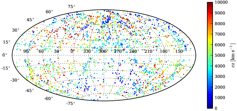
For the Parkes observations, we targeted 305 galaxies which did not already have high quality HI width measurements in the literature. Of these, we obtained width measurements suitable for inclusion in our sample for 152 galaxies. The multibeam correlator produced raw spectra with a velocity resolution of 1.6 km s-1, though Hanning smoothing broadened the resolution to 3.3 km s-1. Each of the GBT and Parkes spectra were analyzed using the IDL routine awv_fit.pro, which is based on the method used for the Cornell HI archive (Springob et al., 2005), which in turn is based on the earlier approach developed by Giovanelli, Haynes, and collaborators (e.g., Giovanelli et al. 1997b). We use the width algorithm, as defined in those papers. It involves fitting a line to either side of the HI line profile, and measuring the width from the points on each line representing of the flux minus rms value. This approach was also adopted for use in the ALFALFA survey.
In addition to the archival, GBT, and Parkes datasets, we also included ALFALFA data from the initial data release (Haynes et al, 2011). The catalog presented in that data release covers roughly of the final survey. However, the ALFALFA team has provided us with additional unpublished data from the survey, current as of October 2013. In total then, we cover of the ALFALFA sky. From this sample, we use 576 galaxy widths, which will be updated once the final release of ALFALFA is available.
As noted above, this gives us a final sample of 1985 galaxies when TF outliers are excluded. The redshift histogram of this sample can be found in Figure 2.

2.2 PSCz model velocity field
The IRAS Point Source Catalog Redshift Survey (PSCz, Saunders et al. 2000) includes 15,500 galaxies, covering of the sky, with most of the missing sky area lying at low Galactic latitudes. Branchini et al. (1999) reconstructs the local density and velocity field from this survey, using a spherical harmonic expansion method proposed by Nusser & Davis (1994). The method assumes a linear mapping between the PSCz spatial distribution of galaxies and the matter distribution, with an input assumed bias parameter . The grid spacing of the model is 2.8 Mpc, extending to a distance of Mpc from the origin in each direction.
We convert the PSCz velocity grid from real space to redshift space, so that we may compare to the redshift space positions of the 2MTF galaxies. Each gridpoint is assigned to its position in redshift space by adding its reconstructed peculiar velocity to its real distance. The reconstructed velocities are then linearly interpolated onto a regularly spaced grid (again with 2.8 Mpc resolution) in redshift space. The problem of triple-valued regions is mitigated in the original Branchini et al. (1999) reconstruction, by the authors collapsing galaxies within clusters, and applying a method devised by Yahil et al. (1991) to determine the locations of galaxies along those lines of sight.
Following the reconstruction of the PSCz velocities onto this redshift space grid, we assign line-of-sight predicted PSCz velocities to each of the galaxies in the 2MTF sample. This is done by interpolating the nearest gridpoints to the position of the galaxy in question. The interpolation is done with inverse distance weighting. This method was also used by Springob et al. (2014) to match 6dFGS peculiar velocities to predictions from models.
2.3 2MRS model velocity field
We also make use of a density/velocity field reconstruction from 2MRS itself. As noted in Section 2.1, the final 2MRS data release (Huchra et al., 2012) includes redshifts for 44,699 galaxies, and covers of the sky (excluding only the Galactic zone of avoidance). Erdoğdu et al. (2006) reconstructed the density/velocity field from an earlier 2MRS data release (Huchra et al., 2005), and this has now been updated to make use of the final dataset (Erdoğdu et al. submitted).
The reconstruction method is described in detail by Erdoğdu et al. (2006). It most closely follows the method used by Fisher et al. (1995), again assuming that the matter distribution follows the galaxy distribution, with an assumed . It involves decomposing the redshift space density field of galaxies into spherical harmonics, and smoothing with a Wiener filter. The reconstruction gives densities and velocities on a grid in supergalactic cartesian coordinates with gridpoints spaced by 8 Mpc and extending to a distance of 200 Mpc from the origin in each direction.
As with PSCz, we convert this grid from real space to redshift space. The resulting redshift space grid in this case has grid spacing of 4 Mpc. Again, as with PSCz, we then use interpolation between gridpoints to assign model velocities to galaxies in the 2MTF sample.
3 Tully-Fisher distances and peculiar velocities
We follow the same basic procedure that was followed for the SFI++ derivation of peculiar velocities by Springob et al. (2007), which relied on the calibration of the TF relation from the template relation of Masters et al. (2006). This in turn followed the procedure used by the SFI and SCI surveys (Giovanelli et al. 1994, Giovanelli et al. 1995, Giovanelli et al. 1997b).
In brief, we use the J-, H-, and K-band TF template relations from Masters, Springob, & Huchra (2008) to derive the peculiar velocities of the individual galaxies in our sample. The Masters, Springob, & Huchra (2008) template sample includes 888 galaxies, while the sample presented in this paper includes 1985 galaxies which does not overlap with the template sample. The template relations found by Masters, Springob, & Huchra (2008) are
| (4) | ||||
where is the corrected HI width in units of km s-1, and , , and are the corrected absolute magnitudes in the three bands.
One difference between the SFI++ approach and the one employed here is that we work with logarithmic distance ratios throughout, rather than converting to linear peculiar velocities. This is done because the distance errors (as well as the individual errors on line width and magnitude) are approximately log-normal. We thus make use of the quantity
| (5) |
where is the difference between the corrected absolute magnitude , calculated using the redshift distance of the galaxy (), and the magnitude derived from the TF template relation. is the distance to the galaxy derived from the Tully-Fisher relation, but not corrected for Malmquist/selection bias. We then refer to as the logarithmic distance ratio (uncorrected for Malmquist bias). In Section 3.2, we discuss the Malmquist bias correction, at which point this quantity is replaced by , the logarithmic distance ratio (corrected for Malmquist bias).
As noted by Hong et al. (2014), the fact that Masters, Springob, & Huchra (2008) uses a different set of axial ratios means that we must derive new measurements of the intrinsic scatter in the TF relation. Hong et al. (2014) does this, and arrives at the relations
| (6) | ||||
for the scatter in the TF relation in magnitude units. To convert these to logarithmic distance units, one must divide the values by 5.
3.1 Galaxy groups
Crook et al. (2007) describes a galaxy group catalog for 2MRS, derived using a ‘friends-of-friends’ algorithm. 55 of these groups include more than one member in our sample. To eliminate the effects of motions within galaxy groups, we thus fix the redshift used when calculating the logarithmic distance ratio in Equation 5 to the group redshift for all of our group galaxies. However, the magnitude offset is still calculated separately for each galaxy.
3.2 Selection bias
‘Malmquist bias’ is the term used to describe biases originating from the interaction between the spatial distribution of objects and the selection effects (Malmquist, 1924). It results from the coupling between the random distance errors and the apparent density distribution along the line of sight. There are two types of distance errors to consider. The first is ‘inhomogeneous Malmquist bias’, which arises from local density variations due to large-scale structure along the line of sight. This bias is most pronounced when measuring galaxy distances in real space. This is because the large distance errors scatter the measured galaxy distances away from overdense regions, creating artificially inflated measurements of infall onto large structures. By contrast, when the measurement is done in redshift space, the much smaller redshift errors mean that this effect tends to be negligible (see e.g.,Strauss & Willick 1995).
For the 2MTF sample, we are measuring galaxy distances and peculiar velocities in redshift space rather than real space. In this case, inhomogeneous Malmquist bias is negligible, and the form of Malmquist bias that we must deal with is of the second type, known as homogeneous Malmquist bias, which affects all galaxies independently of their position on the sky. It is a consequence of both (1) the volume effect, which means that more volume is covered within a given solid angle at larger distances than at smaller distances, and (2) the selection effects, which cause galaxies of different luminosities, radii, velocity dispersions etc., to be observed with diminishing completeness with increased distance. We note, however, that different authors use somewhat different terminology, and the latter effect described above is often simply described as ‘selection bias’.
The approach one takes in correcting for this bias depends in part on the selection effects of the survey. In our case, we used homogeneous criteria in determining which galaxies to observe. However, many of the galaxies that met our selection criteria yielded nondetections, marginal detections, or there was some other problem with the spectrum that precluded the galaxy’s inclusion in our sample. Our final sample, then, lacks the same homogeneity as the original target sample, and our selection bias correction procedure must account for this.
We adopt the following procedure:
1) Using the stepwise maximum likelihood method (Efstathiou, Ellis, & Peterson, 1988), we derive the K-band luminosity function , as a function of K-band absolute magnitude , for all galaxies in 2MRS that meet our K-band apparent magnitude, Galactic latitude, morphological, and axis ratio criteria. For this purpose, we include galaxies beyond the 10,000 km s-1redshift limit, to simplify the implementation of the luminosity function derivation. The resulting luminosity function of this sample is found in Figure 3. We fit a Schechter function (Press & Schechter, 1974) to this distribution, and find parameters and . The final parameter of the Schechter function is the normalization. The stepwise maximum likelihood method cannot derive this parameter, but it is not needed for our method in any case. This luminosity function has a steeper slope than the 2MASS K-band luminosity function dervied by Kochanek et al. (2001), who find . Our morphological selection criteria presumably contribute to this difference, though Jones et al. (2006) notes that there is some disagreement between the Kochanek et al. (2001) luminosity function and others.

2) We define the ‘completeness’ as the fraction of the target sample that is included in our final catalog for a given apparent magnitude bin. We divide up the sky between two regions: one covering all declinations north of , and the other covering all declinations south of . The boundary is the declination at which the sample transitions from GBT to Parkes observations. After experimenting with further subdivisions of the sky, we conclude that the completeness as a function of apparent magnitude remains constant within each region, and assume that that holds in the analysis that follows. We compute this completeness function separately for the two sky regions, by taking the ratio of observed galaxies to galaxies in the target sample for K-band apparent magnitude bins of width 0.25 mag.
3) For each of the galaxies in the sample, we compute the uncorrected logarithmic distance ratio () probability distribution, assuming a Gaussian distribution, with an uncorrected scatter of . For each logarithmic distance ratio value () within of the nominal value of , we weight the probability by , where is the completeness (from Step 2) integrated across the K-band luminosity function (from Step 1), evaluated at the in question. Using the luminosity function in this manner involves converting it into apparent magnitudes, using the relevant distance modulus.
4) Finally, we fit a Gaussian to the re-weighted probability distribution. This gives us the corrected logarithmic distance ratio (), and its error (). We then cut from the sample any galaxies deemed outliers, defined as those for which the deviation from cannot be accounted for by the quadrature sum of a 300 km s-1scatter in peculiar velocities plus deviation from the TF relation. 43 galaxies are eliminated by this criterion, leaving us with a total sample of 1985 galaxies.
The histograms can be found in Hong et al. (2014). As noted in that paper, the mean TF distance error translates to in all three wavebands.
4 Results and discussion
4.1 Velocity field cosmography
Because of the significant distance errors obtained for each individual galaxy, we use adaptive kernel smoothing to get a cosmographic view of the velocity field. We set up a 3D redshift space grid in supergalactic cartesian coordinates, with all gridpoints spaced 4Mpc apart. At each gridpoint, we compute adaptively smoothed values of for both the PSCz reconstructed velocity field, and the observed 2MTF field. This is done following a procedure outlined in Springob et al. (2014), that draws on methods used by Silverman (1986) and Ebeling, White, & Rangarajan (2006). We summarize this method below.
We define as the logarithmic distance ratio at redshift space position . We aim to recover by smoothing the individual logarithmic distance ratios for galaxy . Our smoothing algorithm is defined as
| (7) |
where is the smoothing length of the 3D Gaussian kernel for galaxy , is the angle between the for gridpoint and the for galaxy , and is the square of the distance between gridpoint and galaxy in units of . The summations in both the numerator and denominator of Equation 7 run over all galaxies for which .
We define the smoothing length as a function of the fiducial kernel Mpc, weighted as a function of local density, :
| (8) |
where
| (9) |
and is the square of the distance between galaxy and galaxy in units of . The sum in Equation 8 is over all galaxies in the survey, while the sum in Equation 9 is over the galaxies within of galaxy . In this case, we set Mpc. The mean smoothing length is Mpc, with a scatter of 4.2 Mpc. The smallest smoothing length is 2.4 Mpc, while the largest is 29.0 Mpc.
The distribution of smoothing lengths only weakly depends on the fiducial value, . The selection of the fiducial value is somewhat arbitrary, but we chose a value that we find clearly illustrate the broad trends in the velocity field. In any case, the smoothed map is not used for any quantitative analysis in this paper. All measurements of and the residual bulk flow use the unsmoothed values from the individual galaxies.
In Figures 4, 5, and 6, we show the adaptively smoothed velocity field along slices of SGX, SGY, and SGZ, for both the observed 2MTF dataset and the 2MRS and PSCz models. SGX, SGY, and SGZ are the orthogonal axes in supergalactic cartesian coordinates. They are defined by , , , where is the redshift space distance to the galaxy, and and are the supergalactic longitude and latitude respectively.


In these figures, we also provide plots of the residual logarithmic distance ratios, and . These plots indicate features of the velocity field which are not predicted by the models. We also include the approximate positions of various nearby features of large scale structure. (It should be noted that though objects such as the Hydra-Centaurus Supercluster and the Pisces-Perseus Supercluster are extended structures, we only display them as point sources so as not to obscure other features of the maps.)
The most notable features distinguishing the observed velocity field from the model velocity fields are: 1) A monopole deviation in between the 2MRS reconstruction and both the PSCz reconstruction and the 2MTF observation, with the former showing many more gridpoints with positive values of , and 2) a dipole deviation between the observed velocity field and both model velocity fields. Namely, the observed velocity field shows a noticeably large motion towards negative SGX and positive SGY, more or less in the direction of the Hydra-Centaurus and Shapley Superclusters. Hong et al. (2014) measures this bulk flow at depths of 20, 30, and 40 Mpc with a Gaussian window function, finding values of , , and km s-1respectively. While Hong et al. (2014) found these bulk flow values to be in good agreement with expectations from the CDM model, we see here that the observed bulk flow does not appear to be replicated in the velocity field reconstructions. We discuss this issue greater detail in Section 4.3.
Figures 4, 5, and 6 can also be directly compared to previous maps of the velocity field. For example, Theureau et al. (2007) presents similar cosmographic plots of the nearby velocity field based on the Kinematics of the Local Universe survey (KLUN, Theureau et al. 2005), as do Tully et al. (2014) and Hoffman, Courteau, & Tully (2015) using the Cosmic Flows 2 survey (Tully et al., 2013). Springob et al. (2014) also includes very similar figures, as derived from the 6dF Galaxy Survey velocity field. Theureau et al. (2007) Fig. 11 closely matches the ‘mid-plane’ panel in Fig. 4 from this paper, for example. In both cases, we see evidence of both foreground and background infall onto both the Pisces-Perseus Supercluster and Coma. Both also show foreground infall towards Hydra-Centaurus, though our 2MTF cosmography plots are not deep enough to establish whether there is backside infall as seen by Theureau et al. (2007). Again, though, the largest apparent difference between the 2MTF and KLUN velocity field maps would appear to be the large dipole apparent in 2MTF, which is also notable in the 6dFGS cosmography, as described by Springob et al. (2014).
4.2 Fitting to the model velocity fields and measuring
As noted in Sections 2.2 and 2.3, the fiducial values of the redshift space distortion parameter are 0.4 for the 2MRS model and 0.5 for the PSCz model. These are values that are assumed by the models, but we can measure the values for each model directly using 2MTF. To clarify, is related to the matter density of the universe (in units of the critical density) and the linear bias parameter , according to
| (10) |
in a flat CDM universe (Linder, 2005). is defined as , the ratio between overdensities in the galaxy density field and overdensities in the matter density field. In the linear regime, the induced velocity at position is then
| (11) |
Since the amplitude of velocities is proportional to the value of , the characteristic observed amplitude should scale with . Thus
| (12) |
Here, we employ a simple minimization in order to measure the value of for both the 2MRS and PSCz models, using the galaxies in the 2MTF sample:
| (13) |
where is the logarithmic distance ratio of galaxy , and is the uncertainty on this quantity. is the logarithmic distance ratio for galaxy given by the 2MRS or PSCz model, with the model velocity scaled according to
| (14) |
Here, we consider a range of possible values, . is then the model velocity for galaxy , assuming value . The value of that minimizes according to Equation 13 is then our best-fit value of . The uncertainty on is then located at .
The resulting best-fit values of are for 2MRS and for PSCz. The corresponding values of are 1.14 and 1.09 respectively. These values can be compared to the values measured by other authors for the same velocity field reconstructions, as shown in Table 1. As seen there, our measured value of for PSCz is on the low end of the literature values, though nearly identical to the value measured by Branchini et al. (2001). On the other hand, the value of for 2MRS is substantially lower than any of the literature values.
| 2MRS | PSCz | ||||
|---|---|---|---|---|---|
| type of fit | type of fit | ||||
| fiducial value | 0.40 | fiducial value | 0.50 | ||
| standard fit | 1.15 | standard fit | 1.10 | ||
| fix to 2MTF value | 1.10 | fix to 2MTF value | 1.11 | ||
| fit | 1.10 | fit | 1.09 | ||
| Literature values | |||||
| Branchini, Davis, & Nusser (2012) | Branchini et al. (2001) | ||||
| Nusser, Branchini, & Davis (2012) | Nusser et al. (2001) | ||||
| Davis et al. (2011) | Zaroubi et al. (2002) | ||||
| Bilicki et al. (2011) | Ma, Branchini, & Scott (2012) | ||||
| Lavaux et al. (2010) | Turnbull et al. (2012) | ||||
| Pike & Hudson (2005) | Radburn-Smith, Lucey, & Hudson (2004) |
As noted in Section 4.1, there is a significant monopole offset between 2MTF and PSCz. We define as the mean value of the logarithmic distance ratio , averaged over galaxies in either the data or the models. This gives us the zeropoint of the dataset in question. We find that for 2MTF, for the 2MRS model, and for the PSCz model, if measured only at the positions of the 2MTF galaxies. Thus, there is a significant monopole discrepancy between 2MTF and the 2MRS model.
In the case of both the data and the models, however, the zeropoint of the velocity field is based on a set of assumptions about the boundary conditions that cannot be independently tested with the data at hand. The 2MRS model used here, for example, assumes zero gravitational potential at the survey boundary, though the authors also considered alternative sets of assumptions, such as zero net velocity at the survey boundary. The 2MTF dataset likewise assumes is in the survey volume by construction, because a monopole in the velocity field is completely degenerate with an offset in the zeropoint of the TF relation. We thus consider how our measurement of might differ with a different set of assumptions about the zeropoint. If we shift all of the values of 2MRS by 0.018 dex, so that its value of matches that of 2MTF, then the best-fit value of is (also listed in Table 1), representing better agreement with the literature values. In Figure 7, we show this adaptively smoothed version of the 2MRS and PSCz reconstructions, with the set to -0.005 dex for both models, as it is in 2MTF.

Finally, we also allow the zeropoint of the models to float as a free parameter, adjusting the zeropoint to the value that gives us the minimum value of . The best fit value of is for 2MRS and for PSCz. This corresponds to and respectively. This again shows better agreement with the literature values for 2MRS, but no impact on the value for PSCz. The large monopole offset between 2MRS and 2MTF suggests that shifting , either by fixing it to the 2MTF value or fitting it via minimization, gives us a more meaningful estimate of . Hereafter, we refer to these two approaches as the ‘fix’ and ‘fit’ cases respectively.
Since is related to the bias parameter through the matter density according to Equation 10, we can use either an independently measured value of to solve for or an independently measured value of to solve for . Beutler et al. (2012), for example, using a prior on of km s-1Mpc-1 as taken from Riess et al. (2011), and derives values of and for the redshift survey component of 6dFGS (Jones et al. 2004, Jones et al. 2009). While we don’t use 6dFGS results directly in this paper, the survey is responsible for the bulk of the Southern Hemisphere galaxies found in 2MRS. We might then expect the surveys to have a similar value of the bias parameter. If we assume this value of for 2MRS, and use our measured from the scenario in which we fix to the 2MTF value, then that gives . Whereas if we use our measured from the case in which we fit using minimization, then that gives . Beutler also considers an prior of km s-1Mpc-1 as taken from Beutler et al. (2011), from which the authors derive and . Using that value of would give us and in the ‘fix to 2MTF value’ and ‘fit ’ cases respectively. Each of these estimates agrees with both the WMAP-9yr value (, Bennett et al. 2013) and the Planck 2015 data release value (, The Planck Collaboration et al. 2015).
We can also invert the problem, and assume the value of , to give us . The Planck value of (The Planck Collaboration et al., 2015) gives us, for 2MRS, and in the ‘fixed’ and ‘fit’ cases respectively. From this, we can derive the growth rate of structure , where refers to the amplitude of mass fluctuations on scales of 8 Mpc, while . This is related to , the amplitude of galaxy fluctuations on the same scale, by . We can get the value of for the 2MRS sample from Westover (2007), who measures . This then gives us and for the ‘fixed’ and ‘fit’ cases respectively. These values are comparable to , as found by Davis et al. (2011), but somewhat lower than the found by Turnbull et al. (2012), the found by Beutler et al. (2012), and the found by Johnson et al. (2014). The value also falls below both the WMAP-9yr value of and the Planck 2015 data release value of .
4.3 Residual bulk flow
Hong et al. (2014) measured the bulk flow of the 2MTF sample using a minimization method. The authors used the following relation for :
| (15) |
where is the weight assigned to galaxy based on the radial distribution of the sample, while is the weight that accounts for the variation in completeness as a function of declination. Note that in this case, refers to a model in which the velocity field is characterized by a single dipole velocity vector , which we refer to as the bulk flow. This is in contrast to from Equation 13 in this paper, for which the model in question is the 2MRS or PSCz reconstruction.
The radial weight is set so that the redshift distribution of the sample is adjusted to match that of a Gaussian density profile, following Watkins, Feldman, & Hudson (2009):
| (16) |
which translates to the number distribution
| (17) |
where is the characteristic depth of the bulk flow measurement.
The declination weight gives all galaxies north of a weight of 1.00, and all galaxies south of a weight of 2.08. This is done to account for the fact that the 2MTF survey completeness is times greater north of than it is south of that declination, owing to the differences in sensitivity of the northern and southern hemisphere telescopes used in the survey.
Errors on the bulk flow were estimated using a jackknife approach, as outlined in Section 4.1 of Hong et al. (2014). 50 jackknife subsamples are created, with each randomly removing 2% of the 2MTF sample. The minimization is performed separately on each subsample, and the resulting scatter is then converted into a statistical uncertainty on the bulk flow, according to Hong et al. (2014) Equation 9.
The resulting bulk flow measurements at depths of 20Mpc, 30Mpc, and 40Mpc are given in Table 1 of Hong et al. (2014), and we reproduce those numbers in Table 2 of this paper. As noted by Hong et al. (2014), these values for the bulk flow are consistent at the level with the expectations given by the CDM model (using the CDM parameters , , , as taken from the WMAP-7yr results of Larson et al. 2011, and the matter power spectrum generated by the CAMB package, as given by Lewis, Challinor, & Lasenby 2000).
| type of fit | depth | ||||||||||
| Mpc | dex | km s-1 | deg | deg | km s-1 | km s-1 | km s-1 | deg | deg | ||
| bulk flow | 20 | 0 | 164 | -27 | |||||||
| bulk flow | 30 | 0 | 158 | -18 | |||||||
| bulk flow | 40 | 0 | 171 | -20 | |||||||
| 2MRS fiducial value | 20 | 0.40 | 0.013 | 311 | 10 | ||||||
| 2MRS fiducial value | 30 | 0.40 | 0.013 | 304 | 11 | ||||||
| 2MRS fiducial value | 40 | 0.40 | 0.013 | 297 | 12 | ||||||
| 2MRS standard fit | 20 | 0.16 | 0.013 | 306 | 12 | ||||||
| 2MRS standard fit | 30 | 0.16 | 0.013 | 301 | 10 | ||||||
| 2MRS standard fit | 40 | 0.16 | 0.013 | 295 | 10 | ||||||
| 2MRS fix to 2MTF | 20 | 0.28 | -0.005 | 339 | 1 | ||||||
| 2MRS fix to 2MTF | 30 | 0.28 | -0.005 | 318 | 9 | ||||||
| 2MRS fix to 2MTF | 40 | 0.28 | -0.005 | 304 | 13 | ||||||
| 2MRS fit | 20 | 0.35 | -0.010 | 0 | -7 | ||||||
| 2MRS fit | 30 | 0.35 | -0.010 | 327 | 8 | ||||||
| 2MRS fit | 40 | 0.35 | -0.010 | 309 | 14 | ||||||
| PSCz fiducial value | 20 | 0.50 | -0.003 | 349 | 21 | ||||||
| PSCz fiducial value | 30 | 0.50 | -0.003 | 325 | 25 | ||||||
| PSCz fiducial value | 40 | 0.50 | -0.003 | 312 | 26 | ||||||
| PSCz standard fit | 20 | 0.41 | -0.003 | 335 | 20 | ||||||
| PSCz standard fit | 30 | 0.41 | -0.003 | 329 | 23 | ||||||
| PSCz standard fit | 40 | 0.41 | -0.003 | 307 | 23 | ||||||
| PSCz fix to 2MTF | 20 | 0.41 | -0.005 | 50 | 10 | ||||||
| PSCz fix to 2MTF | 30 | 0.41 | -0.005 | 25 | 24 | ||||||
| PSCz fix to 2MTF | 40 | 0.41 | -0.005 | 2 | 34 | ||||||
| PSCz fit | 20 | 0.40 | -0.014 | 50 | 9 | ||||||
| PSCz fit | 30 | 0.40 | -0.014 | 26 | 24 | ||||||
| PSCz fit | 40 | 0.40 | -0.014 | 4 | 34 |
Separate from the question of whether the bulk flow agrees with predictions from CDM, there is also the question of whether the observed amplitude and direction of the bulk flow is predicted by the particular galaxy density distribution we observe in the local universe. We now investigate a scenario in which the from Equation 15 is calculated using the model velocity of the 2MRS or PSCz models plus a residual bulk flow . Fixing to the fiducial values of 0.40 and 0.50 respectively, and performing the minimization as in Hong et al. (2014), we get residual bulk flow values of amplitude km s-1at depths of 20, 30, and 40 Mpc for PSCz, with somewhat larger values for 2MRS.
In addition to the fiducial values of , we also calculate the residual bulk flow measured for the fitted values of using the methods described in Section 4.2. Each of these values are listed in Table 2. (Note that, for ease of comparison with previous papers on galaxy peculiar velocities and large scale structure, we have done the fitting in supergalactic coordinates, whereas Hong et al. 2014 fit the bulk flow in Galactic coordinates.) For both models, the amplitude of the residual bulk flow in the ‘standard fit’ case is seen to be larger than in the fiducial case. In fact, the 2MRS residual bulk flow for the standard fit of is even larger in amplitude than the total bulk flow. As we noted in Section 4.2, though, we consider the ‘fix’ and ‘fit’ scenarios to offer more realistic estimates of the underlying value of . For both of these fits, for both the 2MRS and PSCz models, the residual bulk flow is km s-1, which corresponds to roughly half of the total bulk flow. This is also illustrated in Figure 8.

The residual bulk flow directions in both the ‘fiducial’ and ‘standard fit’ cases lie close to that of the total bulk flow direction. In Figure 9, however, we show the residual bulk flow directions in both the ‘fix’ and ‘fit’ cases. In both cases, the 2MRS residual extends from very low Galactic latitudes at the 20 Mpc scale to somewhat higher latitudes (and a direction very close to both the total bulk flow and the Hydra-Centaurus Supercluster) at the 40 Mpc scale. The PSCz residual bulk flow in the ‘fix’ and ‘fit’ cases follow a similar pattern on the sky, but offset by . The PSCz residual at 40 Mpc is away from the Shapley Supercluster, and otherwise does not appear to be in the vicinity of any major features of large scale structure.

Figures 4-7 also show the residual bulk flow cosmographically, in the and rows. These can be compared to Figures 9 and 10 from Springob et al. (2014), which show the cosmography of the 6dFGS peculiar velocity field, when the 2MRS and PSCz models are subtracted away from the observed values. 6dFGS is a Southern Hemisphere only survey, and is composed of galaxies whose mean redshift is more than twice as great as that of 2MTF. Nonetheless, Springob et al. (2014) finds that the PSCz model offers a somewhat better fit to the 6dFGS velocity field than does the 2MRS model. Cosmographically, Springob et al. (2014) Figures 9 and 10 show that the models underestimate both the outward flow towards Hydra-Centaurus and the Shapley Supercluster and the inward flow coming from a direction on nearly the opposite end of the sky, roughly coincident with the Cetus Supercluster. In this paper, however, comparing the 2MTF velocity field to that of PSCz, we find that while the model underestimates the flow towards the Shapley Supercluster, there is not such a large underestimate of the inflow from the anti-Shapley direction. (See the bottom central panel of Figure 4.) Thus, at least judging from 2MTF, it seems possible that the deficiency of the models is that they underestimate the impact of known structures such as Shapley and Hydra-Centaurus, rather than that there are large structures outside the survey volume with a large influence on the local velocity field.
We can compare the residual bulk flow direction to results from other authors. Hudson et al. (2004) compares peculiar velocities from the ‘Streaming Motions of Abell Clusters’ (SMAC, Hudson et al. 2001) to the PSCz model, and finds a residual bulk flow of km s-1 towards , which is offset from our PSCz residual bulk flow by . Magoulas (2012) compares 6dFGS peculiar velocities to the predictions of the 2MRS model, and finds a residual bulk flow of towards . This is offset from our 2MRS residual bulk flow, but similarly close to the Shapley Supercluster. Carrick et al. (2015) compares the SFI++ (Springob et al., 2007) Tully-Fisher and First Amendment (Turnbull et al., 2012) Type Ia Supernovae peculiar velocities to the predictions of the 2M++ reconstruction (Lavaux & Hudson, 2011), finding a residual bulk flow of km s-1 towards at 50Mpc, very close to our own measured 2MRS residual bulk flow at 40Mpc in both amplitude and direction. There is heavy overlap between the 2MRS and 2M++ samples, so this agreement should not be surprising.
How does the amplitude of the residual bulk flow compare to our expectations, given a standard CDM framework? Hudson et al. (2004) examined the question of how consistent the rest frame of the PSCz gravity field should be with the CMB frame. They estimated that while the contribution to the local bulk motion from sources beyond Mpc should only be km s-1, the contribution from systematic uncertainties ( km s-1) and shot noise ( km s-1) suggest a total uncertainty in PSCz’s reconstruction of the bulk flow of km s-1. Nusser, et al. (2014) reached a similar conclusion with regard to 2MRS. Both Davis et al. (2011) and Carrick et al. (2015) find agreement between the measured SFI++ bulk flow and the predictions of models roughly within this expected 150 km s-1 range. In this paper, we similarly find a similar residual bulk flow of km s-1 with respect to both the 2MRS and PSCz models, but only if one adjusts the comparison between data and model so as to remove the monopole deviation. The amplitude of the residual bulk flow appears to be heavily dependent on assumptions about the boundary conditions of the model velocity field.
5 Conclusions
We have used adaptive kernel smoothing to present a cosmographic view of the local peculiar velocity field, as measured by the Tully-Fisher peculiar velocities from the 2MTF survey. By extending all the way down to Galactic latitudes of , 2MTF presents a more complete view of the velocity field at km s-1 than has been seen before.
We compare the 2MTF velocity field to the reconstructed velocity field models from the 2MRS and PSCz redshift surveys. We find best fit values of for these two models of and respectively, with values of 1.15 and 1.10 respectively. There is a significant monopole offset between the 2MTF dataset and the 2MRS model. As we have noted here, the zeropoint, and resulting monopole term in the velocity field, for both the data and models has been set on the basis of assumptions about the boundary conditions. By changing those assumptions we may investigate the impact of the zeropoint on the measurment of , as well as other parameters. If we remove any monopole offset between data and models for both 2MRS and PSCz, then the best fit values of become and , with . Fitting the zeropoint to minimize yields similar results.
These latter values are in line with previous estimates of for these same models from the literature. They can be used in conjunction with other measurements to estimate parameters such as the matter density and the growth rate of structure . We estimate values of in line with previous measurements. We also find a growth rate of structure of , in line with the estimate by Davis et al. (2011), but somewhat lower than most other estimates.
Hong et al. (2014) used a minimization technique with Gaussian window function at depths of 20, 30, and 40 Mpc to measure the bulk flow of the 2MTF velocity field. In this paper, we have now used that same technique to measure the residual bulk flow: the component of the bulk flow not accounted for by the velocity field models. If we assume either the fiducial value of or the standard minimization fit, then the residual bulk flow is km s-1, of roughly the same amplitude and direction as the total bulk flow.
However, when we adjust the zeropoint of the models, either by fixing them to the 2MTF value or fitting them via minimization, then the residual bulk flow drops to km s-1. This is in agreement with theoretical expectations, as discussed by Hudson et al. (2004) and Nusser, et al. (2014). The residual bulk flow direction for 2MRS is at low Galactic latitude, and within of both Hydra-Centaurus and the total bulk flow direction. On the other hand, the PSCz residual direction is at higher Galactic latitude ( at the 40 Mpc scale) and not associated with any known features of large scale structure. Carrick et al. (2015) finds a residual bulk flow comparing their TF and SNe peculiar velocity sample to the 2M++ sample which is strikingly similar in both amplitude and direction to our measured residual bulk flow for the 2MRS reconstruction.
This suggests that while 2MTF extends towards lower Galactic latitudes and creates a more complete all-sky sample, it does not reveal any significant influence on the velocity field from hidden structures not already apparent from peculiar velocity surveys with a larger zone of avoidance, like SFI++. Both the total bulk flow and the residual bulk flow from the 2MRS model are at low Galactic latitude, but that was already observed in earlier surveys. The inclusion of the lower Galactic latitude galaxies does not appear to create a substantial shift in the residual bulk flow direction.
Acknowledgements
The authors gratefully acknowledge Martha Haynes, Riccardo Giovanelli, and the ALFALFA team for supplying the latest ALFALFA survey data. We also thank Enzo Branchini for providing a copy of the PSCz reconstruction.
This research was conducted by the Australian Research Council Centre of Excellence for All-sky Astrophysics (CAASTRO), through project number CE110001020.
References
- Aaronson et al. (1982) Aaronson, M., Huchra, J., Mould, J., Schechter, P.L., Tully, R.B., 1982, ApJ, 258, 64
- Bennett et al. (2013) Bennett, C.L., et al., 2013, ApJS, 208, 20
- Beutler et al. (2011) Beutler, F., et al., 2011, MNRAS, 416, 3017
- Beutler et al. (2012) Beutler, F., et al., 2012, MNRAS, 423, 3430
- Bilicki et al. (2011) Bilicki, M., Chodorowski, M., Jarrett, T., Mamon, G.A., 2011, ApJ, 741, 31
- Branchini et al. (2001) Branchini, E. et al., 2001, MNRAS, 326, 1191
- Branchini, Davis, & Nusser (2012) Branchini, E., Davis, M., & Nusser, A., 2012, MNRAS, 424, 472
- Branchini et al. (1999) Branchini, E. et al., 1999, MNRAS, 308, 1
- Carrick et al. (2015) Carrick, J., Turnbull, S.J., Lavaux, G., Hudson, M.J., 2015, MNRAS, 450, 317
- Crook et al. (2007) Crook, A.C. et al., 2007, ApJ, 655, 790
- Davis et al. (2011) Davis, M., Nusser, A., Masters, K.L., Springob, C.M., Huchra, J.P., Lemson, G., 2011, MNRAS, 413, 2906
- Davis, Nusser, & Willick (1996) Davis, M., Nusser, A., Willick, J.A., 1996, ApJ, 473, 22
- Djorgovski & Davis (1987) Djorgovski, S., Davis, M., 1987, ApJ, 313, 59
- Dressler et al. (1987) Dressler, A., Lynden-Bell, D., Burstein, D., Davies, R. L., Faber, S. M., Terlevich, R., Wegner, G. 1987, ApJ, 313, 42
- Ebeling, White, & Rangarajan (2006) Ebeling, H., White, D.A., Rangarajan, F.V.N., 2006, MNRAS, 368, 65
- Efstathiou, Ellis, & Peterson (1988) Efstathiou, G., Ellis, R.S., Peterson, B.A., 1988, MNRAS, 232, 431
- Erdoğdu et al. (2006) Erdoğdu, P., et al., 2006, MNRAS, 373, 45
- Fisher et al. (1995) Fisher, K.B., Lahav, O., Hoffman, Y., Lynden-Bell, D., Zaroubi, S. 1995, MNRAS, 272, 885
- Giovanelli et al. (1997b) Giovanelli, R., et al., 1997b, AJ, 113, 53
- Giovanelli et al. (1997a) Giovanelli, R., et al., 1997a, AJ, 113, 22
- Giovanelli et al. (2005) Giovanelli, R., et al., 2005, AJ, 130, 2598
- Giovanelli et al. (1994) Giovanelli, R., Haynes, M.P., Salzer, J.J., Wegner, G., da Costa, L.N., Freudling, W., 1994, AJ, 107, 2036
- Giovanelli et al. (1995) Giovanelli, R., Haynes, M.P., Salzer, J.J., Wegner, G., da Costa, L.N., Freudling, W., 1995, AJ, 110, 1059
- Harrison (1974) Harrison, E.R., 1974, ApJ, 191, L51
- Haynes et al. (1999a) Haynes, M.P., Giovanelli, R., Chamaraux, P., da Costa, L.N., Freudling, W., Salzer, J.J., Wegner, G., 1999a, AJ, 117, 2039
- Haynes et al (2011) Haynes, M.P., et al., 2011, AJ, 142, 170
- Haynes et al. (1999b) Haynes, M.P., et al., 1999b, AJ, 117, 1668
- Hoffman, Courteau, & Tully (2015) Hoffman, Y., Courtois, H.M., Tully, R.B., 2015, MNRAS, 449, 4494
- Hong et al. (2013) Hong, T., et al., 2013, MNRAS, 432, 1178
- Hong et al. (2014) Hong, T., et al., 2014, MNRAS, 445, 402
- Huchra et al. (2005) Huchra, J., et al., 2005, in Fairall, K. P., Woudt, P.A., eds, ASP Conf. Series, Volume 329, Nerby Large-Scale Structures and the Zone of Avoidance. Astron. Soc. Pac., San Francisco, p. 135
- Huchra et al. (2012) Huchra, J.P., et al., 2012, ApJS, 199, 26
- Hudson (1994) Hudson, M.J., 1994, MNRAS, 266, 475
- Hudson et al. (2001) Hudson, M.J., Lucey, J.R., Smith, R.J., Schlegel, D.J., Davies, R.L., 2001, MNRAS, 327, 265
- Hudson et al. (2004) Hudson, M.J., Smith, R.J., Lucey, J.R., Branchini, E., 2004, MNRAS, 352, 61
- Jarrett et al. (2000) Jarrett, T. H., Chester, T., Cutri, R., Schneider, S., Skrutskie, M., Huchra, J. P., 2000, AJ, 119, 2498
- Johnson et al. (2014) Johnson, A., et al., 2014, MNRAS, 444, 3926
- Jones et al. (2006) Jones, D.H., Peterson, B.A., Colless, M., Saunders, W., 2006, MNRAS, 369, 25
- Jones et al. (2009) Jones, D.H. et al., 2009, MNRAS, 399, 683
- Jones et al. (2004) Jones, D.H. et al., 2004, MNRAS, 355, 747
- Kaiser et al. (1991) Kaiser, N., Efstathiou, G., Saunders, W., Ellis, R., Frenk, C., Lawrence, A., Rowan-Robinson, M., 1991, MNRAS, 252, 1
- Kochanek et al. (2001) Kochanek, C. S., et al., 2001, ApJ, 560, 566
- Larson et al. (2011) Larson, D., et al., 2011, ApJS, 192, 16
- Lavaux & Hudson (2011) Lavaux, G., Hudson, M. J., 2011, MNRAS, 416, 2840
- Lavaux et al. (2010) Lavaux, G., Tully, R.B., Moyahee, R., Colombi, S., 2010, ApJ, 709, 483
- Lewis, Challinor, & Lasenby (2000) Lewis, A., Challinor, A., Lasenby, A., 2000, ApJ, 538, 473
- Linder (2005) Linder, E. V., 2005, Phys. Rev. D, 72, 043529
- Lynden-Bell et al. (1988) Lynden-Bell, D., Faber, S.M., Burstein, D., Davies, R.L., Dressler, A., Terlevich, R.J., Wegner, G., 1988, ApJ, 326, 19
- Ma, Branchini, & Scott (2012) Ma, Y.-Z., Branchini, E., Scott, D., 2012, MNRAS, 425, 2880
- Magoulas (2012) Magoulas, C., 2012, PhD thesis, University of Melbourne
- Malmquist (1924) Malmquist, K.G., 1924, Medd. Lund Astron. Obs. Ser. II, 32, 64
- Masters et al. (2014) Masters, K. L., Crook, A., Hong, T., Jarrett, T. H., Koribalski, B, Macri, L., Springob, C. M., Staveley-Smith, L., 2014, MNRAS, 443, 1044
- Masters et al. (2006) Masters, K. L., Springob, C. M., Haynes, M. P., Giovanelli, R., 2006, ApJ, 653, 861
- Masters, Springob, & Huchra (2008) Masters, K. L., Springob, C. M., Huchra, J. P., 2008, AJ 135, 1738
- Masters, Springob, & Huchra (2014) Masters, K. L., Springob, C. M., Huchra, J. P., 2014, AJ 147, 124
- Matthewson, Ford, & Buchhorn (1992) Matthewson, D. S., Ford, V. L., Buchhorn, M., 1992, ApJS, 81, 413
- Nusser, Branchini, & Davis (2012) Nusser, A., Branchini, E., & Davis, M., 2012, ApJ, 744, 193
- Nusser et al. (2001) Nusser, A., da Costa, L. N., Branchini, E., Bernardi, M., Alonso, M. V., Wegner, G., Willmer, C.N.A., Pellegrini, P. S., 2001, MNRAS, 320, L21
- Nusser & Davis (1994) Nusser, A., Davis, M., 1994, ApJ, 421, L1
- Nusser, et al. (2014) Nusser, A., Davis, M., Branchini, E., 2014, ApJ, 788, 157
- Paturel et al. (2003) Paturel, G., Theureau, G., Bottinelli, L., Gouguenheim, L, Coudreau-Durand, N., Hallet, N., Petit, C., 2003, A& A, 412, 57
- Pike & Hudson (2005) Pike, R.W., Hudson, M.J., 2005, ApJ, 635, 11
- The Planck Collaboration et al. (2015) The Planck Collaboration, et al., 2015, astro-ph/1502.01589
- Press & Schechter (1974) Press, W.H., Schechter, P., 1974, ApJ, 187, 425
- Radburn-Smith, Lucey, & Hudson (2004) Radburn-Smith, D.J., Lucey, J.R., Hudson, M.J., 2004, MNRAS, 355, 1378
- Riess et al. (2011) Riess, A.G., et al., 2011, ApJ, 732, 129
- Saunders et al. (2000) Saunders, W., et al., 2000, MNRAS, 317, 55
- Shaya, Tully, & Pierce (1992) Shaya, E. J., Tully, R. B., Pierce, M. J., 1992, ApJ, 391, 16
- Silverman (1986) Silverman, B.W., 1986, Density Estimation for statistics and data analysis, Chapman & Hall, London
- Springob et al. (2005) Springob, C. M., Haynes, M. P., Giovanelli, R., Kent, B., 2005, ApJS, 160, 149
- Springob et al. (2014) Springob, C. M., et al., 2014, MNRAS, 445, 4267
- Springob et al. (2007) Springob, C. M., Masters, K. L., Haynes, M. P., Giovanelli, R., Marinoni, C., 2007, ApJS, 172, 599
- Strauss & Willick (1995) Strauss, M. A., Willick, J. A., 1995, Physics Reports 261, 271
- Theureau et al. (1998) Theureau, G., Bottinelli, L, Coudreau-Durand, N., Gouguenheim, L, Hallet, N., Loulergue, M., Paturel, G., Teerikorpi, P., 1998, A& AS, 130, 333
- Theureau et al. (2005) Theureau, G., et al., 2005, A& A, 430, 373
- Theureau et al. (2007) Theureau, G., Hanski, M.O., Coudreau, N., Hallet, N., Martin, J.-M., 2007, A& A, 465, 71
- Tully et al. (2013) Tully, R.B., et al., 2013, AJ, 146, 86
- Tully et al. (2014) Tully, R.B., Courtois, H., Hoffman, Y., Pomarede, D., 2014, Nature 7516, 71
- Tully & Fisher (1977) Tully, R.B., Fisher, J.R., 1977, A& A, 54, 661
- Turnbull et al. (2012) Turnbull, S.J., Hudson, M.J., Feldman, H.A., Hicken, M., Kirshner, R.P., Watkins, R., 2012, MNRAS, 420, 447
- Watkins, Feldman, & Hudson (2009) Watkins, R., Feldman, H.A., Hudson, M.J., 2009, MNRAS, 392, 743
- Westover (2007) Westover, M., 2007, PhD thesis, Harvard University
- Willick et al. (1995) Willick, J.A., Courteau, S., Faber, S.M., Burstein, D., Dekel, A., 1995, ApJ, 446, 12
- Willick et al. (1996) Willick, J.A., Courteau, S., Faber, S.M., Burstein, D., Dekel, A., Kolatt, T., 1996, ApJ, 457, 460
- Yahil et al. (1991) Yahil, A., Strauss, M.A., Davis, M., Huchra, J.P., 1991, ApJ, 372, 380
- Zaroubi et al. (2002) Zaroubi, S., Branchini, E., Hoffman, Y., da Costa, L.N., 2002, MNRAS, 336, 1234