Parsimonious shooting heuristic for trajectory control of connected automated traffic part I: Theoretical analysis with generalized time geography

As illustrated by the trajectories in the time-space diagram in Figure 1(a), traffic on a signalized arterial is usually forced to decelerate and accelerate abruptly as a result of alternating green and red lights. When traffic density is relatively high, stop-and-go traffic patterns will be formed and propagated backwards along so-called shock waves. Similar stop-and-go traffic also occurs frequently on freeways even without explicit signal interruptions. Such stop-and-go traffic imposes a number an adverse impacts to highway performance. Obviously, vehicles engaged in abrupt stop-and-go movements are exposed to a high crash risk (Hoffmann and Mortimer, 1994), not to mention extra discomfort to drivers (Beard and Griffin, 2013). Also, frequent decelerations and accelerations cause excessive fuel consumption and emissions (Li et al., 2014), which pose a severe threat to the urban environment. Further, when vehicles slow down or stop, the corresponding traffic throughput decreases and the highway capacity drops (Cassidy and Bertini, 1999), which can cause excessive travel delay.

Although stop-and-go traffic has been intensively studied in the context of freeway traffic with either theoretical models (e.g., Herman et al. (1958); Bando et al. (1995); Li and Ouyang (2011)) or empirical observations (e.g., Kuhne (1987); Kerner and Rehborn (1996); Mauch and Cassidy (2002); Ahn (2005); Li and Ouyang (2011); Laval (2011a)), few studies had investigated how to smooth traffic and alleviate corresponding adverse consequences on signalized highways until the advent of vehicle-based communication (e.g., connected vehicles or CV) and control (e.g., automated vehicles or AV) technologies. CV basically enables real-time information sharing and communications among individual vehicles and infrastructure control units¹¹ 1 http://www.its.dot.gov/connected_vehicle/connected_vehicle.htm.. AV aims to replacing a human driver with a robot that constantly receives environmental information via various sensor technologies (as compared to human eyes and ears) and consequently determines vehicle control decisions (e.g., acceleration and braking) with proper computer algorithms (as compared to human brains) and vehicle control mechanics (as compared to human limbs)²² 2 http://en.wikipedia.org/wiki/Autonomous_car. The combination of these two technologies, which is referred as connected and automated vehicles (CAV), essentially enables disaggregated control (or coordination) of individual vehicles with real-time vehicle-to-vehicle and vehicle-to-infrastructure communications. Before these technologies, highway vehicle dynamics was essentially determined by microscopic human driving behavior. However, there is not even a universally accepted formulation of human driving behavior (Treiber et al., 2010) due to the unpredictable nature of humans (Kerner and Rehborn, 1996) and limited empirical data to comprehensively describe such behavior (Daganzo et al., 1999). Therefore, it was very challenging, if not completely impossible, to perfectly smooth vehicle trajectories with traditional infrastructure-based controls (e.g., traffic signals) that are designed to accommodate human behavior. Whereas CAV enables replacing (at least partially) human drivers with programmable robots whose driving algorithms can be flexibly customized and accurately executed. This opens up a range of opportunities to control individual vehicle trajectories in ways that cooperate with aggregated infrastructure-based controls so as to optimize both individual drivers’ experience and overall traffic performance. These opportunities inspired several pioneering studies to explore how to utilize CAV to improve mobility and safety at intersections (Dresner and Stone, 2008; Lee and Park, 2012a) and reduce environmental impacts along highway segments (Ahn et al., 2013; Yang and Jin, 2014). However, these limited studies mostly focus on controlling one or very few vehicles at a particular highway facility (e.g., either an intersection or a segment) to achieve a certain specific objective (e.g., stability, safety or fuel consumption) rather than smoothing a stream of vehicles to improve its overall traffic performance. Mos of the developed control algorithms require sophisticated numerical computations and their real-time applications might be hindered by excessive computational complexities.

This study aims to propose a new CAV-based traffic control framework that controls detailed trajectory shapes of a stream of vehicles on a stretch of highway combining a one-lane section and a signalized intersection. As illustrated in Figure 1(b), the very basic idea of this study is smoothing vehicle trajectories and clustering them to platoons that can just properly occupy the green light windows and pass the intersection at a high speed. Note that a higher passing speed indicates a larger intersection capacity, and thus we see that the CAVs in Figure 1(b) not only have much smoother trajectories but also spend much less travel times compared with the benchmark manual vehicles in Figure 1(a). Further, smoother trajectories imply safer traffic, less fuel consumption, milder emissions, and better driver experience. While the research idea is intuitive, the technical development is quite sophisticated, because this study needs to manipulate continuous trajectories that not only individually have infinite control points but also have complex interactions between one another due to the shared rights of way. In order to overcome these modeling challenges, we first partition each trajectory into a few parabolic segments that each is analytically solvable. This essentially reduces an infinite-dimensional trajectory into a few set of parabolic function parameters. Further, we only use four acceleration and deceleration variables that are nonetheless able to control the overall smoothness of the whole stream of vehicle trajectories while assuring the exceptional parsimony and simplicity of the proposed algorithm. With these treatments, we propose an efficient shooting heuristic algorithm that can generate a stream of smooth and properly platooned trajectories that can pass the intersection efficiently and safely yielding minimum environmental impacts. Also, note that this algorithm can be easily adapted to freeway speed harmonization as well because the freeway trajectory control problem is essentially a special case of the investigated problem with an infinite green time. We investigate a lead vehicle problem to study this freeway adaption. After generalizing the concept of time geography (Miller, 2005) by allowing finite acceleration and deceleration, we discover a number of elegant properties of these algorithms in the feasibility to the original trajectory control problem and the connection with classic traffic flow models.

This Part I paper focuses construction of parsimonious feasible algorithms and analysis of related theoretical properties. We want to note that the ultimate goal of this whole study is to establish a methodology framework that determines the best trajectory vectors under several traffic performance measures, such as travel time, fuel consumption, emission and safety surrogate measures. While this paper also qualitatively discusses optimality issues with visual patterns in trajectory plots, we leave the detailed computational issues and the overall optimization framework to the Part II paper (Ma et al., 2015).

Freeway traffic smoothing has drawn numerous attentions from both academia and industry in the past several decades. Numerous studies have been conducted in attempts to characterize stop-and-go traffic on freeway (Herman et al., 1958; Chandler et al., 1958; Kuhne, 1987; Bando et al., 1995; Kerner and Rehborn, 1997; Bando et al., 1998; Kerner, 1998; Mauch and Cassidy, 2002; Ahn, 2005; Li and Ouyang, 2011; Laval, 2011a) Herman et al. (1958); Bando et al. (1995); Li and Ouyang (2011). However, probably due to the lack of high resolution trajectory data (Daganzo et al., 1999), no consensus has been formed on fundamental mechanisms of stop-and-go traffic formation and propagation, particularly at the microscopic level (Treiber et al., 2010). To harmonize freeway traffic speed, scholars and practitioners have proposed and tested a number of infrastructure-based control methods mostly targeting at aggregated traffic (rather than individual vehicles), including variable speed limits (Lu and Shladover, 2014), ramp metering(Hegyi et al., 2005), and merging traffic control (Spiliopoulou et al., 2009). While theoretical results show that these speed harmonization methods can drastically improve traffic performance in all major performance measures, e.g., safety, mobility and environmental impacts (Islam et al., 2013; Yang and Jin, 2014), field studies show the performances of these methods exhibit quite some discrepancies (Bham et al., 2010). Probably due to limited understandings of microscopic behavior of highway traffic, these field practices of speed harmonization are mostly based on empirical experience and trial-and-error approaches without taking full advantage of theoretical models. Also, drivers may not fully comply with the speed harmonization control and their individual responses may be highly stochastic, which further comprises the actual performance of these control strategies. Therefore, these aggregated infrastructure-based traffic smoothing measures may not perform as ideally as theoretical model predictions.

With the advance of vehicle-based communication (i.e., CV) and control (i.e., AV) technologies, researcher started exploring ways of freeway traffic smoothing by controlling individual vehicles. Schwarzkopf and Leipnik (1977) analytically solved the optimal trajectory of a single vehicle on certain grade profiles with simple assumptions of vehicle characteristics based on Pontryagin’s minimum principle. Hooker (1988) instead proposed a simulation approach that capture more realistic vehicle characteristics. Van Arem et al. (2006) finds that traffic flow stability and efficiency at a merge point can be improved by cooperative adapted cruise control (a longitudinal control strategy of CAV) that smooths car-following movements. Liu et al. (2012) solved an optimal trajectory for one single vehicle and used this trajectory as a template to control multiple vehicles with variable speed limits. Ahn et al. (2013) proposed an rolling-horizon individual CAV control strategy that minimizes fuel consumption and emission considering roadway geometries (e.g., grades). Yang and Jin (2014) proposed a vehicle speed control strategy to mitigate traffic oscillation and reduce vehicle fuel consumption and emission based on connected vehicle technologies. They found with only a 5 percent compliance rate, this control strategy can reduce traffic fuel consumption by up to 15 percent. Wang et. al. (2014a; 2014b) proposed optimal control models based on dynamic programming and Pontryagin’s minimum principle that determine accelerations of a platoon of AVs or CAVs to minimize a variety of objective cost functions. Li et al. (2014) revised a classic manual car-following model into one for CAV following by incorporating CAV features such as faster responding time and shared information. They found the CAV following rules can significantly reduce magnitudes of traffic oscillation, emissions and travel time. Despite relatively homogenous settings and complex algorithms, these adventurous developments have demonstrated a great potential of these advanced technologies in improving freeway mobility, safety and environment.

Despite these fruitful developments on the freeway side, traffic smoothing on interrupted highways (i.e., with at-grade intersections) is a relative recent concept. This concept is probably motivated by recent CAV technologies that allow vehicles paths to be coordinated with signal controls. The existing traffic smooth studies for interrupted highways can be in general categorized into two types. The first type assumes that CAVs can communicate with each other to pass an intersection in a self-organized manner (e.g., like a school of fish) even without conventional traffic signals. For example, Dresner and Stone (2008) proposes a heuristic control algorithm that process vehicles as a queuing system. While this development probably performs excellently when traffic is light or moderate, its performance under dense traffic is yet to be investigated. Further, Lee and Park (2012b) proposes a nonlinear optimization model to test the limits of a non-stop intersection control scheme. They show that ideally, the optimal non-stop intersection control can significantly outperform classic signalized control in both mobility and environmental impacts at different congestion levels. Zohdy and Rakha (2014) integrates an embedded car-following rule and an intersection communication protocol into an nonlinear optimization model that manages a non-stop intersection. This model considers different weather conditions, heterogeneous vehicle characteristics and varying market penetrations. Overall, these developments on non-stop unsignalized control usually only focus on the operations of vehicles in the vicinity of an intersection and require complicated control algorithms and simulation. How to implement this complex mathematical programming model in real-time application might need further investigations.

The second type of studies for interrupted traffic smoothing consider how to design vehicles trajectories in compliance with existing traffic signal controls at intersections. The basic ideal is that a vehicle shall slow down from a distance when it is approaching to a red light so that this vehicle might be able to pass the next green light following a relatively smooth trajectory without an abrupt stop. Trayford et al. (1984a; 1984b) tested using speed advice to vehicles approaching to an intersection so as to reduce fuel consumption with computer simulation. Later studies extend the speed advice approach to car-following dynamics (Sanchez et al., 2006), in-vehicle traffic light assistance (Iglesias et al., 2008; Wu et al., 2010) multi-intersection corridors (Mandava et al., 2009; Guan and Frey, 2013; De Nunzio et al., 2013), scaled-up simulation (Tielert et al., 2010), and electric vehicles (Wu et al., 2015). These approaches mainly focused on the bulky part of a vehicle’s trajectory with constant cruise speeds without much tuning its microscopic acceleration. However, acceleration detail actually largely affects a vehicle’s fuel consumption and emissions (Rakha and Kamalanathsharma, 2011). To address this issue, Kamalanathsharma et al. (2013) proposes an optimization model that considers a more realistic yet more sophisticated fuel-consumption objective function in smoothing a single vehicle trajectory at an signalized intersection. While such a model captures the advantage from microscopically tuning vehicle acceleration, it requires a complicated numerical solution algorithm that takes quite some computation resources even for a single trajectory.

In summary, there have been increasing interests in vehicle smoothing using advanced vehicle-based technologies in recent years. However, most relevant studies only focus on controlling one or a few individual vehicles. Most studies either ignore acceleration detail and allow speed jumps to assure the model computational tractability or capture acceleration in very sophisticated algorithms that are difficult to be simply implemented in real time. Further, few studies investigated theoretical properties of the proposed controls and their relationships with classic traffic flow theories. Without such theoretical insights, we would miss the great opportunity of transferring the vast elegant developments on existing manual traffic in the past few decades to future CAV traffic.

This proposed trajectory optimization framework aims to fill these research gaps. We investigate a general trajectory control problem that optimizes individual trajectories of a long stream of interactive CAVs on a signalized highway section. This problem is general such that the lead vehicle problem on a freeway can be represented as its special case (e.g., by setting the red light time to zero). This problem is a very challenging infinite-dimension nonlinear optimization problem, and thus it is very hard to solve its exact optimal solution. We instead propose a heuristic shooting algorithm to solve an near-optimum solution to this problem. This algorithm can be easily extended to the freeway lead vehicle problem. While the proposed algorithms can flexibly control trajectory shapes by tuning acceleration across a broad range, it is extremely parsimonious: it compresses a trajectory into a very few number of analytical segments, and includes only a few acceleration levels as control variables. With such parsimony and simplicity, these algorithms expect to be quite suitable for real-time applications and further adaptations. The simple structure of these algorithms also allows us to analyze its theoretical properties. By extending the traditional time-geography theory to a second-order version that considers finite acceleration, we are able to analytically investigate the feasibility of the proposed algorithms and the implication to the feasibility of the original problem. This novel extension also allows us to relate the trajectories solved by the lead vehicle problem algorithm to those generated by classic traffic flow models. This helps us reveal the fundamental commonalities between these two highway traffic management paradigms based on completely different technologies.

This paper is organized as follows. Section 2 states the studied CAV trajectory optimization problem on a signalized highway section and its variant for the lead vehicle problem on a freeway segment. Section 3 describes the proposed shooting heuristic algorithms for the original problem and its variant, respectively. Section 4 analyzes the theoretical properties of the proposed algorithms based on an extended time-geography theory. Section 5 demonstrates the proposed algorithms and their properties with a few illustrative examples. Section 6 concludes this paper and briefly discusses future research directions.

This section describes the primary problem of trajectory construction on a signalized one-lane highway segment, as illustrated in Figure 2. The problem setting is described below.

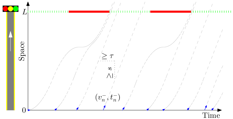
Roadway

Geometry: We consider a single-lane highway section of length $L$. Location on this segment starts from 0 at the upstream and ends at $L$ at the downstream. We use location set $[0,L]$ to denote this highway section. Traffic goes from location $0$ to $L$ on this section. A fixed-time traffic light is installed at location $L.$ The effective green phase starts at time $0$ with an duration of $G$, followed by an effective red phase of duration $R$, and this pattern continues all the way. This indicates the signal cycle time is always $C:=R+G$. We denote the set of green time intervals as $\mathcal{G}:=\left\{\left[g_{m}:=mC,r_{m}:=mC+G\right)\right\}_{m\in\mathbb{Z}^{+}}$ where $\mathbb{Z}^{+}$ is the non-negative integer set. We define function

$$G(t)=\min\{t^{\prime}\in\mathcal{G},t^{\prime}>t\},\forall t\in[-\infty,\infty],$$

which identifies the next closest green time to $t$. Note that $G(t)=t$ if $t\in\mathcal{G}$ or $G(t)>t$ if $t\notin\mathcal{G}$.

Vehicle

Characteristics: We consider a stream of $N$ identical automated vehicles indexed as $n\in\mathcal{N}:=\left\{1,2,\cdots,N\right\}$. Each vehicle’s acceleration at any time is no less than deceleration limit $\underline{a}<0$ and no greater than acceleration limit $\overline{a}>0$. The speed limit on this segment is $\bar{v}$, and we don’t allow a vehicle to back up, thus a vehicle’s speed range is $[0,\overline{v}]$.

We want to design a set of trajectories for these vehicles to follow on this highway section. A trajectory is formally defined below.

We let function $p_{n}$ denote the trajectory of vehicle $n,\forall n\in\mathcal{N}$. At any time $t$, $p_{n}(t)$ essentially denotes the location of vehicle $n$’s front bumper. Collectively we denote all vehicle trajectories by trajectory vector $\mathbf{p}:=\left[p_{n}(t)\right]_{n\in\mathcal{N}}$. The trajectories in vector $\mathbf{p}$ shall satisfy the following constraints.

Kinematic

Constraints: Trajectory $p$ is kinetically feasible if $\dot{p}(t)\in[0,\bar{v}]$ and $\ddot{p}(t)\in\left[\underline{a},\bar{a}\right],\forall t\in(-\infty,\infty)$. We denote the set of all kinetically feasible trajectories as

$$\mathcal{T}:=\left\{p\in\mathcal{\bar{T}}\left|0\leq\dot{p}(t)\leq\bar{v},\underline{a}\leq\ddot{p}(t)\leq\bar{a},\forall t\in\left(-\infty,\infty\right)\right.\right\}.$$

(1)

Entry

Boundary Condition: Let $t_{n}^{-}$ and $v_{n}^{-}$ denote the time and the speed when vehicle $n$ arrives at the entry of this segment (or location 0), $\forall n\in\mathcal{N}$. We require $t_{1}^{-}<t_{2}^{-}<\cdots<t_{N}^{-}$ and separation between $t_{n-1}$ and $t_{n}$ is sufficient for the safety requirement, $\forall n\in\mathcal{N}\backslash\{1\}$. Define the subset of trajectories in $\mathcal{T}$ that are consistent with vehicle $n$’s entry boundary condition as

$$\mathcal{T}_{n}^{-}:=\left\{p\in\mathcal{T}\left|p(t_{n}^{-})=0,\dot{p}(t_{n}^{-})=v_{n}^{-}\right.\right\},\forall n\in\mathcal{N}.$$

(2)

Exit

Boundary Condition: Due to the traffic signal at location $L$, vehicles can only exit this section during a green light. Denote the set of trajectories in $\mathcal{T}$ that pass location $L$ during a green signal phase by

$$\mathcal{T}^{+}:=\left\{p\in\mathcal{T}\left|p^{-1}(L)\in\mathcal{G}\right.\right\},\forall n\in\mathcal{N},$$

(3)

where the generalized inverse function is defined as $p^{-1}(l):=\inf\left\{t\left|p(t)\geq l\right.\right\},\forall l\in\left[0,\infty\right),p\in\mathcal{T}$. Note that function $p^{-1}(\cdot)$ shall satisfy the following properties:

P1: Function $p^{-1}(l)$ is increasing with $l\in\left(-\infty,\infty\right)$;

P2: Due to speed limit $\bar{v}$, $p^{-1}(l+\delta)\geq p^{-1}(l)+\delta/\bar{v},\forall l\in\left(-\infty,\infty\right),\delta\in[0,\infty)$.

Further, let $\mathcal{T}_{n}$ denote the set of trajectories that satisfy both vehicle $n$’s entry and exit boundary conditions, i.e., $\mathcal{T}_{n}=\mathcal{T}_{n}^{-}\bigcap\mathcal{T}^{+}$.

Car-following

Safety: We require that the separation between vehicle $n$’s location at any time and its preceding vehicle $(n-1$)’s location a communication delay $\tau$ ago is no less than a jam spacing $s$ (which usually includes the vehicle length and a safety buffer), $\forall n\in\mathcal{N}\backslash\{1\}$. For a genetic trajectory $p\in\mathcal{T}$ , a safely following trajectory of $p$ is a trajectory $p^{\prime}\in\mathcal{T}$ such that $p^{\prime}(t-\tau)-p(t)\geq s,\forall t\in(-\infty,\infty)$. We denote the set of all safely following trajectories of $p$ as $\mathcal{F}(p)$, i.e.,

$$\mathcal{F}(p):=\left\{p^{\prime}\left|p^{\prime}(t-\tau)-p(t)\geq s,\forall t\in(-\infty,\infty)\right.\right\},\forall p\in\mathcal{T}.$$

(4)

With this, we define $\mathcal{T}_{n}(p_{n-1}):=\mathcal{F}(p_{n-1})\bigcap\mathcal{T}_{n}$ that denotes the set of feasible trajectories for vehicle $n$ that are safely following given vehicle $(n-1)$’s trajectory $p_{n-1}$.

In summary, a feasible lead vehicle’s trajectory $p_{1}$ has to fall in $\mathcal{T}_{1}$, and any feasible following vehicle trajectory $p_{n}$ has to belong to $\mathcal{T}_{n}(p_{n-1}),\forall n\in\mathcal{N}\backslash\{1\}$ . We say a trajectory vector $\mathbf{p}$ is feasible if it satisfies all above-defined constraints. Let $\mathcal{P}$ denote the set of all feasible trajectory vectors, i.e.,

The primary problem (PP) investigated in this paper is finding and analyzing feasible solutions to $\mathcal{P}$.

In the classic traffic flow theory, the lead-vehicle problem (LVP) is a well-known fundamental problem that predicts traffic flow dynamics on one-lane freeway given the lead vehicle’s trajectory and the following vehicles’ initial states (Daganzo, 2006). We notice that PP (5) can be easily adapted to LVP by relaxing exit boundary condition (3) yet fixing trajectory $p_{1}$. The LVP is officially formulated as follows. Given lead vehicle’s trajectory $p_{1}\in\mathcal{T}$, the set of feasible trajectories for LVP is

The LVP investigated in this paper is finding and analyzing feasible solutions to $\mathcal{P}^{\mbox{LVP}}$.

This section presents a shooting heuristic (SH) algorithm that is able to construct a smooth and feasible trajectory vector to solve $\mathcal{P}$ in PP very efficiently. Traditional methods for trajectory optimization include analytical approaches that can only solve simple problems with special structures and numerical approaches that can accommodate more complex settings yet may demand enormous computation resources (Von Stryk and Bulirsch, 1992). Since a vehicle trajectory is essentially an infinite-dimensional object along which the state (e.g. location, speed, acceleration) at every point can be varied, it is challenging to even construct one single trajectory, particularly under nonlinear constraints. Note that our problem deals with a large number of trajectories for vehicles in a traffic stream that constantly interact with each other and are subject to complex nonlinear constraints (1)-(5). Therefore we deem that it is very complex and time-consuming to tackle this problem with a traditional approach. Therefore, we opt to devise a new approach that circumvents the need for formulating high-dimensional objects or complex system constraints. This leads to the development of a shooting heuristic (SH) algorithm that can efficiently construct a smooth feasible trajectory vector with only a few control parameters.

Figure 3 illustrates the components in the proposed SH algorithm. Basically, for each vehicle $n\in\mathcal{N}$, SH first constructs a trajectory, denoted by $p_{n}^{\mbox{f}}$ , with a forward shooting process that conforms with kinematic constraint (1), entry boundary constraint (2) and safety constraint (4) (if $n>1$). As illustrated in Figure 3(a), if trajectory $p_{n}^{\mbox{f}}$ (dashed blue curve) turns out far enough from preceding trajectory $p_{n-1}$ (red solid curve) such that safety constraint (4) is even not activated (or if $n=1$ and $p_{n}^{\mbox{f}}$ is already the lead trajectory), $p_{n}^{\mbox{f}}$ basically accelerates from its entry boundary condition $\left(t_{n}^{-},v_{n}^{-}\right)$ at location 0 with a forward acceleration rate of $\bar{a}^{\mbox{f}}\in(0,\bar{a}]$ until reaching speed limit $\bar{v}$ and then cruises at constant speed $\bar{v}$. Otherwise, as illustrated in Figure 3(b), if trajectory $p_{n}^{\mbox{f}}$ is blocked by $p_{n-1}$ due to safety constraint (4), we just let $p_{n}^{\mbox{f}}$ smoothly merge into a safety bound (the red dotted curve) translated from $p_{n-1}$ that just keeps spatial separation $s$ and temporal separation $\tau$ from $p_{n}^{\mbox{f}}$. The transitional segment connecting $p_{n}^{\mbox{f}}$ with the safety bound decelerates at a forward deceleration rate of $\underline{a}^{\mbox{f}}\in[\underline{a},0)$. If trajectory $p_{n}^{\mbox{f}}$ from the forward shooting process is found to violate exit boundary constraint (3) (or run into the red light), as illustrated in Figure 3(c), a backward shooting process is activated to revise $p_{n}^{\mbox{f}}$ to comply with constraint (3). The backward shooting process first shifts the section of $p_{n}^{\mbox{f}}$ above location $L$ rightwards to the start of the next green phase to be a backward shooting trajectory $p_{n}^{\mbox{b}}$ . Then $p_{n}^{\mbox{b}}$ shoots backwards from this start point at a backward acceleration rate $\bar{a}^{\mbox{b}}\in(0,\bar{a}]$ until getting close enough to merge into $p_{n}^{\mbox{f}}$ , which may require $p_{n}^{\mbox{b}}$ stops for some time if the separation between the backward shooting start point and $p_{n}^{\mbox{f}}$ is long relative to acceleration rate $\bar{a}^{\mbox{b}}$ . Then, $p_{n}^{\mbox{b}}$ shoots backwards a merging segment at a backward deceleration rate of $\underline{a}^{\mbox{b}}\in[\underline{a},0)$ until getting tangent to $p_{n}^{\mbox{f}}$. Finally, merging $p_{n}^{\mbox{f}}$ and $p_{n}^{\mbox{b}}$ yields a feasible trajectory $p_{n}$ for vehicle $n$. Such forward and backward shooting processes are executed from vehicle $1$ through vehicle $N$ consecutively, and then SH concludes with a feasible trajectory vector $\mathbf{p}=\left[p_{n}\right]{}_{n\in\mathcal{N}}\in\mathcal{P}.$ Note that SH only uses four control variables $\left\{\bar{a}^{\mbox{f}},\underline{a}^{\mbox{f}},\bar{a}^{\mbox{b}},\underline{a}^{\mbox{b}}\right\}$ that are yet able to control the overall smoothness of all trajectories (so as to achieve certain desired objectives). Further, the constructed trajectories are composed of only a few quadratic (or linear) segments that are all analytically solvable. Therefore, the proposed SH algorithm is parsimonious and simple to implement.

To formally state SH, we first define the following terminologies in Definitions 2-4 with respect to a single trajectory, as illustrated in Figure 4(a).

During the forward shooting process, we need to check safety constraints (4) at every move for any vehicle $n\geq 2$. As illustrated in Figure 4(b), we basically create a shadow (or safety bound) of the preceding trajectory $p_{n-1}$ by shifting $p_{n-1}$ downwards by $s$ and rightwards by $\tau$. Then safety constraint (4) is simply equivalent to that $p_{n}$ does not exceed this shadow trajectory at any time. The following definition specifies the shadow trajectory and its elemental segments.

The following definitions specify an analytical function that checks the distance between two segments (e.g., the current segment to be constructed and a reference shadow segment in forward shooting), as illustrated in Figure 4(c).

FSO-1:

If $D\left(\mathbf{s}^{\prime}-\bar{\mathbf{s}}\right)<0$ where $\bar{\mathbf{s}}:=\left(l,v,a^{-},t^{-},\infty\right)$, there is no feasible solution, and we just set $t^{\mbox{m}}=t^{+}=-\infty$ (Case I). Go to Step FSO-3.

FSO-2:

Shift the origin to time $t^{-}$ and denote $\hat{t}^{\prime-}:=t^{\prime-}-t^{-}$, $\hat{t}^{\prime+}:=t^{\prime+}-t^{-}$, $\hat{t}^{\mbox{m}}:=t^{\mbox{m}}-t^{-}$, $\hat{t}^{\mbox{+}}:=t^{\mbox{+}}-t^{-}$ and $\hat{t}^{-}:=\max\{\hat{t}^{\prime-},0\}$. Then get a quadratic function $\mathbf{q}$ by subtracting $\left(l^{\mbox{m}},v^{\mbox{m}},a^{-},t^{\mbox{m}}\right)$ from $(l^{\prime},v^{\prime},a^{\prime},t^{\prime-})$, i.e., $\mathbf{q}:=\left(\hat{l},\hat{v},a^{\prime}-a^{-},0\right)$ where

$$\hat{l}:=0.5a^{\prime}\left(\hat{t}^{\prime-}\right)^{2}+0.5\left(a^{+}-a^{-}\right)\left(\hat{t}^{\mbox{m}}\right)^{2}-a^{\prime}\hat{t}^{\prime-}+l^{\prime}-l,$$

and

$$\hat{v}=v^{\prime}-v-a^{\prime}\hat{t}^{\prime-}-\left(a^{+}-a^{-}\right)\hat{t}^{\mbox{m}}.$$

FSO-2-1:

If $a^{\prime}=a^{-}$, test whether we can make $\mathbf{q}(t)=0,\forall t\in[\hat{t}^{-},\infty)$, i.e., whether $\hat{l}=0$ with $\hat{t}^{\mbox{m}}=\left(v^{\prime}-v-a^{\prime}\hat{t}^{\prime-}\right)/\left(a^{+}-a^{-}\right)$. If yes and $\hat{t}^{\mbox{m}}\in\left[\hat{t}^{-},\hat{t}^{\prime+}\right]$ (Case II), set $t^{\mbox{m}}=t^{-}+\hat{t}^{\mbox{m}}$ and $t^{\mbox{+}}=t^{\prime+}$. Otherwise (Case III), set $t^{\mbox{+}}=t^{\mbox{m}}=\infty$. Go to Step FSO-3.

FSO-2-2:

If $a^{{}^{\prime}}>a^{-}$,then $\mathbf{q}$ is a convex quadratic function, and we need to solve $\alpha\left(\hat{t}^{\mbox{m}}\right)^{2}+\beta\hat{t}^{\mbox{m}}+\gamma=0$ where $\alpha:=\left(a^{+}-a^{-}\right)\left(a^{+}-a^{\prime}\right)$, $\beta:=-2\left(a^{+}-a^{-}\right)\left(v^{\prime}-v-a^{\prime}\hat{t}^{\prime-}\right)$ and $\gamma:=\left(v^{\prime}-v-a^{\prime}\hat{t}^{\prime-}\right)^{2}-(a^{\prime}-a^{-})\left(a^{\prime}\left(\hat{t}^{\prime-}\right)^{2}-2v^{\prime}\hat{t}^{\prime-}+2l^{\prime}-2l\right)$ . In case of $\alpha=\beta=0$ (Case III), set $t^{\mbox{+}}=t^{\mbox{m}}=\infty$, and go to Step FSO-3. Otherwise, we need to try candidate solutions to $\hat{t}^{\mbox{m}}$ and $\hat{t}^{\mbox{+}}$, denoted by $\hat{t}^{\mbox{mc}}$ and $\hat{t}^{+\mbox{c}}$, respectively. In case of $\alpha=0$ but $\beta\neq 0$, solve $\hat{t}^{\mbox{mc}}=-\gamma/\beta$ and

$$\hat{t}^{+\mbox{c}}=\frac{v^{\prime}-v-a^{\prime}\hat{t}^{\prime-}-\left(a^{+}-a^{-}\right)\hat{t}^{\mbox{mc}}}{a^{-}-a^{\prime}}.$$

(9)

Otherwise, we should have $\alpha\neq 0$, and then solve both candidate solutions

$$\hat{t}^{\mbox{mc}}=\frac{-\beta\pm\sqrt{\beta^{2}-4\alpha\gamma}}{2\alpha}$$

(10)

and the corresponding $\hat{t}^{+\mbox{c}}$ with equation(9). If the candidate solutions are not real numbers, then we just set $\hat{t}^{\mbox{+c}}=\hat{t}^{\mbox{mc}}=\infty$. Otherwise, try both sets of solutions and select the set satisfying $\hat{t}^{+\mbox{c}}\geq\hat{t}^{\mbox{mc}}\geq 0$. For either of these two cases, if $\hat{t}^{+\mbox{c}}\in\left[\hat{t}^{-},\hat{t}^{\prime+}\right]$ (Case II) , we set $t^{\mbox{m}}=t^{-}+\hat{t}^{\mbox{mc}}$ and $\hat{t}^{\mbox{+}}=\hat{t}^{\mbox{+c}}$. Otherwise, set $t^{\mbox{+}}=t^{\mbox{m}}=\infty$ (Case III). Go to Step FSO-3.

FSO-3:

Finally, we return $t^{\mbox{mf}}\left(\mathbf{s}^{\prime},\left(l,v,t^{-},a^{+}\right),a^{-}\right)=t^{\mbox{m}}$ and $t^{\mbox{+f}}\left(\mathbf{s}^{\prime},\left(l,v,t^{-},a^{+}\right),a^{-}\right)=t^{\mbox{+}}$.

FSP-1:

Initiate $h=1$, $t^{+}=t^{\mbox{m}}=\infty$, $p^{\mbox{f}}=\emptyset$ and iterate through the segments in $p^{\mbox{s}}$ as follows.

FSP-2:

If $v<\bar{v}$, apply the FSO algorithm to solve candidate time points $t^{\mbox{mc}}:=t^{\mbox{mf}}\left(\mathbf{s}_{h}^{\mbox{s}},(l,v,\bar{a}^{\mbox{f}},t^{-}),\underline{a}^{\mbox{f}}\right)$ and $t^{+\mbox{c}}:=t^{\mbox{+f}}\left(\mathbf{s}_{h}^{\mbox{s}},(l,v,\bar{a}^{\mbox{f}},t^{-}),\underline{a}^{\mbox{f}}\right)$. If $t^{\mbox{mc}}>t^{\mbox{a}}$, revise $t^{\mbox{mc}}:=(t^{\mbox{mf}}\mathbf{s}_{h}^{\mbox{s}},(l^{\mbox{a}},\bar{v},0,t^{\mbox{a}}),\underline{a}^{\mbox{f}})$ and $t^{\mbox{+c}}:=t^{\mbox{+f}}(\mathbf{s}_{h}^{\mbox{s}},(l^{\mbox{a}},\bar{v},0,t^{\mbox{a}}),\underline{a}^{\mbox{f}})$. If $v=\bar{v}$, solve $t^{\mbox{mc}}:=t^{\mbox{mf}}(\mathbf{s}_{h}^{\mbox{s}},(l,\bar{v},0,t^{-}),\underline{a}^{\mbox{f}})$ and $t^{\mbox{+c}}:=(t^{\mbox{+f}}\mathbf{s}_{h}^{\mbox{s}},(l,\bar{v},0,t^{-}),\underline{a}^{\mbox{f}})$. If $t^{\mbox{mc}}=-\infty$, the algorithm cannot find a feasible solution and return $p^{\mbox{f}}((l,v,t^{-}),p^{\mbox{s}})=\emptyset$, $t^{\mbox{mf}}((l,v,t^{-}),p^{\mbox{s}})=-\infty$ and $t^{+\mbox{f}}((p,v,t^{-}),p^{\mbox{s}})=-\infty$. If $t^{\mbox{+c}}\in[t_{h}^{\mbox{s}},t_{h+1}^{\mbox{s}}]$, set $t^{\mbox{m}}=t^{\mbox{mc}}$ and $t^{+}=t^{+\mbox{c}}$, and go to the Step FSP-3. Otherwise, $t^{\mbox{+c}}$ shall be $\infty$. Then if $h<\bar{h}$, set $h=h+1$ and repeat this step.

FSP-3:

If $v<\bar{v}$ and $t^{\mbox{a}}>t^{-}$, append segment $(l,v,\bar{a}^{\mbox{f}},t^{-},\min(t^{\mbox{m}},t^{\mbox{a}}))$ to $p^{\mbox{f}}$ (appending means adding this segment as the last element of $p^{\mbox{f}}$). If $t^{\mbox{m}}>t^{\mbox{a}},$ append $(l^{\mbox{a}},\bar{v},0,t^{\mbox{a}},t^{\mbox{m}})$ to $p^{\mbox{f}}$. If $t^{+}<t_{\bar{h}+1}^{\mbox{s}}$, which indicates $t^{+}\in[t_{h}^{\mbox{s}},t_{h+1}^{\mbox{s}}]$, we first append segment $(l_{h}^{\mbox{s}}+v_{h}^{\mbox{s}}(t^{+}-t_{h}^{\mbox{s}})+0.5a_{h}^{\mbox{s}}(t^{+}-t_{h}^{\mbox{s}})^{2},v_{h}^{\mbox{s}}+a_{h}^{\mbox{s}}(t^{+}-t_{h}^{\mbox{s}}),a_{h}^{\mbox{s}},t^{+},t_{h+1}^{\mbox{s}})$ to $p^{\mbox{f}}$, and then append all segments $[\mathbf{s}_{h^{\prime}}^{\mbox{s}}]_{h^{\prime}=h+1,\cdots,\bar{h}}$ to $p^{\mbox{f}}$.

FSP-4:

Finally, return $p^{\mbox{f}}((l,v,t^{-}),p^{\mbox{s}})=p^{\mbox{f}}$, $t^{\mbox{mf}}((l,v,t^{-}),p^{\mbox{s}})=t^{\mbox{m}}$ and $t^{+\mbox{f}}((p,v,t^{-}),p^{\mbox{s}})=t^{+}$.

References

- Ahn et al. [2013] Ahn, K., Rakha, H., Park, S., 2013. Ecodrive application: Algorithmic development and preliminary testing. Transportation Research Record: Journal of the Transportation Research Board (2341), 1–11.
- Ahn [2005] Ahn, S., 2005. Formation and spatial evolution of traffic oscillations. Ph.D. thesis, University of California, Berkeley, Berkeley, California.
- Apostol [1969] Apostol, T. M., 1969. Calculus, vol. ii. Ed Reverté.
- Bando et al. [1998] Bando, M., Hasebe, K., Nakanishi, K., Nakayama, A., 1998. Analysis of optimal velocity model with explicit delay. Physical Review E 58 (5), 5429–5435.
- Bando et al. [1995] Bando, M., Hasebe, K., Nakayama, A., Shibata, A., Sugiyama, Y., 1995. Dynamical model of traffic congestion and numerical simulation. Physical Review E 51 (2), 1035–1042.
- Beard and Griffin [2013] Beard, G. F., Griffin, M. J., 2013. Discomfort during lateral acceleration: Influence of seat cushion and backrest. Applied ergonomics 44 (4), 588–594.
- Bham et al. [2010] Bham, G. H., Long, S., Baik, H., Ryan, T., Gentry, L., Lall, K., Arezoumandi, M., Liu, D., Li, T., Schaeffer, B., 2010. Evaluation of variable speed limits on i-270/i-255 in st. louis. Tech. rep.
- Brackstone and McDonald [1999] Brackstone, M., McDonald, M., 1999. Car-following: a historical review. Transportation Research Part F: Traffic Psychology and Behaviour 2 (4), 181 – 196.
- Cassidy and Bertini [1999] Cassidy, M., Bertini, R., 1999. Some traffic features at freeway bottlenecks. Transportation Research Part B 33 (1), 25–42.
- Chandler et al. [1958] Chandler, R. E., Herman, R., Montroll, E. W., 1958. Traffic dynamics: Studies in car following. Operations Research 6 (2), 165–184.
- Daganzo [1994] Daganzo, C. F., 1994. The cell transmission model: A dynamic representation of highway traffic consistent with the hydrodynamic theory. Transportation Research Part B: Methodological 28 (4), 269 – 287.
- Daganzo [2006] Daganzo, C. F., 2006. In traffic flow, cellular automata=kinematic waves. Transportation Research Part B: Methodological 40 (5), 396 – 403.
- Daganzo et al. [1999] Daganzo, C. F., Cassidy, M. J., Bertini, R. L., 1999. Possible explanations of phase transitions in highway traffic. Transportation Research Part A: Policy and Practice 33 (5), 365–379.
- De Nunzio et al. [2013] De Nunzio, G., Canudas de Wit, C., Moulin, P., Di Domenico, D., 2013. Eco-driving in urban traffic networks using traffic signal information. In: Decision and Control (CDC), 2013 IEEE 52nd Annual Conference on. IEEE, pp. 892–898.
- Dresner and Stone [2008] Dresner, K., Stone, P., 2008. A multiagent approach to autonomous intersection management. Journal of Artificial Intelligence Research 31, 591–656.
- Guan and Frey [2013] Guan, T., Frey, C. W., 2013. Predictive fuel efficiency optimization using traffic light timings and fuel consumption model. In: Intelligent Transportation Systems-(ITSC), 2013 16th International IEEE Conference on. IEEE, pp. 1553–1558.
- Hegyi et al. [2005] Hegyi, A., De Schutter, B., Hellendoorn, H., 2005. Model predictive control for optimal coordination of ramp metering and variable speed limits. Transportation Research Part C: Emerging Technologies 13 (3), 185–209.
- Herman et al. [1958] Herman, R., Montroll, E. W., Potts, R. B., Rothery, R. W., 1958. Traffic dynamics: Analysis of stability in car following. Operations Research 7 (1), 86–106.
- Hoffmann and Mortimer [1994] Hoffmann, E. R., Mortimer, R. G., 1994. Drivers’ estimates of time to collision. Accident Analysis & Prevention 26 (4), 511–520.
- Hooker [1988] Hooker, J., 1988. Optimal driving for single-vehicle fuel economy. Transportation Research Part A: General 22 (3), 183–201.
- Iglesias et al. [2008] Iglesias, I., Isasi, L., Larburu, M., Martinez, V., Molinete, B., 2008. I2v communication driving assistance system: on-board traffic light assistant. In: Vehicular Technology Conference, 2008. VTC 2008-Fall. IEEE 68th. IEEE, pp. 1–5.
- Islam et al. [2013] Islam, M., Hadiuzzaman, M., Fang, J., Qiu, T., El-Basyouny, K., 2013. Assessing mobility and safety impacts of a variable speed limit control strategy. Transportation Research Record: Journal of the Transportation Research Board (2364), 1–11.
- Kamalanathsharma et al. [2013] Kamalanathsharma, R. K., Rakha, H., et al., 2013. Multi-stage dynamic programming algorithm for eco-speed control at traffic signalized intersections. In: Intelligent Transportation Systems-(ITSC), 2013 16th International IEEE Conference on. IEEE, pp. 2094–2099.
- Kerner [1998] Kerner, B., 1998. Experimental features of self-organization in traffic flow. Physical Review Letter 81 (17), 3797–3800.
- Kerner and Rehborn [1996] Kerner, B., Rehborn, H., 1996. Experimental properties of complexity in traffic flow. Physical Review E 53 (5), R4275–R4278.
- Kerner and Rehborn [1997] Kerner, B. S., Rehborn, H., 1997. Experimental properties of phase transitions in traffic flow. Physical Review Letters 79 (20), 4030–4033.
- Kuhne [1987] Kuhne, R. D., 1987. Freeway speed distribution and acceleration noise. In: Gartner, N. H., Wilson, N. H. (Eds.), Proceedings of the 10th International Symposium on Transportation and Traffic Theory. pp. 119–137.
- Laval [2011a] Laval, J. A., 2011a. Hysteresis in traffic flow revisited: An improved measurement method. Transportation Research Part B 45 (2), 385 – 391.
- Laval [2011b] Laval, J. A., 2011b. Hysteresis in traffic flow revisited: An improved measurement method. Transportation Research Part B 45 (2), 385 – 391.
- Lee and Park [2012a] Lee, J., Park, B., 2012a. Development and evaluation of a cooperative vehicle intersection control algorithm under the connected vehicles environment. Intelligent Transportation Systems, IEEE Transactions on 13 (1), 81–90.
- Lee and Park [2012b] Lee, J., Park, B., 2012b. Development and evaluation of a cooperative vehicle intersection control algorithm under the connected vehicles environment. Intelligent Transportation Systems, IEEE Transactions on 13 (1), 81–90.
- Li et al. [2014] Li, X., Cui, J., An, S., Parsafard, M., 2014. Stop-and-go traffic analysis: Theoretical properties, environmental impacts and oscillation mitigation. Transportation Research Part B: Methodological 70, 319–339.
- Li and Ouyang [2011] Li, X., Ouyang, Y., 2011. Characterization of traffic oscillation propagation under nonlinear car-following laws. Transportation Research Part B 45 (9), 1346–1361.
- Lighthill and Whitham [1955] Lighthill, M. J., Whitham, G. B., 1955. On Kinematic Waves. II. A Theory of Traffic Flow on Long Crowded Roads. Royal Society of London Proceedings Series A 229, 317–345.
- Liu et al. [2012] Liu, B., Ghosal, D., Chuah, C.-N., Zhang, H. M., 2012. Reducing greenhouse effects via fuel consumption-aware variable speed limit (fc-vsl). Vehicular Technology, IEEE Transactions on 61 (1), 111–122.
- Lu and Shladover [2014] Lu, X.-Y., Shladover, S., 2014. Review of variable speed limits and advisories: Theory, algorithms, and practice. Transportation Research Record: Journal of the Transportation Research Board (2423), 15–23.
- Ma et al. [2015] Ma, J., Li, X., Zhou, F., Hu, J., Park, B., 2015. A parsimonious two-way shooting algorithm for connected automated traffic smoothing part ii: Optimization framework. Working paper, Mississippi State University.
- Mandava et al. [2009] Mandava, S., Boriboonsomsin, K., Barth, M., 2009. Arterial velocity planning based on traffic signal information under light traffic conditions. In: Intelligent Transportation Systems, 2009. ITSC’09. 12th International IEEE Conference on. IEEE, pp. 1–6.
- Mauch and Cassidy [2002] Mauch, M., Cassidy, M., 2002. Freeway traffic oscillations: observations and predictions. In: Taylor, M. A. (Ed.), Proceedings of the 15th International Symposium on Transportation and Traffic Theory. pp. 653–674.
- Miller [2005] Miller, H. J., 2005. A measurement theory for time geography. Geographical analysis 37 (1), 17–45.
- Nagel and Schreckenberg [1992] Nagel, K., Schreckenberg, M., 1992. A cellular automaton model for freeway traffic. Journal de Physique I 2 (12), 2221–2229.
- Newell [1993] Newell, G. F., 1993. A simplified theory of kinematic waves in highway traffic, part i: general theory. Transportation Research Part B: Methodological 27 (4), 281–287.
- Newell [2002] Newell, G. F., 2002. A simplified car-following theory: a lower order model. Transportation Research Part B 36 (3), 195 – 205.
- Rakha and Kamalanathsharma [2011] Rakha, H., Kamalanathsharma, R. K., 2011. Eco-driving at signalized intersections using v2i communication. In: Intelligent Transportation Systems (ITSC), 2011 14th International IEEE Conference on. IEEE, pp. 341–346.
- Richards [1956] Richards, P. I., 1956. Shock Waves on the Highway . Operations Research 4 (1), 42–51.
- Sanchez et al. [2006] Sanchez, M., Cano, J.-C., Kim, D., 2006. Predicting traffic lights to improve urban traffic fuel consumption. In: 2006 6th International Conference on ITS Telecommunications.
- Schwarzkopf and Leipnik [1977] Schwarzkopf, A., Leipnik, R., 1977. Control of highway vehicles for minimum fuel consumption over varying terrain. Transportation Research 11 (4), 279–286.
- Shladover et al. [2009] Shladover, S. E., Nowakowski, C., Cody, D., Bu, F., O′Connell, J., Spring, J., Dickey, S., Nelson, D., 2009. Effects of cooperative adaptive cruise control on traffic flow: Testing drivers′ choices of following distances. Tech. Rep. UCB-ITS-PRR-2009-23, California PATH, Berkeley, CA.
- Spiliopoulou et al. [2009] Spiliopoulou, A. D., Papamichail, I., Papageorgiou, M., 2009. Toll plaza merging traffic control for throughput maximization. Journal of Transportation Engineering 136 (1), 67–76.
- Tielert et al. [2010] Tielert, T., Killat, M., Hartenstein, H., Luz, R., Hausberger, S., Benz, T., 2010. The impact of traffic-light-to-vehicle communication on fuel consumption and emissions. In: Internet of Things (IOT), 2010. IEEE, pp. 1–8.
- Trayford et al. [1984a] Trayford, R., Doughty, B., van der Touw, J., 1984a. Fuel economy investigation of dynamic advisory speeds from an experiment in arterial traffic. Transportation Research Part A: General 18 (5), 415–419.
- Trayford et al. [1984b] Trayford, R., Doughty, B., Wooldridge, M., 1984b. Fuel saving and other benefits of dynamic advisory speeds on a multi-lane arterial road. Transportation Research Part A: General 18 (5), 421–429.
- Treiber et al. [2000] Treiber, M., Hennecke, A., Helbing, D., 2000. Congested traffic states in empirical observations and microscopic simulations. Physical Review E 62 (2), 1805–1824.
- Treiber et al. [2010] Treiber, M., Kesting, A., Helbing, D., 2010. Three-phase traffic theory and two-phase models with a fundamental diagram in the light of empirical stylized facts. Transportation Research Part B: Methodological 44 (8), 983–1000.
- Van Arem et al. [2006] Van Arem, B., van Driel, C., Visser, R., 2006. The impact of cooperative adaptive cruise control on traffic-flow characteristics. Intelligent Transportation Systems, IEEE Transactions on 7 (4), 429–436.
- Von Stryk and Bulirsch [1992] Von Stryk, O., Bulirsch, R., 1992. Direct and indirect methods for trajectory optimization. Annals of operations research 37 (1), 357–373.
- Wang et al. [2014a] Wang, M., Daamen, W., Hoogendoorn, S. P., van Arem, B., 2014a. Rolling horizon control framework for driver assistance systems. part i: Mathematical formulation and non-cooperative systems. Transportation Research Part C: Emerging Technologies 40, 271–289.
- Wang et al. [2014b] Wang, M., Daamen, W., Hoogendoorn, S. P., van Arem, B., 2014b. Rolling horizon control framework for driver assistance systems. part ii: Cooperative sensing and cooperative control. Transportation Research Part C: Emerging Technologies 40, 290–311.
- Wu et al. [2010] Wu, G., Boriboonsomsin, K., Zhang, W.-B., Li, M., Barth, M., 2010. Energy and emission benefit comparison of stationary and in-vehicle advanced driving alert systems. Transportation Research Record: Journal of the Transportation Research Board (2189), 98–106.
- Wu et al. [2015] Wu, X., He, X., Yu, G., Harmandayan, A., Wang, Y., 2015. Energy-optimal speed control for electric vehicles on signalized arterials. Intelligent Transportation Systems, IEEE Transactions on PP (99), 1–11.
- Yang and Jin [2014] Yang, H., Jin, W.-L., 2014. A control theoretic formulation ofgreen driving strategies based on inter-vehicle communications. Transportation Research Part C: Emerging Technologies 41, 48–60.
- Zohdy and Rakha [2014] Zohdy, I. H., Rakha, H. A., 2014. Intersection management via vehicle connectivity: The intersection cooperative adaptive cruise control system concept. Journal of Intelligent Transportation Systems (ahead-of-print), 1–16.