Minimax wavelet estimation for multisample heteroscedastic non-parametric regression
Abstract
The problem of estimating the baseline signal from multisample noisy curves is investigated. We consider the functional mixed effects model, and we suppose that the functional fixed effect belongs to the Besov class. This framework allows us to model curves that can exhibit strong irregularities, such as peaks or jumps for instance. The lower bound for the minimax risk is provided, as well as the upper bound of the minimax rate, that is derived by constructing a wavelet estimator for the functional fixed effect. Our work constitutes the first theoretical functional results in multisample non parametric regression. Our approach is illustrated on realistic simulated datasets as well as on experimental data.
keywords.-functional mixed effects models; minimax risk; Besov class; wavelet estimator;
1 Introduction
Functional data analysis has gained increased attention in the past years, in particular in high-throughput biology with the use of mass spectrometry. In this field, the signal is a spectrum whose peaks provide information regarding the protein content of biological samples. A new challenge in functional data analysis is the availability of multisample data for which functional ANOVA has become the appropriate framework. More specifically for spectrometry data, it is now well accepted that the noise corrupting the signal can be divided into a technical white noise added to an important inter-individual variability (Eckel-Passow et al., 2009). In this case, the usual non-parametric regression framework (a deterministic trend corrupted by a random noise) is no longer appropriate since it does not account for heteroscedastic noise structure. Functional mixed effects models (Antoniadis and Sapatinas, 2007) appear to be a powerful framework to handle these data, as others, and we focus here on the estimation of the baseline signal.
In practice, a trivial averaging procedure is often used to get an estimate of the baseline signal, but it has both a poor convergence rate and a finite sample performance. Amato and Sapatinas (2005) proposed an approach for baseline estimation based on empirical wavelet coefficients of the observed data. Unfortunately the convergence of their estimator is not theoretically assessed, and more broadly, there is a general lack of theoretical results on functional estimators in functional mixed models, despite their increasing importance in practice (Morris and Carroll, 2006; Morris et al., 2008).
In this work we propose a minimax estimator of the baseline signal, based on the empirical wavelet coefficients of the observed data. The functional fixed effect is assumed to belong to the Besov class, which allows us to model curves that can exhibit strong irregularities, such as peaks in mass spectrometry data. We construct the lower bound for the minimax risk. This convergence rate is the same as in the classical non parametric setting but with an additional approximation error term. Then, we propose a wavelet estimator that achieves near optimal rate of convergence (within a logarithmic factor in sample size). Through simulation studies, we show that our approach outperforms the approach proposed by Amato and Sapatinas (2005). We also propose a new thresholding procedure based on the Stein Unbiased Risk Estimate (SURE) (Stein, 1981), combined with the SCAD thresholding (Antoniadis and Fan, 2001). This leads to improved performance for the baseline signal estimation.
This article is organized as follows. Section 2 presents the heteroscedastic model and the theoretical properties of our minimax estimator (lower and upper bounds). In particular we show how classical rates are modified in the presence of replicates along with inter-individual variability. Most of all, our work constitutes the first theoretical functional results in heteroscedastic multisample non-parametric regression. Several thresholding strategies are considered in Section 3, where we provide a new SURE-based procedure. Section 4 is devoted to the numerical experiments, and the procedure is illustrated on an experimental dataset. Technical proofs are provided in the Appendix.
2 Heteroscedastic nonparametric regression model and theoretical properties
2.1 Functional model
We observe curves , for over equally spaced time points in , with for some integer . In the general functional setting we consider a functional modeling (as in Antoniadis and Sapatinas (2007)) for the observed signal of the th individual:
| (1) |
where , for are stochastically independent random functions that are modeled as realizations of zero-mean Gaussian processes with parametrically structured covariances modeled in the wavelet domain (see Section 2.4). We define to be the main functional fixed effect characterizing a population average profile. In the following, we will denote by , , the vector of observations on the time grid, and similarly by and , , respectively the vector of the fixed effect and the noise terms, observed on the discrete time grid.
This modeling allows us to account for functional mixed effects models by decomposing in a sum of two independent processes , where are independent and identically distributed Gaussian random variables with zero-mean and constant variance; is a centered Gaussian process standing for subject-specific functional deviations. In Amato and Sapatinas (2005), the authors introduce similar model although the variance of the process is constant with respect to positions .
2.2 Minimax approach
In what follows we suppose that belongs to the Besov class (see Section 2.4 for a proper definition), a set of compactly supported functions (on ) with a bounded Besov space norm (by ). Such a set allows to model curves that can exhibit strong irregularities, such as peaks or jumps for instance. The notion of regularity is at the core of the functional setting which makes inhomogeneous Besov spaces a privileged tool for irregular function analysis. These spaces allow the fine definition of the regularity of a function along with its derivatives lying in while bringing a correction to this regularity. For a detailed review of Besov spaces and their properties, we refer the reader to the books of Härdle et al. (1998) or DeVore and Lorentz (1993).
Our goal is to recover the main functional effect from noisy observations. An originality of our approach is to consider multiple, say , individuals, which constitute available replicates to estimate the main fixed effect. To derive our estimator, we propose to use the so-called minimax approach. In this setup the risk of an estimator is defined by , with being a functional norm or a semi-norm. Then the so-called minimax estimator, denoted by , is the minimizer of the maximal risk on class over the set of all estimators:
Thus the challenge is to propose an optimal minimax estimator , and to derive its associated risk , also referred to as the minimax risk.
The construction of minimax estimators on the Besov classes is well known when only one replicate is available (see Härdle et al. (1998)). When errors are measured with a -norm “sharper” than the norm of the functional class , wavelet-based thresholding estimators can significantly outperform linear projection estimates. The rate of convergence depends on , and with two zones: the regular zone with usual rate and the sparse zone with a slower rate of convergence. However, this rate is not known when replicates are available (). In this work we establish this risk for (we will denote this norm by ) and for the Besov class with usual constraints , and . That leads to consider the regular zone since, in this case, we have (see Härdle et al. (1998)). In order to establish the minimax risk, we first give its lower bound and secondly we propose an estimator that achieves a near optimal rate of convergence. In this context, the near-optimality means that the minimax rate is attained within a logarithmic factor in sample size .
2.3 Lower bound for the minimax risk
One of the main contributions of this paper is to derive the asymptotic lower and upper bounds for . The following theorem gives the lower bound for this minimax risk in the inhomogeneous Besov class when dealing with multisample datasets ( ).
Theorem 2.1
Under the model (1) with finite variances for the processes , for assume that belongs to a Besov class with , , and , then
where if otherwise.
Let us mention that the term could be expected since it is the minimax rate (when ) considering a noise of variance . However the approximation error term , present in the case with only one sample (), is always negligible compared with the term . When , even a large does not provide more information on the function outside the grid . Hence, becomes a limiting term.
2.4 Wavelet estimator of the functional effect
The upper bound of the minimax rate given in Theorem 2.1 is derived by constructing a wavelet estimator of . Owing to their strong connection with the class of Besov spaces, wavelets indeed represent a powerful tool to perform adaptive functional regression (see Donoho et al. (1995)).
As a brief recall and to set notations, wavelets can be used to construct orthonormal basis of the functional Hilbert space by dilating and translating a compactly supported scaling function denoted by and a compactly supported mother wavelet denoted by . We assume that and belongs to Then, letting be the first level of approximation, the family:
with and is an orthonormal basis of . Thus, any function in the space can be expressed in the wavelet basis as:
where and are respectively the theorical approximation and wavelet coefficients, and with being the canonical Hilbertian scalar product associated with the space . In the following, we set and omit the index for the unique remaining scaling coefficient denoted by .
The Besov class is defined via wavelet coefficients in the following way:
where
For and the norm is equivalent to the norm of the corresponding Besov space (cf. Donoho (1994), Delyon and Juditsky (1997)).
In statistical settings, we are more concerned with discretely sampled curves. By applying the fast discrete wavelet transform proposed by Mallat (1989) to the functional model (1), we obtain a representation of the model in the coefficient domain given by:
| (2) |
The vector contains scaling and wavelet coefficients associated with the signal, while stand for empirical coefficients related to the fixed effect and for the coefficients coming from the error term . Following Antoniadis and Sapatinas (2007), the modeling of such correlated noise is performed directly in the wavelet domain by assuming first that is a diagonal matrix thanks to the well known decorrelating property of wavelets (see Frazier et al. (1991)). Then, to attain a wide range of processes, variances are assumed to vary with respect to the position and the resolution level such that and for all in with . Conversely, existing works dealing with a correlated noise focused on the modeling of individual noise processes in the time domain by assuming a stationnary noise (Johnstone and Silverman (1997)) or a locally stationnary noise (von Sachs and MacGibbon (2000)). In the wavelet domain these assumptions translate into variance terms for the matrix that are respectively depending on () or depending on both and . Based on the decorrelating property of wavelets, extra diagonal terms in the matrix are then neglected which restricts the class of reached processes in a way that is not effectively controlled. As a matter of fact, our model allows to consider non stationary processes whose covariance is diagonalizable by the DWT. However, we claim that such a modeling enables to catch a wide range of processes, even non stationary and hence allows a flexible enough modeling.
In the context of inhomogeneous spaces of functions such as Besov classes, it is known that in some cases, no linear method can achieve the optimal rate (see Härdle et al. (1998)) whereas nonlinear wavelet thresholding, pioneeringly introduced by Donoho and Johnstone (1994) in the white noise model, achieves this goal for a wide class of functional classes by taking advantage of the natural spatial adaptivity of wavelets. Starting from model (2) in the coefficient domain, we extend the usual thresholding procedures to the heteroscedastic framework by including position-dependent variance parameters in the thresholding expressions. For the wavelet coefficients are shrunk as from a certain level, through a defined shrinkage function , such that where and is a regularization parameter to be fixed. The shrunk coefficients are inversely transformed to yield the solution in the time domain, namely where is the transpose of the orthogonal matrix .
When Amato and Sapatinas (2005) propose three strategies to estimate in model (1) in the homoscedastic case.
- 1.
The most natural one, widely used in practice, is the direct pointwise averaging of observations However this simple procedure leads to poor convergence rate as pointed by Amato and Sapatinas (2005), reflected by the completely pointwise procedure and poor finite sample performance. This approach is referred as a simple pointwise average approach by the authors.
- 2.
The second approach consists in averaging the nonparametric regression curves of the signals and is referred as a shrink then average approach. This procedure improves the convergence rate due to the presence of a smoothing step.
- 3.
The former strategy can be further improved by first averaging the observations and then apply shrinkage to the average signal using then the whole sample. That is the third approach proposed in Amato and Sapatinas (2005) and referred as a average then shrink approach. Let us note that it has not been demonstrated that such an estimator achieves the optimal convergence rate.
In this work we consider this third approach in the heteroscedastic case and show that the associated estimator is near-minimax. Precisely, we consider
| (3) |
with,
| (4) | ||||
where denotes the average over the samples. The choice of the parameter will be detailed in the proof of Theorem 2.2. The values of position-dependent thresholds are then given by:
| (6) |
where are -consistent estimates of variances. The following result gives an upper bound for the quadratic risk depending on the signal size and the number of samples .
2.5 Upper bound of the minimax risk for wavelet-based thresholding estimators
Theorem 2.2
The next section describes the practical derivation of thresholding procedures that satisfy the conditions required by Theorem 2.2. Thus we propose estimators that enjoy a near-optimal convergence rate in a multisample heteroscedastic setting.
3 Thresholding strategies
3.1 Shrinkage functions
Among the usual thresholding procedures we first focus on the hard and soft thresholding procedures of Donoho and Johnstone (1994), that provide estimators and . We also consider the SCAD () thresholding of Antoniadis and Fan (2001) that establishes a trade-off between hard and soft thresholding, overcoming their respective non-continuity and bias drawbacks. The main conclusion of Theorem 2.2 is subject to the fulfilling of constraint (7). The Lemma 2 of Juditsky and Delyon (1996) ensures that hard and soft thresholding meet this requirement. Moreover, since we have
the conclusion of this Lemma still holds for the SCAD thresholding.
3.2 Choice of the threshold
For theoritical purposes, only the universal threshold (6) has been considered so far. Its easy implementation and its good asymptotic properties makes the universal threshold very popular in major wavelet packages. Our heteroscedastic thresholding approach is based on the definition of a threshold depending on the position through the variance parameters (see (6)). Theorem 2.2 then applies in the context where the variances are unknown but for which -consistent estimates are available. When , exhibiting -consistent variance estimates is challenging. Such an issue has been considered in the litterature and approaches based on a functional modeling of the variances in the time domain have been developed (see Gasser et al. (1989), Antoniadis and Lavergne (1995), Cai and Wang (2008)). In their approaches, variances are then estimated using -order differences (), coupled with an appropriate smoothing nonparametric method.
In the mutlisample context (), variance parameters can be easily estimated by simply considering empirical variances estimators such that:
| (8) |
These variance parameter estimates straightforwardly satisfy the -consistency requirement due to their asymptotic normality properties.
However as pointed by Donoho and Johnstone (1994) and Coifman and Donoho (1995) the universal threshold, originally designed for a ”noise-free” reconstruction, is substantially larger than the minimax threshold. To handle this practical drawback, Donoho and Johnstone (1995) proposed a strategy based on the Stein Unbiased Risk Estimate (SURE, Stein (1981)) whose purpose is to fix level dependent thresholds that leads to obtain an unbiased estimate of the -risk. Let be a vector in distributed as a standardized Gaussian distribution of mean and covariance matrix equal to identity. The idea consists in writing the thresholding estimator as the sum:
where is a weakly differentiable function from to . This leads to:
The goal is then to select the parameter which minimizes the estimate of the -risk, denoted by SURE and given by
By considering , where is given as in (8), the SURE threshold is given by:
| (9) |
where is the universal threshold given in (6) and The computation of the SURE criterion depends on the chosen thresholding function. Following the example of Donoho and Johnstone (1995) for soft thresholding, we propose an adaptation of the SURE concept to SCAD thresholding. Let us note that Park (2010) proposed an other derivation of the SURE criterion leading to a SURE-Block-SCAD estimator in the context of wavelet-based functional regression. When replicates are available, the SURE criterion to minimize according to is given by:
| (10) |
The computation details can be found in Appendix 5.3. As recommended by Fan and Li (2001), is set to based on a Bayesian argument.
Moreover, we can point out that extremely sparse settings can lead to insufficient denoising due to the impact of zero coefficients in SURE criterion. To avoid this drawback, Donoho and Johnstone (1995) propose a compromising Hybrid Scheme (HS) between regular and SURE thresholding defined by:
| (11) |
for all .
4 Numerical experiments
In this simulation study, we first investigate the benefits of using heteroscedastic thresholding estimators over homoscedastic ones when more than one sample are available. Then, we investigate the effect of the choice of the threshold on realistic simulated datasets.
Simulation settings.
We consider the test functions Blocks, Bumps, Heavisine and Doppler (Donoho and Johnstone, 1994) that we use to model the principal mean functions . These functions are processed with the Daubechies’ extremal phase wavelet basis with respectively 1,2,5 and 7 vanishing moments, based on the Shannon entropy as described in Nason (2008), Chap 2. Then we get the noise-free wavelet coefficients, to which we add heteroscedastic noise, following model (2): multisamples are simulated in the wavelet domain by corrupting the wavelet coefficients of the mean function by a normally additive heteroscedastic noise whose variance at a given position in is given by:
| (12) |
The set contains index associated with the zero coefficients of the mean function whereas contains the ones associated with nonzero coefficients. The first term is associated to a white noise added to all coefficients, whereas the second term is an extra variability that introduces heteroscedasticity at some positions. Following Antoniadis and
Sapatinas (2007), a scale-wise exponential decrease is imposed to the extra variability terms by the quantity . Parameter relates to the fixed effect regularity allowing the extra variability associated to to remain interpretable. In the following we use .
Dealing with zero and non-zero coefficients.
One expects heteroscedastic thresholding estimators to be favored by heteroscedasticity structure expressed on the zero coefficients of the mean function: true zero coefficients are indeed more susceptible to be thresholded in this setting since heteroscedastic thresholds are expected to be larger than the homoscedastic one. Therefore we put emphasis on configurations where heteroscedasticity concerns the null wavelet coefficients of the mean function.
The value of is controlled by a Signal-to-Noise Ratio (SNR) and takes values in (1,5) going from a high level (SNR=1) to a low level of noise (SNR=5). Parameters are then drawn from a Gamma distribution with scale 2 and shape . The quantity associated to the heteroscedasticity intensity is controlled with respect to the baseline variance by a ratio parameter defined by
Parameters values.
We set the signal size to and the sample size to . A wider simulation study (not shown for the sake of clarity) reveals that the main conclusions do not differ with different signal and sample size. For each fixed effect function, the simulation design explores the following configurations: SNR , . The variability and heteroscedasticity parameters and are deduced from the value of SNR and respectively. Each configuration is repeated 200 times.
Heteroscedastic versus homoscedatic thresholding.
We start by considering the framework defined by the assumptions of Theorem 2.2, we consider the SCAD thresholding function with the universal threshold in a heteroscedastic setting. Since the threshold used in Theorem 2.2 is known to be large (Donoho and Johnstone, 1994), it is set to half of its value in the following. Then heteroscedatic thresholding (denoted He) refers to the procedure that uses empirical estimates of the variance at each position whereas homoscedastic thresholding (denoted Ho) uses (based on the Median Absolute Deviation (MAD) of the coefficients at the finest resolution level (Donoho and Johnstone, 1994)). Amato and Sapatinas (2005) introduced the idea of wavelet-based thresholding in the context of noisy repeated measurements and discussed how to integrate the replicates in the analysis. They use in (6) the usual robust variance estimate instead of position-dependent estimators However, they do not investigate the effect of the choice of the threshold, and they do not handle the potential heteroscedasticity in their synthetic data, despite the presence of inter-individual variability. A simulation study (not shown) revealed that the strategy of taking the mean of the individual MAD leads to better performance. Therefore we consider this strategy for the homoscedastic part. We aim at comparing homoscedastic and heteroscedastic procedures regarding to the mean function reconstruction performance. Performance of competed procedures are evaluated with respect to the Mean Integrated Squared Error (MISE) of the reconstructed mean function.
4.1 Results.
Average MISEs are presented on Table 1. The results show that heteroscedatic estimates greatly outperform homoscedastic ones in terms of functional reconstruction for all considered configurations. As expected, this is especially true when the heteroscedasticity intensity is high ( for ).
Table 1 here
Another argument supporting the use of heteroscedastic thresholding procedures concerns their adaptative behaviour in an homoscedastic framework: indeed, a simulation study in the homoscedastic framework ( with for all ) reveals similar reconstruction properties of homoscedastic and heteroscedastic estimates for a SCAD thresholding using the universal threshold. Corresponding results are displayed in Table 2.
Table 2 here
Comparing heteroscedastic procedures
Despite good asymptotic properties, using the universal threshold may not be optimal in finite dimensional setting as mentioned by Donoho and Johnstone (1994) in their original paper. Therefore we now focus on comparing heteroscedastic procedures for different choices of thresholds on simulated datasets. In order to consider more realistic cases, we consider datasets where heteroscedasticity corrupts both null and non null coefficients of the mean function. Hence, starting from the same mean functions, the heteroscedasticity is as from now defined such that for in :
| (13) |
The quantities and are defined as previously whereas is assumed to be a realization of a Bernoulli distribution with parameters 0.3. Note that the pairs fixed effects-/heteroscedasticity structure- are kept fixed for all the synthetic datasets.
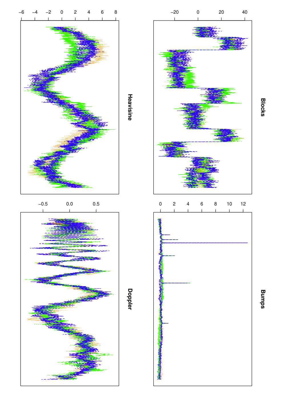
For each mean function associated to a given heteroscedastic structure , the simulation design explores the following configurations: SNR varies in and in . Similarly, the signal and sample size are respectively set to and whereas each configuration is repeated 200 times. Examples of simulated data are represented on Figure 1 for all considered main patterns.
Figure 1 here
Then heteroscedastic thresholding procedures are competed for both Soft and SCAD thresholding functions, and , and for both Universal and SURE threshold, and . Performance of the procedures are evaluated with respect to the Mean Integrated Squared Error (MISE) of the reconstructed mean functions. Simulation results are presented on Figure 2. Examples of reconstruction associated to median performance are represented in Figure 3
Figure 2 and Figure 3 here
As a main conclusion we can observe that using the SURE threshold leads to improved performance for the reconstruction of the main effect in a heteroscedastic setting. As mentionned by Donoho and Johnstone (1995) in the homoscedastic framework, the universal threshold turns out to be too large in practice when dealing with finite dimensional signals.
Another interesting point concerns the interaction between the choice of the threshold and the thresholding function. When using the universal threshold, the SCAD thresholding gives indeed at least similar or improved reconstruction performance. This is expected since the SCAD thresholding is designed to smoothly correct the bias on high coefficients introduced by the soft thresholding. Conversely such a difference vanishes when using the SURE threshold for which Soft and SCAD thresholdings exhibit similar performance. This finding can be explained by the adaptative behaviour of the SURE threshold that compensates the existing bias on high coefficients.
By way of conclusion, the overall simulation study encourages the use of the heteroscedatic thresholding in the context of functional regression with multiple samples. Heteroscedastic thresholding keeps indeed the simplicity and the computational efficiency of the usual homoscedastic thresholding while being able to handle potential inter-individual variations. Moreover, in practice, using the adaptative SURE threshold, paired with the SCAD thresholding which enjoys good theoritical properties leads to improved reconstruction of the mean function.
As a last remark, we shall mention that the wider simulation study abovementioned with various sample and signal sizes shows that the overall MISEs orders of magnitude are more improved by a higher number of samples than by a larger signal size .
4.2 Analysis of experimental data
As an application to the proposed methodology, we analysed a SELDI-TOF mass spectrometry dataset issued from a study on ovarian cancer (Petricoin et al., 2002). This dataset was produced by the Ciphergen WCX2 protein chip and is publicly available through the Clinical Proteomics Programs Databank (11 1 http://home.ccr.cancer.gov/ncifdaproteomics/ppatterns.asp, ovarian dataset 8-7-02). The sample set consists of 162 serums profiles from women affected by an ovarian cancer and 91 control subjects. Each spectra contains the measure of 15154 intensities characterizing as many mass over charge () ratios. Prior to analysis, raw data are background corrected using a quantile regression procedure, and spectra are aligned using a procedure based on wavelets zero crossings (Antoniadis et al., 2007). Moreover, we restrict on 512 intensities for ratios within the range [5200,5915] centered around the main central peak. Mass spectrometry data represented a meaningful application for our method since Giacofci et al. (2013) show evidence for the presence of inter-individual variations occuring at specific ranges of ratios resulting in a sharp heterosecdasticity structure.
We separately analysed the control group and the group affected by a cancer using an heteroscedastic SCAD thresholding procedure, with a SURE threshold. Mean reconstructed functions superimposed on experimental data are represented in Figure 4.
Figure 4 here
We can observe that individuals from the control and cancer groups exhibit similar mean functional profiles. Such an observation indicates that a nonparametric testing procedure would be on purpose to ascertain the presence of a significant effect of the group. Although it is out of the scope of the present paper, in this context, taking into account the presence of potential inter-individual variations appears as critical for the application of such testing procedure.
Acknowledgements
Part of this work was supported by the Interuniversity Attraction Pole (IAP) research network in Statistics P5/24. We are grateful to Anatoli Juditsky for constructive and fruitful discussions.
References
- Amato and Sapatinas (2005) Amato, U. and T. Sapatinas (2005). Wavelet shrinkage approaches to baseline signal estimation from repeated noisy measurements. Advances and Applications in Statistics 51, 21–50.
- Antoniadis et al. (2007) Antoniadis, A., J. Bigot, S. Lambert-Lacroix, and F. Letue (2007). Non parametric pre-processing methods and inference tools for analyzing time-of-flight mass spectrometry data. Current Analytical Chemistry 3(2), 127–147.
- Antoniadis and Fan (2001) Antoniadis, A. and J. Fan (2001). Regularization of wavelet approximations. Journal of the American Statistical Association 96(455), 939–955.
- Antoniadis and Lavergne (1995) Antoniadis, A. and C. Lavergne (1995). Variance function estimation in regression by wavelet methods. Lecture Notes in Statistics ”Wavelets and Statistics” 103, 31–42.
- Antoniadis and Sapatinas (2007) Antoniadis, A. and T. Sapatinas (2007). Estimation and inference in functional mixed-effects models. Computational Statistics & Data Analysis 51(10), 4793–4813.
- Cai and Wang (2008) Cai, T. and L. Wang (2008). Adaptative variance function estimation in heteroscedastic nonparametric regression. The Annals of Statistics 36(5), 2025–2054.
- Coifman and Donoho (1995) Coifman, R. and D. Donoho (1995). Translation invariant de-noising. Wavelets and statistics 103, 125–150.
- Delyon and Juditsky (1997) Delyon, B. and A. Juditsky (1997). On the computation of wavelet coefficients. J. Approximation Theory 88(1), 47–79.
- DeVore and Lorentz (1993) DeVore, R. and G. Lorentz (1993). Constructive approximation. Springer Verlag.
- Donoho (1994) Donoho, D. (1994). Smooth wavelet decompositions with blocky coefficient kernels. L. Schumaker, ed., ‘Recent advances in wavelet analysis’.
- Donoho and Johnstone (1994) Donoho, D. and I. Johnstone (1994). Ideal spatial adaptation by wavelet shrinkage. Biometrika 81(3), 425–455.
- Donoho and Johnstone (1995) Donoho, D. and I. Johnstone (1995). Adapting to unknown smoothness via wavelet shrinkage. Journal of the American Statistical Association 90, 1200–1224.
- Donoho et al. (1995) Donoho, D., I. Johnstone, G. Kerkyacharian, and D. Picard (1995). Wavelet shrinkage: asymptopia. Journal of the Royal Statistical Society, Ser. B 57(2), 371–394.
- Eckel-Passow et al. (2009) Eckel-Passow, J. E., A. L. Oberg, T. M. Therneau, and H. R. Bergen (2009, Jul). An insight into high-resolution mass-spectrometry data. Biostatistics 10, 481–500.
- Fan and Li (2001) Fan, J. and R. Li (2001). Variable selection via nonconcave penalized likelihood and its oracle properties. Journal of the American Statistical Association 96(456), 1348–1360.
- Frazier et al. (1991) Frazier, M., B. Jawerth, and G. Weiss (1991). Littlewood-Paley Theory and the Study of function Spaces. Number 79. American Mathematical Society.
- Gasser et al. (1989) Gasser, T., L. Stroka, and C. Jennen-Steinmetz (1989). Residual variance and residual pattern in nonlinear regression. Biometrika 73, 625–633.
- Giacofci et al. (2013) Giacofci, M., S. Lambert-Lacroix, G. Marot, and F. Picard (2013). Wavelet-based clustering for mixed-effects functional models in high dimension. Biometrics 69(1), 31–40.
- Härdle et al. (1998) Härdle, W., G. Kerkyacharian, D. Picard, and A. Tsybakov (1998). Wavelets, Approximation and Statistical Applications. Springer.
- Johnstone and Silverman (1997) Johnstone, I. and B. Silverman (1997). Wavelet threshold estimators for data with correlated noise. Journal of the Royal Statistical Society, Ser. B 59(2), 319–351.
- Juditsky and Delyon (1996) Juditsky, A. and B. Delyon (1996). On minimax wavelets estimators. Applied and computational harmonic analysis 3, 215–228.
- Mallat (1989) Mallat, S. (1989). Multiresolution approximations and wavelet orthonormal bases of l2(r). Transactions of the American Mathematical Society 315(1), 69–87.
- Morris et al. (2008) Morris, J. S., P. J. Brown, R. C. Herrick, K. A. Baggerly, and K. R. Coombes (2008, Jun). Bayesian analysis of mass spectrometry proteomic data using wavelet-based functional mixed models. Biometrics 64, 479–489.
- Morris and Carroll (2006) Morris, J. S. and R. J. Carroll (2006). Wavelet-based functional mixed models. Journal of the Royal Statistical Society Series B Stat Methodol 68, 179–199.
- Nason (2008) Nason, G. (2008). Wavelet methods in Statistics with R. Springer, New York.
- Park (2010) Park, C. (2010). Block thresholding wavelet regression using {SCAD} penalty. Journal of Statistical Planning and Inference 140(9), 2755 – 2770.
- Petricoin et al. (2002) Petricoin, E. F., A. M. Ardekani, B. A. Hitt, P. J. Levine, V. A. Fusaro, S. M. Steinberg, G. B. Mills, C. Simone, D. A. Fishman, E. C. Kohn, and L. A. Liotta (2002, Feb). Use of proteomic patterns in serum to identify ovarian cancer. Lancet 359, 572–577.
- Stein (1981) Stein, C. (1981). Estimation of the mean of a multivariate normal distribution. The Annals of Statistics 9(6), 1135–1151.
- von Sachs and MacGibbon (2000) von Sachs, R. and B. MacGibbon (2000). Nonparametric curve estimation by wavelet thresholding with locally stationary errors. Scandinavian Journal of Statistics 27(3), 475–499.
5 Appendix
5.1 Proof of Theorem 2.1
First let us recall the aim of the proof concerning the lower bound in the minimax context. Since
for some we have to show that
for some constant . Next we reduce the class to a subclass of finite number of functions in because the is greater over a larger class. The family is constructed by small perturbation of , so that the distance between each pairs of functions is small and at least of order Then the problem can be reduced to the one of testing by the following way
with the power function associated to , where is any test that allows to distinguishing between the hypotheses, the -th of them stating that the observations of model (1) are drawn from the -th element of the set . To bound by we need to major the maximum of the Kullback distance between observations of model (1) associated with and the ones associated with . For instance when we have
Without loss of generality, since variances are assumed to be bounded, we can consider model (1) with , independent and identically distributed Gaussian random variables with zero-mean and variance In this case, we have
| (14) |
Let us come back to the proof of the lower bound. This proof can be decomposed in two steps. For the usual term in we just have to use the usual proof for the Besov classes by adding the factor because of the multiplicative term in (14). We now give the proof corresponding to the term in We only need two functions in order to construct that is For we put for all and
where with support equal to such that and . We have and
So we also have and
hence, the family is inclued in the Besov class and the -distance between the two functions are at at least Since
we have
and
for any estimator
For we use the same method but by choosing
So we have
and
which concludes the proof.
5.2 Proof of Theorem 2.2
This proof is an adaptation of the proof of Theorem 1 of Juditsky and Delyon (1996). We denote by , the estimator with instead of in(6) and the associated estimator. We introduce
where is such that Let us note that (see proposition 1 of Delyon and Juditsky (1997)), there exists some constant such that this function belongs to The global quadratic risk can then be decomposed such that:
| (15) | ||||
We seek to bound from above each term of the decomposition. By using the delta method based on a Taylor expansion of the thresholding function and since are -consistent estimates of variances, we get:
with being a positive constant. The model (2) leads to
Approximation coefficients in are left unchanged, hence we have:
In the same way, terms in are not thresholded, hence we get:
with being a positive constant. The term is the approximation term that can be bounded such that (see proposition 1 of Delyon and Juditsky (1997)):
Finally, bounding term needs the use of constraint (7) with , we have
| (16) |
where For the term , since , we obtain:
For , we have with Cauchy-Schwartz and exponential inequalities:
In order to fix the parameter , the terms and need to be balance according to , which leads to:
By replacing in terms and , the inequality (15) becomes:
The convergence of the overall expression is limited by the terms in and in
The latter leads to a limitation in
Hence, we get:
that concludes the proof.
5.3 Derivation of the SURE criterion for SCAD thresholding
For recall, the SCAD thresholding function is given by:
| (17) |
and we are looking for a function such that:
| (18) |
to define the SURE-SCAD criterion:
| (19) |
with . By defining as the weakly differentiable function:
with , the relation (18) is satisfied. We can then compute:


| SNR | SNR | |||||||
| Ho | He | Ho | He | Ho | He | Ho | He | |
| Blocks | 5.093 | 0.168 | 0.424 | 0.166 | 0.186 | 0.001 | 0.011 | 0.001 |
| (1.629) | (0.018) | (0.130) | (0.017) | (0.054) | (2e-4) | (0.006) | (2e-4) | |
| Bumps | 5.028 | 0.724 | 0.944 | 0.720 | 0.220 | 0.040 | 0.0573 | 0.040 |
| (0.745) | (0.025) | (0.048) | (0.027) | (0.029) | (0.001) | (0.002) | (0.001) | |
| Heavisine | 5.293 | 1.193 | 1.773 | 1.192 | 0.530 | 0.079 | 0.129 | 0.079 |
| () | (0.303) | (0.103) | (0.120) | (0.104) | (0.016) | (0.006) | (0.008) | (0.006) |
| Doppler | 26.79 | 5.607 | 7.819 | 5.629 | 1.387 | 0.187 | 0.304 | 0.188 |
| () | (4.058) | (2.607) | (0.320) | (0.238) | (0.136) | (0.117) | (0.015) | (0.010) |
| SNR | SNR | |||
| Homoscedastic | Heteroscedastic | Homoscedastic | Heteroscedastic | |
| Blocks | 0.189 | 0.168 | 1.44e-3 | 1.43e-3 |
| (0.016) | (0.017) | (2.5e-4) | (2.5e-4) | |
| Bumps | 0.736 | 0.726 | 0.045 | 0.040 |
| (0.024) | (0.024) | (1.25e-3) | (1.25e-3) | |
| Heavisine | 1.203 | 1.204 | 0.079 | 0.078 |
| () | (0.097) | (0.104) | (0.006) | (0.006) |
| Doppler | 5.658 | 5.622 | 0.201 | 0.188 |
| () | (0.246) | (0.274) | (0.011) | (0.011) |