Consensus Driven by the Geometric Mean

Consider data points $x_{1},x_{2},\ldots,x_{n}$ taking values on the positive real line $\mathbb{R}_{>0}$, and let these elements be collected in the vector ${\boldsymbol{x}}$. An average or mean computed from ${\boldsymbol{x}}$ can be obtained as the solution of an unconstrained minimization,

where $d(a,b)$ denotes a metric in $\mathbb{R}_{>0}$, i.e., a positive definite and symmetric function, that vanishes iff $a=b$.

If the Euclidean distance $d_{\mathsf{E}}(a,b):=|a-b|$ is chosen in (1), the resulting average is the arithmetic mean,

Another important metric in $\mathbb{R}_{>0}$ is the hyperbolic distance $d_{\mathsf{H}}(a,b):=|\ln a-\ln b|$, which coincides with the Euclidean metric assessed in logarithmic coordinates. It is a geodesic distance, and measures the hyperbolic length of the straight line segment joining two points in Cartesian coordinates $(x,a),(x,b)$, $x\in\mathbb{R}_{>0}$, see e.g., [27] Prop. 4.3.

Its significance arises from the fact that the solution of the minimization problem (1) using the hyperbolic metric $d_{\mathsf{H}}$ yields the geometric mean

To see this, observe that

which is the least-squares characterization of the arithmetic mean in logarithmic coordinates.

To complete this section we introduce the weighted versions of the arithmetic and geometric means,

where for $i=1,2,\ldots,n$, $\omega_{i}>0$ and $\sum_{i=1}^{n}\omega_{i}=1$.

Let $\mathsf{G}=(N,B,w)$ be a weighted digraph (directed graph) with set of nodes $N:=\{1,2,\ldots,n\}$, set of branches $B:=\{1,2,\ldots,b\}\subseteq N\times N$ having elements ordered pairs $(j,i)$ that indicate that there is a branch from node $j$ to $i$, and $w:B\to\mathbb{R}_{>0}$ is a weighting function for which we write $w((j,i))=w_{ij}$. Define the in-neighborhood of a node $i$ as the set of connected nodes $N_{i}^{+}:=\{j\in N:(j,i)\in B\}$ and the out-neighborhood $N_{i}^{-}:=\{j\in N,(i,j)\in B\}$. The (in-)degree of a node $i$ is the value $d_{i}:=\sum_{j\in N_{i}^{+}}w_{ij}$. Set $\textbf{D}:=\mathsf{diag}\{d_{1},d_{2},\ldots,d_{n}\}$. The weighted adjacency matrix W is such that $[\textbf{W}]_{ij}=w_{ij}$ for all $(j,i)\in B$; if $(j,i)\not\in B$, then $[\textbf{W}]_{ij}=0$, and $[\textbf{W}]_{ii}=0$, for all $i\in N$. A graph is called balanced if $\sum_{j=1}^{n}w_{ij}=\sum_{j=1}^{n}w_{ji}$ and it is symmetric if $w_{ij}=w_{ji}$, $\forall(j,i)\in B$. The Laplacian matrix of a weighted digraph is defined as $\textbf{L}:=\textbf{D}-\textbf{W}$, and the normalized Laplacian is $\hat{\textbf{L}}:=\textbf{I}-\hat{\textbf{W}}$, where $\hat{\textbf{W}}=\textbf{D}^{-1}\textbf{W}$ is the matrix of normalized branch weights.

A linear consensus system evolving in continuous time is a dynamics on a family of graphs $\{\mathsf{G}(t)\}_{t\geq 0}$ governed by

where each dynamic branch weight $w_{ij}(\cdot)$ is a measurable non-negative function [28].

The following relationships between the arithmetic mean and consensus system representations and properties are well known in consensus theory: Using (2), a component-wise LTI consensus dynamics (6) on a normalized weighted digraph can locally be brought to the open-loop control system form

Without the requirement of a normalized weighting, a variable time discretization can be chosen such that a local algorithmic update law (e.g. in an explicit Euler scheme) has the arithmetic mean driven form

where $0\leq\alpha<1$, cf., e.g., [10].

Besides its appearance in the local dynamics at a certain instant in time, the arithmetic average unfolds also as asymptotic global system property: in the class of consensus networks being governed by Laplacians $\textbf{L}(t)$ that are irreducible and balanced for all $t\geq 0$, the asymptotically reached uniform agreement value is given by the arithmetic mean of the initial condition [29]. The problem in which the equilibrium state to be reached is uniform with consensus value $\bar{x}=\mathsf{am}({\boldsymbol{x}}_{0})$ is commonly known as the average consensus problem.

The goal in this work is to study the interplay between consensus protocols and the geometric mean. In that, we first seek to understand the various interaction points between the design of LTI consensus protocols and the arithmetic mean, and then leverage these observations to derive and study novel geometric mean driven consensus protocols.

For the sake of focus and ease of understanding, we assume the underlying graph to have a constant, i.e., time-invariant weighting. In our analysis it shall turn out elementary to transform the non-linear time-invariant network protocols to linear time-varying consensus form, so that the following convergence result becomes applicable.

Uniform connectivity certainly holds if at each time instant the graph $\mathsf{G}(t)$ is strongly connected and $w_{ij}(t)\geq\delta>0$, i.e., if the graph contains a directed path from every node to every other node and the finite branch weights are positively bounded away from zero for all time.

The polynomial protocol we consider is a dynamics on a graph where at each node $i\in N$, the differential update rule has the form

For the polynomial protocol we assume a balanced graph weighting, i.e., $\sum_{j\in N_{i}^{-}}w_{ji}=d_{i}$. With that, the protocol (11) can be written as

Comparing this form with a linear consensus protocol, which can be stated as

we observe an equivalence resulting upon replacing the operation of summation and multiplication with the similar¹¹ 1 These operations are similar in the sense that the addition of logarithmic variables turns the variables into products, and products result into exponentiation. operations multiplication and exponentiation.

Alternatively, referring to the open-loop control representation (7), where weightings are normalized, replacement of the weighted arithmetic mean by the geometric average leads to the protocol

from where (11) results again under the assumption of having a balanced weighting, that is, $\sum_{j\in N_{i}^{-}}\hat{w}_{ji}=1$.

In its general form (11), the polynomial protocol has the structure of a rate equation as it occurs for instance in reaction networks and chemical kinetics [16]. We define

the non-linear rate at which some quantity “$x$” flows from in-connected nodes $j$ to node $i$, and

the rate at which $x$ flows along links $(i,j)\in B$ from node $i$ to the out-directed nodes $j$. The local rate of change $\dot{x}_{i}$ balances in- and out-flows on a graph, as $\dot{x}_{i}=r_{i}^{+}({\boldsymbol{x}})-r_{i}^{-}({\boldsymbol{x}})$. The relation to the (weighted) geometric mean and the similarity to chemical kinetics in reaction networks are described in the following example.

The entropic protocol is governed by a vector field that is represented by a set of negative (weighted) divergences between local states $x_{i}$ and connected nodes’ states $x_{j}$, such that

The term “entropic” refers to the fact that a local vector field (20) is an entropic quantity. More precisely, it has the structure of a negative relative entropy / information divergence between the local state $x_{i}$ and the adjacent states $x_{j}$, $j\in N_{i}^{+}$. Relative entropy as divergence from a positive vector ${\boldsymbol{x}}$ to another positive vector ${\boldsymbol{y}}$, both such that their $1$-norms equal one, (i.e., these are probability mass vectors), is defined as

see for instance  [33].

The entropic protocol can be formulated as the geometric mean version of the linear consensus protocol using a coordinate transformation, with coordinate transform taken as the scalar function that leads to a least squares variational characterization of the considered mean; for the geometric mean this is the logarithm, while for the arithmetic mean no coordinate transformation is required, see (2) with (4).

Writing the consensus protocol in logarithmic coordinates leads for each $i\in N$ to the ODE

which is the entropic protocol (20), as

As we shall show, the significance of the entropic protocol arises from the situation that the asymptotically reached consensus value is given by the geometric mean of the initial condition. Hence, this protocol provides an analog distributed computation routine to solve the minimization (1) associated to the geometric mean.

In this section, we introduce the scaling-invariant protocol as an instance of a novel class of network dynamics driven by pairwise metric interactions.

The scaling-invariant protocol has the form of a LTI consensus system however following log-linear updates; it is given by the component ODE

This is an instance of the more general type of mean-driven network protocols given by the class

where the metric to be chosen is the hyperbolic metric $d_{\mathsf{H}}$ associated to the variational characterization of the geometric mean, see section II.

The general mean-driven equation (26) can be motivated from a system thermodynamic viewpoint; in [34] a network protocol is proposed with pairwise interactions of the form $f(x_{i},x_{j})$, where $f$ is locally Lipschitz continuous and assumed to satisfy the condition $(x_{i}-x_{j})f(x_{i},x_{j})\leq 0$, $f(x_{i},x_{j})=0$ if $x_{i}=x_{j}$. According to the authors this assumption implies that some sort of energy or information flows from higher to lower levels thus this condition is reminiscent of a “second law”-like inequality in thermodynamics.

We observe that this negativity hypothesis is naturally fulfilled by a metric interaction form as in (26): for any two states the sign of the terms $(x_{i}-x_{j})$ and $f(x_{i},x_{j})$ must differ. Hence, for two arguments $x_{i},x_{j}$, $f$ has the sign $\mathsf{sign}(x_{j}-x_{i})$. Therefore, we get the structure $f=\mathsf{sign}(x_{j}-x_{i})f_{\mathrm{res}}$ with residual part required to be positive definite. The choice $f_{\mathrm{res}}=d$ follows naturally.

To study stability of fixed-points we shall make use of the logarithmic mean, its properties and the mean value theorem: The logarithmic mean of two positive real numbers $a,b$ is defined as

The logarithmic mean is positive and symmetric in both arguments, i.e., $\mathsf{lgm}(a,b)=\mathsf{lgm}(b,a)$. The mean value theorem states that for a continuously differentiable function $f:[a,b]\subseteq\mathbb{R}\to\mathbb{R}$, there exists a $\xi\in[a,b]$ such that

With $f=\ln$, we get $\mathsf{lgm}(a,b)=\xi$, where $0<a\leq\xi\leq b$.

The logarithmic mean and its inverse take positive and finite values for positive and finite arguments. For approaching positive real arguments we further have

so that $\lim_{b\to a}\mathsf{lgm}(a,b)=a>0$.

This proof technique is of interest in its own right: we make use of the Laplacian structure arising from (algebraic) interconnections on a graph in shifting non-linearity associated to nodes to a non-linearity in pairwise interactions across branches, leading to a “virtual” dynamic graph on which the non-linear time-invariant network dynamics appears as linear time-varying consensus system.

In the following result we analytically characterize the consensus value of the entropic consensus network.

Regarding the asymptotically reached agreement value of the polynomial consensus protocol the maximum and minimum initial state values provide upper and lower bounds by standard linear consensus theory. So far we could not analytically derive tighter results. However, comprehensive numerical simulations, see appendix, suggest that the consensus value is upper bounded by the arithmetic mean of the initial condition and lower bounded by the arithmetic geometric mean of the arithmetic mean and the geometric mean of the initial state. This value is related to the solution of an elliptic integral. The proof of this conjecture is subject to future work. For further information we refer the interested reader to the appendix and references stated therein.

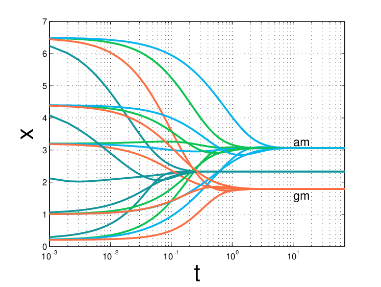
First, we compare the protocols of polynomial type (28), of entropic type (29) and the scaling-invariant one (30) for a digraph given in Fig. 2(a). This digraph is strongly connected and has balanced branch weights.

For each of these protocols we compute trajectories starting at ${\boldsymbol{x}}(0)=[6.5,0.2,3.2,1,4.4]$. In accordance to Theorem 1, the novel network protocols are indeed consensus protocols that converge to a uniform equilibrium state $\bar{x}{\boldsymbol{1}}$. As the left-Perron vector for the balanced weighting is a uniform vector, the LTI consensus system must solve the average consensus problem with $\bar{x}=\mathsf{am}({\boldsymbol{x}}(0))=3.06$, the scaling-invariant protocol, according to Corollary 1, as well, and solution curves of the entropic protocol must converge to the geometric mean of the initial state, $\mathsf{gm}({\boldsymbol{x}}(0))=1.7886=\bar{x}$, as shown in Theorem 2. Our observations are confirmed by Fig. 2(c).

Next, let us illustrate the results in Theorem 2 and Corollary 1 on a digraph which is strongly connected but not balanced. We consider a weighted digraph described in Fig. 2(b), which has Perron vector $\hat{{\boldsymbol{q}}}=[0.26,0.14,0.37,0.09,0.14]$. The weighted arithmetic mean of the same initial condition using the Perron vector components as weights is $\mathsf{am}_{w}({\boldsymbol{x}}(0))=3.5884$, and the weighted geometric mean becomes $\mathsf{gm}_{w}({\boldsymbol{x}}(0))=2.4444$. Again, the simulation results as depicted in Fig. 2(d) confirm our observations.

Free energy stored in a state ${\boldsymbol{x}}$ w.r.t. another positive vector ${\boldsymbol{y}}$ can be defined as the sum-separable function [30]

For elements that are member of the set of vectors having total mass $m\in\mathbb{R}_{>0}$,

free energy is, up to an additive constant, a relative entropy; it coincides with the usual relative entropy known in information theory for vectors that are elements of the set of probability distribution vectors, $\mathscr{D}_{m=1}$, by setting $const=1$, so that $F({\boldsymbol{x}}||{\boldsymbol{y}})=\sum_{i=1}^{n}x_{i}\ln\frac{x_{i}}{y_{i}}$.

In what follows we show that the polynomial, entropic, and scaling-invariant consensus dynamics are all instances of a particular type of a free energy gradient flow.

To start with, an ODE governing a Riemannian gradient (descent) flow in $\mathbb{R}^{n}$ has the generic form $\textbf{G}({\boldsymbol{x}})\dot{{\boldsymbol{x}}}=-\nabla E({\boldsymbol{x}})$ where $E:\mathbb{R}^{n}\to\mathbb{R}$ is the potential and $\textbf{G}:\mathbb{R}^{n}\to\mathbb{R}^{n\times n}$ is a positive definite matrix function smoothly varying in ${\boldsymbol{x}}$. It defines the infinitesimal metric $\mathrm{d}{\boldsymbol{x}}\cdot\textbf{G}({\boldsymbol{x}})\mathrm{d}{\boldsymbol{x}}$ in which a system is a gradient descent flow of $E$, so that $\textbf{G}^{-1}$ defines the inverse metric, cf., e.g., [38].

Let L be the symmetric Laplacian of an undirected connected graph. Using the eigen-decomposition $\textbf{L}=\textbf{V}{\boldsymbol{\Lambda}}\textbf{V}^{\top}$, where ${\boldsymbol{\Lambda}}:=\mathsf{diag}\{\lambda_{1},\lambda_{2},\ldots,\lambda_{n}\}$ is the diagonal matrix collecting eigenvalues of L, and V collects orthogonal eigenvectors each having 2-norm one, we have

which is a projection of a vector ${\boldsymbol{x}}$ onto the set of distributions $\mathscr{D}_{m},m=|{\boldsymbol{x}}|_{1}$. To see this, recall that a projection onto this set has the form

where $\{\tilde{{\boldsymbol{v}}}_{1},\tilde{{\boldsymbol{v}}}_{2},\ldots,\tilde{{\boldsymbol{v}}}_{n-1}\}$ are linearly independent vectors that span the hyperplane $\mathscr{D}_{m}$. This setting is given in (52), as $\lambda_{1}=0$, while $\lambda_{i}>0,i=2,3,\ldots,n$, and ${\boldsymbol{v}}_{1}$ is orthogonal to any set $\mathscr{D}_{m}$.

Given a sum-separable convex function $\phi:\mathbb{R}^{n}_{>0}\to\mathbb{R}$ we introduce for the gradient $\nabla\phi$ projected onto $\mathscr{D}_{m},m=|\nabla\phi|_{1}$, the notation $\nabla_{\mathscr{D}}\phi=\textbf{L}\nabla\phi$. Observe that the gradient $\nabla F({\boldsymbol{x}}||{\boldsymbol{1}})$ is given by the vector $\ln{\boldsymbol{x}}$. Using the projected gradient notation, we can write the protocols (28)-(30) in same order in vector matrix form as

with L the constant coefficient Laplacian, and $\textbf{R}({\boldsymbol{x}}),\textbf{X}({\boldsymbol{x}})$ as in the proof of Theorem 1. As $\textbf{R}({\boldsymbol{x}})$ and $\textbf{X}({\boldsymbol{x}})$ are positive definite symmetric matrix functions for ${\boldsymbol{x}}\in\mathbb{R}_{>0}^{n}$, they define Riemannian metrics via their inverses.

The scaling-invariant protocol on an undirected graph generates a projected gradient flow in the usual Euclidean metric setting. Therefore, according to the preceding discussion, on a completely normalized graph trajectories must evolve along steepest descent directions of free energy on the appropriate simplex of constant mass distributions.

In Fig. 3 this free energy gradient property is illustrated for the scaling-invariant protocol running on such a graph over three nodes. The gray outlined triangle marks the set of mass-3 distribution vectors. Color-coded are iso-level curves of $F({\boldsymbol{x}}||{\boldsymbol{1}})=\sum_{i}x_{i}(\ln x_{i}-1)+3$. This illustration also highlights the appropriateness of the $n-1$-dimensional set of mass distribution vectors within positive $n$-space in considering the free energy functional: Free energy is convex and permutation invariant on this set with minimum obtained at the consensus state. Three trajectories are plotted in black with initial conditions marked by a cross. We see that solution curves indeed follow steepest gradient descent directions of free energy on $\mathscr{D}_{m=3}$ being directed towards the minimum of this function, which is obtained at the consensus point.

Motivated by the preceding results for the entropic protocol we provide a novel variational characterization of the geometric mean linking dynamic problems in consensus theory with static problems in non-linear constrained optimization.

Sum-separable energy functions play an axiomatic role in dissipative interconnected systems [39] where they represent energy stored in local subsystems. In contrast, energy functions of the interaction type usually represent power dissipated “across”, e.g., resistor elements, see for instance [40] for a further discussion. Hence, the free energy minimization property seems to be the natural gradient setting for the time-continuous entropic consensus network when seen as analog circuit device solving a minimization problem.

References

- [1] R. Olfati-Saber, J. Fax, and R. Murray, “Consensus and cooperation in networked multi-agent systems,” Proceedings of the IEEE, vol. 95, pp. 215–233, Jan 2007.
- [2] D. P. Bertsekas and J. Tsitsiklis, Parallel and Distributed Computation: Numerical Methods. Prentice-Hall, 1989.
- [3] L. Moreau, “Stability of continuous-time distributed consensus algorithms,” in 43rd IEEE Conference on Decision and Control, pp. 3998–4003, 2004.
- [4] J. A. Acebrón, L. L. Bonilla, C. J. P. Vicente, F. Ritort, and R. Spigler, “The Kuramoto model: A simple paradigm for synchronization phenomena,” Reviews of Modern Physics, vol. 77, no. 1, pp. 137–185, 2005.
- [5] F. Dörfler and F. Bullo, “Synchronization in complex networks of phase oscillators: A survey,” Automatica, vol. 50, pp. 1539–1564, 2014.
- [6] F. Dörfler and J. M. Hendrickx, “Synchronization of oscillators: Feasibility and non-local analysis,” in LCCC Workshop on Dynamics and Control in Networks http://www.lccc.lth.se/index.php?page=open-problems, 2014.
- [7] M. Breakspear, S. Heitmann, and A. Daffertshofer, “Generative models of cortical oscillations: from Kuramoto to the nonlinear Fokker Planck equation,” Frontiers in Human Neuroscience, vol. 4, no. 190, p. 10.3389/fnhum.2010.00190, 2010.
- [8] R. Sepulchre, “Consensus on nonlinear space,” Annual reviews in control, vol. 35, no. 1, pp. 56–64, 2011.
- [9] A. Sarlette and R. Sepulchre, “Consensus optimization on manifolds,” SIAM Journal on Control and Optimization, vol. 48, pp. 56–76, 2009.
- [10] L. Scardovi, A. Sarlette, and R. Sepulchre, “Synchronization and balancing on the n-torus,” Systems & Control Letters, vol. 56, no. 5, pp. 335–341, 2007.
- [11] A. Jadbabaie, N. Motee, and M. Barahona, “On the stability of the Kuramoto model of coupled nonlinear oscillators,” in American Control Conference, 2004. Proceedings of the 2004, vol. 5, pp. 4296–4301 vol.5, June 2004.
- [12] L. Spizman and M. A. Weinstein, “A note on utilizing the geometric mean: when, why and how the forensic economist should employ the geometric mean,” Journal of Legal Economics, vol. 15, pp. 43–55, 2008.
- [13] M. Zenner, S. Hill, J. Clark, and N. Mago, “The most important number in finance - the quest for the market risk premium,” tech. rep., JP Morgan, 2008.
- [14] D. W. Mitchell, “More on spreads and non-arithmetic means,” The Mathematical Gazette, vol. 88, no. 511, pp. 142–144, 2004.
- [15] A. Shingleton, “Allometry: The study of biological scaling,” Nature Education Knowledge, vol. 3, no. 10, p. 2, 2010.
- [16] K. A. Connors, Chemical Kinetics - The Study of Reaction Rates in Solution. VCH Publishers, Inc., 1990.
- [17] Y. Hori, T.-H. Kim, and S. Hara, “Existence criteria of periodic oscillations in cyclic genere regulatory networks,” Automatica, vol. 47, pp. 1203–1209, 2011.
- [18] S. Bandyopadhyay and S.-J. Chung, “Distributed estimation using Bayesian consensus filtering,” in IEEE American Control Conference (ACC), pp. 634–641, 2014.
- [19] L. Qipeng, Z. Jiuhua, and W. Xiaofan, “Distributed detection via Bayesian updates and consensus,” in 34th Chinese Control Conference (CCC), pp. 6992–6997, 2015.
- [20] C. Genest and J. V. Zidek, “Combining probability distributions: A critique and an annotated bibliography,” Statistical Science, vol. 1, no. 1, pp. 114–148, 1986.
- [21] A. Nedić, A. Olshevsky, and C. A. Uribe, “Fast convergence rates for distributed non-Bayesian learning,” arXiv:1508.05161v1 [math.OC], 2015.
- [22] S. Shahrampour and A. Jadbabaie, “Exponentially fast parameter estimation in networks using distributed dual averaging,” in 52nd IEEE Conference on Decision and Control, pp. 6196–6201, 2013.
- [23] M. A. Rahimian and A. Jadbabaie, “Learning without recall: A case of log-linear learning,” IFAC-PapersOnLine, vol. 48, no. 22, pp. 46–51, 2015.
- [24] R. Hegselmann and U. Krause, “Opinion dynamics driven by various ways of averaging,” Computational Economics, vol. 25, pp. 381–405, 2005.
- [25] I. Matai and J. S. Baras, “The asymptotic consensus problem on convex metric spaces,” IEEE Transactions on Automatic Control, vol. 60, no. 4, pp. 907 – 921, 2015.
- [26] A. Bishop and A. Doucet, “Distributed nonlinear consensus in the space of probability measures,” in Proceedings of the 19th IFAC World Congress, 2014.
- [27] S. Stahl, The Poincaré Half-Plane - A Gateway to Modern Geometry. Jones and Bartlett Publishers, 1993.
- [28] J. M. Hendrickx and J. N. Tsitsiklis, “Convergence of type-symmetric and cut-balanced consensus seeking systems,” IEEE Transaction on Automatic Control, vol. 58, pp. 214–218, 2013.
- [29] R. Olfati-Saber and R. M. Murray, “Consensus problems in networks of agents with switching topology and time-delays,” IEEE Transactions on Automatic Control, vol. 49, p. 9, 2004.
- [30] A. van der Schaft, S. Rao, and B. Jayawardhana, “On the mathematical structure of balanced chemical reaction networks governed by mass action kinetics,” SIAM Journal on Applied Mathematics, vol. 73, no. 2, pp. 953–973, 2013.
- [31] A. van der Schaft, S. Rao, and B. Jayawardhana, “On the network thermodynamics of mass action chemical reaction networks,” in 1st IFAC Workshop on Thermodynamic Foundations of Mathematical Systems Theory, pp. 24–29, 2013.
- [32] W.-A. Yong, “Conservation-dissipation structure of chemical reaction systems,” Physical Review E, vol. 86, p. 067101, 2012.
- [33] T. M. Cover and J. A. Thomas, Elements of Information Theory. John Wiley & Sons, Inc., 1991.
- [34] Q. Hui and W. M. Haddad, “Distributed nonlinear control algorithms for network consensus,” Automatica, vol. 44, pp. 2375–2381, 2008.
- [35] R. Olfati-Saber and R. M. Murray, “Consensus protocols for networks of dynamic agents,” in American Control Conference, pp. 951–956, 2003.
- [36] R. Sepulchre, A. Sarlette, and P. Rouchon, “Consensus in non-commutative spaces,” in Decision and Control (CDC), 2010 49th IEEE Conference on, pp. 6596–6601, Dec 2010.
- [37] L. Moreau, “Stability of multiagent systems with time-dependent communication links,” IEEE Transactions on Automatic Control, vol. 50, pp. 169–182, 2005.
- [38] J. W. Simpson-Porco and F. Bullo, “Contraction theory on Riemannian manifolds,” Systems Control Letters, vol. 65, pp. 74–80, 2014.
- [39] J. C. Willems, “Dissipative dynamical systems part 1: General theory,” Archive for Rational Mechanics and Analysis, vol. 45, pp. 321– 351, 1972.
- [40] H. Mangesius, J.-C. Delvenne, and S. K. Mitter, “Gradient and passive circuit structure in a class of non-linear dynamics on a graph,” Systems and Control Letters, vol. 96, pp. 30– 36, 2016.
- [41] S. Adlaj, “An eloquent formula for the perimeter of an ellipse,” Notices of the AMS, vol. 59, pp. 1094–1099, 2012.
- [42] J. M. Borwein and P. B. Borwein, Pi and the AGM - A Study in Analytic Number Theory and Computational Complexity. John Wiley & Sons, Inc., 1987.
- [43] B. Carlson, “Algorithm involving arithmetic and geometric means,” The American Mathematical Monthly, vol. 78, pp. 496–505, 1971.