跳到论文正文
W Papers独立论文阅读器 arXiv:1511.02452 论文正文 计算阅读时间 · 0%
引用这篇论文根据当前论文元数据生成,正式投稿前建议核对。


License: arXiv.org perpetual non-exclusive license
arXiv:1511.02452v2 [hep-ph] 04 Mar 2016

Octant Degeneracy, Quadrant of CPV phase at Long Baseline ν\nu Experiments and Baryogenesis

Kalpana Bora Affiliation: Department Of Physics, Gauhati University, Guwahati-781014, India    Gayatri Ghosh Affiliation: Department Of Physics, Gauhati University, Guwahati-781014, India    Debajyoti Dutta Affiliation: Harish-Chandra Research Institute, Chhatnag Road, Jhunsi, Allahabad 211019, India
Abstract

In a recent work by two of us, we have studied, how CP violation discovery potential can be improved at long baseline neutrino experiments (LBNE/DUNE), by combining with its ND (near detector) and reactor experiments. In this work, we discuss how this study can be further analysed to resolve entanglement of the quadrant of leptonic CPV phase and Octant of atmospheric mixing angle θ23\theta_{23}, at LBNEs. The study is done for both NH (Normal hierarchy) and IH (Inverted hierarchy), HO (Higher Octant) and LO (Lower Octant). We show how leptogenesis can enhance the effect of resolving this entanglement, and how possible values of the leptonic CPV phase can be predicted in this context. Carrying out numerical analysis based on the recent updated experimental results for neutrino mixing angles, we predict the values of the leptonic CPV phase for 152 possible cases. We also confront our predictions of the leptonic CPV phase with the updated global fit and find that five values of δC​P\delta_{CP} are favoured by BAU constraints. One of the five values matches with the recent global fit value of δC​P\delta_{CP} (leptonic CPV phase) close to 1.41π\pi in our model independent scenario. A detailed analytic and numerical study of baryogenesis through leptogenesis is performed in this framework in a model independent way.

I Introduction

Today, physics is going through precision era-this is more so for Neutrino physics. With the measurement of reactor angle θ13\theta_{13} [1, 2, 3] precisely by reactor experiments, the unknown quantities left to be measured in neutrino sector are −- leptonic CP violating phase [4, 5, 6, 7, 8, 9], octant of atmospheric angle θ23\theta_{23} [10, 11, 12, 13, 14], mass hierarchy, nature of neutrino etc. Long baseline neutrino experiments (LBNE [15, 16], NOν\nuA [17] , T2K [18], MINOS [19], LBNO [20] etc) may be very promising, in measuring many of these sensitive parameters.

Exploring leptonic CP violation (CPV) is one of the most demanding tasks in future neutrino experiments [21]. The relatively large value of the reactor mixing angle θ13\theta_{13} measured with a high precision in neutrino experiments [22] has opened up a wide range of possibilities to examine CP violation in the lepton sector. The leptonic CPV phase can be induced by the PMNS neutrino mixing matrix [23] which holds, in addition to the three mixing angles, a Dirac type CP violating phase in general as it exists in the quark sector, and two extra phases if neutrinos are Majorana particles. Even if we do not yet have significant evidence for leptonic CPV, the current global fit to available neutrino data manifests nontrivial values of the Dirac-type CP phase [24, 25]. In this context, possible size of leptonic CP violation detectable through neutrino oscillations can be predicted. Recently, [4], two of us have explored possibiities of improving CP violation discovery potential of newly planned Long-Baseline Neutrino Experiments (earlier LBNE, now called DUNE) in USA. In neutrino oscillation probability expression P(νμ→νe\nu_{\mu}\rightarrow\nu_{e}) relevant for LBNEs, the term due to significant matter effect, changes sign when oscillation is changed from neutrino to antineutrino mode, or vice-versa. Therefore in presence of matter effects, CPV effect is entangled and hence, one has two degenerate solutions - one due to CPV phase and another due to its entangled value. It has been suggested to resolve this issue by combining two experiments with different baselines [26, 27]. But CPV phase measurements depends on value of reactor angle θ13\theta_{13}, and hence precise measurement of θ13\theta_{13} plays crucial role in its CPV measurements. This fact was utilised recently by two of us [4], where we explored different possibilities of improving CPV sensitivity for LBNE, USA. We did so by considering LBNE with
1. Its ND (near detector).
2. And reactor experiments.

We considered both appearance (νμ→νe\nu_{\mu}\rightarrow\nu_{e}) and disappearance (νμ→νe\nu_{\mu}\rightarrow\nu_{e}) channels in both neutrino and antineutrino modes. Some of the observations made in [4] are
1. CPV discovery potential of LBNE increases significantly when combined with near detector and reactor experiments.
2. CPV violation sensitivity is more in LO (lower octant) of atmospheric angle θ23\theta_{23}, for any assumed true hierarchy.
3. CPV sensitivity increases with mass of FD (far detector).
4. When NH is true hierarchy, adding data from reactors to LBNE improve its CPV sensitivity irrespective of octant.

Aim of this work is to critically analyse the results presented in [4], in context of entanglement of quadrant of CPV phase and octant of θ23\theta_{23}, and hence study the role of leptogenesis (and baryogenesis) in resolving this enganglement. Though in [4], we studied effect of both ND and reactor experiments on CPV sensitivity of the LBNEs, in this work we have considered only the effect of ND. But similar studies can also be done for the effect of Reactor experiments on LBNEs as well. The details of LBNE and ND are same as in [4]. Following the results of [4], either of the two octants is favoured, and the enhancement of CPV sensitivity with respect to its quadrant is utilized here to calculate the values of lepton-antilepton symmetry. This is done considering two cases of the rotation matrix for the fermions - CKM only, and CKM+PMNS. Then, this is used to calculate the value of BAU. This is an era of precision measurements in neutrino physics. We therefore consider variation of Δ​m312\Delta m^{2}_{31} within its 1σ\sigma, 2σ\sigma and 3σ\sigma range values. We calculate baryon to photon ratio, and compare with its experimentally known best fit value. We observe that the BAU can be explained most favourably for five possible cases explored here: IH, δC​P=1.43​π\delta_{CP}=1.43\pi and HO of θ23\theta_{23}; IH, δC​P=0.5277​π\delta_{CP}=0.5277\pi and HO of θ23\theta_{23}; IH, δC​P=0.488​π\delta_{CP}=0.488\pi and LO of θ23\theta_{23}; IH, δC​P=0.383​π\delta_{CP}=0.383\pi and HO of θ23\theta_{23}; IH, δC​P=1.727​π\delta_{CP}=1.727\pi and LO of θ23\theta_{23}. It is worth mentioning that the value of δC​P=1.43​π\delta_{CP}=1.43\pi favoured by our calculation here is close to the central value of δC​P\delta_{CP} from the recent global fit result [25, 28]. We also find that for variation of Δ​m312\Delta m^{2}_{31}, within its 1σ\sigma range, the calculated values of ηB\eta_{B} for all possible five cases mentioned above lie in the allowed range of its best fit value. But for 3 σ\sigma variation of Δ​m312\Delta m^{2}_{31}, some of its values at its 3σ\sigma C.L are disfavoured. Also for the variation of θ13\theta_{13} within its 3 σ\sigma C.L, its values around 9.0974 are favoured, as far as matching with the best fit values of ηB\eta_{B} are concerned. These results could be important keeping in view that the quadrant of leptonic CPV phase, and octant of atmospheric mixing angle θ23\theta_{23} are yet not fixed. Also, they are significant in context of precision measurements on neutrino oscillation parameters.

The paper is organized as follows. In Section II, we discuss entanglement of quadrant of CPV phase and octant of θ23\theta_{23}. In Section III, we present a review on leptogenesis and baryogenesis. In Sec. IV we show how the baryon asymmetry (BAU) within the SO(10) model, by using two distinct forms for the lepton CP asymmetry, can be used to break the entanglement. Sec. V summarizes the work.

II CPV Phase and Octant of θ23\theta_{23}

As discussed above, from Fig. 3 of [4], we find that by combining with ND and reactor experiments, CPV sensitivity of LBNE improves more for LO (lower octant) than HO (higher octant), for any assumed true hierarchy. In Fig. 1 below we plot CP asymmetry,

AC​P=P⁡(νμ→νe)−P⁡(νμ¯→νe¯)P⁡(νμ→νe)+P⁡(νμ¯→νe¯)A_{CP}=\frac{P(\nu_{\mu}\rightarrow\nu_{e})-P(\overline{\nu_{\mu}}\rightarrow\overline{\nu_{e}})}{P(\nu_{\mu}\rightarrow\nu_{e})+P(\overline{\nu_{\mu}}\rightarrow\overline{\nu_{e}})} (1)

as a function of leptonic CPV phase δC​P\delta_{CP}, for 0 ≤δC​P≤2​π\leq\delta_{CP}\leq 2\pi. It was shown in [4] that, using near detector (and combining with reactor experiments) at LBNE, the sentivity to measure CPV phase (and hence CP asymmetry) improves more at lower octant of θ23\theta_{23}. CP asymmetry also depends on the mass hierarchy. For NH, CP asymmetry is more in LO than in HO. For IH, CP asymmetry is more in LO than in HO. In this work we have used above information to calculate dependance of leptogenesis on octant of θ23\theta_{23} and quadrant of CPV phase.

Refer to caption

Figure 1: CP asymmetry vs δC​P\delta_{CP} at DUNE/LBNE, for both the hierarchies. In Fig. 1 red and green solid (dotted) lines are for NH (IH) with types of curve to distinguish HO and LO as the true octant respectively.

From Fig. 1 we see that

AC​P​(L​O)>AC​P​(H​O)A_{CP}(LO)>A_{CP}(HO) (2)

For a given true hierarchy, there are eight degenerate solutions

δC​P​(first quadrant)−θ23​(lower octant)\delta_{CP}(\text{first quadrant})-\theta_{23}(\text{lower octant})
δC​P​(second quadrant)−θ23​(lower octant)\delta_{CP}(\text{second quadrant})-\theta_{23}(\text{lower octant})
δC​P​(third quadrant)−θ23​(lower octant)\delta_{CP}(\text{third quadrant})-\theta_{23}(\text{lower octant})
δC​P​(fourth quadrant)−θ23​(lower octant)\delta_{CP}(\text{fourth quadrant})-\theta_{23}(\text{lower octant})
δC​P​(first quadrant)−θ23​(higher octant)\delta_{CP}(\text{first quadrant})-\theta_{23}(\text{higher octant})
δC​P​(second quadrant)−θ23​(higher octant)\delta_{CP}(\text{second quadrant})-\theta_{23}(\text{higher octant})
δC​P​(third quadrant)−θ23​(higher octant)\delta_{CP}(\text{third quadrant})-\theta_{23}(\text{higher octant})
δC​P​(fourth quadrant)−θ23​(higher octant)\delta_{CP}(\text{fourth quadrant})-\theta_{23}(\text{higher octant}) (3)

This eight-fold degeneracy can be viewed as

Quadrant of CPV phase−Octant of​θ23\text{Quadrant of CPV phase}-\text{Octant of}\hskip 2.84544pt\theta_{23} (4)

entanglement. Out of these eight degenerate solutions, only one should be true solution. To pinpoint one true solution, this entanglement has to be broken. We have shown [4] that sensitivity to discovery potential of CPV at LBNEs in LO is improved more, if data from near detector of LBNEs, or from Reactor experiments is added to data from FD of LBNEs as shown in Fig. 3 of [4]. Therefore 8-fold degeneracy of (3) gets reduced to 4-fold degeneracy, with our proposal [4]. Hence, following this 4-fold degeneracy still remains to be resolved.

δC​P​(first quadrant)−θ23​(LO)\delta_{CP}(\text{first quadrant})-\theta_{23}(\text{LO})
δC​P​(second quadrant)−θ23​(LO)\delta_{CP}(\text{second quadrant})-\theta_{23}(\text{LO})
δC​P​(third quadrant)−θ23​(LO)\delta_{CP}(\text{third quadrant})-\theta_{23}(\text{LO})
δC​P​(fourth quadrant)−θ23​(LO)\delta_{CP}(\text{fourth quadrant})-\theta_{23}(\text{LO}) (5)

The possibility of θ23>450\theta_{23}>45^{0}, ie HO of θ23\theta_{23} is also considered in this work. In this context the degeneracy is

δC​P​(first quadrant)−θ23​(HO)\delta_{CP}(\text{first quadrant})-\theta_{23}(\text{HO})
δC​P​(second quadrant)−θ23​(HO)\delta_{CP}(\text{second quadrant})-\theta_{23}(\text{HO})
δC​P​(third quadrant)−θ23​(HO)\delta_{CP}(\text{third quadrant})-\theta_{23}(\text{HO})
δC​P​(fourth quadrant)−θ23​(HO)\delta_{CP}(\text{fourth quadrant})-\theta_{23}(\text{HO}) (6)

Refer to caption
Refer to caption
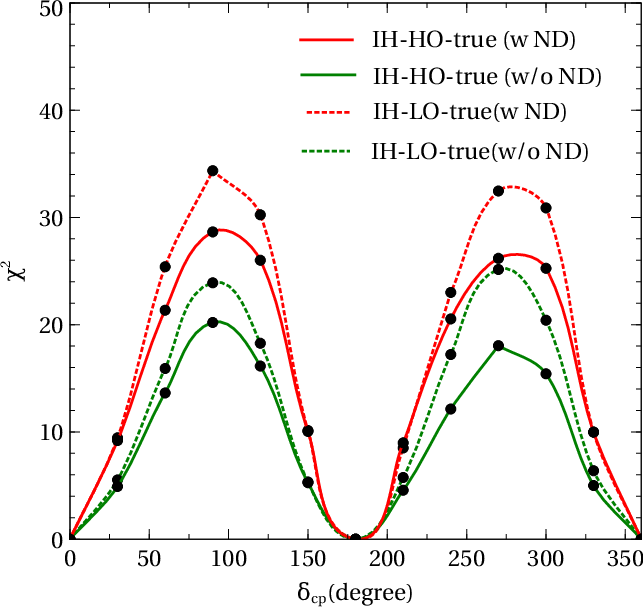
Figure 2: In Fig. 2a and 2b δC​P\delta_{CP} Vs Δ​χ2\Delta\chi^{2} sensitivity corresponding to CP discovery potential at LBNEs, for both the hierarchies and octant is shown.

In this work, we propose that leptogenesis can be used to break above mentioned 4-fold degeneracy of Eq. (5),(6). It is known that observed baryon asymmetry of the Universe (BAU) can be explained via leptogenesis [29, 30, 31, 32, 33]. In leptogenesis, the lepton-antilepton asymmetry can be explained, if there are complex yukawa couplings or complex fermion mass matrices. This in turn arises due to complex leptonic CPV phases, δC​P\delta_{CP}, in fermion mass matrices. If all other parameters except leptonic δC​P\delta_{CP} phase in the formula for lepton - antilepton asymmetry are fixed, for example, then observed value of BAU from experimental observation can be used to constrain quadrant of δC​P\delta_{CP}, and hence 4-fold entanglement of (5),(6) can be broken. An experimental signature of CP violation associated to the dirac phase δC​P\delta_{CP}, in PMNS matrix [34], can in principle be obtained, by searching for CP asymmetry in ν\nu flavor oscillation. To elucidate this proposal, we consider model independent scenario, in which BAU arises due to leptogenesis, and this lepton-antilepton asymmetry [35] is generated by the out of equilibrium decay of the right handed, heavy majorana neutrinos, which form an integral part of seesaw mechanism for neutrino masses and mixings. Since our proposal is model independent, we consider type I seesaw mechanism, just for simplicity.

III Leptogenesis and Baryogenesis in Type I Seesaw SO(10) Models

In Grand Unified theories like SO(10), one right handed heavy majorana neutrino per generation is added to Standard Model [36, 37, 38, 39], and they couple to left handed ν\nu via Dirac mass matrix mDm_{D}. When the neutrino mass matrix is diagonalised, we get two eigen values −- light neutrino ∼\sim mD2MR\frac{m^{2}_{D}}{M_{R}} and a heavy neutrino state ∼\sim MRM_{R}. This is called type I See Saw mechanism. Here, decay of the lightest of the three heavy RH majorana neutrinos, M1M_{1}, i.e M3,M2≫M1M_{3},M_{2}\gg M_{1} will contribute to l−l¯l-\bar{l} asymmetry (for leptogenesis), i.e ϵlC​P\epsilon^{CP}_{l}. In the basis where RH ν\nu mass matrix is diagonal, the type I contribution to ϵlC​P\epsilon^{CP}_{l} is given by decay of M1M_{1}

ϵlC​P=Γ⁡(M1→l​H)−Γ⁡(M1→l¯​H¯)Γ⁡(M1→l​H)+(Γ⁡(M1→l¯​H¯)CLOSE,\epsilon^{CP}_{l}=\frac{\Gamma(M_{1}\rightarrow lH)-\Gamma(M_{1}\rightarrow\bar{l}\bar{H})}{\Gamma(M_{1}\rightarrow lH)+(\Gamma(M_{1}\rightarrow\bar{l}\bar{H})}, (7)

where Γ⁡(M1→l​H)\Gamma(M_{1}\rightarrow lH) means decay rate of heavy majorana RH ν\nu of mass M1M_{1} to a lepton and Higgs. We assume a normal mass hierarchy for heavy Majorana neutrinos. In this scenario the lightest of heavy Majorana neutrinos is in thermal equilibrium while the heavier neutrinos, M2M_{2} and M3M_{3}, decay. Any asymmetry produced by the out of equilibrium decay of M2M_{2} and M3M_{3} will be washed away by the lepton number violating interactions mediated by M1M_{1}. Therefore, the final lepton-antilepton asymmetry is given only by the CP-violating decay of M1M_{1} to standard model leptons (l) and Higgs (H). This contribution is [40]:

ϵl=−3​M18​π​I​m​[Δ​m⊙2​R122+Δ​mA2​R132]υ2​∑|Ri​j|2​mj.\epsilon_{l}=-\frac{3M_{1}}{8\pi}\frac{Im[\Delta m^{2}_{\odot}R^{2}_{12}+\Delta m^{2}_{A}R^{2}_{13}]}{\upsilon^{2}\sum|R_{ij}|^{2}m_{j}}. (8)

RR is a complex orthogonal matrix with the property that R​RT=1RR^{T}=1. RR can be parameterized as [41]:

R=DM−1​Yν​U​DK−1,R=D_{\sqrt{M^{-1}}}Y_{\nu}UD_{\sqrt{K^{-1}}}, (9)

where YνY_{\nu} is the matrix of neutrino yukawa couplings. In the basis, where the charged-lepton Yukawa matrix, YeY_{e} and gauge interactions are flavour-diagonal, DK=UT​K​UD_{K}=U^{T}KU, where K=YνT​MR−1​YνK=Y_{\nu}^{T}M_{R}^{-1}Y_{\nu}. UU is the PMNS matrix and MRM_{R} is the RH neutrino Majorana scale. In the basis of right handed neutrinos, DM=D​i​a​g​(M1,M2,M3)D_{M}=Diag(M_{1},M_{2},M_{3}) where M3,M2≫M1M_{3},M_{2}\gg M_{1}. Equation (8) relates the lepton asymmetry to both the solar (Δ​m212\Delta m^{2}_{21}) and atmospheric (Δ​mA2\Delta m^{2}_{A}) mass squared differences. Thus the magnitude of the matter-antimatter asymmetry can be predicted in terms of low energy oscillation parameters, Δ​m212\Delta m^{2}_{21}, Δ​mA2\Delta m^{2}_{A} and a CPV phase. Here matrix RR is dependent on both UP​M​N​SU_{PMNS} and VC​K​MV_{CKM}, and it can be shown that,

Im​R132\displaystyle\text{Im}R^{2}_{13} =\displaystyle= −Sin​(2​δq)​Cos2​(θ23l)​Cos2​(θ13l)​Sin2​(θ13q)−2​Sin​(δq)​Cos​(θ13q)​Cos​(θ23l)​Cos2​(θ13l)​Sin​(θ12q)​Sin​(θ13q)​Sin​(θ23l)\displaystyle-\text{Sin}(2\delta_{q})\text{Cos}^{2}(\theta^{l}_{23})\text{Cos}^{2}(\theta^{l}_{13})\text{Sin}^{2}(\theta^{q}_{13})-2\text{Sin}(\delta_{q})\text{Cos}(\theta_{13}^{q})\text{Cos}(\theta_{23}^{l})\text{Cos}^{2}(\theta^{l}_{13})\text{Sin}(\theta_{12}^{q})\text{Sin}(\theta_{13}^{q})\text{Sin}(\theta_{23}^{l})
+2​Sin​(−δl−δq)​Cos​(θ12q)​Cos​(θ13q)​Cos​(θ23l)​Cos​(θ13l)​Sin​(θ13q)​Sin​(θ13l)−2​Sin​(δl)​Cos​(θ12q)​Cos2​(θ13q)​Cos​(θ13l)\displaystyle+2\text{Sin}(-\delta_{l}-\delta_{q})\text{Cos}(\theta_{12}^{q})\text{Cos}(\theta_{13}^{q})\text{Cos}(\theta^{l}_{23})\text{Cos}(\theta_{13}^{l})\text{Sin}(\theta_{13}^{q})\text{Sin}(\theta_{13}^{l})-2\text{Sin}(\delta_{l})\text{Cos}(\theta_{12}^{q})\text{Cos}^{2}(\theta_{13}^{q})\text{Cos}(\theta^{l}_{13})
Sin​(θ12q)​Sin​(θ23l)​Sin​(θ13l)−Sin​(2​δl)​Cos2​(θ12q)​Cos2​(θ13q)​Sin2​(θ13l)−2​Sin​(δl)​Cos2​(θ12q)​Cos2​(θ13q)​Sin2​(θ13l)\displaystyle\text{Sin}(\theta_{12}^{q})\text{Sin}(\theta_{23}^{l})\text{Sin}(\theta_{13}^{l})-\text{Sin}(2\delta_{l})\text{Cos}^{2}(\theta_{12}^{q})\text{Cos}^{2}(\theta_{13}^{q})\text{Sin}^{2}(\theta^{l}_{13})-2\text{Sin}(\delta_{l})\text{Cos}^{2}(\theta_{12}^{q})\text{Cos}^{2}(\theta_{13}^{q})\text{Sin}^{2}(\theta^{l}_{13})
Im​R122\displaystyle\text{Im}R^{2}_{12} =\displaystyle= 2​Sin​(δq)​Cos​(θ13q)​Cos2​(θ12l)​Cos​(θ23l)​Sin​(θ12q)​Sin​(θ13q)​Sin​(θ23l)+2​Sin​(δq)​Cos​(θ12q)​Cos​(θ13q)​Cos​(θ12l)​Cos​(θ13l)\displaystyle 2\text{Sin}(\delta_{q})\text{Cos}(\theta_{13}^{q})\text{Cos}^{2}(\theta_{12}^{l})\text{Cos}(\theta^{l}_{23})\text{Sin}(\theta_{12}^{q})\text{Sin}(\theta_{13}^{q})\text{Sin}(\theta_{23}^{l})+2\text{Sin}(\delta_{q})\text{Cos}(\theta_{12}^{q})\text{Cos}(\theta_{13}^{q})\text{Cos}(\theta^{l}_{12})\text{Cos}(\theta^{l}_{13})
Sin​(θ13q)​Sin​(θ12q)​Sin​(θ23l)−Sin​(2​δq)​Cos2​(θ12l)​Sin2​(θ13q)​Sin2​(θ23l)−2​Sin​(δl−δq)​Cos​(θ13q)​Cos​(θ12l)​Cos2​(θ23l)\displaystyle\text{Sin}(\theta_{13}^{q})\text{Sin}(\theta_{12}^{q})\text{Sin}(\theta_{23}^{l})-\text{Sin}(2\delta_{q})\text{Cos}^{2}(\theta_{12}^{l})\text{Sin}^{2}(\theta_{13}^{q})\text{Sin}^{2}(\theta^{l}_{23})-2\text{Sin}(\delta_{l}-\delta_{q})\text{Cos}(\theta_{13}^{q})\text{Cos}(\theta_{12}^{l})\text{Cos}^{2}(\theta^{l}_{23})
Sin​(θ12q)​Sin​(θ13q)​Sin​(θ12l)​Sin​(θ13l)−2​Sin​(δl−δq)​Cos​(θ12q)​Cos​(θ13q)​Cos​(θ23l)​Cos​(θ13l)​Sin​(θ13q)​Sin2​(θ12l)​Sin​(θ23l)\displaystyle\text{Sin}(\theta^{q}_{12})\text{Sin}(\theta_{13}^{q})\text{Sin}(\theta_{12}^{l})\text{Sin}(\theta_{13}^{l})-2\text{Sin}(\delta_{l}-\delta_{q})\text{Cos}(\theta_{12}^{q})\text{Cos}(\theta_{13}^{q})\text{Cos}(\theta^{l}_{23})\text{Cos}(\theta^{l}_{13})\text{Sin}(\theta_{13}^{q})\text{Sin}^{2}(\theta_{12}^{l})\text{Sin}(\theta_{23}^{l})
−2​Sin​(δl)​Cos2​(θ13q)​Cos​(θ12l)​Cos​(θ23l)​Sin2​(θ12q)​Sin​(θ12l)​Sin​(θ23l)​Sin​(θ13l)+2​Sin​(δl−2​δq)​Cos​(θ12l)​Cos​(θ23l)\displaystyle-2\text{Sin}(\delta_{l})\text{Cos}^{2}(\theta_{13}^{q})\text{Cos}(\theta_{12}^{l})\text{Cos}(\theta^{l}_{23})\text{Sin}^{2}(\theta^{q}_{12})\text{Sin}(\theta_{12}^{l})\text{Sin}(\theta_{23}^{l})\text{Sin}(\theta_{13}^{l})+2\text{Sin}(\delta_{l}-2\delta_{q})\text{Cos}(\theta_{12}^{l})\text{Cos}(\theta_{23}^{l})
Sin2​(θ13q)​Sin​(θ12l)​Sin​(θ23l)​Sin​(θ13l)−2​Sin​(δl)​Cos​(θ12q)​Cos2​(θ13q)​Cos​(θ13l)​Sin​(θ12q)​Sin2​(θ12l)​Sin​(θ23l)​Sin​(θ13l)\displaystyle\text{Sin}^{2}(\theta^{q}_{13})\text{Sin}(\theta^{l}_{12})\text{Sin}(\theta_{23}^{l})\text{Sin}(\theta_{13}^{l})-2\text{Sin}(\delta_{l})\text{Cos}(\theta_{12}^{q})\text{Cos}^{2}(\theta_{13}^{q})\text{Cos}(\theta^{l}_{13})\text{Sin}(\theta^{q}_{12})\text{Sin}^{2}(\theta_{12}^{l})\text{Sin}(\theta_{23}^{l})\text{Sin}(\theta_{13}^{l})
+2​Sin​(δl−δq)​Cos​(θ13q)​Cos​(θ12l)​Sin​(θ12q)​Sin​(θ12q)​Sin​(θ12l)​Sin2​(θ23l)​Sin​(θ13l)+2​Sin​(2​δl−2​δq)​Cos2​(θ23l)\displaystyle+2\text{Sin}(\delta_{l}-\delta_{q})\text{Cos}(\theta_{13}^{q})\text{Cos}(\theta_{12}^{l})\text{Sin}(\theta^{q}_{12})\text{Sin}(\theta^{q}_{12})\text{Sin}(\theta_{12}^{l})\text{Sin}^{2}(\theta_{23}^{l})\text{Sin}(\theta^{l}_{13})+2\text{Sin}(2\delta_{l}-2\delta_{q})\text{Cos}^{2}(\theta_{23}^{l})
Sin2​(θ13q)​Sin2​(θ12l)​Sin2​(θ13l)+2​Sin​(2​δl−δq)​Cos​(θ13q)​Cos​(θ23l)​Sin​(θ12q)​Sin​(θ13q)​Sin2​(θ12l)​Sin​(θ23l)​Sin2​(θ13l)\displaystyle\text{Sin}^{2}(\theta_{13}^{q})\text{Sin}^{2}(\theta^{l}_{12})\text{Sin}^{2}(\theta^{l}_{13})+2\text{Sin}(2\delta_{l}-\delta_{q})\text{Cos}(\theta_{13}^{q})\text{Cos}(\theta_{23}^{l})\text{Sin}(\theta^{q}_{12})\text{Sin}(\theta^{q}_{13})\text{Sin}^{2}(\theta_{12}^{l})\text{Sin}(\theta_{23}^{l})\text{Sin}^{2}(\theta^{l}_{13})
+Sin​(2​δl)​Cos2​(θ13q)​Sin2​(θ12q)​Sin2​(θ12l)​Sin2​(θ23l)​Sin2​(θ13l)\displaystyle+\text{Sin}(2\delta_{l})\text{Cos}^{2}(\theta_{13}^{q})\text{Sin}^{2}(\theta_{12}^{q})\text{Sin}^{2}(\theta^{l}_{12})\text{Sin}^{2}(\theta^{l}_{23})\text{Sin}^{2}(\theta_{13}^{l})
R11\displaystyle R_{11} =\displaystyle= Cos​(θ12q)​Cos​(θ13q)​Cos​(θ12l)​Cos​(θ13l)+e−i​δq​Sin​(θ13q)​Sin​(θ12l)​Sin​(θ23l)−e−i​δl​e−i​δq​Sin​(θ13q)​Cos​(θ12l)​Cos​(θ23l)​Sin​(θ13l)\displaystyle\text{Cos}(\theta_{12}^{q})\text{Cos}(\theta_{13}^{q})\text{Cos}(\theta_{12}^{l})\text{Cos}(\theta_{13}^{l})+e^{-i\delta_{q}}\text{Sin}(\theta_{13}^{q})\text{Sin}(\theta_{12}^{l})\text{Sin}(\theta_{23}^{l})-e^{-i\delta_{l}}e^{-i\delta_{q}}\text{Sin}(\theta_{13}^{q})\text{Cos}(\theta_{12}^{l})\text{Cos}(\theta_{23}^{l})\text{Sin}(\theta_{13}^{l})
−Cos​(θ13q)​Sin​(θ12q)​Cos​(θ23l)​Sin​(θ12l)−e−i​δl​Cos​(θ13q)​Sin​(θ12q)​Cos​(θ12l)​Sin​(θ23l)​Sin​(θ13l)\displaystyle-\text{Cos}(\theta_{13}^{q})\text{Sin}(\theta_{12}^{q})\text{Cos}(\theta_{23}^{l})\text{Sin}(\theta_{12}^{l})-e^{-i\delta_{l}}\text{Cos}(\theta_{13}^{q})\text{Sin}(\theta_{12}^{q})\text{Cos}(\theta_{12}^{l})\text{Sin}(\theta_{23}^{l})\text{Sin}(\theta_{13}^{l})
R12\displaystyle R_{12} =\displaystyle= Cos​(θ12q)​Cos​(θ13q)​Cos​(θ13l)​Sin​(θ12l)−e−i​δq​Sin​(θ13q)​Cos​(θ12l)​Sin​(θ23l)−e−i​δl​e−i​δq​Cos​(θ23l)​Sin​(θ12l)​sin​(θ13l)​Sin​(θ13​q)\displaystyle\text{Cos}(\theta_{12}^{q})\text{Cos}(\theta_{13}^{q})\text{Cos}(\theta_{13}^{l})\text{Sin}(\theta_{12}^{l})-e^{-i\delta_{q}}\text{Sin}(\theta_{13}^{q})\text{Cos}(\theta_{12}^{l})\text{Sin}(\theta_{23}^{l})-e^{-i\delta_{l}}e^{-i\delta_{q}}\text{Cos}(\theta_{23}^{l})\text{Sin}(\theta_{12}^{l})\text{sin}(\theta_{13}^{l})\text{Sin}(\theta_{13}q)
−Cos​(θ13q)​Sin​(θ12q)​Cos​(θ12l)​Cos​(θ23l)−e−i​δl​Cos​(θ13q)​Sin​(θ12q)​Sin​(θ12l)​Sin​(θ23l)​Sin​(θ13l)\displaystyle-\text{Cos}(\theta_{13}^{q})\text{Sin}(\theta_{12}^{q})\text{Cos}(\theta_{12}^{l})\text{Cos}(\theta_{23}^{l})-e^{-i\delta_{l}}\text{Cos}(\theta_{13}^{q})\text{Sin}(\theta_{12}^{q})\text{Sin}(\theta_{12}^{l})\text{Sin}(\theta_{23}^{l})\text{Sin}(\theta_{13}^{l})
R13=e−i​δq​Cos​(θ23l)​Cos​(θ13l)​Sin​(θ13q)−Cos​(θ13q)​Cos​(θ13l)​Sin​(θ12q)​Sin​(θ23l)−e−i​δl​Cos​(θ12q)​cos​(θ13q)​Sin​(θ13l)R_{13}=e^{-i\delta_{q}}\text{Cos}(\theta_{23}^{l})\text{Cos}(\theta_{13}^{l})\text{Sin}(\theta_{13}^{q})-\text{Cos}(\theta_{13}^{q})\text{Cos}(\theta_{13}^{l})\text{Sin}(\theta_{12}^{q})\text{Sin}(\theta_{23}^{l})-e^{-i\delta_{l}}\text{Cos}(\theta_{12}^{q})\text{cos}(\theta_{13}^{q})\text{Sin}(\theta_{13}^{l}) (10)

where, θ23l\theta^{l}_{23}, θ13l\theta^{l}_{13}, θ12l\theta^{l}_{12} denote the three ν\nu mixing angles, θ23q\theta^{q}_{23}, θ13q\theta^{q}_{13}, θ12q\theta^{q}_{12} are the quark mixing angles. δl\delta_{l} and δq\delta_{q} are the leptonic CPV phase and quark CPV phase respectively. When left-right symmetry is broken at high intermediate mass scale MRM_{R} in SO(10) theory, CP asymmetry is given by

ϵl=−3​M18​π​I​m​[Δ​mA2​R132]υ2​∑|Ri​j|2​mj\epsilon_{l}=-\frac{3M_{1}}{8\pi}\frac{Im[\Delta m^{2}_{A}R^{2}_{13}]}{\upsilon^{2}\sum|R_{ij}|^{2}m_{j}} (11)

where

|R11|2=Cos2​(θ12l)​Cos2​(θ13l),|R12|2=Sin2​(θ12l)​Cos2​(θ13l),|R13|2=Cos2​(δl)​Sin2​(θ13l)+Sin2​(δl)​Sin2​(θ13l)|R_{11}|^{2}=\text{Cos}^{2}(\theta_{12}^{l})\text{Cos}^{2}(\theta_{13}^{l}),|R_{12}|^{2}=\text{Sin}^{2}(\theta_{12}^{l})\text{Cos}^{2}(\theta_{13}^{l}),|R_{13}|^{2}=\text{Cos}^{2}(\delta_{l})\text{Sin}^{2}(\theta_{13}^{l})+\text{Sin}^{2}(\delta_{l})\text{Sin}^{2}(\theta_{13}^{l})

and

Im​R132=−Sin2​(2​δl)​Sin2​(θ13l)\text{Im}R^{2}_{13}=-\text{Sin}^{2}(2\delta_{l})\text{Sin}^{2}(\theta_{13}^{l}) (12)

The neutrino oscillation data used in our numerical calculations are summarised as follows [2].

Δ​m212​[10−5​e​V2]=7.62±0.19\Delta m^{2}_{21}[10^{-5}eV^{2}]=7.62\pm 0.19
|Δ​m312|​[10−3​e​V2]=2.55−0.09+0.06​(2.43−0.06+0.07)|\Delta m^{2}_{31}|[10^{-3}eV^{2}]=2.55^{+0.06}_{-0.09}(2.43^{+0.07}_{-0.06})
Sin2​θ12=0.320−0.017+0.016\text{Sin}^{2}\theta_{12}=0.320^{+0.016}_{-0.017}
Sin2​θ23=0.613−0.040+0.022​(0.600−0.031+0.026)\text{Sin}^{2}\theta_{23}=0.613^{+0.022}_{-0.040}(0.600^{+0.026}_{-0.031})
Sin2​θ13=0.0246−0.0028+0.0049​(0.0250−0.0027+0.0026)\text{Sin}^{2}\theta_{13}=0.0246^{+0.0049}_{-0.0028}(0.0250^{+0.0026}_{-0.0027}) (13)

For Δ​m312,S​i​n2​θ23,S​i​n2​θ13\Delta m^{2}_{31},Sin^{2}\theta_{23},Sin^{2}\theta_{13}, the quantities inside the bracket corresponds to inverted neutrino mass hierarchy and those outside the bracket corresponds to normal mass hierarchy. The errors are within the 1σ\sigma range of the ν\nu oscillation parameters. It may be noted that some results on neutrino masses and mixings using updated values of running quark and lepton masses in SUSY SO(10) have also been presented in [42]. Though we consider 3-flavour neutrino scenario, 4-flavour neutrinos with sterile neutrinos as fourth flavour, are also possible [43]. It is worth mentionng that ν\nu masses and mixings can lead to charged lepton flavor violation in grand unified theories like SO(10) [44].

The origin of the baryon asymmetry in the universe (baryogenesis) is a very interesting topic of current research. A well known mechanism is the baryogenesis via leptogenesis, where the out-of-equilibrium decays of heavy right-handed Majorana neutrinos produce a lepton asymmetry which is transformed into a baryon asymmetry by electroweak sphaleron processes [45, 46, 47]. Lepton asymmetry is partially converted to baryon asymmetry through B+L violating sphaleron interactions [48]. As proposed in [49], a baryon asymmetry can be generated from a lepton asymmetry. The baryon asymmetry is defined as:

YB=nB−nB¯s=nB−nB¯7​nγ=ηB7,Y_{B}=\frac{n_{B}-n_{\bar{B}}}{s}=\frac{n_{B}-n_{\bar{B}}}{7n_{\gamma}}=\frac{\eta_{B}}{7}, (14)

where nB,nB¯,nγn_{B},n_{\bar{B}},n_{\gamma} are number densities of baryons, antibaryons and photons respectively, ss is the entropy density, η\eta is the baryon-to-photon ratio, 5.7×10⁻¹⁰≤ηB≤6.7×10−105.7\times 10^{-10}\leq\eta_{B}\leq 6.7\times 10^{-10} (95 % C.L) [50]. The lepton number is converted into the baryon number through electroweak sphaleron process [45, 46, 47].

YB=aa−1​YL,a=8​NF+4​NH22​NF+13​NH,Y_{B}=\frac{a}{a-1}Y_{L},a=\frac{8N_{F}+4N_{H}}{22N_{F}+13N_{H}}, (15)

where NfN_{f} is the number of families and NHN_{H} is the number of light Higgs doublets. In case of SM, Nf=3N_{f}=3 and NH=1N_{H}=1. The lepton asymmetry is as follows:

YL=d​ϵlg∗.Y_{L}=d\frac{\epsilon_{l}}{g^{*}}. (16)

dd is a dilution factor and g∗=106.75g^{*}=106.75 in the standard case [49], is the effective number of degrees of freedom. The dilution factor d [49] is, d=0.24k​(l​n​k)0.6d=\frac{0.24}{k(lnk)^{0.6}} for k≥10k\geq 10 and d=12​k,d=1d=\frac{1}{2k},d=1 for 1≤k≤101\leq k\leq 10 and 0≤k≤10\leq k\leq 1 respectively, where the parameter k [49] is, k=MP1.7​υ2​32​π​g∗​(MD†MD)11M1k=\frac{M_{P}}{1.7\upsilon^{2}32\pi\sqrt{g^{*}}}\frac{(M_{D}\dagger M_{D})_{11}}{M_{1}}, here MPM_{P} is the Planck mass. We have used the form of Dirac neutrino mass matrix MDM_{D} from [51].

IV Analysis And Discussion Of Results

For our numerical analysis, we take the current experimental data for three neutrino mixing angles as inputs, which are given at 1​σ1\sigma −- 3​σ3\sigma C.L, as presented in [2]. Here, we perform numerical analysis and present results both for normal hierarchy, inverted hierarchy, HO, LO from Fig. 2. We have explored the CP asymmetry using Eq. (7)-Eq. (12) and corresponding baryon asymmetry using Eq. (14)-(16), for 152 different combinations (shown in Table I-XII) of the two hierarchies (NH and IH), two types of octants−- LO and HO, w ND, w/o ND (with and without near detector) and δC​P\delta_{CP} corresponding to maximum χ2\chi^{2} (for maximum sensitivity from Fig. 2(a), 2(b)), for which the CP discovery potential of the DUNE is maximum. We also consider non maximal values of δC​P\delta_{CP} corresponding to χ2=\chi^{2}= 4, 9, 16, 25 from Fig. 2. We examine these different cases in the light of recent ratio of the baryon to photon density bounds, 5.7×10⁻¹⁰≤ηB≤6.7×10−105.7\times 10^{-10}\leq\eta_{B}\leq 6.7\times 10^{-10} (CMB), and checked for which of the 152 cases, our calculated value of |ηB||\eta_{B}| lies within this range.

Case hierarchy, octant w ND/ OR w/o ND δC​P\delta_{CP} ϵl\epsilon_{l} |ηB||\eta_{B}|
11 NH, LO W​N​DWND 101101 −.0000177532-.0000177532 7.39703×10−87.39703\times 10^{-8}
22 NH, LO W​N​DWND 280280 −.0000125002-.0000125002 5.17312×10−85.17312\times 10^{-8}
33 NH, LO W/o​N​DW/oND 108108 .0000153489.0000153489 6.35202×10−86.35202\times 10^{-8}
44 NH, LO W/o​N​DW/oND 282282 7.53352×10−67.53352\times 10^{-6} 3.11769×10−83.11769\times 10^{-8}
55 IH, LO W/N​DW/ND 8383 2.56383×10−62.56383\times 10^{-6} 1.06102×10−81.06102\times 10^{-8}
66 IH, LO W/N​DW/ND 276276 1.01403×10−61.01403\times 10^{-6} 4.19647×10−94.19647\times 10^{-9}
77 IH, LO W/o​N​DW/oND 8888 1.46427×10−71.46427\times 10^{-7} 6.05975×10−106.05975\times 10^{-10}
88 IH, LO W/o​N​DW/oND 275275 3.6845×10−63.6845\times 10^{-6} 1.5248×10−81.5248\times 10^{-8}
Table 1: Calculated values of CP asymmetry ϵl\epsilon_{l} and baryon to photon ratio |ηB||\eta_{B}| in case of LO, for R1​jR_{1j} elements of R matrix consisting of UP​M​N​SU_{PMNS} and VC​K​MV_{CKM} for the values of δC​P\delta_{CP} when the CP discovery potential of the LBNE/DUNE is maximum as shown in Fig. 2.
Case hierarchy, Octant w ND/ OR w/o ND δC​P\delta_{CP} ϵl\epsilon_{l} |ηB||\eta_{B}|
11 NH, LO W​N​DWND 101101 .0000268767.0000268767 1.11227×10−71.11227\times 10^{-7}
22 NH, LO W​N​DWND 280280 .0000238272.0000238272 9.86068×10−89.86068\times 10^{-8}
33 NH, LO W/o​N​DW/oND 108108 .0000231986.0000231986 9.60055×10−89.60055\times 10^{-8}
44 NH, LO W/o​N​DW/oND 282282 .0000332106.0000332106 1.3744×10−71.3744\times 10^{-7}
55 IH, LO W​N​DWND 8383 .0000109298.0000109298 4.5232×10−84.5232\times 10^{-8}
66 IH, LO W/N​DW/ND 276276 −3.3319×10⁻⁶-3.3319\times 10^{-6} 1.37888×10−81.37888\times 10^{-8}
77 IH, LO W/o​N​DW/oND 8888 2.96234×10−72.96234\times 10^{-7} 1.22594×10−91.22594\times 10^{-9}
88 IH, LO W/o​N​DW/oND 270270 −9.18963×10⁻⁷-9.18963\times 10^{-7} 3.80305×10−93.80305\times 10^{-9}
Table 2: Same as in Table I, except here R matrix consists of UP​M​N​SU_{PMNS} only.

We find that out of 32 different cases corresponding to maximal sensitivity χ2\chi^{2} (from Fig. 2) as shown in Table I−-IV, our calculated value of BAU is larger than the currently allowed range of BAU except for two cases: case 7 in table I and case 5 in table III for which the calculated |ηB||\eta_{B}| is compatible with the present range of baryon to photon density ratio [50]. In Table I, case 7 which has δC​P=880\delta_{CP}=88^{0} or 0.488​π0.488\pi (first quadrant), IH and atmospheric angle θ23\theta_{23} in LO has ηB=6.05975×10⁻¹⁰\eta_{B}=6.05975\times 10^{-10}, consistent with its best fit value, ηB=6.05×10⁻¹⁰\eta_{B}=6.05\times 10^{-10} [50]. For this case, ϵl=1.46427×10⁻⁷\epsilon_{l}=1.46427\times 10^{-7} lies within the Davidson and Ibbara bounds [39], (ϵl≤4.59×10⁻⁵\epsilon_{l}\leq 4.59\times 10^{-5}). In Table III, case 5 has δC​P=950\delta_{CP}=95^{0} or 0.5277​π0.5277\pi  (second quadrant), IH and atmospheric angle θ23\theta_{23} in HO has BAU equal to 6.2157×10−106.2157\times 10^{-10} which is in accord with the present |ηB||\eta_{B}| bounds and it leads to CP asymmetry |ϵl|=1.50195×10⁻⁷|\epsilon_{l}|=1.50195\times 10^{-7} that lies within the Davidson and Ibarra bounds.

Refer to caption
Refer to caption
Figure 3: Variation of ηB\eta_{B} with Δ​m312\Delta m^{2}_{31}, for case 7 of Table I based on 1σ\sigma and 2σ\sigma range of Δ​m312\Delta m^{2}_{31} in Fig. 3(a) and 3(b) respectively. Plot of ηB\eta_{B} Vs Δ​m312\Delta m^{2}_{31}[e​V2eV^{2}] with CP phases δC​P=0.488​π\delta_{CP}=0.488\pi for the case when R matrix consists of both VC​K​MV_{CKM} and UP​M​N​SU_{PMNS}. The blue solid line in Fig. 3(a), 3(b) corresponds to θ23\theta_{23} in LO, δC​P=0.488​π\delta_{CP}=0.488\pi (first quadrant) and IH. The black horizontal line corresponds to the upper and lower limit on ηB\eta_{B}, 5.7×10⁻¹⁰<ηB<6.7×10−105.7\times 10^{-10}<\eta_{B}<6.7\times 10^{-10}. As can be seen from the figure, the plots in Fig. 3(a), 3(b) satisfy the current experimental constraints on ηB\eta_{B}.

Figure 3 shows the allowed regions of |ηB||\eta_{B}| in the plane charted by (Δ​m312\Delta m^{2}_{31}, |ηB||\eta_{B}|) for δC​P\delta_{CP} allowed at maximal sensitivity of CP discovery potential from Fig. 2 (case 7 of Table I). Here we show the variation of |ηB||\eta_{B}| with Δ​m312\Delta m^{2}_{31}, taking the variation of the later within its 1σ\sigma and 2σ\sigma limits. It can be seen that ηB\eta_{B} for our calculation (blue solid line) lies within the result of its global fit value (5.7×10⁻¹⁰<ηB<6.7×10−105.7\times 10^{-10}<\eta_{B}<6.7\times 10^{-10}) shown in [50].

Case hierarchy, octant w ND/ w/o ND δC​P\delta_{CP} ϵl\epsilon_{l} |ηB||\eta_{B}|
11 NH, HO W​N​DWND 101101 −.0000189857-.0000189857 7.85709×10−87.85709\times 10^{-8}
22 NH, HO W​N​DWND 281281 −3.51289×10⁻⁵-3.51289\times 10^{-5} 1.45378×10−71.45378\times 10^{-7}
33 NH, HO W/o​N​DW/oND 102102 2.72017×10−52.72017\times 10^{-5} 1.12572×10−71.12572\times 10^{-7}
44 NH, HO W/o​N​DW/oND 283283 −1.82461×10⁻⁵-1.82461\times 10^{-5} 7.551×10−87.551\times 10^{-8}
55 IH, HO W/N​DW/ND 9595 −1.50195×10⁻⁷-1.50195\times 10^{-7} 6.2157×10−106.2157\times 10^{-10}
66 IH, HO W/o​N​DW/oND 9494 −8.7785×10⁻⁸-8.7785\times 10^{-8} 3.63291×10−103.63291\times 10^{-10}
77 IH, HO W/N​DW/ND 281281 −5.8547×10⁻⁶-5.8547\times 10^{-6} 2.42292×10−82.42292\times 10^{-8}
88 IH, HO W/o​N​DW/oND 272272 9.97129×10−69.97129\times 10^{-6} 4.12654×10−84.12654\times 10^{-8}
Table 3: Same as in Table I, but HO values are used.
Case hierarchy, octant w ND/ w/o ND δC​P\delta_{CP} ϵl\epsilon_{l} |ηB||\eta_{B}|
11 NH, HO W​N​DWND 101101 .0000268767.0000268767 1.11227×10−71.11227\times 10^{-7}
22 NH, HO W​N​DWND 281281 .0000112743.0000112743 4.66576×10−84.66576\times 10^{-8}
33 NH, HO W/o​N​DW/oND 102102 6.73637×10−66.73637\times 10^{-6} 2.78779×10−82.78779\times 10^{-8}
44 NH, HO W/o​N​DW/oND 283283 .0000163668.0000163668 6.77325×10−86.77325\times 10^{-8}
55 IH, HO W/N​DW/ND 9595 4.1771×10−64.1771\times 10^{-6} 1.72891×10−81.72891\times 10^{-8}
66 IH, HO W/o​N​DW/oND 9494 −1.99098×10⁻⁶-1.99098\times 10^{-6} 8.23952×10−98.23952\times 10^{-9}
77 IH, HO W/N​DW/ND 281281 7.65022×10−67.65022\times 10^{-6} 3.16598×10−83.16598\times 10^{-8}
88 IH, HO W/o​N​DW/oND 272272 −.00001093-.00001093 4.52369×10−84.52369\times 10^{-8}
Table 4: Same as in Table III, but R matrix consists of UP​M​N​SU_{PMNS} only.

Next, we explore values of δC​P\delta_{CP} corresponding to χ2\chi^{2} = 4, 9, 16, 25 from Fig. 2 for which the CP discovery potential of the LBNE/DUNE is non maximal. For χ2\chi^{2} = 2 σ\sigma, 3σ\sigma sensitivity of the CP discovery potential, Table V-VIII summarise the results where we find that out of the 64 possible cases in all, for 63 cases the calculated BAU is larger than the currently allowed range of BAU [50] by almost two to three orders of magnitude except for case 4 of Table VII where δC​P\delta_{CP} = 1.924 π\pi, IH, HO, has BAU of the order of 8.65034 ×10⁻¹²\times 10^{-12} less than the allowed |ηB||\eta_{B}| limit.

We examine 56 possible cases for non maximal CP discovery sensitivity potential of the LBNE/DUNE from Fig. 2 summarised in Table IX-XII corresponding to χ2\chi^{2} at 4σ\sigma, 5σ\sigma C.L out of which only 3 cases are consistent with the experimental results of |ηB||\eta_{B}| bounds, (a) Case 15 of Table XI where δC​Pπ=1.43\frac{\delta_{CP}}{\pi}=1.43, ν\nu mass spectrum of IH nature, atmospheric angle θ23\theta_{23} in HO, has CP asymmetry ϵl=1.48671×10⁻⁷\epsilon_{l}=1.48671\times 10^{-7} which lies within |ϵlm​a​x|=4.59×10⁻⁵|\epsilon_{l}^{max}|=4.59\times 10^{-5} (Davidson Ibbara bounds) and |ηB|=6.15262×10⁻¹⁰|\eta_{B}|=6.15262\times 10^{-10} that agrees with the present BAU range. It is worth noting that this value of δC​Pπ=1.43\frac{\delta_{CP}}{\pi}=1.43 is close to the central value of δC​P\delta_{CP} from the recent global fit result [28], (b) Case 13 of Table XI that locates δC​Pπ=0.3833\frac{\delta_{CP}}{\pi}=0.3833, ν\nu mass spectrum of IH nature, θ23\theta_{23} in HO, ϵl=1.40342×10⁻⁷\epsilon_{l}=1.40342\times 10^{-7} (≤\leq |ϵlm​a​x|=4.59×10⁻⁵|\epsilon_{l}^{max}|=4.59\times 10^{-5}) has |ηB|=5.80973×10⁻¹⁰|\eta_{B}|=5.80973\times 10^{-10}, consistent with the allowed BAU range. Here R1​jR_{1j} elements of R matrix consists of UP​M​N​SU_{PMNS} and VC​K​MV_{CKM} in both the cases above, (c) Case 4 of Table XII which has δC​Pπ=1.727\frac{\delta_{CP}}{\pi}=1.727, IH ν\nu mass spectrum, θ23\theta_{23} in LO, |ϵl|=1.47958×10⁻⁷|\epsilon_{l}|=1.47958\times 10^{-7} lies within |ϵlm​a​x|=4.59×10⁻⁵|\epsilon_{l}^{max}|=4.59\times 10^{-5} and |ηB|=6.12311×10⁻¹⁰|\eta_{B}|=6.12311\times 10^{-10} that agrees with the current experimental constraints [50].

Case hierarchy, Octant Δ​χ2\Delta\chi^{2} δC​P\delta_{CP} ϵl\epsilon_{l} |ηB||\eta_{B}|
11 NH, LO 44 1717 −3.57328×10⁻⁵-3.57328\times 10^{-5} 1.4787×10−71.4787\times 10^{-7}
22 NH, LO 99 3838 1.91122×10−51.91122\times 10^{-5} 7.90943×10−87.90943\times 10^{-8}
33 NH, LO 99 147147 3.19392×10−53.19392\times 10^{-5} 1.32178×10−71.32178\times 10^{-7}
44 NH, LO 44 154154 3.33001×10−63.33001\times 10^{-6} 1.3781×10−81.3781\times 10^{-8}
55 NH, LO 44 203.5203.5 3.31724×10−53.31724\times 10^{-5} 1.37281×10−71.37281\times 10^{-7}
66 NH, LO 99 213213 1.18422×10−51.18422\times 10^{-5} 4.9008×10−84.9008\times 10^{-8}
77 NH, LO 99 332332 −7.01565×10⁻⁶-7.01565\times 10^{-6} 2.90337×10−82.90337\times 10^{-8}
88 NH, LO 44 346.5346.5 1.72854×10−61.72854\times 10^{-6} 7.15341×10−97.15341\times 10^{-9}
99 NH, HO 44 1717 −3.6128×10⁻⁵-3.6128\times 10^{-5} 1.49513×10−71.49513\times 10^{-7}
1010 NH, HO 44 155155 −2.65416×10⁻⁵-2.65416\times 10^{-5} 1.0984×10−71.0984\times 10^{-7}
1111 NH, HO 44 203203 3.76207×10−53.76207\times 10^{-5} 1.5569×10−71.5569\times 10^{-7}
1212 NH, HO 44 347.5347.5 8.3309×10−78.3309\times 10^{-7} 3.44768×10−93.44768\times 10^{-9}
1313 NH, HO 99 38.338.3 −1.54969×10⁻⁵-1.54969\times 10^{-5} 6.41328×10−86.41328\times 10^{-8}
1414 NH, HO 99 147147 3.09483×10−53.09483\times 10^{-5} 1.28077×10−71.28077\times 10^{-7}
1515 NH, HO 99 212212 −3.30145×10⁻⁵-3.30145\times 10^{-5} 1.36628×10−71.36628\times 10^{-7}
1616 NH, HO 99 333.5333.5 −1.97211×10⁻⁶-1.97211\times 10^{-6} 8.16144×10−98.16144\times 10^{-9}
Table 5: Calculated values of CP asymmetry ϵl\epsilon_{l} and baryon to photon ratio |ηB||\eta_{B}| in case of NH, for R1​jR_{1j} elements of R matrix consisting of UP​M​N​SU_{PMNS} and VC​K​MV_{CKM} for DUNE/LBNE with its near detector, with χ2=4​and​9\chi^{2}=4\hskip 2.84544pt\text{and}\hskip 2.84544pt9 measuring CP discovery sensitivity from Fig. 2.
Refer to caption
Refer to caption
Figure 4: Variation of ηB\eta_{B} with Δ​m312\Delta m^{2}_{31} within its 3σ\sigma C.L. The upper and lower limit on ηB\eta_{B}, 5.7×10⁻¹⁰<ηB<6.7×10−105.7\times 10^{-10}<\eta_{B}<6.7\times 10^{-10} are characterised by blue dashed horizontal lines. Black dotted line corresponds to best fit value, ηB=6.05×10⁻¹⁰\eta_{B}=6.05\times 10^{-10}. In the left panel, Fig. 4(a) shows the plot of ηB\eta_{B} Vs Δ​m312\Delta m^{2}_{31} for δC​P=1.43​π,0.527​π,0.383​π\delta_{CP}=1.43\pi,0.527\pi,0.383\pi. Fig. 4(b) of right panel frames the variation of ηB\eta_{B} with Δ​m312\Delta m^{2}_{31} for δC​P=0.488​π,1.727​π\delta_{CP}=0.488\pi,1.727\pi.

Plugging the experimental data for Δ​m312\Delta m^{2}_{31} at 3σ\sigma C.L, and other ν\nu oscillation parameters at best fit into Eq. (8 - 12) we predict the values of ηB\eta_{B} from Eq. (14, 15, 16) as shown in the Fig. 4. The figure displays the allowed regions of |ηB||\eta_{B}| in the plane (Δ​m132,|ηB|\Delta m^{2}_{13},|\eta_{B}|) for experimental results of Δ​m312\Delta m^{2}_{31} at 3σ\sigma C.L. In Fig. 4(a) red solid line conforms to the case 15 of Table XI, where δC​P=1.43​π\delta_{CP}=1.43\pi, ν\nu mass spectrum of IH structure, atmospherc angle θ23\theta_{23} in HO and |ηB||\eta_{B}| in the range consistent with 5.7×10⁻¹⁰<ηB<6.7×10−105.7\times 10^{-10}<\eta_{B}<6.7\times 10^{-10} except for Δm231>−2.2695×10⁻³eV2\Delta m^{2}_{31}>-2.2695\times 10^{-3}eV^{2} and Δm231<−2.635×10⁻³eV2\Delta m^{2}_{31}<-2.635\times 10^{-3}eV^{2} where the red solid line departs from the experimental bound on ηB\eta_{B}. The orange solid line in Fig. 4(a) depicts case 13 of Table XI which has δC​P=0.383​π\delta_{CP}=0.383\pi, ν\nu mass structure of IH spectrum, θ23\theta_{23} in HO and |ηB||\eta_{B}| in the allowed range followed by the experimental constraints on |ηB||\eta_{B}| except for Δm231>−2.385×10⁻³eV2\Delta m^{2}_{31}>-2.385\times 10^{-3}eV^{2}. Slight variation of ηB\eta_{B} for δC​P=0.5277​π\delta_{CP}=0.5277\pi can be seen from Fig. 4(a) for Δm231<−2.63×10⁻³eV2\Delta m^{2}_{31}<-2.63\times 10^{-3}eV^{2} (green solid line). Similarly the green solid line in Fig. 4(b) corresponds to δC​P=0.488​π\delta_{CP}=0.488\pi, IH ν\nu spectrum, which is consistent with the allowed range of BAU for Δm231<−2.27×10⁻³eV2\Delta m^{2}_{31}<-2.27\times 10^{-3}eV^{2}. The red solid line in Fig. 4(b) characterises case 4 of Table XII, which has δC​P=1.727​π\delta_{CP}=1.727\pi, ν\nu mass structure of IH nature, atmospherc angle θ23\theta_{23} in LO and |ηB||\eta_{B}| in the range favoured by the present experimental limit on |ηB||\eta_{B}|, 5.7×10⁻¹⁰<|ηB|<6.7×10−105.7\times 10^{-10}<|\eta_{B}|<6.7\times 10^{-10} except for Δm231>−2.255×10⁻³eV2\Delta m^{2}_{31}>-2.255\times 10^{-3}eV^{2} where the curve fails to fall in the allowed |ηB||\eta_{B}| bounds even at 2​σ2\sigma C.L of Δ​m312\Delta m^{2}_{31}.

From the above discussion, we conclude that, out of total 152 cases presented in Table I-XII, only for five cases, the values of ηB\eta_{B} lie within the experimental limits, which are summarised in Table XIII.

Case hierarchy, Octant Δ​χ2\Delta\chi^{2} δC​P\delta_{CP} ϵl\epsilon_{l} |ηB||\eta_{B}|
11 NH, LO 44 1717 1.76335×10−51.76335\times 10^{-5} 7.2975×10−87.2975\times 10^{-8}
22 NH, LO 99 3838 1.88675×10−51.88675\times 10^{-5} 7.80817×10−87.80817\times 10^{-8}
33 NH, LO 99 147147 −3.2199×10⁻⁵-3.2199\times 10^{-5} 1.33253×10−71.33253\times 10^{-7}
44 NH, LO 44 203.5203.5 −3.28826×10⁻⁶-3.28826\times 10^{-6} 1.36082×10−71.36082\times 10^{-7}
55 NH, LO 44 154154 4.1195×10−64.1195\times 10^{-6} 1.70482×10−81.70482\times 10^{-8}
66 NH, LO 99 213213 −3.16969×10⁻⁵-3.16969\times 10^{-5} 1.31175×10−71.31175\times 10^{-7}
77 NH, LO 99 332332 −3.00567×10⁻⁵-3.00567\times 10^{-5} 1.24385×10−71.24385\times 10^{-7}
88 NH, LO 44 346.5346.5 3.20414×10−53.20414\times 10^{-5} 1.32601×10−71.32601\times 10^{-7}
99 NH, HO 44 1717 1.76335×10−51.76335\times 10^{-5} 7.2975×10−87.2975\times 10^{-8}
1010 NH, HO 44 155155 2.83588×10−52.83588\times 10^{-5} 1.1736×10−71.1736\times 10^{-7}
1111 NH, HO 44 203203 3.10849×10−53.10849\times 10^{-5} 1.28642×10−71.28642\times 10^{-7}
1212 NH, HO 44 347.5347.5 −2.16746×10⁻⁵-2.16746\times 10^{-5} 8.96988×10−88.96988\times 10^{-8}
1313 NH, HO 99 38.338.3 3.10849×10−53.10849\times 10^{-5} 1.28642×10−71.28642\times 10^{-7}
1414 NH, HO 99 147147 −3.2199×10⁻⁵-3.2199\times 10^{-5} 1.33253×10−71.33253\times 10^{-7}
1515 NH, HO 99 212212 3.82461×10−63.82461\times 10^{-6} 1.58278×10−81.58278\times 10^{-8}
1616 NH, HO 99 333.5333.5 2.77229×10−72.77229\times 10^{-7} 1.14729×10−71.14729\times 10^{-7}
Table 6: Same as in Table V, but R=UP​M​N​SR=U_{PMNS} only.
Refer to caption
Refer to caption
Refer to caption
Refer to caption
Refer to caption
Figure 5: Plot of ηB\eta_{B} vrs θ13\theta_{13} with CP phases in Fig. 5(a) δC​P=880\delta_{CP}=88^{0}, IH, LO; in Fig. 5(b) δC​P=950\delta_{CP}=95^{0}, IH, HO; in Fig. 5(c) δC​P=257.50\delta_{CP}=257.5^{0}, IH, HO; in Fig. 5(d) δC​P=690\delta_{CP}=69^{0}, IH, HO and in Fig. 5(e) δC​P=3110\delta_{CP}=311^{0}, IH, LO within the 3 σ\sigma errors of the best fit values of θ13\theta_{13} for the favoured cases. The black solid horizontal line corresponds to the upper and lower limit on ηB\eta_{B}, 5.7×10⁻¹⁰<ηB<6.7×10−105.7\times 10^{-10}<\eta_{B}<6.7\times 10^{-10}.

Figure 5 completes our discussion by showing the allowed regions in the plane (θ13,|ηB|\theta_{13},|\eta_{B}|) which is done for five cases favoured by our analysis above. The shapes of the curves are somewhat symmetrical in Fig. 5(c) and 5(d) about θ13=90\theta_{13}=9^{0} for δC​P=1.43​π\delta_{CP}=1.43\pi, IH, θ23\theta_{23} in HO and δC​P=0.383​π\delta_{CP}=0.383\pi, IH, θ23\theta_{23} in HO. For, δC​P=257.50\delta_{CP}=257.5^{0}, values of θ13\theta_{13} around 9.097409.0974^{0} to 9.109.1^{0}, 9.209.2^{0}to 9.2209.22^{0}, 8.9408.94^{0} to 8.9708.97^{0}, 8.8208.82^{0} to 8.8408.84^{0} are favoured which agrees well with the global fit value of θ13\theta_{13} [28]. For, δC​P=690\delta_{CP}=69^{0}, values of θ13\theta_{13} around 9.087409.0874^{0} to 9.109.1^{0}, 9.2109.21^{0}to 9.209.2^{0}, 8.94508.945^{0} to 8.9908.99^{0} , 8.8508.85^{0} are favoured for 5.7×10⁻¹⁰<ηB<6.7×10−105.7\times 10^{-10}<\eta_{B}<6.7\times 10^{-10} which is compatible with the global fit value of θ13\theta_{13} [28]. For, δC​P=880\delta_{CP}=88^{0} in Fig. 5(a), IH, θ23\theta_{23} in LO, values of θ13\theta_{13} around 9.097409.0974^{0} to 9.10309.103^{0}, 9.6109.61^{0}to 9.6509.65^{0} are favoured for 5.7×10⁻¹⁰<ηB<6.7×10−105.7\times 10^{-10}<\eta_{B}<6.7\times 10^{-10}. Similarly for, δC​P=3110\delta_{CP}=311^{0} in Fig. 5(e), IH, θ23\theta_{23} in LO, values of θ13\theta_{13} around 9.097409.0974^{0} to 9.1209.12^{0}, 9.7209.72^{0}to 9.7809.78^{0} are mostly favoured for 5.7×10⁻¹⁰<ηB<6.7×10−105.7\times 10^{-10}<\eta_{B}<6.7\times 10^{-10} which is consistent with the global fit data of θ13\theta_{13} at 2σ\sigma and 3σ\sigma C.L [28]. Lastly for δC​P=950\delta_{CP}=95^{0} in Fig. 5(b), IH, θ23\theta_{23} in HO, values of θ13\theta_{13} around 9.097409.0974^{0} to 9.1109.11^{0}, 9.5209.52^{0}to 9.5409.54^{0} are mostly favoured for 5.7×10⁻¹⁰<ηB<6.7×10−105.7\times 10^{-10}<\eta_{B}<6.7\times 10^{-10} compatible with global fitting of θ13\theta_{13} at 2σ\sigma and 3σ\sigma C.L [28].

Case hierarchy, Octant Δ​χ2\Delta\chi^{2} δC​P\delta_{CP} ϵl\epsilon_{l} |ηB||\eta_{B}|
11 IH, HO 44 13.513.5 4.91465×10−64.91465\times 10^{-6} 2.03389×10−82.03389\times 10^{-8}
22 IH, HO 44 157.5157.5 −7.63368×10⁻⁷-7.63368\times 10^{-7} 3.15914×10−93.15914\times 10^{-9}
33 IH, HO 44 202202 1.24531×10−61.24531\times 10^{-6} 5.15362×10−95.15362\times 10^{-9}
44 IH, HO 44 346.3346.3 −2.09025×10⁻⁹-2.09025\times 10^{-9} 8.65034×10−128.65034\times 10^{-12}
55 IH, HO 99 2929 −5.98012×10⁻⁶-5.98012\times 10^{-6} 2.47483×10−82.47483\times 10^{-8}
66 IH, HO 99 153153 1.18773×10−51.18773\times 10^{-5} 4.91533×10−84.91533\times 10^{-8}
77 IH, HO 99 209209 8.38787×10−68.38787\times 10^{-6} 3.47125×10−83.47125\times 10^{-8}
88 IH, HO 99 332.5332.5 2.45147×10−72.45147\times 10^{-7} 1.01449×10−91.01449\times 10^{-9}
99 IH, LO 99 332.5332.5 1.03435×10−61.03435\times 10^{-6} 4.28058×10−94.28058\times 10^{-9}
1010 IH, LO 99 209209 5.36981×10−65.36981\times 10^{-6} 2.22225×10−82.22225\times 10^{-8}
1111 IH, LO 99 153153 7.94367×10−67.94367\times 10^{-6} 3.28743×10−83.28743\times 10^{-8}
1212 IH, LO 99 2929 −7.28224×10⁻⁶-7.28224\times 10^{-6} 3.0137×10−83.0137\times 10^{-8}
1313 IH, LO 44 346.1346.1 −1.04874×10⁻⁶-1.04874\times 10^{-6} 4.34013×10−94.34013\times 10^{-9}
1414 IH, LO 44 203203 1.26601×10−51.26601\times 10^{-5} 5.23928×10−85.23928\times 10^{-8}
1515 IH, LO 44 157.5157.5 −9.9942×10⁻⁷-9.9942\times 10^{-7} 4.13602×10−94.13602\times 10^{-9}
1616 IH, LO 44 13.513.5 −3.75736×10⁻⁷-3.75736\times 10^{-7} 1.55496×10−91.55496\times 10^{-9}
Table 7: Same as in Table V, but IH is used.
Refer to caption
Refer to caption
Figure 6: Plot of JC​PJ_{CP} vrs θ13\theta_{13} with CP phases in Fig. 6(a):δC​P=950\delta_{CP}=95^{0}, IH, HO; δC​P=690\delta_{CP}=69^{0}, IH, HO; δC​P=880\delta_{CP}=88^{0}, IH, LO. Fig. 6(b): δC​P=257.50\delta_{CP}=257.5^{0}, IH, HO; δC​P=3110\delta_{CP}=311^{0}, IH, LO within the 3 σ\sigma C.L of the best fit values of θ13\theta_{13}. Horizontal line represents the maximum allowed CP violation in the leptonic sector, JC​P≤.04​|S​i​n​δC​P|J_{CP}\leq.04|Sin\delta_{CP}|.

The magnitude of CP violation in νl→νl′\nu_{l}\rightarrow\nu_{l^{{}^{\prime}}} and νl¯→νl¯′\nu_{\bar{l}}\rightarrow\nu_{\bar{l}^{{}^{\prime}}}, l=l′=e,μ,τl=l^{{}^{\prime}}=e,\mu,\tau, is determined by the rephasing Jarkslog invariant JC​P\textit{J}_{CP}, which in the standard parametrisation of the ν\nu mixing matrix has the form [28]:

JC​P=I​m​(Uμ​3​Ue​3∗​Ue​2​Uμ​2∗)=18​C​o​s​θ13​S​i​n​2​θ12​S​i​n​2​θ23​S​i​n​2​θ13​S​i​n​δC​P\textit{J}_{CP}=Im(U_{\mu 3}U^{*}_{e3}U_{e2}U^{*}_{\mu 2})=\frac{1}{8}Cos\theta_{13}Sin2\theta_{12}Sin2\theta_{23}Sin2\theta_{13}Sin\delta_{CP} (17)

Since S​i​n​2​θ12Sin2\theta_{12}, S​i​n​2​θ23Sin2\theta_{23}, S​i​n​2​θ13Sin2\theta_{13} have been determined experimentally with a relatively good precision [1, 2, 3], the size of CP violation effects in ν\nu oscillations depends essentially on leptonic CPV phase δC​P\delta_{CP}. The current data implies JC​P=0.040​|S​i​n​δC​P|\textit{J}_{CP}=0.040|Sin\delta_{CP}| [28], and a best fit value JC​Pb​e​s​t\textit{J}_{CP}^{best} = -0.032 [28]. Our calculated values of Jarkslog invariant by plugging input for the three ν\nu mixing angles at its best fit for favoured cases of BAU and the values of leptonic δC​P\delta_{CP} phase are summarised in Table XIII. We find that for all the five favoured cases, our calculated values of JC​PJ_{CP} lie within its present experimental limits.

In Fig. 6 we plot JC​PJ_{CP} Vs θ13\theta_{13}, taking variation of θ13\theta_{13} within 3σ\sigma range of its best fit value and find that the plot for all the above listed five cases, JC​PJ_{CP} lies within its present experimental limits.

Case hierarchy, Octant Δ​χ2\Delta\chi^{2} δC​P\delta_{CP} ϵl\epsilon_{l} |ηB||\eta_{B}|
11 IH, HO 44 13.513.5 4.00427×10−64.00427\times 10^{-6} 1.65714×10−81.65714\times 10^{-8}
22 IH, HO 44 157.5157.5 3.11981×10−63.11981\times 10^{-6} 1.29111×10−81.29111\times 10^{-8}
33 IH, HO 44 202202 3.99325×10−63.99325\times 10^{-6} 1.65258×10−81.65258\times 10^{-8}
44 IH, HO 44 346.3346.3 4.15622×10−64.15622\times 10^{-6} 1.72002×10−81.72002\times 10^{-8}
55 IH, HO 99 2929 4.15708×10−64.15708\times 10^{-6} 1.72038×10−81.72038\times 10^{-8}
66 IH, HO 99 153153 −3.99333×10⁻⁶-3.99333\times 10^{-6} 1.65267×10−81.65267\times 10^{-8}
77 IH, HO 99 209209 −7.0083×10⁻⁷-7.0083\times 10^{-7} 2.90033×10−92.90033\times 10^{-9}
88 IH, HO 99 332.5332.5 −3.56253×10⁻⁶-3.56253\times 10^{-6} 1.47433×10−81.47433\times 10^{-8}
99 IH, LO 99 332.5332.5 1.03435×10−61.03435\times 10^{-6} 4.28058×10−94.28058\times 10^{-9}
1010 IH, LO 99 209209 −7.0083×10⁻⁷-7.0083\times 10^{-7} 2.90033×10−92.90033\times 10^{-9}
1111 IH, LO 99 153153 −3.99333×10⁻⁶-3.99333\times 10^{-6} 1.65261×10−81.65261\times 10^{-8}
1212 IH, LO 99 2929 4.15708×10−64.15708\times 10^{-6} 1.72038×10−81.72038\times 10^{-8}
1313 IH, LO 44 346.1346.1 3.63103×10−63.63103\times 10^{-6} 1.50267×10−81.50267\times 10^{-8}
1414 IH, LO 44 203203 −2.80629×10⁻⁶-2.80629\times 10^{-6} 1.16136×10−81.16136\times 10^{-8}
1515 IH, LO 44 157.5157.5 3.11981×10−63.11981\times 10^{-6} 1.29111×10−81.29111\times 10^{-8}
1616 IH, LO 44 13.513.5 4.000427×10−64.000427\times 10^{-6} 1.65714×10−81.65714\times 10^{-8}
Table 8: Same as in Table VI, but IH is used.

V Conclusion

Measuring CP violation in the lepton sector is one of the most challenging tasks today. A systematic study of the CP sensitivity of the current and upcoming LBNE/DUNE is done in our earlier work [4] which may help a precision measurement of leptonic δC​P\delta_{CP} phase. In this work, we studied how the entanglement of the quadrant of leptonic CPV phase and octant of atmospheric mixing angle θ23\theta_{23} at LBNE/DUNE, can be broken via leptogenesis and baryogenesis. Here, we have considered the effect of ND only in LBNE, on sensitivity of CPV phase measurement, but similar conclusions would hold for the effect of reactor experiments as well. This study is done for both Normal hierarchy and Inverted hierarchy, Higher Octant and Lower Octant. We considered two cases of fermion rotation matrix - PMNS only, and CKM+PMNS. Following the results of [4], the enhancement of CPV sensitivity with respect to its quadrant is utilized here to calculate the values of lepton-antilepton symmetry. Then, this is used to calculate the value of BAU. This is an era of precision measurements in neutrino physics. We therefore considered variation of Δ​m312\Delta m^{2}_{31} within its 1σ\sigma, 2σ\sigma and 3σ\sigma, and θ13\theta_{13} within its 3σ\sigma range. We calculated baryon to photon ratio, and compared with its experimentally known best fit value.

Case hierarchy, Octant Δ​χ2\Delta\chi^{2} δC​P\delta_{CP} ϵl\epsilon_{l} |ηB||\eta_{B}|
11 NH, LO 1616 5656 1.35794×10−51.35794\times 10^{-5} 5.62719×10−85.62719\times 10^{-8}
22 NH, LO 1616 136136 −3.11475×10⁻⁵-3.11475\times 10^{-5} 1.28902×10−71.28902\times 10^{-7}
33 NH, LO 1616 232232 1.37456×10−51.37456\times 10^{-5} 5.68851×10−85.68851\times 10^{-8}
44 NH, LO 1616 314314 1.49244×10−61.49244\times 10^{-6} 6.17636×10−96.17636\times 10^{-9}
55 NH, LO 2525 8484 3.56574×10−53.56574\times 10^{-5} 1.47565×10−71.47565\times 10^{-7}
66 NH, LO 2525 122.5122.5 7.31569×10−67.31569\times 10^{-6} 3.02754×10−83.02754\times 10^{-8}
77 NH, LO 2525 263.5263.5 −1.25402×10⁻⁵-1.25402\times 10^{-5} 5.18967×10−85.18967\times 10^{-8}
88 NH, LO 2525 294.5294.5 4.28344×10−64.28344\times 10^{-6} 1.77267×10−81.77267\times 10^{-8}
99 NH, HO 1616 5959 3.19255×10−53.19255\times 10^{-5} 1.32121×10−71.32121\times 10^{-7}
1010 NH, HO 1616 132.5132.5 −1.70443×10⁻⁵-1.70443\times 10^{-5} 7.05367×10−87.05367\times 10^{-8}
1111 NH, HO 1616 232.25232.25 8.92875×10−68.92875\times 10^{-6} 3.69509×10−83.69509\times 10^{-8}
1212 NH, HO 1616 314314 4.8229×10−64.8229\times 10^{-6} 1.99592×10−81.99592\times 10^{-8}
Table 9: Same as in Table V, but for χ2=\chi^{2}= 16 and 25
Case hierarchy, Octant Δ​χ2\Delta\chi^{2} δC​P\delta_{CP} ϵl\epsilon_{l} |ηB||\eta_{B}|
11 NH, LO 1616 5656 −2.96623×10⁻⁵-2.96623\times 10^{-5} 1.2275×10−71.2275\times 10^{-7}
22 NH, LO 1616 136136 3.22739×10−53.22739\times 10^{-5} 1.33563×10−71.33563\times 10^{-7}
33 NH, LO 1616 232232 −2.72203×10⁻⁵-2.72203\times 10^{-5} 1.12649×10−71.12649\times 10^{-7}
44 NH, LO 1616 314314 −1.04375×10⁻⁵-1.04375\times 10^{-5} 4.31949×10−84.31949\times 10^{-8}
55 NH, LO 2525 8484 −3.32343×10⁻⁵-3.32343\times 10^{-5} 1.37537×10−71.37537\times 10^{-7}
66 NH, LO 2525 122.5122.5 −1.47354×10⁻⁶-1.47354\times 10^{-6} 6.09812×10−96.09812\times 10^{-9}
77 NH, LO 2525 263.5263.5 −2.36179×10⁻⁵-2.36179\times 10^{-5} 9.77404×10−89.77404\times 10^{-8}
88 NH, LO 2525 294.5294.5 −3.32892×10⁻⁶-3.32892\times 10^{-6} 1.37765×10−71.37765\times 10^{-7}
99 NH, HO 1616 5959 −3.27271×10⁻⁵-3.27271\times 10^{-5} 1.35438×10−71.35438\times 10^{-7}
1010 NH, HO 1616 132.5132.5 −2.97961×10⁻⁵-2.97961\times 10^{-5} 1.23309×10−71.23309\times 10^{-7}
1111 NH, HO 1616 232.25232.25 −1.46679×10⁻⁵-1.46679\times 10^{-5} 6.07021×10−86.07021\times 10^{-8}
1212 NH, HO 1616 314314 −1.04375×10⁻⁵-1.04375\times 10^{-5} 4.31949×10−84.31949\times 10^{-8}
Table 10: Same as in Table VI, but for χ2=\chi^{2}= 16 and 25

To break the quadrant of CPV phase −- Octant of θ23\theta_{23} entanglement we have calculated BAU (ηB\eta_{B}) for 152 cases as shown in Tables I-XII, and found that only for five cases, our calculated ηB\eta_{B} lies within the present best fit values of ηB\eta_{B}. These five cases are δC​P=1.43​π\delta_{CP}=1.43\pi (third quadrant), δC​P=0.527​π\delta_{CP}=0.527\pi (second quadrant), δC​P=.383​π\delta_{CP}=.383\pi (first quadrant), δC​P=.488​π\delta_{CP}=.488\pi (first quadrant) for the case when R matrix consists of both VC​K​MV_{CKM} and UP​M​N​SU_{PMNS} and δC​P=1.727​π\delta_{CP}=1.727\pi (fourth quadrant), for the case when R matrix consists of UP​M​N​SU_{PMNS} only. Next, we studied variation of ηB\eta_{B}, w.r.t 1σ\sigma, 2σ\sigma and 3σ\sigma variation of Δ​m312\Delta m^{2}_{31}, as shown in Figs. 3 and 4. It can be seen from Fig. 3 and 4 that for variation of Δ​m312\Delta m^{2}_{31}, within its 1σ\sigma range, all calculated values of ηB\eta_{B} lie in the allowed range of its best value. For Δ​m312\Delta m^{2}_{31} at its 3 σ\sigma C.L, the case δC​P=0.488​π\delta_{CP}=0.488\pi is consistent with the allowed range of BAU for Δm231<−2.27×10⁻³eV2\Delta m^{2}_{31}<-2.27\times 10^{-3}eV^{2}. Similarly, very slight discrepancy of ηB\eta_{B} for δC​P=0.5277​π\delta_{CP}=0.5277\pi can be seen from Fig. 4(a) for Δm231<−2.63×10⁻³eV2\Delta m^{2}_{31}<-2.63\times 10^{-3}eV^{2}. Case 15 of Table XI, where δC​P=1.43​π\delta_{CP}=1.43\pi has |ηB||\eta_{B}| in the range compatible with 5.7×10⁻¹⁰<ηB<6.7×10−105.7\times 10^{-10}<\eta_{B}<6.7\times 10^{-10} except for Δm231>−2.2695×10⁻³eV2\Delta m^{2}_{31}>-2.2695\times 10^{-3}eV^{2} and Δm231<−2.635×10⁻³eV2\Delta m^{2}_{31}<-2.635\times 10^{-3}eV^{2}. It is worth noting that this value of δC​Pπ=1.43\frac{\delta_{CP}}{\pi}=1.43 is close to the central value of δC​P\delta_{CP} from the recent global fit result [28]. Case 13 of Table XI: δC​P=0.383​π\delta_{CP}=0.383\pi has |ηB||\eta_{B}| in the range allowed by, 5.7×10⁻¹⁰<ηB<6.7×10−105.7\times 10^{-10}<\eta_{B}<6.7\times 10^{-10} except for Δm231>−2.385×10⁻³eV2\Delta m^{2}_{31}>-2.385\times 10^{-3}eV^{2}. Case 4 of Table XII, where δC​P=1.727​π\delta_{CP}=1.727\pi, has |ηB||\eta_{B}| in the range favoured by the present experimental constraints except for Δm231>−2.255×10⁻³eV2\Delta m^{2}_{31}>-2.255\times 10^{-3}eV^{2} where the straight line fails to satisfy allowed |ηB||\eta_{B}| bounds even at 2​σ2\sigma C.L of Δ​m312\Delta m^{2}_{31}. Interestingly here leptonic CPV phase δC​P=1.727​π\delta_{CP}=1.727\pi lies within the 1σ\sigma ranges of δC​P\delta_{CP} from latest global fit analysis, δC​P=1.67−0.77+0.37\delta_{CP}=1.67^{+0.37}_{-0.77} [28]. Here R1​jR_{1j} elements of R matrix consists of only UP​M​N​SU_{PMNS} elements.

Case hierarchy, Octant Δ​χ2\Delta\chi^{2} δC​P\delta_{CP} ϵl\epsilon_{l} |ηB||\eta_{B}|
11 IH, LO 2525 5959 7.35254×10−67.35254\times 10^{-6} 3.04279×10−83.04279\times 10^{-8}
22 IH, LO 2525 131.5131.5 1.00443×10−61.00443\times 10^{-6} 4.15675×10−94.15675\times 10^{-9}
33 IH, LO 2525 246.5246.5 3.71415×10−63.71415\times 10^{-6} 1.53707×10−81.53707\times 10^{-8}
44 IH, LO 2525 311311 3.74283×10−73.74283\times 10^{-7} 1.54894×10−91.54894\times 10^{-9}
55 IH, LO 1616 4242 −7.26506×10⁻⁶-7.26506\times 10^{-6} 3.00659×10−83.00659\times 10^{-8}
66 IH, LO 1616 140.5140.5 7.91014×10−67.91014\times 10^{-6} 3.27355×10−83.27355\times 10^{-8}
77 IH, LO 1616 225.5225.5 8.74966×10−78.74966\times 10^{-7} 3.62098×10−93.62098\times 10^{-9}
88 IH, LO 1616 320.5320.5 8.74965×10−78.74965\times 10^{-7} 3.62097×10−93.62097\times 10^{-9}
99 IH, HO 1616 4545 −1.88492×10⁻⁶-1.88492\times 10^{-6} 7.80058×10−97.80058\times 10^{-9}
1010 IH, HO 1616 139139 −2.36693×10⁻⁷-2.36693\times 10^{-7} 9.79536×10−109.79536\times 10^{-10}
1111 IH, HO 1616 226.5226.5 −7.81644×10⁻⁷-7.81644\times 10^{-7} 3.23477×10−93.23477\times 10^{-9}
1212 IH, HO 1616 319319 −3.88288×10⁻⁶-3.88288\times 10^{-6} 1.6069×10−81.6069\times 10^{-8}
1313 IH, HO 2525 7272 1.40342×10−71.40342\times 10^{-7} 5.80793×10−105.80793\times 10^{-10}
1414 IH, HO 2525 123123 −3.73584×10⁻⁶-3.73584\times 10^{-6} 1.54604×10−81.54604\times 10^{-8}
1515 IH, HO 2525 257.5257.5 1.48671×10−71.48671\times 10^{-7} 6.15262×10−106.15262\times 10^{-10}
1616 IH, HO 2525 302302 −7.71976×10⁻⁷-7.71976\times 10^{-7} 3.19476×10−93.19476\times 10^{-9}
Table 11: Same as in Table IX, but IH is used.

In fig. 5 we showed variations of ηB\eta_{B} with θ13\theta_{13}, taking range of θ13\theta_{13} within 3σ\sigma values of its best fit values, for the five favoured cases and find that values of θ13\theta_{13} around 9.097409.0974^{0} to 9.1209.12^{0} (which agrees well with the current fit data [28]) are favoured as far as matching with the best fit values of |ηB||\eta_{B}| are concerned.

We also calculated values of Jarkslog invariant JC​PJ_{CP} for these five cases, and found that they lie within present experimental limits (shown in Table XIII). Variation of JC​PJ_{CP} with θ13\theta_{13}, taking range of θ13\theta_{13} within its 3σ\sigma values of its best fit values was also considered (Fig. 6), and find that JC​PJ_{CP} lies within its experimental limits for these five cases even when variation of θ13\theta_{13} is taken. These results could be important, as the quadrant of leptoniv CPV phase, and octant of atmospheric mixing angle θ23\theta_{23} are yet not fixed experimentally. Also, they are significant in context of precision measurements of neutrino oscillation parameters, specially the leptonic CPV phase, Δ​m312\Delta m^{2}_{31} and the reactor angle θ13\theta_{13}.

It may be noted that out of the five cases found favourable in our work here, one of the values δC​P=1.43​π\delta_{CP}=1.43\pi matches with the latest global fit value, δC​P\delta_{CP} = 1.4 π\pi. Future experiments like DUNE/LBNEs and Hyper-Kamionande [52] that would measure δC​P\delta_{CP} (especially probing leptonic CPV) will support/disfavour the results presented in this work.

Acknowledgments

GG would like to thank UGC, India, for providing RFSMS fellowship to her, during which part of this work was done. DD thanks HRI, Allahabad, India for providing a postdoctoral fellowship to him. KB thanks DST-SERB, Govt of India, for financial support through a project.

Case hierarchy, Octant Δ​χ2\Delta\chi^{2} δC​P\delta_{CP} ϵl\epsilon_{l} |ηB||\eta_{B}|
11 IH, LO 2525 5959 −4.11136×10⁻⁶-4.11136\times 10^{-6} 1.70145×10−81.70145\times 10^{-8}
22 IH, LO 2525 131.5131.5 −3.26348×10⁻⁶-3.26348\times 10^{-6} 1.35057×10−81.35057\times 10^{-8}
33 IH, LO 2525 246.5246.5 9.54714×10−79.54714\times 10^{-7} 3.95101×10−93.95101\times 10^{-9}
44 IH, LO 2525 311311 1.47958×10−71.47958\times 10^{-7} 6.12311×10−106.12311\times 10^{-10}
55 IH, LO 1616 4242 3.06981×10−63.06981\times 10^{-6} 1.27042×10−81.27042\times 10^{-8}
66 IH, LO 1616 140.5140.5 4.12475×10−64.12475\times 10^{-6} 1.707×10−81.707\times 10^{-8}
77 IH, LO 1616 225.5225.5 4.11818×10−64.11818\times 10^{-6} 1.70428×10−81.70428\times 10^{-8}
88 IH, LO 1616 320.5320.5 −4.80846×10⁻⁷-4.80846\times 10^{-7} 1.98994×10−91.98994\times 10^{-9}
99 IH, HO 1616 4545 3.74039×10−63.74039\times 10^{-6} 1.54905×10−81.54905\times 10^{-8}
1010 IH, HO 1616 139139 4.18492×10−74.18492\times 10^{-7} 1.73189×10−81.73189\times 10^{-8}
1111 IH, HO 1616 226.5226.5 2.40081×10−62.40081\times 10^{-6} 9.93556×10−99.93556\times 10^{-9}
1212 IH, HO 1616 319319 −1.06298×10⁻⁶-1.06298\times 10^{-6} 4.39907×10−94.39907\times 10^{-9}
1313 IH, HO 2525 7272 −9.54837×10⁻⁷-9.54837\times 10^{-7} 3.95152×10−93.95152\times 10^{-9}
1414 IH, HO 2525 123123 3.41971×10−63.41971\times 10^{-6} 1.91552×10−81.91552\times 10^{-8}
1515 IH, HO 2525 257.5257.5 1.81927×10−61.81927\times 10^{-6} 7.52892×10−97.52892\times 10^{-9}
1616 IH, HO 2525 302302 3.04466×10−63.04466\times 10^{-6} 1.26001×10−81.26001\times 10^{-8}
Table 12: Same as in Table X but IH is used.
Serial No. δC​P\delta_{CP}, hierarchy, octant, JC​PJ_{CP} of our calculation Quadrant Of δC​P\delta_{CP}
1.1. δC​P=1.43​π\delta_{CP}=1.43\pi, IH, HO, JC​P\textit{J}_{CP} = -.03439461 third quadrant
2.2. δC​P=1.727​π\delta_{CP}=1.727\pi, IH, LO, JC​P\textit{J}_{CP} = -.026588173 fourth quadrant
3.3. δC​P=0.5277​π\delta_{CP}=0.5277\pi, IH, HO, JC​P\textit{J}_{CP} = .035095635 second quadrant
4.4. δC​P=0.488​π\delta_{CP}=0.488\pi, IH, LO, JC​P\textit{J}_{CP} = .035208214 first quadarnt
5.5. δC​P=0.383​π\delta_{CP}=0.383\pi , IH, HO, JC​P\textit{J}_{CP} = .032889754 first quadrant
Table 13: Preferred cases of δC​P\delta_{CP}, octant, hierarchy and JC​P\textit{J}_{CP} allowed by present range of ηB\eta_{B}, 5.7×10⁻¹⁰<ηB<6.7×10−105.7\times 10^{-10}<\eta_{B}<6.7\times 10^{-10}

References

References

  • [1] G. Fogli, E. Lisi, A. Marrone, D. Montanino, A. Palazzo, et al., Phys. Rev. D86, 013012 (2012). arxiv:1205.5254 [hep-ph]
  • [2] D. Forero, M. Tortola, and J. Valle, Phys Rev. D86, 073012 (2012). arxiv:1205.4018 [hep-ph]
  • [3] M. Gonzalez-Garcia, M. Maltoni, J. Salvado, and T. Schwetz, JHEP 1212, 123 (2012). arxiv:1209.3023 [hep-ph]
  • [4] Debajyoti Dutta, Kalpana Bora, Mod. Phys. Lett. A30(07), 1550017, (2015). arxiv:1409.8248
  • [5] Monojit Ghosh, Pomita Ghoshal, Srubabati Goswami, Sushant K. Raut, Nucl. Phys. B884, 274-304 (2014). arxiv:1401.7243
  • [6] I. Girardi, S. T. Petcov, A.V. Titov, Eur. Phys. J. C75(7), 345 (2015). arxiv:1504.00658.
  • [7] Sin Kyu Kang, M Tanimoto, Phys. Rev. D91(7), 073010 (2015). arxiv:1411.3104.
  • [8] LHCb Collaboration (Roel Aaij (NIKHEF, Amsterdam) et al.) Phys. Rev. Lett. 114, 041801, 4 (2015), arxiv:1504.00658. LHCB-PAPER-2014-059, CERN-PH-EP-2014-271, LHCB-PAPER-2014-059-AND-CERN-PH-EP-2014-271
  • [9] Patrick Huber, Manfred Lindner, Thomas Schwetz, Walter Winter, JHEP 0911 044 (2009). arXiv:0907.1896
  • [10] Kalpana Bora, Debajyoti Dutta, Pomita Ghoshal, Mod. Phys. Lett. A30(14), 1550066, (2015). arxiv:1405.7482
  • [11] M. C. Gonzalez-Garcia, M. Maltoni, A. Yu. Smirnov, Phys. Rev. D70, 093005 (2004). hep-ph/0408170
  • [12] Animesh Chatterjee, Pomita Ghoshal, Srubabati Goswami, Sushant K.Raut, JHEP 1306, 010(2013). arxiv:1302.1370
  • [13] Sandhya Choubey, Anushree Ghosh, JHEP 1311, 166 (2013). arxiv:1309.5760
  • [14] Daljeet Kaur, Naimuddin, Sanjeev Kumar, Eur. Phys. J. C75(4), 156(2014). arxiv:1302.1370
  • [15] LBNE Collaboration, C. Adams et al., arXiv:1307.7335.
  • [16] T. Akiri et al. [LBNE Collaboration], arXiv:1110.6249 [hep- ex]
  • [17] NOν\nuA Collaboration, D. Ayres et al., hep-ex/0503053.
  • [18] T2K Collaboration, K. Abe et al., Phys. Rev. Lett. 107, 041801 (2011). arXiv:1106.2822
  • [19] MINOS Collaboration, P. Adamson et al., Phys. Rev. Lett. 107 181802 (2011). arXiv:1108.0015
  • [20] D. Autiero, J. Aysto, A. Badertscher, L. B. Bezrukov, J. Bouchez, et al., JCAP 0711, 011 (2007). arxiv:0705.0116
  • [21] G. C. Branco, R. G. Felipe and F. R. Joaquim, Rev. Mod. Phys. 84, 515 (2012). arXiv:1111.5332 [hep-ph].
  • [22] F. P. An et al. [Daya Bay Collaboration], Phys. Rev. Lett, 108, 171803 (2012); Chin. Phys.C 37, 011001 (2013), arXiv:1210.6327 [hep-ex]; J. K. Ahn et al. [RENO Collaboration], Phys. Rev. Lett. 108, 191802 (2012). arXiv:1204.0626 [hep-ex]; Y. Abe et al. [Double Chooz Collaboration] Phys. Rev. Lett., 108, 131801 (2012).
  • [23] B. Pontecorvo. Sov. Phys. JETP, 6, 429, 1957 ; Sov. Phys. JETP, 26, 984, (1968) ; Z. Maki, M. Nakagawa and S. Sakata, Prog. Theor. Phys., 28, 870 (1962).
  • [24] F. Capozzi, G.L. Fogli, E. Lisi, A. Marrone, D. Montanino, A. Palazzo , Phys. Rev. D89, 093018 (2014), arXiv:1312.2878 [hep-ph]; G. L. Fogli, E. Lisi, A. Marrone, D. Montanino, A. Palazzo and A. M. Rotunno, Phys. Rev. D 86, 013012 (2012), arXiv:1205.5254 [hep-ph]; D. V. Forero, M. Tortola and J. W. F. Valle, Phys. Rev. D 90 (2014), arXiv:1405.7540 [hep-ph].
  • [25] M. C. Gonzalez-Garcia, M. Maltoni and T. Schwetz, JHEP 1411, 052 (2014), arXiv:1409.5439 [hep-ph].
  • [26] V. Barger, D. Marfatia, and K. Whisnant, Phys. Rev. D66, 053007 hep-ph/0206038.
  • [27] H. Minakata and H. Nunokawa, JHEP 0110, 001 (2001). hep-ph/0108085
  • [28] K. A. Olive et al. [Particle Data Group Collaboration], Chin. Phys. C 38, 090001 (2014); D. V. Forero, M. Tortola and J. W. F. Valle, Neutrino oscillations refitted, Phys. Rev. D 90 (2014) 093006, [1405.7540]; G.L. Fogli, E. Lisi, A. Marrone, D. Montanino, A. Palazzo, and A.M. Rotunno, Phys. Rev. D 86, 013012 (2012); M.C. Gonzalez-Garcia, M. Maltoni, J. Salvado, and T. Schwetz, JHEP 1212, 123 (2012); F. Capozzi, G. L. Fogli, E. Lisi, A. Marrone, D. Montanino and A. Palazzo, arXiv:1312.2878 [hep-ph].
  • [29] W. Buchmuller, P. Di Bari (DESY), M. Plumacher, Nucl.Phys. B643, 367-390 (2002), Nucl.Phys. B793, 362 (2008), hep-ph/0205349
  • [30] R.N. Mohapatra, Hai-Bo Yu, Phys.Lett. B644, 346-351 (2007), hep-ph/0610023
  • [31] S. Bhupal Dev. talk presented at DAE HEP symposium, IITG, Dec 8-12, 2014.
  • [32] P.S. Bhupal Dev, Chang-Hun Lee, R.N. Mohapatra, J. Phys. Conf. Ser. 6311, 012007 (2015)
  • [33] Gayatri Ghosh, Kalpana Bora, talk presented at DAE HEP symposium, IITG, Dec 8-12, 2014, Springer Proc. Phys. 174 (2016) 287-291.
  • [34] Z. Maki, M. Nakagawa and S. Sakata, Prog. Theor. Phys. 28, 870 (1962).
  • [35] Narendra Sahu, S.Uma Sankar, Phys.Rev. D71, 013006 (2005), hep-ph/0406065
  • [36] M. Fukugita and T. Yanagida, Phys. Lett. B174, 45 (1986).
  • [37] R. N. Mohapatra and X. Zhang; Phys. Rev. D46, 5331 (1992).
  • [38] M. Plumacher, Z. Phys. 74, 549 (1997).
  • [39] S. Davidson and A. Ibarra, Phys. Lett. B 535, 25 (2002). arXiv: hep-ph/0202239
  • [40] R. N. Mohapatra, S. Nasri, Hai-Bo Yu, Phys.Lett. B615, 231-239 (2005). hep-ph/0502026
  • [41] J.A. Casas and A. Ibarra, Nucl. Phys. B618, 171-204 (2001)hep-ph/0103065
  • [42] Kalpana Bora, Gayatri Ghosh, J. Phys. Conf. Ser., 481, 012016 (2014).
  • [43] Kalpana Bora, Debajyoti Dutta, Pomita Ghoshal, JHEP 12, 025 (2012). arXiv:1206.2172
  • [44] Kalpana Bora, Gayatri Ghosh, Eur. Phys. J. C75, (2015) 9, 428, arxiv:1410.1265
  • [45] G. t Hooft, Phys. Rev. Lett 37, 8 (1976)
  • [46] F. R. Klinkhamer, N. S. Manton, Phys. Rev. D 30, 2212 (1984)
  • [47] V. A. Kuzmin, V. A. Rubakov, M.E shaposhikov, Phys Lett B 155, 36 (1985)
  • [48] S. Yu Khlebnikov, M.E Shaposhnikov, Nucl phys B 3D8, 885 (1968)
  • [49] F. Buccella, D. Falcone, F. Tramontano, Physics Letters B 524 241–244 (2002).hep-ph/0108172
  • [50] B. D. Fields, P. Molarto and S. Sarkar, ”Big Bang Nucleosynthesis,” in Review of PDG-2014 (Astrophysical Constants and Parameters)
  • [51] Anjan S. Joshipura, Ketan M. Patel, Phys. Rev. D83, 095002(2011), arxiv:1102.5148
  • [52] Matthew Malek, talk presented at 17th Lomonoscov Conference on Elementary Particle Physics, Moscow State University- 26 August 2015.