Caputo derivatives of fractional variable order:
numerical approximationsThanks: Part of first author’s Ph.D., which is carried out at the University of Aveiro under the Doctoral Programme Mathematics and Applications of Universities of Aveiro and Minho.
This is a preprint of a paper whose final and definite form is in Communications in Nonlinear Science and Numerical Simulation, ISSN: 1007-5704. Paper submitted 27/May/2015; revised 06/Oct/2015; accepted 30/Oct/2015.

Dina Tavares Email: dtavares@ipleiria.pt Ricardo Almeida Email: ricardo.almeida@ua.pt Delfim F. M. Torres Email: delfim@ua.pt

^aESECS, Polytechnic Institute of Leiria, 2410–272 Leiria, Portugal
^bCenter for Research and Development in Mathematics and Applications (CIDMA), Department of Mathematics, University of Aveiro, 3810–193 Aveiro, Portugal

Abstract

We present a new numerical tool to solve partial differential equations involving Caputo derivatives of fractional variable order. Three Caputo-type fractional operators are considered, and for each one of them an approximation formula is obtained in terms of standard (integer-order) derivatives only. Estimations for the error of the approximations are also provided. We then compare the numerical approximation of some test function with its exact fractional derivative. We end with an exemplification of how the presented methods can be used to solve partial fractional differential equations of variable order.

Keywords: fractional calculus, fractional variable order, fractional differential equations, approximation methods.

MSC 2010: 33F05, 35R11.

PACS 2010: 02.30.Gp, 02.60.Lj.

1 Introduction

As is well known, several physical phenomena are often better described by fractional derivatives [11, 18, 36]. This is mainly due to the fact that fractional operators take into consideration the evolution of the system, by taking the global correlation, and not only local characteristics. Moreover, integer-order calculus sometimes contradict the experimental results and therefore derivatives of fractional order may be more suitable [12].

An interesting recent generalization of the theory of fractional calculus consists to allow the fractional order of the derivative to be non-constant, depending on time [5, 19, 20]. With this approach, the non-local properties are more evident and numerous applications have been found in physics, control and signal processing [7, 13, 22, 21, 26, 27, 34]. One difficult issue, that usually arises when dealing with such fractional operators, is the extreme difficulty in solving analytically such problems [2, 37]. Thus, in most cases, we do not know the exact solution for the problem and one needs to seek a numerical approximation. Several numerical methods can be found in the literature, typically applying some discretization over time or replacing the fractional operators by a proper decomposition [2, 37].

Recently, new approximation formulas were given for fractional constant order operators, with the advantage that higher-order derivatives are not required to obtain a good accuracy of the method [1, 23, 24]. These decompositions only depend on integer-order derivatives, and by replacing the fractional operators that appear in the problem by them, one leaves the fractional context ending up in the presence of a standard problem, where numerous tools are available to solve them. Here we extend such decompositions to Caputo fractional problems of variable order.

The paper is organized as follows. To start, in Section 2 we formulate the needed definitions. Namely, we present three types of Caputo derivatives of variable fractional order. First, we consider one independent variable only (Section 2.1); then we generalize for several independent variables (Section 2.2). Section 3 is the main core of the paper: we prove approximation formulas for the given fractional operators and upper bound formulas for the errors. To test the efficiency of the proposed method, in Section 4 we compare the exact fractional derivative of some test function with the numerical approximations obtained from the decomposition formulas given in Section 3. To end, in Section 5 we apply our method to approximate two physical problems involving Caputo fractional operators of variable order (a time-fractional diffusion equation in Section 5.1 and a fractional Burgers’ partial differential equation in fluid mechanics in Section 5.2) by classical problems that may be solved by well-known standard techniques.

2 Fractional calculus of variable order

In the literature of fractional calculus, several different definitions of derivatives are found [28]. One of those, introduced by Caputo in 1967 [3] and studied independently by other authors, like Džrbašjan and Nersesjan in 1968 [10] and Rabotnov in 1969 [25], has found many applications and seems to be more suitable to model physic phenomena [6, 8, 9, 15, 16, 31, 33, 35]. Before generalizing the Caputo derivative for a variable order of differentiation, we recall two types of special functions: the Gamma and Psi functions. The Gamma function is an extension of the factorial function to real numbers, and is defined by

\Gamma(t)=\int_{0}^{\infty}\tau^{t-1}\exp(-\tau)\,d\tau,\hskip 10.00002ptt>0.

We mention that other definitions exist for the Gamma function, and it is possible to define it for complex numbers, except the non-positive integers. A basic but fundamental property that we will use later is the following:

\Gamma(t+1)=t\,\Gamma(t).

The Psi function is the derivative of the logarithm of the Gamma function:

\Psi(t)=\frac{d}{dt}\ln\left(\Gamma(t)\right)=\frac{\Gamma^{\prime}(t)}{\Gamma(t)}.

Given $\alpha\in(0,1)$ , the left and right Caputo fractional derivatives of order $\alpha$ of a function $x:[a,b]\to\mathbb{R}$ are defined by

{{}_{a}^{C}D_{t}^{\alpha}}x(t)={{}_{a}D_{t}^{\alpha}}(x(t)-x(a))

and

{{}_{t}^{C}D_{b}^{\alpha}}x(t)={{}_{t}D_{b}^{\alpha}}(x(t)-x(b)),

respectively, where ${{}_{a}D_{t}^{\alpha}}x(t)$ and ${{}_{t}D_{b}^{\alpha}}x(t)$ denote the left and right Riemann–Liouville fractional derivative of order $\alpha$ , that is,

{{}_{a}D_{t}^{\alpha}}x(t)=\frac{1}{\Gamma(1-\alpha)}\frac{d}{dt}\int_{a}^{t}(t-\tau)^{-\alpha}x(\tau)d\tau

and

{{}_{t}D_{b}^{\alpha}}x(t)=\frac{-1}{\Gamma(1-\alpha)}\frac{d}{dt}\int_{t}^{b}(\tau-t)^{-\alpha}x(\tau)d\tau.

If $x$ is differentiable, then, integrating by parts, one can prove the following equivalent definitions:

{{}_{a}^{C}D_{t}^{\alpha}}x(t)=\frac{1}{\Gamma(1-\alpha)}\int_{a}^{t}(t-\tau)^{-\alpha}x^{\prime}(\tau)d\tau

and

{{}_{t}^{C}D_{b}^{\alpha}}x(t)=\frac{-1}{\Gamma(1-\alpha)}\int_{t}^{b}(\tau-t)^{-\alpha}x^{\prime}(\tau)d\tau.

From these definitions, it is clear that the Caputo fractional derivative of a constant is zero, which is false when we consider the Riemann–Liouville fractional derivative. Also, the boundary conditions that appear in the Laplace transform of the Caputo derivative depend on integer-order derivatives, and so coincide with the classical case.

2.1 Variable order Caputo derivatives for functions of one variable

Our goal is to consider fractional derivatives of variable order, with $\alpha$ depending on time. In fact, some phenomena in physics are better described when the order of the fractional operator is not constant, for example, in the diffusion process in an inhomogeneous or heterogeneous medium, or processes where the changes in the environment modify the dynamic of the particle [4, 30, 32]. Motivated by the above considerations, we introduce three types of Caputo fractional derivatives. The order of the derivative is considered as a function ${\alpha(t)}$ taking values on the open interval $(0,1)$ . To start, we define two different kinds of Riemann–Liouville fractional derivatives.

Definition 1 (Riemann–Liouville fractional derivatives of order ${\alpha(t)}$ —types I and II).

Given a function $x:[a,b]\to\mathbb{R}$ ,

the type I left Riemann–Liouville fractional derivative of order ${\alpha(t)}$ is defined by

{{}_{a}D_{t}^{\alpha(t)}}x(t)=\frac{1}{\Gamma(1-{\alpha(t)})}\frac{d}{dt}\int_{a}^{t}(t-\tau)^{-{\alpha(t)}}x(\tau)d\tau;

the type I right Riemann–Liouville fractional derivative of order ${\alpha(t)}$ is defined by

{{}_{t}D_{b}^{\alpha(t)}}x(t)=\frac{-1}{\Gamma(1-{\alpha(t)})}\frac{d}{dt}\int_{t}^{b}(\tau-t)^{-{\alpha(t)}}x(\tau)d\tau;

the type II left Riemann–Liouville fractional derivative of order ${\alpha(t)}$ is defined by

{{}_{a}\mathcal{D}_{t}^{\alpha(t)}}x(t)=\frac{d}{dt}\left(\frac{1}{\Gamma(1-{\alpha(t)})}\int_{a}^{t}(t-\tau)^{-{\alpha(t)}}x(\tau)d\tau\right);

the type II right Riemann–Liouville fractional derivative of order ${\alpha(t)}$ is defined by

{{}_{t}\mathcal{D}_{b}^{\alpha(t)}}x(t)=\frac{d}{dt}\left(\frac{-1}{\Gamma(1-{\alpha(t)})}\int_{t}^{b}(\tau-t)^{-{\alpha(t)}}x(\tau)d\tau\right).

The Caputo derivatives are given using the previous Riemann–Liouville fractional derivatives.

Definition 2 (Caputo fractional derivatives of order ${\alpha(t)}$ —types I, II and III).

Given a function $x:[a,b]\to\mathbb{R}$ ,

the type I left Caputo derivative of order ${\alpha(t)}$ is defined by

{{}^{C}_{a}D_{t}^{{\alpha(t)}}}x(t)={{}_{a}D_{t}^{\alpha(t)}}(x(t)-x(a))=\frac{1}{\Gamma(1-{\alpha(t)})}\frac{d}{dt}\int_{a}^{t}(t-\tau)^{-{\alpha(t)}}[x(\tau)-x(a)]d\tau;

the type I right Caputo derivative of order ${\alpha(t)}$ is defined by

{{}^{C}_{t}D_{b}^{{\alpha(t)}}}x(t)={{}_{t}D_{b}^{\alpha(t)}}(x(t)-x(b))=\frac{-1}{\Gamma(1-{\alpha(t)})}\frac{d}{dt}\int_{t}^{b}(\tau-t)^{-{\alpha(t)}}[x(\tau)-x(b)]d\tau;

the type II left Caputo derivative of order ${\alpha(t)}$ is defined by

{{}^{C}_{a}\mathcal{D}_{t}^{{\alpha(t)}}}x(t)={{}_{a}\mathcal{D}_{t}^{\alpha(t)}}(x(t)-x(a))=\frac{d}{dt}\left(\frac{1}{\Gamma(1-{\alpha(t)})}\int_{a}^{t}(t-\tau)^{-{\alpha(t)}}[x(\tau)-x(a)]d\tau\right);

the type II right Caputo derivative of order ${\alpha(t)}$ is defined by

{{}^{C}_{t}\mathcal{D}_{b}^{{\alpha(t)}}}x(t)={{}_{t}\mathcal{D}_{b}^{\alpha(t)}}(x(t)-x(b))=\frac{d}{dt}\left(\frac{-1}{\Gamma(1-{\alpha(t)})}\int_{t}^{b}(\tau-t)^{-{\alpha(t)}}[x(\tau)-x(b)]d\tau\right);

the type III left Caputo derivative of order ${\alpha(t)}$ is defined by

{{}^{C}_{a}\mathbb{D}_{t}^{{\alpha(t)}}}x(t)=\frac{1}{\Gamma(1-{\alpha(t)})}\int_{a}^{t}(t-\tau)^{-{\alpha(t)}}x^{\prime}(\tau)d\tau;

the type III right Caputo derivative of order ${\alpha(t)}$ is defined by

{{}^{C}_{t}\mathbb{D}_{b}^{{\alpha(t)}}}x(t)=\frac{-1}{\Gamma(1-{\alpha(t)})}\int_{t}^{b}(\tau-t)^{-{\alpha(t)}}x^{\prime}(\tau)d\tau.

In contrast with the case when $\alpha$ is a constant, definitions of different types do not coincide.

Theorem 3.

The following relations between the left fractional operators hold:

{{}^{C}_{a}D_{t}^{{\alpha(t)}}}x(t)={{}^{C}_{a}\mathbb{D}_{t}^{{\alpha(t)}}}x(t)+\frac{\alpha^{\prime}(t)}{\Gamma(2-{\alpha(t)})}\int_{a}^{t}(t-\tau)^{1-{\alpha(t)}}x^{\prime}(\tau)\left[\frac{1}{1-{\alpha(t)}}-\ln(t-\tau)\right]d\tau

(1)

and

{{}^{C}_{a}D_{t}^{{\alpha(t)}}}x(t)={{}^{C}_{a}\mathcal{D}_{t}^{{\alpha(t)}}}x(t)-\frac{\alpha^{\prime}(t)\Psi(1-{\alpha(t)})}{\Gamma(1-{\alpha(t)})}\int_{a}^{t}(t-\tau)^{-{\alpha(t)}}[x(\tau)-x(a)]d\tau.

(2)

Proof.

Integrating by parts, one gets

\begin{split}{{}^{C}_{a}D_{t}^{{\alpha(t)}}}x(t)&=\displaystyle\frac{1}{\Gamma(1-{\alpha(t)})}\frac{d}{dt}\int_{a}^{t}(t-\tau)^{-{\alpha(t)}}[x(\tau)-x(a)]d\tau\\ &=\displaystyle\frac{1}{\Gamma(1-{\alpha(t)})}\frac{d}{dt}\left[\frac{1}{1-{\alpha(t)}}\int_{a}^{t}(t-\tau)^{1-{\alpha(t)}}x^{\prime}(\tau)d\tau\right].\end{split}

Differentiating the integral, it follows that

\begin{split}{{}^{C}_{a}D_{t}^{{\alpha(t)}}}x(t)&\displaystyle=\frac{1}{\Gamma(1-{\alpha(t)})}\left[\frac{\alpha^{\prime}(t)}{(1-{\alpha(t)})^{2}}\int_{a}^{t}(t-\tau)^{1-{\alpha(t)}}x^{\prime}(\tau)d\tau\right.\\ &\displaystyle\quad\left.+\frac{1}{1-{\alpha(t)}}\int_{a}^{t}(t-\tau)^{1-{\alpha(t)}}x^{\prime}(\tau)\left[-\alpha^{\prime}(t)\ln(t-\tau)+\frac{1-{\alpha(t)}}{t-\tau}\right]d\tau\right]\\ &=\displaystyle{{}^{C}_{a}\mathbb{D}_{t}^{{\alpha(t)}}}x(t)+\frac{\alpha^{\prime}(t)}{\Gamma(2-{\alpha(t)})}\int_{a}^{t}(t-\tau)^{1-{\alpha(t)}}x^{\prime}(\tau)\left[\frac{1}{1-{\alpha(t)}}-\ln(t-\tau)\right]d\tau.\end{split}

The second formula follows from direct calculations. ∎

Therefore, when the order ${\alpha(t)}\equiv c$ is a constant, or for constant functions $x(t)\equiv k$ , we have

{{}^{C}_{a}D_{t}^{{\alpha(t)}}}x(t)={{}^{C}_{a}\mathcal{D}_{t}^{{\alpha(t)}}}x(t)={{}^{C}_{a}\mathbb{D}_{t}^{{\alpha(t)}}}x(t).

Similarly, we obtain the next result.

Theorem 4.

The following relations between the right fractional operators hold:

{{}^{C}_{t}D_{b}^{{\alpha(t)}}}x(t)\displaystyle=\displaystyle{{}^{C}_{t}\mathbb{D}_{b}^{{\alpha(t)}}}x(t)+\frac{\alpha^{\prime}(t)}{\Gamma(2-{\alpha(t)})}\int_{t}^{b}(\tau-t)^{1-{\alpha(t)}}x^{\prime}(\tau)\left[\frac{1}{1-{\alpha(t)}}-\ln(\tau-t)\right]d\tau

and

{{}^{C}_{t}D_{b}^{{\alpha(t)}}}x(t)={{}^{C}_{t}\mathcal{D}_{b}^{{\alpha(t)}}}x(t)+\frac{\alpha^{\prime}(t)\Psi(1-{\alpha(t)})}{\Gamma(1-{\alpha(t)})}\int_{t}^{b}(\tau-t)^{-{\alpha(t)}}[x(\tau)-x(b)]d\tau.

Theorem 5.

Let $x\in C^{1}\left([a,b],\mathbb{R}\right)$ . At $t=a$

{{}^{C}_{a}D_{t}^{{\alpha(t)}}}x(t)={{}^{C}_{a}\mathcal{D}_{t}^{{\alpha(t)}}}x(t)={{}^{C}_{a}\mathbb{D}_{t}^{{\alpha(t)}}}x(t)=0;

at $t=b$

{{}^{C}_{t}D_{b}^{{\alpha(t)}}}x(t)={{}^{C}_{t}\mathcal{D}_{b}^{{\alpha(t)}}}x(t)={{}^{C}_{t}\mathbb{D}_{b}^{{\alpha(t)}}}x(t)=0.

Proof.

We start proving the third equality at the initial time $t=a$ . We simply note that

\left|{{}^{C}_{a}\mathbb{D}_{t}^{{\alpha(t)}}}x(t)\right|\leq\frac{\|x^{\prime}\|}{\Gamma(1-{\alpha(t)})}\int_{a}^{t}(t-\tau)^{-{\alpha(t)}}d\tau=\frac{\|x^{\prime}\|}{\Gamma(2-{\alpha(t)})}(t-a)^{1-{\alpha(t)}},

which is zero at $t=a$ . For the first equality at $t=a$ , using equation (1), and the two next relations

\left|\int_{a}^{t}(t-\tau)^{1-{\alpha(t)}}\frac{x^{\prime}(\tau)}{1-{\alpha(t)}}d\tau\right|\leq\frac{\|x^{\prime}\|}{(1-{\alpha(t)})(2-{\alpha(t)})}(t-a)^{2-{\alpha(t)}}

and

\left|\int_{a}^{t}(t-\tau)^{1-{\alpha(t)}}x^{\prime}(\tau)\ln(t-\tau)d\tau\right|\leq\frac{\|x^{\prime}\|}{2-{\alpha(t)}}(t-a)^{2-{\alpha(t)}}\left|\ln(t-a)-\frac{1}{2-{\alpha(t)}}\right|,

this latter inequality obtained from integration by parts, we prove that ${{}^{C}_{a}D_{t}^{{\alpha(t)}}}x(t)=0$ at $t=a$ . Finally, we prove the second equality at $t=a$ by considering equation (2): performing an integration by parts, we get

\left|\int_{a}^{t}(t-\tau)^{-{\alpha(t)}}[x(\tau)-x(a)]d\tau\right|\leq\frac{\|x^{\prime}\|}{(1-{\alpha(t)})(2-{\alpha(t)})}(t-a)^{2-{\alpha(t)}}

and so ${{}^{C}_{a}\mathcal{D}_{t}^{{\alpha(t)}}}x(t)=0$ at $t=a$ . The proof that the right fractional operators also vanish at the end point $t=b$ follows by similar arguments. ∎

With some computations, a relationship between the Riemann–Liouville and the Caputo fractional derivatives is easily deduced:

\begin{split}{{}_{a}D_{t}^{\alpha(t)}}x(t)&=\displaystyle{{}^{C}_{a}D_{t}^{{\alpha(t)}}}x(t)+\frac{x(a)}{\Gamma(1-{\alpha(t)})}\frac{d}{dt}\int_{a}^{t}(t-\tau)^{-{\alpha(t)}}d\tau\\ &=\displaystyle{{}^{C}_{a}D_{t}^{{\alpha(t)}}}x(t)+\frac{x(a)}{\Gamma(1-{\alpha(t)})}(t-a)^{-{\alpha(t)}}\\ &\qquad\displaystyle+\frac{x(a)\alpha^{\prime}(t)}{\Gamma(2-{\alpha(t)})}(t-a)^{1-{\alpha(t)}}\left[\frac{1}{1-{\alpha(t)}}-\ln(t-a)\right]\end{split}

and

\begin{split}{{}_{a}\mathcal{D}_{t}^{\alpha(t)}}x(t)&=\displaystyle{{}^{C}_{a}\mathcal{D}_{t}^{{\alpha(t)}}}x(t)+x(a)\frac{d}{dt}\left(\frac{1}{\Gamma(1-{\alpha(t)})}\int_{a}^{t}(t-\tau)^{-{\alpha(t)}}d\tau\right)\\ &=\displaystyle{{}^{C}_{a}\mathcal{D}_{t}^{{\alpha(t)}}}x(t)+\frac{x(a)}{\Gamma(1-{\alpha(t)})}(t-a)^{-{\alpha(t)}}\\ &\qquad\displaystyle+\frac{x(a)\alpha^{\prime}(t)}{\Gamma(2-{\alpha(t)})}(t-a)^{1-{\alpha(t)}}\left[\Psi(2-{\alpha(t)})-\ln(t-a)\right].\end{split}

For the right fractional operators, we have

\begin{split}{{}_{t}D_{b}^{\alpha(t)}}x(t)&=\displaystyle{{}^{C}_{t}D_{b}^{{\alpha(t)}}}x(t)+\frac{x(b)}{\Gamma(1-{\alpha(t)})}(b-t)^{-{\alpha(t)}}\\ &\qquad\displaystyle-\frac{x(b)\alpha^{\prime}(t)}{\Gamma(2-{\alpha(t)})}(b-t)^{1-{\alpha(t)}}\left[\frac{1}{1-{\alpha(t)}}-\ln(b-t)\right]\end{split}

and

\begin{split}{{}_{t}\mathcal{D}_{b}^{\alpha(t)}}x(t)&=\displaystyle{{}^{C}_{t}\mathcal{D}_{b}^{{\alpha(t)}}}x(t)+\frac{x(b)}{\Gamma(1-{\alpha(t)})}(b-t)^{-{\alpha(t)}}\\ &\qquad\displaystyle-\frac{x(b)\alpha^{\prime}(t)}{\Gamma(2-{\alpha(t)})}(b-t)^{1-{\alpha(t)}}\left[\Psi(2-{\alpha(t)})-\ln(b-t)\right].\end{split}

Thus, it is immediate to conclude that if $x(a)=0$ , then

{{}_{a}D_{t}^{\alpha(t)}}x(t)={{}^{C}_{a}D_{t}^{{\alpha(t)}}}x(t)\hskip 10.00002pt\mbox{and}\hskip 10.00002pt{{}_{a}\mathcal{D}_{t}^{\alpha(t)}}x(t)={{}^{C}_{a}\mathcal{D}_{t}^{{\alpha(t)}}}x(t)

and if $x(b)=0$ , then

{{}_{t}D_{b}^{\alpha(t)}}x(t)={{}^{C}_{t}D_{b}^{{\alpha(t)}}}x(t)\hskip 10.00002pt\mbox{and}\hskip 10.00002pt{{}_{t}\mathcal{D}_{b}^{\alpha(t)}}x(t)={{}^{C}_{t}\mathcal{D}_{b}^{{\alpha(t)}}}x(t).

Next we obtain formulas for the Caputo fractional derivatives of a power function.

Lemma 6.

Let $x(t)=(t-a)^{\gamma}$ with $\gamma>0$ . Then,

\begin{split}{{}^{C}_{a}D_{t}^{{\alpha(t)}}}x(t)&=\displaystyle\frac{\Gamma(\gamma+1)}{\Gamma(\gamma-{\alpha(t)}+1)}(t-a)^{\gamma-{\alpha(t)}}\\ &\displaystyle\quad-\alpha^{\prime}(t)\frac{\Gamma(\gamma+1)}{\Gamma(\gamma-{\alpha(t)}+2)}(t-a)^{\gamma-{\alpha(t)}+1}\\ &\displaystyle\quad\times\left[\ln(t-a)-\Psi(\gamma-{\alpha(t)}+2)+\Psi(1-{\alpha(t)})\right],\\ {{}^{C}_{a}\mathcal{D}_{t}^{{\alpha(t)}}}x(t)&=\displaystyle\frac{\Gamma(\gamma+1)}{\Gamma(\gamma-{\alpha(t)}+1)}(t-a)^{\gamma-{\alpha(t)}}\\ &\displaystyle\quad-\alpha^{\prime}(t)\frac{\Gamma(\gamma+1)}{\Gamma(\gamma-{\alpha(t)}+2)}(t-a)^{\gamma-{\alpha(t)}+1}\\ &\displaystyle\quad\times\left[\ln(t-a)-\Psi(\gamma-{\alpha(t)}+2)\right],\\ {{}^{C}_{a}\mathbb{D}_{t}^{{\alpha(t)}}}x(t)&=\displaystyle\frac{\Gamma(\gamma+1)}{\Gamma(\gamma-{\alpha(t)}+1)}(t-a)^{\gamma-{\alpha(t)}}.\end{split}

Proof.

The formula for ${{}^{C}_{a}D_{t}^{{\alpha(t)}}}x(t)$ follows immediately from [29]. For the second equality, one has

\begin{split}{{}^{C}_{a}\mathcal{D}_{t}^{{\alpha(t)}}}x(t)&=\displaystyle\frac{d}{dt}\left(\frac{1}{\Gamma(1-{\alpha(t)})}\int_{a}^{t}(t-\tau)^{-{\alpha(t)}}(\tau-a)^{\gamma}d\tau\right)\\ &=\displaystyle\frac{d}{dt}\left(\frac{1}{\Gamma(1-{\alpha(t)})}\int_{a}^{t}(t-a)^{-{\alpha(t)}}\left(1-\frac{\tau-a}{t-a}\right)^{-{\alpha(t)}}(\tau-a)^{\gamma}d\tau\right).\end{split}

With the change of variables $\tau-a=s(t-a)$ , and with the help of the Beta function $B(\cdot,\cdot)$ , we prove that

\begin{split}{{}^{C}_{a}\mathcal{D}_{t}^{{\alpha(t)}}}x(t)&=\displaystyle\frac{d}{dt}\left(\frac{(t-a)^{-{\alpha(t)}}}{\Gamma(1-{\alpha(t)})}\int_{0}^{1}(1-s)^{-{\alpha(t)}}s^{\gamma}(t-a)^{\gamma+1}ds\right)\\ &=\displaystyle\frac{d}{dt}\left(\frac{(t-a)^{\gamma-{\alpha(t)}+1}}{\Gamma(1-{\alpha(t)})}B(\gamma+1,1-{\alpha(t)})\right)\\ &=\displaystyle\frac{d}{dt}\left(\frac{\Gamma(\gamma+1)}{\Gamma(\gamma-{\alpha(t)}+2)}(t-a)^{\gamma-{\alpha(t)}+1}\right).\end{split}

We obtain the desired formula by differentiating this latter expression. The last equality follows in a similar way. ∎

Analogous relations to those of Lemma 6, for the right Caputo fractional derivatives of variable order, are easily obtained.

Lemma 7.

Let $x(t)=(b-t)^{\gamma}$ with $\gamma>0$ . Then,

\begin{split}{{}^{C}_{t}D_{b}^{{\alpha(t)}}}x(t)&=\displaystyle\frac{\Gamma(\gamma+1)}{\Gamma(\gamma-{\alpha(t)}+1)}(b-t)^{\gamma-{\alpha(t)}}\\ &\displaystyle\quad+\alpha^{\prime}(t)\frac{\Gamma(\gamma+1)}{\Gamma(\gamma-{\alpha(t)}+2)}(b-t)^{\gamma-{\alpha(t)}+1}\\ &\displaystyle\quad\times\left[\ln(b-t)-\Psi(\gamma-{\alpha(t)}+2)+\Psi(1-{\alpha(t)})\right],\\ {{}^{C}_{t}\mathcal{D}_{b}^{{\alpha(t)}}}x(t)&=\displaystyle\frac{\Gamma(\gamma+1)}{\Gamma(\gamma-{\alpha(t)}+1)}(b-t)^{\gamma-{\alpha(t)}}\\ &\displaystyle\quad+\alpha^{\prime}(t)\frac{\Gamma(\gamma+1)}{\Gamma(\gamma-{\alpha(t)}+2)}(b-t)^{\gamma-{\alpha(t)}+1}\\ &\displaystyle\quad\times\left[\ln(b-t)-\Psi(\gamma-{\alpha(t)}+2)\right],\\ {{}^{C}_{t}\mathbb{D}_{b}^{{\alpha(t)}}}x(t)&=\displaystyle\frac{\Gamma(\gamma+1)}{\Gamma(\gamma-{\alpha(t)}+1)}(b-t)^{\gamma-{\alpha(t)}}.\end{split}

With Lemma 6 in mind, we immediately see that ${{}^{C}_{a}D_{t}^{{\alpha(t)}}}x(t)\not={{}^{C}_{a}\mathcal{D}_{t}^{{\alpha(t)}}}x(t)\not={{}^{C}_{a}\mathbb{D}_{t}^{{\alpha(t)}}}x(t)$ . Also, at least for the power function, it suggests that ${{}^{C}_{a}\mathbb{D}_{t}^{{\alpha(t)}}}x(t)$ may be a more suitable inverse operation of the fractional integral when the order is variable. For example, consider functions $x(t)=t^{2}$ and $y(t)=(1-t)^{2}$ , and the fractional order ${\alpha(t)}=\frac{5t+1}{10}$ , $t\in[0,1]$ . Then, $0.1\leq{\alpha(t)}\leq 0.6$ for all $t$ . Next we compare the fractional derivatives of $x$ and $y$ of order ${\alpha(t)}$ with the fractional derivatives of constant order $\alpha=0.1$ and $\alpha=0.6$ . By Lemma 6, we know that the left Caputo fractional derivatives of order ${\alpha(t)}$ of $x$ are given by

\begin{split}{{}^{C}_{0}D_{t}^{{\alpha(t)}}}x(t)&=\displaystyle\frac{2}{\Gamma(3-{\alpha(t)})}t^{2-{\alpha(t)}}-\frac{t^{3-{\alpha(t)}}}{\Gamma(4-{\alpha(t)})}\left[\ln(t)-\Psi(4-{\alpha(t)})+\Psi(1-{\alpha(t)})\right],\\ {{}^{C}_{0}\mathcal{D}_{t}^{{\alpha(t)}}}x(t)&=\displaystyle\frac{2}{\Gamma(3-{\alpha(t)})}t^{2-{\alpha(t)}}-\frac{t^{3-{\alpha(t)}}}{\Gamma(4-{\alpha(t)})}\left[\ln(t)-\Psi(4-{\alpha(t)})\right],\\ {{}^{C}_{0}\mathbb{D}_{t}^{{\alpha(t)}}}x(t)&=\displaystyle\frac{2}{\Gamma(3-{\alpha(t)})}t^{2-{\alpha(t)}},\end{split}

while by Lemma 7, the right Caputo fractional derivatives of order ${\alpha(t)}$ of $y$ are given by

\begin{split}{{}^{C}_{t}D_{1}^{{\alpha(t)}}}y(t)&=\displaystyle\frac{2}{\Gamma(3-{\alpha(t)})}(1-t)^{2-{\alpha(t)}}+\frac{(1-t)^{3-{\alpha(t)}}}{\Gamma(4-{\alpha(t)})}\left[\ln(1-t)-\Psi(4-{\alpha(t)})+\Psi(1-{\alpha(t)})\right],\\ {{}^{C}_{t}\mathcal{D}_{1}^{{\alpha(t)}}}y(t)&=\displaystyle\frac{2}{\Gamma(3-{\alpha(t)})}(1-t)^{2-{\alpha(t)}}+\frac{(1-t)^{3-{\alpha(t)}}}{\Gamma(4-{\alpha(t)})}\left[\ln(1-t)-\Psi(4-{\alpha(t)})\right],\\ {{}^{C}_{t}\mathbb{D}_{1}^{{\alpha(t)}}}y(t)&=\displaystyle\frac{2}{\Gamma(3-{\alpha(t)})}(1-t)^{2-{\alpha(t)}}.\end{split}

For a constant order $\alpha$ , we have

{{}^{C}_{0}D_{t}^{\alpha}}x(t)=\frac{2}{\Gamma(3-\alpha)}t^{2-\alpha}\hskip 10.00002pt\mbox{and}\hskip 10.00002pt{{}^{C}_{t}D_{1}^{\alpha}}y(t)=\frac{2}{\Gamma(3-\alpha)}(1-t)^{2-\alpha}.

The results can be seen in Figure 1.

Refer to caption — (a) ${{}^{C}_{0}{D}_{t}^{\alpha(t)}}x(t)$

2.2 Variable order Caputo derivatives for functions of several variables

Partial fractional derivatives are a natural extension and are defined in a similar way. Let $m\in\mathbb{N}$ , $k\in\{1,\ldots,m\}$ , and consider a function $\displaystyle x:\prod_{i=1}^{m}[a_{i},b_{i}]\to\mathbb{R}$ with $m$ variables. For simplicity, we define the vectors

[\tau]_{k}=(t_{1},\ldots,t_{k-1},\tau,t_{k+1},\ldots,t_{m})\in\mathbb{R}^{m}

and

(\overline{t})=(t_{1},\ldots,t_{m})\in\mathbb{R}^{m}.

Definition 8 (Partial Caputo fractional derivatives of variable order—types I, II and III).

Given a function $x:\prod_{i=1}^{m}[a_{i},b_{i}]\to\mathbb{R}$ and fractional orders $\alpha_{k}:[a_{k},b_{k}]\to(0,1)$ , $k\in\{1,\ldots,m\}$ ,

the type I partial left Caputo derivative of order ${\alpha_{k}(t_{k})}$ is defined by

{{}^{C}_{a_{k}}D_{t_{k}}^{{\alpha_{k}(t_{k})}}}x(\overline{t})=\frac{1}{\Gamma(1-{\alpha_{k}(t_{k})})}\frac{\partial}{\partial t_{k}}\int_{a_{k}}^{t_{k}}(t_{k}-\tau)^{-{\alpha_{k}(t_{k})}}\left(x[\tau]_{k}-x[a_{k}]_{k}\right)d\tau;

the type I partial right Caputo derivative of order ${\alpha_{k}(t_{k})}$ is defined by

{{}^{C}_{t_{k}}D_{b_{k}}^{{\alpha_{k}(t_{k})}}}x(\overline{t})=\frac{-1}{\Gamma(1-{\alpha_{k}(t_{k})})}\frac{\partial}{\partial t_{k}}\int_{t_{k}}^{b_{k}}(\tau-t_{k})^{-{\alpha_{k}(t_{k})}}\left(x[\tau]_{k}-x[b_{k}]_{k}\right)d\tau;

the type II partial left Caputo derivative of order ${\alpha_{k}(t_{k})}$ is defined by

{{}^{C}_{a_{k}}\mathcal{D}_{t_{k}}^{{\alpha_{k}(t_{k})}}}x(\overline{t})=\frac{\partial}{\partial t_{k}}\left(\frac{1}{\Gamma(1-{\alpha_{k}(t_{k})})}\int_{a_{k}}^{t_{k}}(t_{k}-\tau)^{-{\alpha_{k}(t_{k})}}\left(x[\tau]_{k}-x[a_{k}]_{k}\right)d\tau\right);

the type II partial right Caputo derivative of order ${\alpha_{k}(t_{k})}$ is defined by

{{}^{C}_{t_{k}}\mathcal{D}_{b_{k}}^{{\alpha_{k}(t_{k})}}}x(\overline{t})=\frac{\partial}{\partial t_{k}}\left(\frac{-1}{\Gamma(1-{\alpha_{k}(t_{k})})}\int_{t_{k}}^{b_{k}}(\tau-t_{k})^{-{\alpha_{k}(t_{k})}}\left(x[\tau]_{k}-x[b_{k}]_{k}\right)d\tau\right);

the type III partial left Caputo derivative of order ${\alpha_{k}(t_{k})}$ is defined by

{{}^{C}_{a_{k}}\mathbb{D}_{t_{k}}^{{\alpha_{k}(t_{k})}}}x(\overline{t})=\frac{1}{\Gamma(1-{\alpha_{k}(t_{k})})}\int_{a_{k}}^{t_{k}}(t_{k}-\tau)^{-{\alpha_{k}(t_{k})}}\frac{\partial x}{\partial t_{k}}[\tau]_{k}d\tau;

the type III partial right Caputo derivative of order ${\alpha_{k}(t_{k})}$ is defined by

{{}^{C}_{t_{k}}\mathbb{D}_{b_{k}}^{{\alpha_{k}(t_{k})}}}x(\overline{t})=\frac{-1}{\Gamma(1-{\alpha_{k}(t_{k})})}\int_{t_{k}}^{b_{k}}(\tau-t_{k})^{-{\alpha_{k}(t_{k})}}\frac{\partial x}{\partial t_{k}}[\tau]_{k}d\tau.

Similarly as done before, relations between these definitions can be proven.

Theorem 9.

The following four formulas hold:

{{}^{C}_{a_{k}}D_{t_{k}}^{{\alpha_{k}(t_{k})}}}x(\overline{t})={{}^{C}_{a_{k}}\mathbb{D}_{t_{k}}^{{\alpha_{k}(t_{k})}}}x(\overline{t})\\ +\frac{{\alpha^{\prime}_{k}(t_{k})}}{\Gamma(2-{\alpha_{k}(t_{k})})}\int_{a_{k}}^{t_{k}}(t_{k}-\tau)^{1-{\alpha_{k}(t_{k})}}\frac{\partial x}{\partial t_{k}}[\tau]_{k}\left[\frac{1}{1-{\alpha_{k}(t_{k})}}-\ln(t_{k}-\tau)\right]d\tau,

(3)

{{}^{C}_{a_{k}}D_{t_{k}}^{{\alpha_{k}(t_{k})}}}x(\overline{t})={{}^{C}_{a_{k}}\mathcal{D}_{t_{k}}^{{\alpha_{k}(t_{k})}}}x(\overline{t})-\frac{{\alpha^{\prime}_{k}(t_{k})}\Psi(1-{\alpha_{k}(t_{k})})}{\Gamma(1-{\alpha_{k}(t_{k})})}\int_{a_{k}}^{t_{k}}(t_{k}-\tau)^{-{\alpha_{k}(t_{k})}}[x[\tau]_{k}-x[a_{k}]_{k}]d\tau,

(4)

{{}^{C}_{t_{k}}D_{b_{k}}^{{\alpha_{k}(t_{k})}}}x(\overline{t})={{}^{C}_{t_{k}}\mathbb{D}_{b_{k}}^{{\alpha_{k}(t_{k})}}}x(\overline{t})\\ +\frac{{\alpha^{\prime}_{k}(t_{k})}}{\Gamma(2-{\alpha_{k}(t_{k})})}\int_{t_{k}}^{b_{k}}(\tau-t_{k})^{1-{\alpha_{k}(t_{k})}}\frac{\partial x}{\partial t_{k}}[\tau]_{k}\left[\frac{1}{1-{\alpha_{k}(t_{k})}}-\ln(\tau-t_{k})\right]d\tau

and

{{}^{C}_{t_{k}}D_{b_{k}}^{{\alpha_{k}(t_{k})}}}x(\overline{t})={{}^{C}_{t_{k}}\mathcal{D}_{b_{k}}^{{\alpha_{k}(t_{k})}}}x(\overline{t})+\frac{{\alpha^{\prime}_{k}(t_{k})}\Psi(1-{\alpha_{k}(t_{k})})}{\Gamma(1-{\alpha_{k}(t_{k})})}\int_{t_{k}}^{b_{k}}(\tau-t_{k})^{-{\alpha_{k}(t_{k})}}[x[\tau]_{k}-x[b_{k}]_{k}]d\tau.

3 Approximation of variable order Caputo derivatives

Let $p\in\mathbb{N}$ . We define

\begin{split}A_{p}&=\displaystyle\frac{1}{\Gamma(p+1-{\alpha_{k}(t_{k})})}\left[1+\sum_{l=n-p+1}^{N}\frac{\Gamma({\alpha_{k}(t_{k})}-n+l)}{\Gamma({\alpha_{k}(t_{k})}-p)(l-n+p)!}\right],\\ B_{p}&=\displaystyle\frac{\Gamma({\alpha_{k}(t_{k})}-n+p)}{\Gamma(1-{\alpha_{k}(t_{k})})\Gamma({\alpha_{k}(t_{k})})(p-n)!},\\ V_{p}(\overline{t})&=\displaystyle\int_{a_{k}}^{t_{k}}(\tau-a_{k})^{p-n}\frac{\partial x}{\partial t_{k}}[\tau]_{k}d\tau,\\ L_{p}(\overline{t})&=\displaystyle\max_{\tau\in[a_{k},t_{k}]}\left|\frac{\partial^{p}x}{\partial t_{k}^{p}}[\tau]_{k}\right|.\end{split}

Theorem 10.

Let $x\in C^{n+1}\left(\prod_{i=1}^{m}[a_{i},b_{i}],\mathbb{R}\right)$ with $n\in\mathbb{N}$ . Then, for all $k\in\{1,\ldots,m\}$ and for all $N\in\mathbb{N}$ such that $N\geq n$ , we have

{{}^{C}_{a_{k}}\mathbb{D}_{t_{k}}^{{\alpha_{k}(t_{k})}}}x(\overline{t})=\displaystyle\sum_{p=1}^{n}A_{p}(t_{k}-a_{k})^{p-{\alpha_{k}(t_{k})}}\frac{\partial^{p}x}{\partial t_{k}^{p}}[t_{k}]_{k}\displaystyle+\sum_{p=n}^{N}B_{p}(t_{k}-a_{k})^{n-p-{\alpha_{k}(t_{k})}}V_{p}(\overline{t})+E(\overline{t}).

The approximation error $E(\overline{t})$ is bounded by

E(\overline{t})\leq L_{n+1}(\overline{t})\frac{\exp((n-{\alpha_{k}(t_{k})})^{2}+n-{\alpha_{k}(t_{k})})}{\Gamma(n+1-{\alpha_{k}(t_{k})})N^{n-{\alpha_{k}(t_{k})}}(n-{\alpha_{k}(t_{k})})}(t_{k}-a_{k})^{n+1-{\alpha_{k}(t_{k})}}.

Proof.

By definition,

{{}^{C}_{a_{k}}\mathbb{D}_{t_{k}}^{{\alpha_{k}(t_{k})}}}x(\overline{t})=\displaystyle\frac{1}{\Gamma(1-{\alpha_{k}(t_{k})})}\int_{a_{k}}^{t_{k}}(t_{k}-\tau)^{-{\alpha_{k}(t_{k})}}\frac{\partial x}{\partial t_{k}}[\tau]_{k}d\tau

and, integrating by parts with $u^{\prime}(\tau)=(t_{k}-\tau)^{-{\alpha_{k}(t_{k})}}$ and $v(\tau)=\frac{\partial x}{\partial t_{k}}[\tau]_{k}$ , we deduce that

{{}^{C}_{a_{k}}\mathbb{D}_{t_{k}}^{{\alpha_{k}(t_{k})}}}x(\overline{t})=\displaystyle\frac{(t_{k}-a_{k})^{1-{\alpha_{k}(t_{k})}}}{\Gamma(2-{\alpha_{k}(t_{k})})}\frac{\partial x}{\partial t_{k}}[a_{k}]_{k}+\frac{1}{\Gamma(2-{\alpha_{k}(t_{k})})}\int_{a_{k}}^{t_{k}}(t_{k}-\tau)^{1-{\alpha_{k}(t_{k})}}\frac{\partial^{2}x}{\partial t_{k}^{2}}[\tau]_{k}d\tau.

Integrating again by parts, taking $u^{\prime}(\tau)=(t_{k}-\tau)^{1-{\alpha_{k}(t_{k})}}$ and $v(\tau)=\frac{\partial^{2}x}{\partial t_{k}^{2}}[\tau]_{k}$ , we get

{{}^{C}_{a_{k}}\mathbb{D}_{t_{k}}^{{\alpha_{k}(t_{k})}}}x(\overline{t})=\displaystyle\frac{(t_{k}-a_{k})^{1-{\alpha_{k}(t_{k})}}}{\Gamma(2-{\alpha_{k}(t_{k})})}\frac{\partial x}{\partial t_{k}}[a_{k}]_{k}+\frac{(t_{k}-a_{k})^{2-{\alpha_{k}(t_{k})}}}{\Gamma(3-{\alpha_{k}(t_{k})})}\frac{\partial^{2}x}{\partial t_{k}^{2}}[a_{k}]_{k}\\ \displaystyle+\frac{1}{\Gamma(3-{\alpha_{k}(t_{k})})}\int_{a_{k}}^{t_{k}}(t_{k}-\tau)^{2-{\alpha_{k}(t_{k})}}\frac{\partial^{3}x}{\partial t_{k}^{3}}[\tau]_{k}d\tau.

Repeating the same procedure $n-2$ more times, we get the expansion formula

{{}^{C}_{a_{k}}\mathbb{D}_{t_{k}}^{{\alpha_{k}(t_{k})}}}x(\overline{t})=\displaystyle\sum_{p=1}^{n}\frac{(t_{k}-a_{k})^{p-{\alpha_{k}(t_{k})}}}{\Gamma(p+1-{\alpha_{k}(t_{k})})}\frac{\partial^{p}x}{\partial t_{k}^{p}}[a_{k}]_{k}\\ \displaystyle+\frac{1}{\Gamma(n+1-{\alpha_{k}(t_{k})})}\int_{a_{k}}^{t_{k}}(t_{k}-\tau)^{n-{\alpha_{k}(t_{k})}}\frac{\partial^{n+1}x}{\partial t_{k}^{n+1}}[\tau]_{k}d\tau.

Using the equalities

\begin{split}(t_{k}-\tau)^{n-{\alpha_{k}(t_{k})}}&=\displaystyle(t_{k}-a_{k})^{n-{\alpha_{k}(t_{k})}}\left(1-\frac{\tau-a_{k}}{t_{k}-a_{k}}\right)^{n-{\alpha_{k}(t_{k})}}\\ &=\displaystyle(t_{k}-a_{k})^{n-{\alpha_{k}(t_{k})}}\left[\sum_{p=0}^{N}\left({}^{n-{\alpha_{k}(t_{k})}}_{\hskip 8.19447ptp}\right)(-1)^{p}\frac{(\tau-a_{k})^{p}}{(t_{k}-a_{k})^{p}}+\overline{E}(\overline{t})\right]\end{split}

with

\overline{E}(\overline{t})=\sum_{p=N+1}^{\infty}\left({}^{n-{\alpha_{k}(t_{k})}}_{\hskip 8.19447ptp}\right)(-1)^{p}\frac{(\tau-a_{k})^{p}}{(t_{k}-a_{k})^{p}},

we arrive at

\begin{split}{{}^{C}_{a_{k}}\mathbb{D}_{t_{k}}^{{\alpha_{k}(t_{k})}}}x(\overline{t})&=\displaystyle\sum_{p=1}^{n}\frac{(t_{k}-a_{k})^{p-{\alpha_{k}(t_{k})}}}{\Gamma(p+1-{\alpha_{k}(t_{k})})}\frac{\partial^{p}x}{\partial t_{k}^{p}}[a_{k}]_{k}\\ &\quad\displaystyle+\frac{(t_{k}-a_{k})^{n-{\alpha_{k}(t_{k})}}}{\Gamma(n+1-{\alpha_{k}(t_{k})})}\int_{a_{k}}^{t_{k}}\sum_{p=0}^{N}\left({}^{n-{\alpha_{k}(t_{k})}}_{\hskip 8.19447ptp}\right)(-1)^{p}\frac{(\tau-a_{k})^{p}}{(t_{k}-a_{k})^{p}}\frac{\partial^{n+1}x}{\partial t_{k}^{n+1}}[\tau]_{k}d\tau+E(\overline{t})\\ &=\displaystyle\sum_{p=1}^{n}\frac{(t_{k}-a_{k})^{p-{\alpha_{k}(t_{k})}}}{\Gamma(p+1-{\alpha_{k}(t_{k})})}\frac{\partial^{p}x}{\partial t_{k}^{p}}[a_{k}]_{k}\\ &\quad\displaystyle+\frac{(t_{k}-a_{k})^{n-{\alpha_{k}(t_{k})}}}{\Gamma(n+1-{\alpha_{k}(t_{k})})}\sum_{p=0}^{N}\left({}^{n-{\alpha_{k}(t_{k})}}_{\hskip 8.19447ptp}\right)\frac{(-1)^{p}}{(t_{k}-a_{k})^{p}}\int_{a_{k}}^{t_{k}}(\tau-a_{k})^{p}\frac{\partial^{n+1}x}{\partial t_{k}^{n+1}}[\tau]_{k}d\tau+E(\overline{t})\end{split}

with

E(\overline{t})=\frac{(t_{k}-a_{k})^{n-{\alpha_{k}(t_{k})}}}{\Gamma(n+1-{\alpha_{k}(t_{k})})}\int_{a_{k}}^{t_{k}}\overline{E}(\overline{t})\frac{\partial^{n+1}x}{\partial t_{k}^{n+1}}[\tau]_{k}d\tau.

Now, we split the last sum into $p=0$ and the remaining terms $p=1,\ldots,N$ and integrate by parts with $u(\tau)=(\tau-a_{k})^{p}$ and $v^{\prime}(\tau)=\frac{\partial^{n+1}x}{\partial t_{k}^{n+1}}[\tau]_{k}$ . Observing that

\left({}^{n-{\alpha_{k}(t_{k})}}_{\hskip 8.19447ptp}\right)(-1)^{p}=\frac{\Gamma({\alpha_{k}(t_{k})}-n+p)}{\Gamma({\alpha_{k}(t_{k})}-n)p!},

we obtain:

\begin{split}&\frac{(t_{k}-a_{k})^{n-{\alpha_{k}(t_{k})}}}{\Gamma(n+1-{\alpha_{k}(t_{k})})}\sum_{p=0}^{N}\left({}^{n-{\alpha_{k}(t_{k})}}_{\hskip 8.19447ptp}\right)\frac{(-1)^{p}}{(t_{k}-a_{k})^{p}}\int_{a_{k}}^{t_{k}}(\tau-a_{k})^{p}\frac{\partial^{n+1}x}{\partial t_{k}^{n+1}}[\tau]_{k}d\tau\\ &=\frac{(t_{k}-a_{k})^{n-{\alpha_{k}(t_{k})}}}{\Gamma(n+1-{\alpha_{k}(t_{k})})}\left[\frac{\partial^{n}x}{\partial t_{k}^{n}}[t_{k}]_{k}-\frac{\partial^{n}x}{\partial t_{k}^{n}}[a_{k}]_{k}\right]+\frac{(t_{k}-a_{k})^{n-{\alpha_{k}(t_{k})}}}{\Gamma(n+1-{\alpha_{k}(t_{k})})}\sum_{p=1}^{N}\frac{\Gamma({\alpha_{k}(t_{k})}-n+p)}{\Gamma({\alpha_{k}(t_{k})}-n)p!(t_{k}-a_{k})^{p}}\\ &\quad\times\left[(t_{k}-a_{k})^{p}\frac{\partial^{n}x}{\partial t_{k}^{n}}[t_{k}]_{k}-\int_{a_{k}}^{t_{k}}p(\tau-a_{k})^{p-1}\frac{\partial^{n}x}{\partial t_{k}^{n}}[\tau]_{k}d\tau\right]\end{split}

\begin{split}&=-\frac{(t_{k}-a_{k})^{n-{\alpha_{k}(t_{k})}}}{\Gamma(n+1-{\alpha_{k}(t_{k})})}\frac{\partial^{n}x}{\partial t_{k}^{n}}[a_{k}]_{k}+\frac{(t_{k}-a_{k})^{n-{\alpha_{k}(t_{k})}}}{\Gamma(n+1-{\alpha_{k}(t_{k})})}\frac{\partial^{n}x}{\partial t_{k}^{n}}[t_{k}]_{k}\left[1+\sum_{p=1}^{N}\frac{\Gamma({\alpha_{k}(t_{k})}-n+p)}{\Gamma({\alpha_{k}(t_{k})}-n)p!}\right]\\ &\quad+\frac{(t_{k}-a_{k})^{n-{\alpha_{k}(t_{k})}-1}}{\Gamma(n-{\alpha_{k}(t_{k})})}\sum_{p=1}^{N}\frac{\Gamma({\alpha_{k}(t_{k})}-n+p)}{\Gamma({\alpha_{k}(t_{k})}+1-n)(p-1)!(t_{k}-a_{k})^{p-1}}\int_{a_{k}}^{t_{k}}(\tau-a_{k})^{p-1}\frac{\partial^{n}x}{\partial t_{k}^{n}}[\tau]_{k}d\tau.\end{split}

Thus, we get

\begin{split}{{}^{C}_{a_{k}}\mathbb{D}_{t_{k}}^{{\alpha_{k}(t_{k})}}}x(\overline{t})&=\displaystyle\sum_{p=1}^{n-1}\frac{(t_{k}-a_{k})^{p-{\alpha_{k}(t_{k})}}}{\Gamma(p+1-{\alpha_{k}(t_{k})})}\frac{\partial^{p}x}{\partial t_{k}^{p}}[a_{k}]_{k}\\ &\qquad\displaystyle+\frac{(t_{k}-a_{k})^{n-{\alpha_{k}(t_{k})}}}{\Gamma(n+1-{\alpha_{k}(t_{k})})}\frac{\partial^{n}x}{\partial t_{k}^{n}}[t_{k}]_{k}\left[1+\sum_{p=1}^{N}\frac{\Gamma({\alpha_{k}(t_{k})}-n+p)}{\Gamma({\alpha_{k}(t_{k})}-n)p!}\right]\\ &\qquad\displaystyle+\frac{(t_{k}-a_{k})^{n-{\alpha_{k}(t_{k})}-1}}{\Gamma(n-{\alpha_{k}(t_{k})})}\sum_{p=1}^{N}\frac{\Gamma({\alpha_{k}(t_{k})}-n+p)}{\Gamma({\alpha_{k}(t_{k})}+1-n)(p-1)!(t_{k}-a_{k})^{p-1}}\\ &\qquad\displaystyle\times\int_{a_{k}}^{t_{k}}(\tau-a_{k})^{p-1}\frac{\partial^{n}x}{\partial t_{k}^{n}}[\tau]_{k}d\tau+E(\overline{t}).\end{split}

Repeating the process $n-1$ more times with respect to the last sum, that is, splitting the first term of the sum and integrating by parts the obtained result, we arrive to

\begin{split}{{}^{C}_{a_{k}}\mathbb{D}_{t_{k}}^{{\alpha_{k}(t_{k})}}}x(\overline{t})&=\displaystyle\sum_{p=1}^{n}\frac{(t_{k}-a_{k})^{p-{\alpha_{k}(t_{k})}}}{\Gamma(p+1-{\alpha_{k}(t_{k})})}\frac{\partial^{p}x}{\partial t_{k}^{p}}[t_{k}]_{k}\left[1+\sum_{l=n-p+1}^{N}\frac{\Gamma({\alpha_{k}(t_{k})}-n+l)}{\Gamma({\alpha_{k}(t_{k})}-p)(l-n+p)!}\right]\\ &\quad\displaystyle+\sum_{p=n}^{N}\frac{\Gamma({\alpha_{k}(t_{k})}-n+p)}{\Gamma(1-{\alpha_{k}(t_{k})})\Gamma({\alpha_{k}(t_{k})})(p-n)!}(t_{k}-a_{k})^{n-p-{\alpha_{k}(t_{k})}}\\ &\quad\displaystyle\times\int_{a_{k}}^{t_{k}}(\tau-a_{k})^{p-n}\frac{\partial x}{\partial t_{k}}[\tau]_{k}d\tau+E(\overline{t}).\end{split}

We now seek the upper bound formula for $E(\overline{t})$ . Using the two relations

\left|\frac{\tau-a_{k}}{t_{k}-a_{k}}\right|\leq 1,\,\mbox{ if }\,\tau\in[a_{k},t_{k}]\hskip 10.00002pt\mbox{ and }\hskip 10.00002pt\left|\left({}^{n-{\alpha_{k}(t_{k})}}_{\hskip 8.19447ptp}\right)\right|\leq\frac{\exp((n-{\alpha_{k}(t_{k})})^{2}+n-{\alpha_{k}(t_{k})})}{p^{n+1-{\alpha_{k}(t_{k})}}},

we get

\begin{split}\overline{E}(\overline{t})&\leq\displaystyle\sum_{p=N+1}^{\infty}\frac{\exp((n-{\alpha_{k}(t_{k})})^{2}+n-{\alpha_{k}(t_{k})})}{p^{n+1-{\alpha_{k}(t_{k})}}}\\ &\displaystyle\leq\int_{N}^{\infty}\frac{\exp((n-{\alpha_{k}(t_{k})})^{2}+n-{\alpha_{k}(t_{k})})}{p^{n+1-{\alpha_{k}(t_{k})}}}\,dp=\frac{\exp((n-{\alpha_{k}(t_{k})})^{2}+n-{\alpha_{k}(t_{k})})}{N^{n-{\alpha_{k}(t_{k})}}(n-{\alpha_{k}(t_{k})})}.\end{split}

Then,

E(\overline{t})\leq L_{n+1}(\overline{t})\frac{\exp((n-{\alpha_{k}(t_{k})})^{2}+n-{\alpha_{k}(t_{k})})}{\Gamma(n+1-{\alpha_{k}(t_{k})})N^{n-{\alpha_{k}(t_{k})}}(n-{\alpha_{k}(t_{k})})}(t_{k}-a_{k})^{n+1-{\alpha_{k}(t_{k})}}.

This concludes the proof. ∎

Remark 11.

In Theorem 10 we have

\lim_{N\to\infty}E(\overline{t})=0

for all $\overline{t}\in\prod_{i=1}^{m}[a_{i},b_{i}]$ and $n\in\mathbb{N}$ .

Theorem 12.

Let $x\in C^{n+1}\left(\prod_{i=1}^{m}[a_{i},b_{i}],\mathbb{R}\right)$ with $n\in\mathbb{N}$ . Then, for all $k\in\{1,\ldots,m\}$ and for all $N\in\mathbb{N}$ such that $N\geq n$ , we have

{{}^{C}_{a_{k}}D_{t_{k}}^{{\alpha_{k}(t_{k})}}}x(\overline{t})=\displaystyle\sum_{p=1}^{n}A_{p}(t_{k}-a_{k})^{p-{\alpha_{k}(t_{k})}}\frac{\partial^{p}x}{\partial t_{k}^{p}}[t_{k}]_{k}\displaystyle+\sum_{p=n}^{N}B_{p}(t_{k}-a_{k})^{n-p-{\alpha_{k}(t_{k})}}V_{p}(\overline{t})\\ +\frac{{\alpha^{\prime}_{k}(t_{k})}(t_{k}-a_{k})^{1-{\alpha_{k}(t_{k})}}}{\Gamma(2-{\alpha_{k}(t_{k})})}\left[\left(\frac{1}{1-{\alpha_{k}(t_{k})}}-\ln(t_{k}-a_{k})\right)\sum_{p=0}^{N}\left({}^{1-{\alpha_{k}(t_{k})}}_{\hskip 8.19447ptp}\right)\frac{(-1)^{p}}{(t_{k}-a_{k})^{p}}V_{n+p}(\overline{t})\right.\\ \left.+\sum_{p=0}^{N}\left({}^{1-{\alpha_{k}(t_{k})}}_{\hskip 8.19447ptp}\right)(-1)^{p}\sum_{r=1}^{N}\frac{1}{r(t_{k}-a_{k})^{p+r}}V_{n+p+r}(\overline{t})\right]+E(\overline{t}).

The approximation error $E(\overline{t})$ is bounded by

\begin{split}E(\overline{t})&\leq\displaystyle L_{n+1}(\overline{t})\frac{\exp((n-{\alpha_{k}(t_{k})})^{2}+n-{\alpha_{k}(t_{k})})}{\Gamma(n+1-{\alpha_{k}(t_{k})})N^{n-{\alpha_{k}(t_{k})}}(n-{\alpha_{k}(t_{k})})}(t_{k}-a_{k})^{n+1-{\alpha_{k}(t_{k})}}\\ &\quad\displaystyle+\left|{\alpha^{\prime}_{k}(t_{k})}\right|L_{1}(\overline{t})\frac{{\exp((1-{\alpha_{k}(t_{k})})^{2}+1-{\alpha_{k}(t_{k})})}}{\Gamma(2-{\alpha_{k}(t_{k})})N^{1-{\alpha_{k}(t_{k})}}(1-{\alpha_{k}(t_{k})})}\\ &\quad\displaystyle\times\left[\left|\frac{1}{1-{\alpha_{k}(t_{k})}}-\ln(t_{k}-a_{k})\right|+\frac{1}{N}\right](t_{k}-a_{k})^{2-{\alpha_{k}(t_{k})}}.\end{split}

Proof.

Taking into account relation (3) and Theorem 10, we only need to expand the term

\frac{{\alpha^{\prime}_{k}(t_{k})}}{\Gamma(2-{\alpha_{k}(t_{k})})}\int_{a_{k}}^{t_{k}}(t_{k}-\tau)^{1-{\alpha_{k}(t_{k})}}\frac{\partial x}{\partial t_{k}}[\tau]_{k}\left[\frac{1}{1-{\alpha_{k}(t_{k})}}-\ln(t_{k}-\tau)\right]d\tau.

(5)

Splitting the integral, and using the expansion formulas

\begin{split}(t_{k}-\tau)^{1-{\alpha_{k}(t_{k})}}&=\displaystyle(t_{k}-a_{k})^{1-{\alpha_{k}(t_{k})}}\left(1-\frac{\tau-a_{k}}{t_{k}-a_{k}}\right)^{1-{\alpha_{k}(t_{k})}}\\ &=\displaystyle(t_{k}-a_{k})^{1-{\alpha_{k}(t_{k})}}\left[\sum_{p=0}^{N}\left({}^{1-{\alpha_{k}(t_{k})}}_{\hskip 8.19447ptp}\right)(-1)^{p}\frac{(\tau-a_{k})^{p}}{(t_{k}-a_{k})^{p}}+\overline{E}_{1}(\overline{t})\right]\end{split}

with

\overline{E}_{1}(\overline{t})=\sum_{p=N+1}^{\infty}\left({}^{1-{\alpha_{k}(t_{k})}}_{\hskip 8.19447ptp}\right)(-1)^{p}\frac{(\tau-a_{k})^{p}}{(t_{k}-a_{k})^{p}}

and

\begin{split}\ln(t_{k}-\tau)&=\displaystyle\ln(t_{k}-a_{k})+\ln\left(1-\frac{\tau-a_{k}}{t_{k}-a_{k}}\right)\\ &=\displaystyle\ln(t_{k}-a_{k})-\sum_{r=1}^{N}\frac{1}{r}\frac{(\tau-a_{k})^{r}}{(t_{k}-a_{k})^{r}}-\overline{E}_{2}(\overline{t})\end{split}

with

\overline{E}_{2}(\overline{t})=\sum_{r=N+1}^{\infty}\frac{1}{r}\frac{(\tau-a_{k})^{r}}{(t_{k}-a_{k})^{r}},

we conclude that (5) is equivalent to

\begin{split}&\frac{{\alpha^{\prime}_{k}(t_{k})}}{\Gamma(2-{\alpha_{k}(t_{k})})}\left[\left(\frac{1}{1-{\alpha_{k}(t_{k})}}-\ln(t_{k}-a_{k})\right)\int_{a_{k}}^{t_{k}}(t_{k}-\tau)^{1-{\alpha_{k}(t_{k})}}\frac{\partial x}{\partial t_{k}}[\tau]_{k}d\tau\right.\\ &\qquad\left.-\int_{a_{k}}^{t_{k}}(t_{k}-\tau)^{1-{\alpha_{k}(t_{k})}}\ln\left(1-\frac{\tau-a_{k}}{t_{k}-a_{k}}\right)\frac{\partial x}{\partial t_{k}}[\tau]_{k}d\tau\right]\\ &=\frac{{\alpha^{\prime}_{k}(t_{k})}}{\Gamma(2-{\alpha_{k}(t_{k})})}\left[\left(\frac{1}{1-{\alpha_{k}(t_{k})}}-\ln(t_{k}-a_{k})\right)\right.\\ &\qquad\times\int_{a_{k}}^{t_{k}}(t_{k}-a_{k})^{1-{\alpha_{k}(t_{k})}}\sum_{p=0}^{N}\left({}^{1-{\alpha_{k}(t_{k})}}_{\hskip 8.19447ptp}\right)(-1)^{p}\frac{(\tau-a_{k})^{p}}{(t_{k}-a_{k})^{p}}\frac{\partial x}{\partial t_{k}}[\tau]_{k}d\tau\\ &\qquad\left.+\int_{a_{k}}^{t_{k}}(t_{k}-a_{k})^{1-{\alpha_{k}(t_{k})}}\sum_{p=0}^{N}\left({}^{1-{\alpha_{k}(t_{k})}}_{\hskip 8.19447ptp}\right)(-1)^{p}\frac{(\tau-a_{k})^{p}}{(t_{k}-a_{k})^{p}}\sum_{r=1}^{N}\frac{1}{r}\frac{(\tau-a_{k})^{r}}{(t_{k}-a_{k})^{r}}\frac{\partial x}{\partial t_{k}}[\tau]_{k}d\tau\right]\\ &\qquad+\frac{{\alpha^{\prime}_{k}(t_{k})}}{\Gamma(2-{\alpha_{k}(t_{k})})}\left[\left(\frac{1}{1-{\alpha_{k}(t_{k})}}-\ln(t_{k}-a_{k})\right)\int_{a_{k}}^{t_{k}}(t_{k}-a_{k})^{1-{\alpha_{k}(t_{k})}}\overline{E}_{1}(\overline{t})\frac{\partial x}{\partial t_{k}}[\tau]_{k}d\tau\right.\\ &\qquad\left.+\int_{a_{k}}^{t_{k}}(t_{k}-a_{k})^{1-{\alpha_{k}(t_{k})}}\overline{E}_{1}(\overline{t})\overline{E}_{2}(\overline{t})\frac{\partial x}{\partial t_{k}}[\tau]_{k}d\tau\right]\\ &=\frac{{\alpha^{\prime}_{k}(t_{k})}(t_{k}-a_{k})^{1-{\alpha_{k}(t_{k})}}}{\Gamma(2-{\alpha_{k}(t_{k})})}\left[\left(\frac{1}{1-{\alpha_{k}(t_{k})}}-\ln(t_{k}-a_{k})\right)\sum_{p=0}^{N}\left({}^{1-{\alpha_{k}(t_{k})}}_{\hskip 8.19447ptp}\right)\frac{(-1)^{p}}{(t_{k}-a_{k})^{p}}V_{n+p}(\overline{t})\right.\\ &\qquad\left.+\sum_{p=0}^{N}\left({}^{1-{\alpha_{k}(t_{k})}}_{\hskip 8.19447ptp}\right)(-1)^{p}\sum_{r=1}^{N}\frac{1}{r(t_{k}-a_{k})^{p+r}}V_{n+p+r}(\overline{t})\right]+\frac{{\alpha^{\prime}_{k}(t_{k})}(t_{k}-a_{k})^{1-{\alpha_{k}(t_{k})}}}{\Gamma(2-{\alpha_{k}(t_{k})})}\\ &\qquad\times\left[\left(\frac{1}{1-{\alpha_{k}(t_{k})}}-\ln(t_{k}-a_{k})\right)\int_{a_{k}}^{t_{k}}\overline{E}_{1}(\overline{t})\frac{\partial x}{\partial t_{k}}[\tau]_{k}d\tau+\int_{a_{k}}^{t_{k}}\overline{E}_{1}(\overline{t})\overline{E}_{2}(\overline{t})\frac{\partial x}{\partial t_{k}}[\tau]_{k}d\tau\right].\end{split}

For the error analysis, we know from Theorem 10 that

\overline{E}_{1}(\overline{t})\leq\frac{\exp((1-{\alpha_{k}(t_{k})})^{2}+1-{\alpha_{k}(t_{k})})}{N^{1-{\alpha_{k}(t_{k})}}(1-{\alpha_{k}(t_{k})})}.

Then,

\left|\int_{a_{k}}^{t_{k}}(t_{k}-a_{k})^{1-{\alpha_{k}(t_{k})}}\overline{E}_{1}(\overline{t})\frac{\partial x}{\partial t_{k}}[\tau]_{k}d\tau\right|\leq L_{1}(\overline{t})\frac{{\exp((1-{\alpha_{k}(t_{k})})^{2}+1-{\alpha_{k}(t_{k})})}}{N^{1-{\alpha_{k}(t_{k})}}(1-{\alpha_{k}(t_{k})})}(t_{k}-a_{k})^{2-{\alpha_{k}(t_{k})}}.

(6)

On the other hand, we have

\begin{split}&\left|\int_{a_{k}}^{t_{k}}(t_{k}-a_{k})^{1-{\alpha_{k}(t_{k})}}\overline{E}_{1}(\overline{t})\overline{E}_{2}(\overline{t})\frac{\partial x}{\partial t_{k}}[\tau]_{k}d\tau\right|\\ &\leq L_{1}(\overline{t})\frac{{\exp((1-{\alpha_{k}(t_{k})})^{2}+1-{\alpha_{k}(t_{k})})}}{N^{1-{\alpha_{k}(t_{k})}}(1-{\alpha_{k}(t_{k})})}(t_{k}-a_{k})^{1-{\alpha_{k}(t_{k})}}\sum_{r=N+1}^{\infty}\frac{1}{r(t_{k}-a_{k})^{r}}\int_{a_{k}}^{t_{k}}(\tau-a_{k})^{r}d\tau\\ &=L_{1}(\overline{t})\frac{{\exp((1-{\alpha_{k}(t_{k})})^{2}+1-{\alpha_{k}(t_{k})})}}{N^{1-{\alpha_{k}(t_{k})}}(1-{\alpha_{k}(t_{k})})}(t_{k}-a_{k})^{1-{\alpha_{k}(t_{k})}}\sum_{r=N+1}^{\infty}\frac{t_{k}-a_{k}}{r(r+1)}\\ &\leq L_{1}(\overline{t})\frac{{\exp((1-{\alpha_{k}(t_{k})})^{2}+1-{\alpha_{k}(t_{k})})}}{N^{2-{\alpha_{k}(t_{k})}}(1-{\alpha_{k}(t_{k})})}(t_{k}-a_{k})^{2-{\alpha_{k}(t_{k})}}.\end{split}

(7)

We get the desired result by combining inequalities (6) and (7). ∎

Theorem 13.

Let $x\in C^{n+1}(\prod_{i=1}^{m}[a_{i},b_{i}],\mathbb{R})$ with $n\in\mathbb{N}$ . Then, for all $k\in\{1,\ldots,m\}$ and for all $N\in\mathbb{N}$ such that $N\geq n$ , we have

\begin{split}&{{}^{C}_{a_{k}}\mathcal{D}_{t_{k}}^{{\alpha_{k}(t_{k})}}}x(\overline{t})=\displaystyle\sum_{p=1}^{n}A_{p}(t_{k}-a_{k})^{p-{\alpha_{k}(t_{k})}}\frac{\partial^{p}x}{\partial t_{k}^{p}}[t_{k}]_{k}\displaystyle+\sum_{p=n}^{N}B_{p}(t_{k}-a_{k})^{n-p-{\alpha_{k}(t_{k})}}V_{p}(\overline{t})\\ &\qquad+\frac{{\alpha^{\prime}_{k}(t_{k})}(t_{k}-a_{k})^{1-{\alpha_{k}(t_{k})}}}{\Gamma(2-{\alpha_{k}(t_{k})})}\left[\left(\Psi(2-{\alpha_{k}(t_{k})})-\ln(t_{k}-a_{k})\right)\sum_{p=0}^{N}\left({}^{1-{\alpha_{k}(t_{k})}}_{\hskip 8.19447ptp}\right)\frac{(-1)^{p}}{(t_{k}-a_{k})^{p}}V_{n+p}(\overline{t})\right.\\ &\qquad\left.+\sum_{p=0}^{N}\left({}^{1-{\alpha_{k}(t_{k})}}_{\hskip 8.19447ptp}\right)(-1)^{p}\sum_{r=1}^{N}\frac{1}{r(t_{k}-a_{k})^{p+r}}V_{n+p+r}(\overline{t})\right]+E(\overline{t}).\end{split}

The approximation error $E(\overline{t})$ is bounded by

\begin{split}E(\overline{t})&\leq\displaystyle L_{n+1}(\overline{t})\frac{\exp((n-{\alpha_{k}(t_{k})})^{2}+n-{\alpha_{k}(t_{k})})}{\Gamma(n+1-{\alpha_{k}(t_{k})})N^{n-{\alpha_{k}(t_{k})}}(n-{\alpha_{k}(t_{k})})}(t_{k}-a_{k})^{n+1-{\alpha_{k}(t_{k})}}\\ &\quad\displaystyle+\left|{\alpha^{\prime}_{k}(t_{k})}\right|L_{1}(\overline{t})\frac{{\exp((1-{\alpha_{k}(t_{k})})^{2}+1-{\alpha_{k}(t_{k})})}}{\Gamma(2-{\alpha_{k}(t_{k})})N^{1-{\alpha_{k}(t_{k})}}(1-{\alpha_{k}(t_{k})})}\\ &\quad\displaystyle\times\left[\left|\Psi(2-{\alpha_{k}(t_{k})})-\ln(t_{k}-a_{k})\right|+\frac{1}{N}\right](t_{k}-a_{k})^{2-{\alpha_{k}(t_{k})}}.\end{split}

Proof.

Starting with relation (4), and integrating by parts the integral, we obtain that

{{}^{C}_{a_{k}}\mathcal{D}_{t_{k}}^{{\alpha_{k}(t_{k})}}}x(\overline{t})={{}^{C}_{a_{k}}D_{t_{k}}^{{\alpha_{k}(t_{k})}}}x(\overline{t})+\frac{{\alpha^{\prime}_{k}(t_{k})}\Psi(1-{\alpha_{k}(t_{k})})}{\Gamma(2-{\alpha_{k}(t_{k})})}\int_{a_{k}}^{t_{k}}(t_{k}-\tau)^{1-{\alpha_{k}(t_{k})}}\frac{\partial x}{\partial t_{k}}[\tau]_{k}d\tau.

The rest of the proof is similar to the one of Theorem 12. ∎

Remark 14.

As particular cases of Theorems 10, 12 and 13, we obtain expansion formulas for ${{}^{C}_{a}D_{t}^{{\alpha(t)}}}x(t)$ , ${{}^{C}_{a}\mathcal{D}_{t}^{{\alpha(t)}}}x(t)$ and ${{}^{C}_{a}\mathbb{D}_{t}^{{\alpha(t)}}}x(t)$ .

With respect to the three right fractional operators of Definition 8, we set, for $p\in\mathbb{N}$ ,

\begin{split}C_{p}&=\displaystyle\frac{(-1)^{p}}{\Gamma(p+1-{\alpha_{k}(t_{k})})}\left[1+\sum_{l=n-p+1}^{N}\frac{\Gamma({\alpha_{k}(t_{k})}-n+l)}{\Gamma({\alpha_{k}(t_{k})}-p)(l-n+p)!}\right],\\ D_{p}&=\displaystyle\frac{-\Gamma({\alpha_{k}(t_{k})}-n+p)}{\Gamma(1-{\alpha_{k}(t_{k})})\Gamma({\alpha_{k}(t_{k})})(p-n)!},\\ W_{p}(\overline{t})&=\displaystyle\int_{t_{k}}^{b_{k}}(b_{k}-\tau)^{p-n}\frac{\partial x}{\partial t_{k}}[\tau]_{k}d\tau,\\ M_{p}(\overline{t})&=\displaystyle\max_{\tau\in[t_{k},b_{k}]}\left|\frac{\partial^{p}x}{\partial t_{k}^{p}}[\tau]_{k}\right|.\end{split}

The expansion formulas are given in Theorems 15, 16 and 17. We omit the proofs since they are similar to the corresponding left ones.

Theorem 15.

Let $x\in C^{n+1}\left(\prod_{i=1}^{m}[a_{i},b_{i}],\mathbb{R}\right)$ with $n\in\mathbb{N}$ . Then, for all $k\in\{1,\ldots,m\}$ and for all $N\in\mathbb{N}$ such that $N\geq n$ , we have

{{}^{C}_{t_{k}}\mathbb{D}_{b_{k}}^{{\alpha_{k}(t_{k})}}}x(\overline{t})=\displaystyle\sum_{p=1}^{n}C_{p}(b_{k}-t_{k})^{p-{\alpha_{k}(t_{k})}}\frac{\partial^{p}x}{\partial t_{k}^{p}}[t_{k}]_{k}\displaystyle+\sum_{p=n}^{N}D_{p}(b_{k}-t_{k})^{n-p-{\alpha_{k}(t_{k})}}W_{p}(\overline{t})+E(\overline{t}).

The approximation error $E(\overline{t})$ is bounded by

E(\overline{t})\leq M_{n+1}(\overline{t})\frac{\exp((n-{\alpha_{k}(t_{k})})^{2}+n-{\alpha_{k}(t_{k})})}{\Gamma(n+1-{\alpha_{k}(t_{k})})N^{n-{\alpha_{k}(t_{k})}}(n-{\alpha_{k}(t_{k})})}(b_{k}-t_{k})^{n+1-{\alpha_{k}(t_{k})}}.

Theorem 16.

Let $x\in C^{n+1}\left(\prod_{i=1}^{m}[a_{i},b_{i}],\mathbb{R}\right)$ with $n\in\mathbb{N}$ . Then, for all $k\in\{1,\ldots,m\}$ and for all $N\in\mathbb{N}$ such that $N\geq n$ , we have

\begin{split}&{{}^{C}_{t_{k}}D_{b_{k}}^{{\alpha_{k}(t_{k})}}}x(\overline{t})=\displaystyle\sum_{p=1}^{n}C_{p}(b_{k}-t_{k})^{p-{\alpha_{k}(t_{k})}}\frac{\partial^{p}x}{\partial t_{k}^{p}}[t_{k}]_{k}\displaystyle+\sum_{p=n}^{N}D_{p}(b_{k}-t_{k})^{n-p-{\alpha_{k}(t_{k})}}W_{p}(\overline{t})\\ &\qquad+\frac{{\alpha^{\prime}_{k}(t_{k})}(b_{k}-t_{k})^{1-{\alpha_{k}(t_{k})}}}{\Gamma(2-{\alpha_{k}(t_{k})})}\left[\left(\frac{1}{1-{\alpha_{k}(t_{k})}}-\ln(b_{k}-t_{k})\right)\sum_{p=0}^{N}\left({}^{1-{\alpha_{k}(t_{k})}}_{\hskip 8.19447ptp}\right)\frac{(-1)^{p}}{(b_{k}-t_{k})^{p}}W_{n+p}(\overline{t})\right.\\ &\qquad\left.+\sum_{p=0}^{N}\left({}^{1-{\alpha_{k}(t_{k})}}_{\hskip 8.19447ptp}\right)(-1)^{p}\sum_{r=1}^{N}\frac{1}{r(b_{k}-t_{k})^{p+r}}W_{n+p+r}(\overline{t})\right]+E(\overline{t}).\end{split}

The approximation error $E(\overline{t})$ is bounded by

\begin{split}E(\overline{t})&\leq M_{n+1}(\overline{t})\frac{\exp((n-{\alpha_{k}(t_{k})})^{2}+n-{\alpha_{k}(t_{k})})}{\Gamma(n+1-{\alpha_{k}(t_{k})})N^{n-{\alpha_{k}(t_{k})}}(n-{\alpha_{k}(t_{k})})}(b_{k}-t_{k})^{n+1-{\alpha_{k}(t_{k})}}\\ &\quad\displaystyle+\left|{\alpha^{\prime}_{k}(t_{k})}\right|M_{1}(\overline{t})\frac{{\exp((1-{\alpha_{k}(t_{k})})^{2}+1-{\alpha_{k}(t_{k})})}}{\Gamma(2-{\alpha_{k}(t_{k})})N^{1-{\alpha_{k}(t_{k})}}(1-{\alpha_{k}(t_{k})})}\\ &\quad\displaystyle\times\left[\left|\frac{1}{1-{\alpha_{k}(t_{k})}}-\ln(b_{k}-t_{k})\right|+\frac{1}{N}\right](b_{k}-t_{k})^{2-{\alpha_{k}(t_{k})}}.\end{split}

Theorem 17.

Let $x\in C^{n+1}\left(\prod_{i=1}^{m}[a_{i},b_{i}],\mathbb{R}\right)$ with $n\in\mathbb{N}$ . Then, for all $k\in\{1,\ldots,m\}$ and for all $N\in\mathbb{N}$ such that $N\geq n$ , we have

\begin{split}&{{}^{C}_{t_{k}}D_{b_{k}}^{{\alpha_{k}(t_{k})}}}x(\overline{t})=\displaystyle\sum_{p=1}^{n}C_{p}(b_{k}-t_{k})^{p-{\alpha_{k}(t_{k})}}\frac{\partial^{p}x}{\partial t_{k}^{p}}[t_{k}]_{k}\displaystyle+\sum_{p=n}^{N}D_{p}(b_{k}-t_{k})^{n-p-{\alpha_{k}(t_{k})}}W_{p}(\overline{t})\\ &\qquad+\frac{{\alpha^{\prime}_{k}(t_{k})}(b_{k}-t_{k})^{1-{\alpha_{k}(t_{k})}}}{\Gamma(2-{\alpha_{k}(t_{k})})}\left[\left(\Psi(2-{\alpha_{k}(t_{k})})-\ln(b_{k}-t_{k})\right)\sum_{p=0}^{N}\left({}^{1-{\alpha_{k}(t_{k})}}_{\hskip 8.19447ptp}\right)\frac{(-1)^{p}}{(b_{k}-t_{k})^{p}}W_{n+p}(\overline{t})\right.\\ &\qquad\left.+\sum_{p=0}^{N}\left({}^{1-{\alpha_{k}(t_{k})}}_{\hskip 8.19447ptp}\right)(-1)^{p}\sum_{r=1}^{N}\frac{1}{r(b_{k}-t_{k})^{p+r}}W_{n+p+r}(\overline{t})\right]+E(\overline{t}).\end{split}

The approximation error $E(\overline{t})$ is bounded by

\begin{split}E(\overline{t})&\leq M_{n+1}(\overline{t})\frac{\exp((n-{\alpha_{k}(t_{k})})^{2}+n-{\alpha_{k}(t_{k})})}{\Gamma(n+1-{\alpha_{k}(t_{k})})N^{n-{\alpha_{k}(t_{k})}}(n-{\alpha_{k}(t_{k})})}(b_{k}-t_{k})^{n+1-{\alpha_{k}(t_{k})}}\\ &\quad\displaystyle+\left|{\alpha^{\prime}_{k}(t_{k})}\right|M_{1}(\overline{t})\frac{{\exp((1-{\alpha_{k}(t_{k})})^{2}+1-{\alpha_{k}(t_{k})})}}{\Gamma(2-{\alpha_{k}(t_{k})})N^{1-{\alpha_{k}(t_{k})}}(1-{\alpha_{k}(t_{k})})}\\ &\quad\displaystyle\times\left[\left|\Psi(2-{\alpha_{k}(t_{k})})-\ln(b_{k}-t_{k})\right|+\frac{1}{N}\right](b_{k}-t_{k})^{2-{\alpha_{k}(t_{k})}}.\end{split}

4 An example

To test the accuracy of the proposed method, we compare the fractional derivative of a concrete given function with some numerical approximations of it. For $t\in[0,1]$ , let $x(t)=t^{2}$ be the test function. For the order of the fractional derivatives we consider two cases:

{\alpha(t)}=\frac{50t+49}{100}\hskip 10.00002pt\mbox{and}\hskip 10.00002pt\beta(t)=\frac{t+5}{10}.

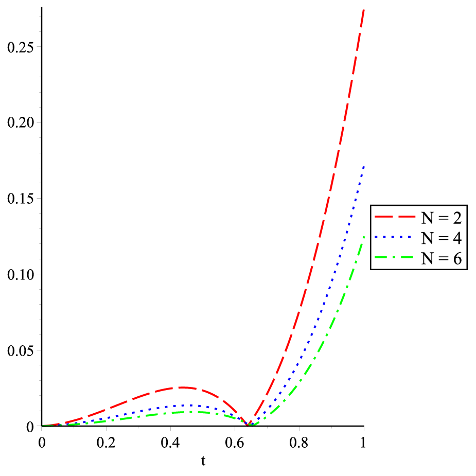
We consider the approximations given in Theorems 10, 12 and 13, with a fixed $n=1$ and $N\in\{2,4,6\}$ . The error of approximating $f(t)$ by $\tilde{f}(t)$ is measured by $|f(t)-\tilde{f}(t)|$ . See Figures 2–7.

5 Applications

In this section we apply the proposed technique to some concrete fractional differential equations of physical relevance.

5.1 A time-fractional diffusion equation

We extend the one-dimensional time-fractional diffusion equation [14] to the variable order case. Consider $u=u(x,t)$ with domain $[0,1]^{2}$ . The partial fractional differential equation of order ${\alpha(t)}$ is the following:

{{}^{C}_{0}\mathbb{D}_{t}^{{\alpha(t)}}u}(x,t)-\frac{\partial^{2}u}{\partial x^{2}}(x,t)=f(x,t)\hskip 10.00002pt\mbox{ for }\,x\in[0,1],\hskip 10.00002ptt\in[0,1],

(8)

subject to the boundary conditions

u(x,0)=g(x),\hskip 10.00002pt\mbox{ for }\,x\in(0,1),

(9)

and

u(0,t)=u(1,t)=0,\hskip 10.00002pt\mbox{ for }\,t\in[0,1].

(10)

We mention that when ${\alpha(t)}\equiv 1$ , one obtains the classical diffusion equation, and when ${\alpha(t)}\equiv 0$ one gets the classical Helmholtz elliptic equation. Using Lemma 6, it is easy to check that

u(x,t)=t^{2}\sin(2\pi x)

is a solution to (8)–(10) with

f(x,t)=\left(\frac{2}{\Gamma(3-{\alpha(t)})}t^{2-{\alpha(t)}}+4\pi^{2}t^{2}\right)\sin(2\pi x)

and

g(x)=0

(compare with Example 1 in [14]). The numerical procedure is the following: replace ${{}^{C}_{0}\mathbb{D}_{t}^{{\alpha(t)}}u}$ with the approximation given in Theorem 10, taking $n=1$ and an arbitrary $N\geq 1$ , that is,

{{}^{C}_{0}\mathbb{D}_{t}^{{\alpha(t)}}u}(x,t)\approx At^{1-{\alpha(t)}}\frac{\partial u}{\partial t}(x,t)+\sum_{p=1}^{N}B_{p}t^{1-p-{\alpha(t)}}V_{p}(x,t)

with

\begin{split}A&=\displaystyle\frac{1}{\Gamma(2-{\alpha(t)})}\left[1+\sum_{l=1}^{N}\frac{\Gamma({\alpha(t)}-1+l)}{\Gamma({\alpha(t)}-1)l!}\right],\\ B_{p}&=\displaystyle\frac{\Gamma({\alpha(t)}-1+p)}{\Gamma(1-{\alpha(t)})\Gamma({\alpha(t)})(p-1)!},\\ V_{p}(x,t)&=\displaystyle\int_{0}^{t}\tau^{p-1}\frac{\partial u}{\partial t}(x,\tau)d\tau.\end{split}

Then, the initial fractional problem (8)–(10) is approximated by the following system of second-order partial differential equations:

At^{1-{\alpha(t)}}\frac{\partial u}{\partial t}(x,t)+\sum_{p=1}^{N}B_{p}t^{1-p-{\alpha(t)}}V_{p}(x,t)-\frac{\partial^{2}u}{\partial x^{2}}(x,t)=f(x,t)

and

\frac{\partial V_{p}}{\partial t}(x,t)=t^{p-1}\frac{\partial u}{\partial t}(x,t),\hskip 10.00002ptp=1,\ldots,N,

for $x\in[0,1]$ and for $t\in[0,1]$ , subject to the boundary conditions

u(x,0)=0,\hskip 10.00002pt\mbox{ for }\,x\in(0,1),

u(0,t)=u(1,t)=0,\hskip 10.00002pt\mbox{ for }\,t\in[0,1],

and

V_{p}(x,0)=0,\hskip 10.00002pt\mbox{ for }\,x\in[0,1],\hskip 10.00002ptp=1,\ldots,N.

Remark 18.

As was mentioned in Theorem 10, as $N$ increases, the error of the approximation decreases and the given approximation formula converges to the fractional derivative. Thus, in order to have a good accuracy for the method, one should take higher values for $N$ .

Remark 19.

We are not aware of similar methods to our, concerning variable fractional calculus, in order to compare the performance of the proposed method to other numerical approximation methods. For this reason, we decided to compare with the exact solution. In the available literature, using a discretization process, FDEs are solved as finite differences. Our technique is quite different: we rewrite the FDE as a system of ordinary differential equations, and then we can apply any known technique to solve it. Note that the reason why we stopped here with $N=6$ was to have an approximation that is enough close to the exact solution but still visually distinguishably (when we increase $N$ more, the approximation and the exact solution appear to be the same in the plots). In terms of performance of the method, it is roughly the same to put $N=6$ or bigger.

5.2 A fractional partial differential equation in fluid mechanics

We now apply our approximation techniques to the following one-dimensional linear inhomogeneous fractional Burgers’ equation of variable order (see [17, Example 5.2]):

{{}^{C}_{0}\mathbb{D}_{t}^{{\alpha(t)}}u}(x,t)+\frac{\partial u}{\partial x}(x,t)-\frac{\partial^{2}u}{\partial x^{2}}(x,t)=\frac{2t^{2-{\alpha(t)}}}{\Gamma(3-{\alpha(t)})}+2x-2,\hskip 10.00002pt\mbox{ for }\,x\in[0,1],\hskip 10.00002ptt\in[0,1],

(11)

subject to the boundary condition

u(x,0)=x^{2},\hskip 10.00002pt\mbox{ for }\,x\in(0,1).

(12)

Here,

F(x,t)=\frac{2t^{2-{\alpha(t)}}}{\Gamma(3-{\alpha(t)})}+2x-2

is the external force field. Burgers’ equation is used to model gas dynamics, traffic flow, turbulence, fluid mechanics, etc. The exact solution is

u(x,t)=x^{2}+t^{2}.

The fractional problem (11)–(12) can be approximated by

At^{1-{\alpha(t)}}\frac{\partial u}{\partial t}(x,t)+\sum_{p=1}^{N}B_{p}t^{1-p-{\alpha(t)}}V_{p}(x,t)+\frac{\partial u}{\partial x}(x,t)-\frac{\partial^{2}u}{\partial x^{2}}(x,t)=\frac{2t^{2-{\alpha(t)}}}{\Gamma(3-{\alpha(t)})}+2x-2

with $A$ , $B_{p}$ and $V_{p}$ , $p\in\{1,\ldots,N\}$ , as in Section 5.1. The approximation error can be decreased as much as desired by increasing the value of $N$ .

Acknowledgments

This work was supported by Portuguese funds through the Center for Research and Development in Mathematics and Applications (CIDMA) and The Portuguese Foundation for Science and Technology (FCT), within project UID/MAT/04106/2013. Tavares was also supported by FCT through the Ph.D. fellowship SFRH/BD/42557/2007; Torres by project PTDC/EEI-AUT/1450/2012, co-financed by FEDER under POFC-QREN with COMPETE reference FCOMP-01-0124-FEDER-028894. The authors are very grateful to three anonymous referees, for several comments and improvement suggestions.

References

[1] T. M. Atanackovic, M. Janev, S. Pilipovic and D. Zorica, An expansion formula for fractional derivatives of variable order, Cent. Eur. J. Phys. 11 (2013), no. 10, 1350–1360.
[2] A. Atangana and A. H. Cloot, Stability and convergence of the space fractional variable-order Schrödinger equation, Adv. Difference Equ. 2013, 2013:80, 10 pp.
[3] M. Caputo, Linear model of dissipation whose $Q$ is almost frequency independent – II, Geophys. J. R. Astr. Soc. 13 (1967), 529-539.
[4] A. V. Chechkin, R. Gorenflo and I. M. Sokolov, Fractional diffusion in inhomogeneous media, J. Phys. A 38 (2005), no. 42, L679–L684.
[5] S. Chen, F. Liu and K. Burrage, Numerical simulation of a new two-dimensional variable-order fractional percolation equation in non-homogeneous porous media, Comput. Math. Appl. 67 (2014), no. 9, 1673–1681.
[6] C. F. M. Coimbra, Mechanics with variable-order differential operators, Ann. Phys. (8) 12 (2003), no. 11-12, 692–703.
[7] C. F. M. Coimbra, C. M. Soon and M. H. Kobayashi, The variable viscoelasticity operator, Annalen der Physik 14 (2005), 378–389.
[8] M. Dalir and M. Bashour, Applications of fractional calculus, Appl. Math. Sci. (Ruse) 4 (2010), no. 21-24, 1021–1032.
[9] K. Diethelm, The analysis of fractional differential equations, Lecture Notes in Mathematics, 2004, Springer, Berlin, 2010.
[10] M. M. Džrbašjan and A. B. Nersesjan, Fractional derivatives and the Cauchy problem for differential equations of fractional order, Izv. Akad. Nauk Armjan. SSR Ser. Mat. 3 (1968), no. 1, 3–29.
[11] R. Herrmann, Folded potentials in cluster physics—a comparison of Yukawa and Coulomb potentials with Riesz fractional integrals, J. Phys. A 46 (2013), no. 40, 405203, 12 pp.
[12] R. Hilfer, Applications of fractional calculus in physics, World Sci. Publishing, River Edge, NJ, 2000.
[13] D. Ingman and J. Suzdalnitsky, Control of damping oscillations by fractional differential operator with time-dependent order, Comput. Methods Appl. Mech. Engrg. 193 (2004), no. 52, 5585–5595.
[14] Y. Lin and C. Xu, Finite difference/spectral approximations for the time-fractional diffusion equation, J. Comput. Phys. 225 (2007), no. 2, 1533–1552.
[15] J. A. T. Machado, M. F. Silva, R. S. Barbosa, I. S. Jesus, C. M. Reis, M. G. Marcos and A. F. Galhano, Some applications of fractional calculus in engineering, Math. Probl. Eng. 2010 (2010), Art. ID 639801, 34 pp.
[16] D. A. Murio and C. E. Mejía, Generalized time fractional IHCP with Caputo fractional derivatives, J. Phys. Conf. Ser. 135 (2008), Art. ID 012074, 8 pp.
[17] Z. Odibat and S. Momani, The variational iteration method: an efficient scheme for handling fractional partial differential equations in fluid mechanics, Comput. Math. Appl. 58 (2009), no. 11-12, 2199–2208.
[18] T. Odzijewicz, A. B. Malinowska and D. F. M. Torres, Fractional calculus of variations in terms of a generalized fractional integral with applications to physics, Abstr. Appl. Anal. 2012, Art. ID 871912, 24 pp. arXiv:1203.1961
[19] T. Odzijewicz, A. B. Malinowska and D. F. M. Torres, Variable order fractional variational calculus for double integrals, Proceedings of the 51st IEEE Conference on Decision and Control, December 10–13, 2012, Maui, Hawaii, Art. no. 6426489 (2012), pp. 6873–6878. arXiv:1209.1345
[20] T. Odzijewicz, A. B. Malinowska and D. F. M. Torres, Fractional variational calculus of variable order, in Advances in harmonic analysis and operator theory, 291–301, Oper. Theory Adv. Appl., 229, Birkhäuser/Springer Basel AG, Basel, 2013. arXiv:1110.4141
[21] T. Odzijewicz, A. B. Malinowska and D. F. M. Torres, Noether’s theorem for fractional variational problems of variable order, Cent. Eur. J. Phys. 11 (2013), no. 6, 691–701. arXiv:1303.4075
[22] P. W. Ostalczyk, P. Duch, D. W. Brzeziński and D. Sankowski, Order Functions Selection in the Variable-, Fractional-Order PID Controller, Advances in Modelling and Control of Non-integer-Order Systems, Lecture Notes in Electrical Engineering 320 (2015), 159–170.
[23] S. Pooseh, R. Almeida and D. F. M. Torres, Approximation of fractional integrals by means of derivatives, Comput. Math. Appl. 64 (2012), no. 10, 3090–3100. arXiv:1201.5224
[24] S. Pooseh, R. Almeida and D. F. M. Torres, Numerical approximations of fractional derivatives with applications, Asian J. Control 15 (2013), no. 3, 698–712. arXiv:1208.2588
[25] Yu. N. Rabotnov, Creep problems in structural members, North-Holland Series in Applied Mathematics and Mechanics, Amsterdam/London, 1969.
[26] L. E. S. Ramirez and C. F. M. Coimbra, On the variable order dynamics of the nonlinear wake caused by a sedimenting particle, Phys. D 240 (2011), no. 13, 1111–1118.
[27] M. R. Rapaić and A. Pisano, Variable-order fractional operators for adaptive order and parameter estimation, IEEE Trans. Automat. Control 59 (2014), no. 3, 798–803.
[28] S. G. Samko, A. A. Kilbas and O. I. Marichev, Fractional integrals and derivatives, translated from the 1987 Russian original, Gordon and Breach, Yverdon, 1993.
[29] S. G. Samko and B. Ross, Integration and differentiation to a variable fractional order, Integral Transform. Spec. Funct. 1 (1993), no. 4, 277–300.
[30] F. Santamaria, S. Wils, E. de Schutter and G. J. Augustine, Anomalous diffusion in Purkinje cell dendrites caused by spines, Neuron. 52 (2006), 635-648.
[31] K. Singh, R. Saxena and S. Kumar, Caputo-based fractional derivative in fractional Fourier transform domain, IEEE Journal on Emerging and Selected Topics in Circuits and Systems 3 (2013), 330–337.
[32] H. G. Sun, W. Chen and Y. Q. Chen, Variable order fractional differential operators in anomalous diffusion modeling, Physica A. 388 (2009) 4586-4592.
[33] N. H. Sweilam and H. M. AL-Mrawm, On the Numerical Solutions of the Variable Order Fractional Heat Equation, Studies in Nonlinear Sciences 2 (2011), 31–36.
[34] D. Valério and J. Sá da Costa, Variable order fractional controllers, Asian J. Control 15 (2013), no. 3, 648–657.
[35] T. Yajima and K. Yamasaki, Geometry of surfaces with Caputo fractional derivatives and applications to incompressible two-dimensional flows, J. Phys. A 45 (2012), no. 6, 065201, 15 pp.
[36] B. Zheng, $(G^{\prime}/G)$ -expansion method for solving fractional partial differential equations in the theory of mathematical physics, Commun. Theor. Phys. (Beijing) 58 (2012), no. 5, 623–630.
[37] P. Zhuang, F. Liu, V. Anh and I. Turner, Numerical methods for the variable-order fractional advection-diffusion equation with a nonlinear source term, SIAM J. Numer. Anal. 47 (2009), no. 3, 1760–1781.

Abstract

1 Introduction

2 Fractional calculus of variable order

2.1 Variable order Caputo derivatives for functions of one variable

Definition 1 (Riemann–Liouville fractional derivatives of order α⁡(t){\alpha(t)}—types I and II).

Definition 2 (Caputo fractional derivatives of order α⁡(t){\alpha(t)}—types I, II and III).

Theorem 3.

Proof.

Theorem 4.

Theorem 5.

Proof.

Lemma 6.

Proof.

Lemma 7.

2.2 Variable order Caputo derivatives for functions of several variables

Definition 8 (Partial Caputo fractional derivatives of variable order—types I, II and III).

Theorem 9.

3 Approximation of variable order Caputo derivatives

Theorem 10.

Proof.

Remark 11.

Theorem 12.

Proof.

Theorem 13.

Proof.

Remark 14.

Theorem 15.

Theorem 16.

Theorem 17.

4 An example

5 Applications

5.1 A time-fractional diffusion equation

Remark 18.

Remark 19.

5.2 A fractional partial differential equation in fluid mechanics

Acknowledgments

References

Definition 1 (Riemann–Liouville fractional derivatives of order ${\alpha(t)}$ —types I and II).

Definition 2 (Caputo fractional derivatives of order ${\alpha(t)}$ —types I, II and III).