Topological nature of nonlinear optical effects in solids

Introduction —

Under strong light irradiation, materials show electric polarization $\mathcal{P}$ or current $J=d\mathcal{P}/dt$ which are nonlinear functions of the electric field $E$. These nonlinear optical responses (NLORs) form one of the most important research fields in condensed matter physics [1, 2], since the nonlinearity often plays a crucial role in optical devices. NLORs are also of crucial importance for the solar cell action. The photo-current in a solar cell is usually described by two processes, i.e., the generation of electron-hole pairs or excitons, and the separation of electrons and holes by the potential gradient in the p-n junctions. A recent remarkable advance is the discovery of large efficiency of the solar cell action in perovskite oxides with noncentrosymmetric crystal structure [3, 4, 5, 6, 7]. One promising scheme that describes this phenomenon is the shift-current induced by the band structure without the inversion symmetry [8, 9, 10, 11].

While nonlinear optical processes described above involve high energy excited states, the ground state and low energy excited states are sometimes characterized by the topological nature of the Bloch wavefunctions. Specifically, the Berry connection and curvature of wave functions determine the ground state properties and the low energy transport phenomena. Such examples include ferroelectricity [12], quantum Hall effect [13, 14], anomalous Hall effect [15], spin Hall effect [16, 17], and topological insulators [18, 19, 20], and ideal dc conduction [21]. Quantum mechanical wavefunctions can be regarded as geometrical objects in the Hilbert space because the inner product and distance are defined for them. This is especially the case in solids, since the Bloch wavefunctions are grouped into several bands separated by the energy gaps, and each band $n$ is regarded as a manifold in the Hilbert space. This manifold is characterized by a connection $\bm{a}_{n}(\bm{k})$ that relates neighboring two wave functions in the crystal momentum ($k$-)space as

$\displaystyle\bm{a}_{n}(\bm{k})=-i\langle u_{n\bm{k}}|\nabla_{\bm{k}}u_{n\bm{k}}\rangle$

(1)

where $|u_{n\bm{k}}\rangle$ is the periodic part of the Bloch wave function. One can also extend this concept to a generalized space including some parameters $Q$’s characterizing the Hamiltonian such as the atomic displacement. Equation (1) has the meaning of the intracell coordinates [22] where the real-space coordinate $\bm{x}_{c}$ of the wavepacket made from the Bloch wavefunctions near $\bm{k}$ is represented by

$\displaystyle x^{\mu}_{c}=i\frac{\partial}{\partial k_{\mu}}-a^{\mu}_{n}(\bm{k}).$

(2)

The second term comes from the nontrivial connection of the manifold for the band $n$ and upgrades the usual derivative in $\bm{k}$ to the gauge covariant derivative which is physically observable. Although $a^{\mu}_{n}(\bm{k})$ is a gauge dependent quantity (subject to a change of phases of wave functions), this correction can be understood as a band-dependent shift of the electron position arising from different linear combinations of atomic orbitals in the unit cell [22]. It is noted here that the vector potential $a^{\mu}_{n}(\bm{k})$ is related to the real space position because of the canonical conjugation relationship between $\bm{x}$ and $\bm{k}$.

The quantum Hall effect is a famous example where geometry of wave functions plays a crucial role in the low-energy transport. The Hall conductivity $\sigma_{xy}$ can be represented by the integral of the Berry curvature $\mathcal{F}_{n}(\bm{k})\equiv[\nabla_{\bm{k}}\times\bm{a}_{n}(\bm{k})]_{z}$ over the occupied states [13]. In the case of insulator, the integral with respect to $\bm{k}$ over the first Brillouin zone is quantized and called the Chern number. This leads to the quantized $\sigma_{xy}$, i.e., (integer) quantum Hall effect. Replacing one of the momentum, e.g., $k_{y}$, by some parameter $Q$ characterizing the Hamiltonian, $\sigma_{xy}$ turns into the electric polarization induced by the change in $Q$ [12]. A nonvanishing Chern number in $\bm{k}$-$Q$ space is tied to the quantum pumping [14].

However, these topological characterizations have been limited to ground state properties or linear responses to the weak external stimuli of low frequency. This is because NLORs involve higher energy excitations such as particle-hole pairs which drive the quantum state out of the ground state manifold. Conventional descriptions of the nonlinear responses are given by nonlinear susceptibility tensors $\chi$’s whose independent components are specified by the crystal symmetry and time-reversal symmetry. Microscopically, $\chi$’s have complex expressions including many matrix elements of the dipole moment along with energy denominators. These expressions usually do not give much information except for the trivial fact that the nonlinear responses show a resonance effect when the energy of light is nearly equal to the energy difference between the two states connected by the matrix elements. The topological nature of responses to the strong and/or high frequency stimuli have not been explored thus far except for a few cases.

The shift-current is one of such a few nonlinear phenomena whose geometrical meaning has been studied. The photo-current is the current induced by light irradiation as is well known. The induced photo-current $J$ is usually proportional to $E^{3}$ when the system preserves the inversion symmetry. However, when the system lacks the inversion symmetry, the photo-current $J$ can be proportional to $E^{2}$ and it is called “shift-current”. von Baltz and Kraut [8] have derived a formula for this shift-current, and related it to the intracell coordinates mentioned above. Specifically, it is expressed in terms of the phase $\varphi_{ij}(\bm{k})$ of the velocity matrix element $v_{ij}(\bm{k})$ between the valence and conduction bands, and the Berry connection $\bm{a}_{n}(\bm{k})$ as

	$\displaystyle\bm{J}\propto$	$\displaystyle E^{2}\int d\bm{k}\delta(\epsilon_{1}(\bm{k})-\epsilon_{2}(\bm{k})+\hbar\omega)$
		$\displaystyle\times|v_{12}(\bm{k})|^{2}\left[\nabla_{\bm{k}}\varphi_{12}(\bm{k})+\bm{a}_{1}(\bm{k})-\bm{a}_{2}(\bm{k})\right],$		(3)

where the subscripts 1 and 2 refer to the valence band and the conduction band, respectively, $\epsilon_{i}(\bm{k})$ is the energy of the band, and $\hbar\omega$ is the energy of the incident light. Note that this expression is gauge invariant due to the combination of $\nabla_{\bm{k}}\varphi_{12}(\bm{k})$ and $\bm{a}_{1,2}(\bm{k})$, and it is remarkable in a sense that the vector potential itself appears in the physical quantities. It is considered as a candidate mechanism of the high efficiency photovoltaic current in the solar cell action without the p-n junction  [3, 4, 5, 6, 9, 10, 7, 11]. We note that the photovoltaic Hall effect of two-dimensional Dirac fermions, e.g., in graphene, has also been studied as a topological phenomenon [23, 24, 25, 26, 27], where the circularly polarized light induces the Hall conductance $\sigma_{xy}$ proportional to $E^{2}$. In this case, the current $J$ is the third order effect, i.e., $\propto E^{3}$. It is shown that the light induced $\sigma_{xy}$ is expressed by a similar formula to that for the linear response; the only modification in the expression for $\sigma_{xy}$ is that $\mathcal{F}_{n}(\bm{k})$ and the Fermi distribution function are replaced by those of the nonequilibrium Floquet bands.

In this paper, we study the topological nature of the nonlinear optical responses by employing the Floquet two band models. This formalism offers a general description of nonlinear responses when the following conditions are met: (i) only one frequency $\Omega$ is involved (the monochromatic light), (ii) mostly two bands are involved in the optical transitions, and (iii) a steady state is achieved. We show that nonlinear optical responses of the even order of the external electric field $E$, such as photovoltaic effects and second harmonic generations, have geometrical meaning and are characterized by the Berry connection in a generalized space including both the momentum $\bm{k}$ and parameters $Q$’s. In particular, we point out that these topological description is applicable for general noncentrosymmetric crystals that support the even order nonlinear responses. We also discuss that nonlinear dc Hall responses, which are nonlinear responses in the odd order of $E$ in general, are related to the Berry curvature of Floquet bands. (It is noted however, that the topological description is limited to the dc output in this case of odd order responses.) Moreover, we classify the nonlinear processes according to the presence or absence of the inversion ($P$) and time-reversal ($T$) symmetries in terms of the Berry connection and the Berry curvature. In order to demonstrate our general discussions, we apply our formalism to a 1D model with inversion symmetry breaking which is a simple model of ferroelectric materials. By doing so, we clarify the topological nature of a few nonlinear responses and the symmetry constraints to the nonlinear responses in an explicit way.

Results:

Floquet two band model — We study nonlinear current responses by employing the Keldysh Green’s function method combined with the Floquet formalism [28, 29, 30, 31]. (See Materials and Methods for details of the formalism.) We focus on the two bands involved in the transition induced by the monochromatic light with the electric field $E(t)=Ee^{-i\Omega t}+E^{*}e^{i\Omega t}$. By using the Floquet bands, one can describe the nonequilibrium steady state as an anticrossing of a valence band dressed with one photon and a conduction band dressed with no photon, which is schematically shown in Fig. 1. The anticrossing of these two Floquet bands is captured by the following Hamiltonian (the convention $\hbar=1,e=1$ is used hereafter):

$\displaystyle H_{F}$

$\displaystyle=\begin{pmatrix}\epsilon^{0}_{1}+\Omega&-iA^{*}v^{0}_{12}\\ iAv^{0}_{21}&\epsilon^{0}_{2}\end{pmatrix}\equiv\epsilon+{\bm{d}}\cdot{\bm{\sigma}},$

(4)

where the subscripts 1 and 2 refer to the valence band and conduction band, respectively, $\epsilon^{0}$ is the original energy dispersion (for $E=0$), $A=E/\Omega$ and $v^{0}=\partial H_{0}(A=0)/\partial k$. The dc current operator is given by

$\displaystyle\tilde{v}$

$\displaystyle=\frac{\partial H_{F}}{\partial k}\begin{pmatrix}v^{0}_{11}&-iA^{*}\left(\frac{\partial v^{0}}{\partial k}\right)_{12}\\ iA\left(\frac{\partial v^{0}}{\partial k}\right)_{21}&v^{0}_{22}\end{pmatrix}\equiv b_{0}+{\bm{b}}\cdot{\bm{\sigma}}.$

(5)

Physical quantities are obtained from the lesser Green’s function which is given for the two band model as

$\displaystyle G^{<}$

$\displaystyle=\frac{(\omega-\epsilon+i\Gamma/2+{\bm{d}}\cdot{\bm{\sigma}})\Sigma^{<}(\omega-\epsilon-i\Gamma/2+{\bm{d}}\cdot{\bm{\sigma}})}{[(\omega-\epsilon+i\Gamma/2)^{2}-d^{2}][(\omega-\epsilon-i\Gamma/2)^{2}-d^{2}]}.$

(6)

Here the lesser self-energy is given by $\Sigma^{<}=i\Gamma(1+\sigma_{z})/2$. This form of $\Sigma^{<}$ assumes that the system couples to a heat bath which has a uniform energy spectrum and the Fermi energy lying within the the energy gap of the system. Thus we obtain the dc current expectation value as

$\displaystyle J$

$\displaystyle=-i\textrm{Tr}(\tilde{v}G^{<})=\int d\bm{k}(j_{1}+j_{2}+j_{3}),$

(7)

with

	$\displaystyle j_{1}$	$\displaystyle=\frac{\frac{\Gamma}{2}(-d_{x}b_{y}+d_{y}b_{x})}{d^{2}+\frac{\Gamma^{2}}{4}},$		(8)
	$\displaystyle j_{2}$	$\displaystyle=\frac{(d_{x}b_{x}+d_{y}b_{y})d_{z}}{d^{2}+\frac{\Gamma^{2}}{4}},$		(9)
	$\displaystyle j_{3}$	$\displaystyle=\frac{(d_{z}^{2}+\frac{\Gamma^{2}}{4})b_{z}}{d^{2}+\frac{\Gamma^{2}}{4}}+b_{0},$		(10)

where Tr denotes an integration over $\omega$ and $k$ and a trace for two by two matrices.

The first term $j_{1}$ in Eq. (7) can be written with the Berry phase as follows. First we write the denominator as

	$\displaystyle-d_{x}b_{y}+d_{y}b_{x}$	$\displaystyle=\textrm{Im}[(d_{x}+id_{y})(b_{x}-ib_{y})]$
		$\displaystyle=|A|^{2}\textrm{Im}\left[v^{0}_{21}\left(\frac{\partial v^{0}}{\partial k}\right)_{12}\right],$		(11)

with the current operator $v^{0}$ for the system without driving by $E$. In the two band model, the matrix element of $\frac{\partial v^{0}}{\partial k}$ is written as

	$\displaystyle\left(\frac{\partial v^{0}}{\partial k}\right)_{12}$	$\displaystyle=\frac{\partial v^{0}_{12}}{\partial k}-\langle\partial_{k}u_{1}|v^{0}|u_{2}\rangle-\langle u_{1}|v^{0}|\partial_{k}u_{2}\rangle$
		$\displaystyle=v^{0}_{12}\left[\frac{\partial}{\partial k}\log v^{0}_{12}+ia_{1}-ia_{2}+\frac{v^{0}_{11}-v^{0}_{22}}{\epsilon_{1}-\epsilon_{2}}\right],$		(12)

with $a_{i}=-i\langle u_{i}|\partial_{k}u_{i}\rangle$. Here, we used the identity $|u_{1}\rangle\langle u_{1}|+|u_{2}\rangle\langle u_{2}|=1$ for the two band model, and $\langle u_{1}|\partial_{k}u_{2}\rangle=-v_{12}^{0}/(\epsilon_{1}-\epsilon_{2})$. Thus we obtains

	$\displaystyle d_{x}b_{y}-d_{y}b_{x}$	$\displaystyle=|A|^{2}|v^{0}_{12}|^{2}R_{k}$		(13)
	$\displaystyle R_{k}$	$\displaystyle=\left[\frac{\partial\varphi_{12}}{\partial k}+a_{1}-a_{2}\right],$		(14)

with $\varphi_{12}=\textrm{Im}(\log v^{0}_{12})$, since $a_{i}$ and $v^{0}_{ii}$ are real. The vector $R_{k}$ is called a shift vector, which measures the difference of intracell coordinate between two band involved in the resonance. We note that $R_{k}$ is a gauge invariant quantity, where the Berry connection accompanies the $k$-derivative of the velocity operator to compensate the nontrivial parallel translation for the Bloch wave functions in $k$. Then the contribution to the current expectation value is written as

	$\displaystyle j_{1}$	$\displaystyle=|A|^{2}\frac{\frac{\Gamma}{2}}{d_{z}^{2}+|A|^{2}|v^{0}_{12}|^{2}+\frac{\Gamma^{2}}{4}}|v^{0}_{12}|^{2}R_{k}.$
		$\displaystyle\cong\frac{\pi|E|^{2}}{\Omega^{2}}\frac{\frac{\Gamma}{2}}{\sqrt{\frac{|E|^{2}|v_{12}^{0}|^{2}}{\Omega^{2}}+\frac{\Gamma^{2}}{4}}}\delta(d_{z})|v^{0}_{12}|^{2}R_{k},$		(15)

where we have assumed in the second line that $\Gamma$ and $|Av_{12}^{0}|$ are much smaller than the energy dispersion. If we further assume sufficiently small electric fields ($|Av_{12}^{0}|\ll\Gamma$), this reduces to $j_{1}\cong\frac{\pi|E|^{2}}{\Omega^{2}}\delta(d_{z})|v^{0}_{12}|^{2}R_{k}$. The second term $j_{2}$ in Eq. (7) is rewritten by using $d_{x}b_{x}+d_{y}b_{y}=|A|^{2}\textrm{Re}[v^{0}_{21}(\frac{\partial v^{0}}{\partial k})_{12}]$ as

$\displaystyle j_{2}=\frac{|A|^{2}\textrm{Re}[v^{0}_{21}(\frac{\partial v^{0}}{\partial k})_{12}]d_{z}}{d^{2}+\frac{\Gamma^{2}}{4}}.$

(16)

This contribution vanishes after integration over $k$ in the presence of the time-reversal symmetry (TRS), because $j_{2}$ is odd under the TRS. This can be understood from Eq. (12) and the fact that $v_{ii}^{0}$ is odd under the TRS. In a similar way, the contribution of $j_{3}$ in Eq. (7) vanishes because $j_{3}$ is odd under the TRS.

To summarize, the photocurrent in the second order of $E$ is given by

$\displaystyle J=\frac{\pi|E|^{2}}{\Omega^{2}}\int d\bm{k}\delta(\epsilon_{1}^{0}-\epsilon_{2}^{0}+\hbar\omega)|v^{0}_{12}|^{2}\left[\partial_{k}\varphi_{12}+a_{1}-a_{2}\right],$

(17)

in the presence of the time-reversal symmetry, which reproduces the expression for the shift current [8, 32, 9]. While we have focused on the two band model, the result in Eq. (17) can be extended to general cases involving more energy bands by summing up contributions from any two bands satisfying the resonance condition. We note that higher order correction to the above formula is captured by the factor $\frac{\Gamma}{2}/\sqrt{\frac{|E|^{2}|v_{12}^{0}|^{2}}{\Omega^{2}}+\frac{\Gamma^{2}}{4}}$ in Eq. (15). This leads to a crossover of photocurrent from $J\propto E^{2}$ to $J\propto\Gamma E$ by increasing the intensity of the monochromatic light and describes the effect of saturation of excitations.

Second harmonic generation — The SHG is the nonlinear current response with the frequency $2\Omega$ induced by a monochromatic light $E(t)=Ee^{-i\Omega t}+E^{*}e^{i\Omega t}$. We show that the SHG is also described with geometrical quantity (i.e., Berry connections) in a similar manner to the shift current. Here we consider the interband contribution to the SHG that involves two energy bands in the optical transition. In this case, we can apply our approach based on the Floquet two band model. Specifically, the SHG is contributed by two types of optical processes and accordingly two Floquet two band models: $H_{F}$ in Eq. (4) and

$\displaystyle H_{F}^{\prime}$

$\displaystyle=\begin{pmatrix}\epsilon^{0}_{1}+2\Omega&-\frac{1}{2}(A^{*})^{2}\partial_{k}v^{0}_{12}\\ -\frac{1}{2}A^{2}\partial_{k}v^{0}_{21}&\epsilon^{0}_{2}\end{pmatrix}\equiv d_{0}^{\prime}+\bm{d^{\prime}}\cdot\bm{\sigma}.$

(18)

The Floquet formalism also offers a concise description of time-dependent current responses, which is given in Eq. (36) in the Method section. According to Eq. (36), a contribution to $J(2\Omega)$, which is the Fourier component of the current proportional to $e^{-2i\Omega t}$, is written as $-iv_{12}^{\prime}(G^{<})_{21}$ for each Floquet two band model, where $v^{\prime}$ are chosen so as to give the time-dependence of $e^{-2i\Omega t}$. This is achieved by $v_{12}^{\prime}=iA(\partial_{k}v^{0})_{12}$ in the case of $H_{F}$ and $v_{12}^{\prime}=v^{0}_{12}$ in the case of $H_{F}^{\prime}$. By using Eq. (48) for $(G^{<})_{21}$, the interband contribution to the SHG is written as

	$\displaystyle J(2\Omega)$	$\displaystyle\cong i\frac{E^{2}}{2\Omega^{2}}\int d\bm{k}|v^{0}_{12}|^{2}(\partial_{k}\varphi_{12}+a_{1}-a_{2})$
		$\displaystyle\qquad\times\left(-\frac{1}{d_{z}+\frac{i\Gamma}{2}}+\frac{1}{2(d^{\prime}_{z}+\frac{i\Gamma}{2})}\right),$		(19)

where we only kept nonvanishing terms in the presence of the TRS. In particular, if we focus on the contribution to the SHG by the interband resonance that involves a $\delta$-function with respect to the energy difference, such contribution is given by

	$\displaystyle J(2\Omega)$	$\displaystyle\cong\frac{\pi E^{2}}{2\Omega^{2}}\int d\bm{k}|v^{0}_{12}|^{2}R_{k}$
		$\displaystyle\qquad\times\left[-\delta(\epsilon^{0}_{1}-\epsilon^{0}_{2}+\Omega)+\frac{1}{2}\delta(\epsilon^{0}_{1}-\epsilon^{0}_{2}+2\Omega)\right].$		(20)

This indicates that the interband contribution to the SHG is characterized by the shift vector $R_{k}$ which is defined with Berry connections. Thus the SHG is generated by dynamics of excited electron-hole pair that experiences a shift of intracell coordinates in the transition between the valence and conduction bands and is naturally related to the Berry connection of the Bloch electron.

Third order nonlinear response — Now we proceed to the third order nonlinear responses which are described by

$\displaystyle J_{i}=\chi^{3}_{ij}E(\omega)E(-\omega)E_{j}(\omega=0).$

(21)

Here, the current $J_{i}$ is induced by the static electric field $E_{j}$ in the presence of pump laser light of the frequency $\omega$.

We focus on the nonlinear Hall response in the two-dimensional systems. The nonlinear Hall response is obtained by applying the linear response theory for the nonequilibrium steady states,

$\displaystyle\sigma_{xy}$

$\displaystyle=\int_{\textrm{BZ}}d^{2}\bm{k}\sum_{i}f_{i}({\bm{\nabla}}\times\widetilde{{\bm{a_{i}}}})_{z},$

(22)

and expanding it in the second power of $|E(\omega)|$ [23]. Here, the Berry connection $\widetilde{{\bm{a}}}$ is defined for the Floquet states that describes the nonequilibrium steady states, and $f_{i}$ is the occupation of the $i$th Floquet state. The wave functions of the Floquet two band model in Eq. (4) is given by

$\displaystyle u_{1}$

$\displaystyle=\begin{pmatrix}\cos\frac{\theta}{2}\\ \sin\frac{\theta}{2}e^{i\phi}\\ \end{pmatrix},$

$\displaystyle u_{2}$

$\displaystyle=\begin{pmatrix}-\sin\frac{\theta}{2}\\ \cos\frac{\theta}{2}e^{i\phi}\\ \end{pmatrix},$

(23)

with

$\displaystyle\cos\theta$

$\displaystyle=\frac{d_{z}}{d},$

$\displaystyle\phi$

$\displaystyle=\tan^{-1}\left(\frac{d_{y}}{d_{x}}\right)=\varphi_{21}.$

(24)

Then the Berry connections for Floquet bands $u_{1}$ and $u_{2}$ are given by

	$\displaystyle\widetilde{\bm{a_{1}}}$	$\displaystyle=\frac{1}{2}(1-\cos\theta){\bm{\nabla}}\phi+\cos^{2}\frac{\theta}{2}\bm{a_{1}}+\sin^{2}\frac{\theta}{2}\bm{a_{2}},$		(25)
	$\displaystyle\widetilde{\bm{a_{2}}}$	$\displaystyle=\frac{1}{2}(1+\cos\theta){\bm{\nabla}}\phi+\sin^{2}\frac{\theta}{2}\bm{a_{1}}+\cos^{2}\frac{\theta}{2}\bm{a_{2}},$		(26)

where $\bm{a_{1}}$ and $\bm{a_{2}}$ are Berry connections for the original bands with $E=0$. The occupations are $f_{1}=(1+\cos\theta)/2$, and $f_{2}=(1-\cos\theta)/2$, since $f_{i}=(-i\Sigma^{<}_{ii})/\Gamma$ with $-i\Sigma^{<}/\Gamma=(\sigma_{z}+1)/2$. The original Hall conductivity $\sigma_{xy}^{0}$ for $E=0$ is given by setting $\theta=0$. Then one can obtain the photo-induced part of the Hall conductivity $\sigma_{xy}^{p}\equiv\sigma_{xy}-\sigma_{xy}^{0}$ as

	$\displaystyle\sigma_{xy}^{p}$	$\displaystyle=\frac{1}{4}\int d^{2}\bm{k}\sin^{2}\theta[{\bm{\nabla}}\times({\bm{\nabla}}\phi+\bm{a_{2}}-\bm{a_{1}})]_{z}$
		$\displaystyle=\int d^{2}\bm{k}\frac{A^{2}|v^{0}_{12}|^{2}}{4(d_{z}^{2}+A^{2}|v^{0}_{12}|^{2})}\mathcal{F},$		(27)

where $\mathcal{F}\equiv({\bm{\nabla}}\times\bm{a_{2}}-{\bm{\nabla}}\times\bm{a_{1}})_{z}$. If we assume that $A$ is sufficiently small, the Hall conductivity is given by

$\displaystyle\sigma_{xy}^{p}$

$\displaystyle=\int d^{2}\bm{k}\frac{\pi E}{4\Omega}|v^{0}_{12}|\delta(d_{z})\mathcal{F}.$

(28)

We can include the effect of relaxation by replacing the denominator in Eq. (27) with $4(d_{z}^{2}+A^{2}|v^{0}_{12}|^{2}+\Gamma^{2})$, which leads to

$\displaystyle\sigma_{xy}^{p}$

$\displaystyle=\int d^{2}\bm{k}\frac{\pi E^{2}}{4\Gamma\Omega^{2}}|v^{0}_{12}|^{2}\delta(d_{z})\mathcal{F}.$

(29)

This photo-induced Hall conductivity is proportional to $E^{2}$ and describes the third order nonlinear response. It is also proportional to the relaxation time $1/\Gamma$ indicating that the nonlinear modulation arises from excited free electrons. Equation (28) corresponds to the case of $A|v^{0}_{12}|\gg\Gamma$, while Eq. (29) to the case of $A|v^{0}_{12}|\ll\Gamma$. Therefore these two equations describe the crossover from $\sigma_{xy}^{p}\propto E$ to $\propto E^{2}/\Gamma$ behaviors in a similar manner to the case of shift current. This photo-induced Hall response is zero when the $T$ symmetry is preserved, since the contributions of $\mathcal{F}$ at $\bm{k}$ and $-\bm{k}$ cancel each other in that case. It gives the correction to $\sigma_{xy}$ in the $T$-broken case by the photo-excitation where $\mathcal{F}$ is the difference of the Berry curvatures between conduction and valence bands. This effect is extended to the nonlinear Kerr rotation when the probe electric field $E(\omega=0)$ is replaced with that of nonzero frequency. In addition, it also expresses the effects which are finite even in the case of $T$-symmetric cases when one of $\bm{k}$-component is replaced by the parameter $Q$ characterizing the Hamiltonian. Before discussing this issue, let us introduce an explicit model to demonstrate the nonlinear optical responses.

Application to inversion broken 1D chains — We apply the formalism described above to a one-dimensional model described by

	$\displaystyle H_{0}=\sum_{i}$	$\displaystyle\frac{1+Q_{2}(-1)^{i}}{2}(e^{iFt}c_{i}^{\dagger}c_{i+1}+h.c.)$
		$\displaystyle+Q_{1}(-1)^{i}c_{i}^{\dagger}c_{i}+Q^{\prime}_{1}(-1)^{i}(e^{2iFt}c_{i}^{\dagger}c_{i+2}+h.c.),$		(30)

where $Q_{1}$ is the staggered onsite energy and $Q_{2}$ is the bond strength alternation. Note that the inversion symmetry is broken in the presence of both $Q_{1}$ and $Q_{2}$. This model is describing the one-dimensional organic conductors [33, 34, 35, 36]. This is also the simplest model of the ferroelectricity in perovskite materials where $Q_{1}$ corresponds to the energy level difference between the oxygen and metal ions, and $Q_{2}$ to the bond strength change due to the displacement of the ions [37]. In order to see the effect of $T$-symmetry breaking, we also introduced $Q^{\prime}_{1}$ which expresses complex hoppings between next nearest neighbors having opposite signs for two sublattices. The Hamiltonian in Eq.(30) is given in the $k$-space as

$\displaystyle H_{0}=\cos\frac{k}{2}\sigma_{x}+Q_{2}\sin\frac{k}{2}\sigma_{y}+(Q_{1}+Q^{\prime}_{1}\sin k)\sigma_{z},$

(31)

where ${\bm{\sigma}}$ are the Pauli matrices describing the degree of freedom of the two sublattices in the unit cell. Now let us apply an electric field $E$ to this 1D model. The Floquet Hamiltonian is given by

$\displaystyle H_{mn}(k)$

$\displaystyle=\begin{pmatrix}Q_{1}-n\Omega&0\\ 0&-Q_{1}-n\Omega\\ \end{pmatrix}\delta_{mn}+\begin{pmatrix}C_{mn}&A_{mn}\\ B_{mn}&-C_{mn}\end{pmatrix},$

(32)

with $A_{mn}=(t+Q_{2}/2)e^{-ik/2}J_{m-n}(-F/2)+(t-Q_{2}/2)e^{ik/2}J_{m-n}(F/2)$, $B_{mn}=(t+Q_{2}/2)e^{ik/2}J_{m-n}(F/2)+(t-Q_{2}/2)e^{-ik/2}J_{m-n}(-F/2)$, and $C_{mn}=Q_{1}^{\prime}J_{m-n}(F)(-i)^{m-n}[(-1)^{m-n}e^{ik}-e^{-ik}]/(2i)$, where $F=eEa/\Omega$ with lattice spacing $a$, and $J_{n}(x)$ is the $n$th Bessel function,

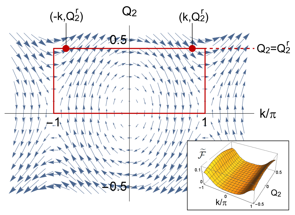
We can define $R_{Q_{2}}$ similar to $R_{k}$ in Eq. (14) by replacing the $k$-derivative with a $Q_{2}$-derivative. Then, we can consider the two-dimensional vector field $\widetilde{\bm{\mathcal{A}}}(k,Q_{2})=(\widetilde{\mathcal{A}}_{k},\widetilde{\mathcal{A}}_{Q_{2}})=|v^{0}_{12}|^{2}(R_{k},R_{Q_{2}})$ in the $(k,Q_{2})$-plane as plotted in Fig. 2. Taking the rotation of the vector field $\bm{R}$, one can get the flux distribution $\widetilde{\mathcal{F}}=|v^{0}_{12}|^{2}(\partial_{k}R_{Q_{2}}-\partial_{Q_{2}}R_{k})=|v^{0}_{12}|^{2}\mathcal{F}$ in the inset of Fig. 2. We note that $\widetilde{\mathcal{F}}$ is $|v^{0}_{12}|^{2}$ times the difference $\mathcal{F}\equiv\mathcal{F}_{2}-\mathcal{F}_{1}$ between the Berry curvatures of conduction and valence bands since the contribution from the phase of the transition matrix elements drops. These plots provide various information as follows. First, the sum of $A_{k}$ at $k$ and $-k$ satisfying the energy conservation law $E_{2}(\bm{k})-E_{1}(\bm{k})=\hbar\omega$ (indicated by two red dots in Fig. 2) corresponds to the shift-current $J$ proportional to $E^{2}$. Note that this sum does not vanish when $Q_{2}$ is nonzero, i.e., $P$ symmetry is broken. The corresponding quantity for $\widetilde{\mathcal{A}}_{Q_{2}}$ gives the change in the bond dimerization $B=\sum_{i}(-1)^{i}(c_{i}^{\dagger}c_{i+1}+h.c.)$ which is the “current” corresponding to the “vector potential” $Q_{2}$. However, as one can see from Fig. 2, the contributions from $k$ and $-k$ always cancel due to the $T$-symmetry.

Let us now turn to the Berry curvature. The integral of $\mathcal{F}$ over the “first-Brillouin zone” $-\pi<k<\pi$, $0<Q_{2}<Q^{r}_{2}$ ($Q^{r}_{2}$ is the realized value of the bond alternation), which is denoted by a red square in Fig. 2, is related to the polarization [12]. Namely, the integral of $\mathcal{F}_{1}$ over the first Brillouin zone is the polarization of the ground state. Therefore, that of $\mathcal{F}$ is the change of the polarization when all the electrons in the valence band are excited to the conduction band. The value of $\widetilde{\mathcal{F}}$ is related to the change in the bond dimerization $B$ defined above which is proportional to $E^{3}$. This third order nonlinear response of $B$ is obtained if $k_{y}$ is replaced by $Q_{2}$ in Eqs.(28) and (29) and the integration over $Q_{2}$ is dropped. This is intuitively understood as a “Hall response” of $B$ which is the “current” with respect to $Q_{2}$ and is transverse to the $k$-direction. In this case, there is no $Q_{2}$-integration because the contribution arises only from the realized value $Q_{2}^{r}$, and the photo-induced change of $B$ is given by the sum of $\mathcal{F}$ at $(k,Q_{2}^{r})$ and $(-k,Q_{2}^{r})$ with $\pm k$ satisfying the energy conservation law (indicated by two red dots in Fig. 2). As shown in the inset of Fig. 2, the values of $\mathcal{F}$ at $k$ and $-k$ are equal to each other, and hence this sum becomes nonvanishing. It is useful to note here that there is a very sensitive probe of $B$ in the case of molecular solids. The frequency shift of the intra-molecular vibrations detects the change of the valence state of each molecule [38]. We note that an anti-vortex in vector field $\widetilde{\bm{\mathcal{A}}}$ at $(k,Q_{2})=(\pm\pi,0)$ is attributed to the peak of the Berry curvature while a vortex at $(k,Q_{2})=(0,0)$ arises from the singularity in $v_{12}^{0}$ where $v_{12}^{0}$ vanishes and its phase is not well-defined.

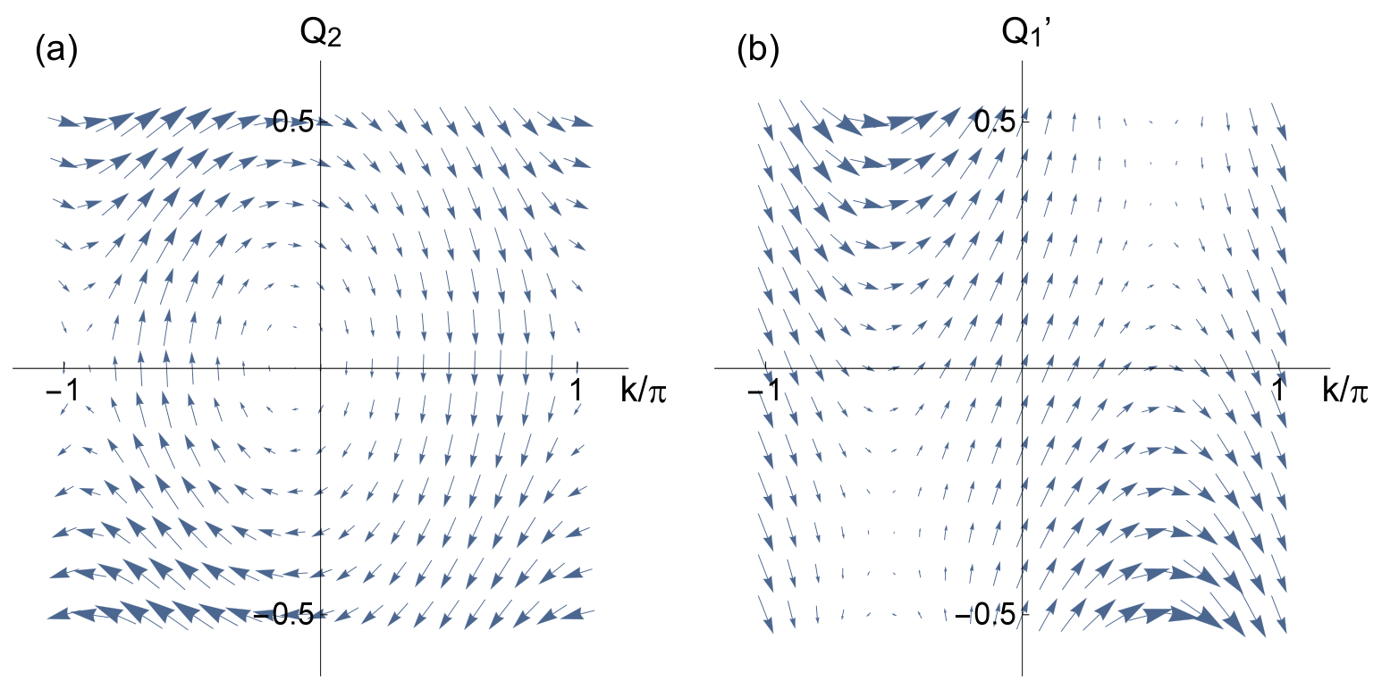
Next, we consider the effects of broken time-reversal symmetry $T$. Figure 3(a) shows the similar plots to Fig. 2 with finite $Q^{\prime}_{1}=0.1$. It is clearly seen that the symmetry between $k$ and $-k$ is broken and hence all the effects discussed above can be nonvanishing. For example, the photo-induced change in the bond dimerization proportional to $E^{2}$ becomes nonzero in addition to the shift current. We note that there is symmetry between $Q_{2}$ and $-Q_{2}$ which originates from the $PT$ symmetry as discussed in the next section. Figure 3(b) shows the vector field $(\widetilde{\mathcal{A}}_{k},\widetilde{\mathcal{A}}_{Q_{1}^{\prime}})$ with fixed $Q_{1}=1,Q_{2}=0.4$. While nonzero $Q_{1}$ and $Q_{2}$ break the $P$-symmetry, this figure demonstrates the role of $T$-symmetry. Namely, both $Q_{1}^{\prime}$ and $k$ change their sign under $T$, and the vector field in Fig. 3(b) obeys the constraint of the $T$ symmetry. The symmetry properties of various quantities will be discussed in the next section.

Discussion:

Symmetry considerations — Based on the results presented in the previous section, it is useful to summarize the symmetry properties. Figure 4 shows the transformation laws of the various quantities with respect to $P$ and $T$. Here, the parameter $Q$ breaks $P$ symmetry and reverses its sign under the $P$ operation while it remains unchanged under $T$. This is the case for $Q_{2}$ in the model Eq. (30). On the other hand, $\bm{k}$ goes to $-\bm{k}$ for both $P$ and $T$. The parameter $Q^{\prime}_{1}$ is also odd under both $P$ and $T$. The transformation properties of the Berry connection and the Berry curvature are summarized in Fig. 4. In particular, the presence or absence of the $T$-symmetry determines whether the effect of interest is allowed or not.

Let us study these transformation properties of $\bm{\widetilde{\mathcal{A}}}$ and $\widetilde{\mathcal{F}}$ in the 1D model in Eq. (30) below. First we discuss symmetry constraints on the vector fields in the $T$-symmetric case shown in Fig. 2. The action of $T$ constrains the vector field as $(\widetilde{\mathcal{A}}_{k}(-k,Q_{2}),\widetilde{\mathcal{A}}_{Q_{2}}(-k,Q_{2}))=(\widetilde{\mathcal{A}}_{k}(k,Q_{2}),-\widetilde{\mathcal{A}}_{Q_{2}}(k,Q_{2}))$, which is satisfied by two vectors at the two red dots in Fig. 2. Since the nonlinear responses are contributed both from $(k,Q_{2})$ and $(-k,Q_{2})$, the presence of the $T$-symmetry allows nonzero response associated with $\widetilde{\mathcal{A}}_{k}$ (shift current), but excludes that with $\widetilde{\mathcal{A}}_{Q_{2}}$ (nonlinear bond dimerization). Similarly, the vector fields in Fig. 2 is consistent with the constraint of the $P$-symmetry given by $(\widetilde{\mathcal{A}}_{k}(-k,-Q_{2}),\widetilde{\mathcal{A}}_{Q_{2}}(-k,-Q_{2}))=(-\widetilde{\mathcal{A}}_{k}(k,Q_{2}),-\widetilde{\mathcal{A}}_{Q_{2}}(k,Q_{2}))$. Since the flux distribution $\widetilde{\mathcal{F}}_{kQ_{2}}$ in the parameter space $(k,Q_{2})$ is even under both $T$ and $P$ as seen in the inset. Since the contributions at $k$ and $-k$ always add up, nonvanishing third order nonlinear response associated with $\widetilde{\mathcal{F}}_{kQ}$ is allowed. (We note that the nonlinear Kerr response is not allowed by the $T$-symmetry because contributions to $\widetilde{\mathcal{F}}_{k_{x}k_{y}}$ from $k$ and $-k$ cancel out.) Next, we consider the cases in Fig. 3 where the $T$-symmetry is broken due to nonzero $Q_{1}^{\prime}$. The vector field in Fig. 3(a) is not closed under either action of $T$ or $P$ because the fixed parameter $Q_{1}^{\prime}$ changes its sign, but it is closed under the combined $PT$ symmetry. From Fig. 4, the vector fields are constrained by the $PT$ symmetry as $(\widetilde{\mathcal{A}}_{k}(-k,-Q_{1}^{\prime}),\widetilde{\mathcal{A}}_{Q_{1}^{\prime}}(-k,-Q_{1}^{\prime}))=(\widetilde{\mathcal{A}}_{k}(k,Q_{1}^{\prime}),\widetilde{\mathcal{A}}_{Q_{1}^{\prime}}(k,Q_{1}^{\prime}))$, which is consistent with Fig. 3(a). In this case, both nonlinear responses associated with $\widetilde{\mathcal{A}}_{k}$ and $\widetilde{\mathcal{A}}_{Q_{2}}$ are allowed because the $T$-symmetry is no longer present. The vector field in Fig. 3(b) is not closed under the action of $P$ because the fixed parameter $Q_{2}$ changes its sign under $P$, but it is closed under the action of $T$; the $T$-symmetry constrains the vector field in Fig. 3(b). Under the action of $T$, the Berry connections $\widetilde{\mathcal{A}}_{k}$ and $\widetilde{\mathcal{A}}_{Q_{1}^{\prime}}$ are even as seen from Fig. 4. Thus the vector fields transform as $(\widetilde{\mathcal{A}}_{k}(-k,-Q_{1}^{\prime}),\widetilde{\mathcal{A}}_{Q_{1}^{\prime}}(-k,-Q_{1}^{\prime}))=(\widetilde{\mathcal{A}}_{k}(k,Q_{1}^{\prime}),\widetilde{\mathcal{A}}_{Q_{1}^{\prime}}(k,Q_{1}^{\prime}))$ which is consistent with Fig. 3(b).

Conclusions — We have studied the nonlinear optical responses from the topological properties based on the Keldysh + Floquet formalism taking into account the two states connected by the optical transition. The Berry connection and the Berry curvature appear in the even order and odd order responses in the electric field $E$ of the light, respectively. For example, the shift-current proportional to $E^{2}$ is represented by the Berry connection, while the Berry curvature appears in the third order response in $E$. These processes involve the excitation of electrons from the valence band to the conduction band, where created electrons and holes have been assumed to be non-interacting in this paper. In real materials, however, the electron correlation effect should be taken into account. In particular, the excitonic effect will hinder the photo-current generation. Therefore the many-body formulation of the nonlinear optical responses is an important issue to be studied in the future. As for the ferroelectric materials, however, the large dielectric constant screens the Coulomb effect and the excitonic effect is suppressed which may justify the single-particle treatment.

Acknowledgment — We thank Y. Tokura, M. Kawasaki, N. Ogawa, J. E. Moore, J. Orenstein and B. M. Fregoso for fruitful discussions. This work was supported by the EPiQS initiative of the Gordon and Betty Moore Foundation (TM), and by JSPS Grant-in-Aid for Scientific Research (No. 24224009, and No. 26103006) from MEXT, Japan, and ImPACT (Impulsing Paradigm Change through Disruptive Technologies) Program of Council for Science, Technology and Innovation (Cabinet office, Government of Japan) (NN).

Method:

Keldysh Green’s function—

The Keldysh Green’s function in the Floquet formalism is given by the Dyson equation [29, 31, 28, 23],

$\displaystyle\begin{pmatrix}G^{R}&G^{K}\\ 0&G^{A}\end{pmatrix}^{-1}_{mn}$

$\displaystyle=\begin{pmatrix}(\omega+n\Omega)\delta_{mn}-H_{mn}&0\\ 0&(\omega+n\Omega)\delta_{mn}-H_{mn}\end{pmatrix}+\Sigma_{mn},$

(33)

where $m,n$ run over the Floquet indices, and $\Sigma$ is the self energy. The Floquet Hamiltonian $H$ is obtained by expanding a Hamiltonian $H(t)$ periodic in time with period $T$ in the Floquet modes as

$\displaystyle H_{mn}$

$\displaystyle=\frac{1}{T}\int_{0}^{T}dte^{i(m-n)\Omega t}H_{0}(t),$

(34)

with $\Omega=2\pi/T$. We assume that each site is coupled to a heat reservoir with the Fermi distribution function $f(\epsilon)$ with a coupling constant $\Gamma$. In this case, the self energy is written as

$\displaystyle\Sigma_{mn}$

$\displaystyle=i\Gamma\delta_{mn}\begin{pmatrix}\frac{1}{2}&-1+2f(\omega+m\Omega)\\ 0&-\frac{1}{2}\end{pmatrix}.$

(35)

Then the current is given by

$\displaystyle J(t)$

$\displaystyle=\sum_{m}-i\textrm{Tr}[v(t)G^{<}_{mn}]e^{-i(m-n)\Omega t},$

(36)

where $v(t)$ is the time-dependent velocity operator defined by $v(t)=\partial H_{0}(t)/\partial k$ and Tr denotes an integration over $k$ and $\omega$ and a trace over band indices (but not over Floquet indices). We note that the reference Floquet index $n$ can be arbitrarily chosen due to the translation symmetry in the Floquet index. The lesser Green’s function $G^{<}$ is given by

	$\displaystyle G^{<}$	$\displaystyle=G^{R}\Sigma^{<}G^{A},$		(37)
	$\displaystyle\Sigma^{<}$	$\displaystyle=\frac{\Sigma^{R}+\Sigma^{K}-\Sigma^{A}}{2}.$		(38)

We note that the retarded and advanced Green’s functions are simply written as

$\displaystyle(G^{R/A})^{-1}_{mn}$

$\displaystyle=\left(\omega+n\Omega\pm\frac{i\Gamma}{2}\right)\delta_{mn}-H_{mn}.$

(39)

Furthermore, the dc part of the current $J$ is concisely obtained from the dc current operator defined from the Floquet Hamiltonian as

	$\displaystyle J$	$\displaystyle=\sum_{m}-i\textrm{Tr}[\tilde{v}_{nm}G^{<}_{mn}],$		(40)
	$\displaystyle\tilde{v}$	$\displaystyle=\frac{\partial H_{F}}{\partial k}.$		(41)

Lesser Green’s function for the Floquet two band model— In this section, we focus on the Floquet two band model and study the lesser Green’s function that is directly related to physical quantities.

First, we derive the Floquet Hamiltonian $H_{F}$ starting from the original Hamiltonian without a drive $H_{\textrm{orig}}(k)$. In the presence of the monochromatic light $E(t)=Ee^{-i\Omega t}+E^{*}e^{i\Omega t}$, the time-dependent Hamiltonian is given by

	$\displaystyle H_{0}(t)$	$\displaystyle=H_{\textrm{orig}}(k+A(t)),$		(42)
	$\displaystyle A(t)$	$\displaystyle=iAe^{-i\Omega t}-iA^{*}e^{i\Omega t},$		(43)

with $A=E/\Omega$. By keeping terms up to the linear order in $A$, one obtains

$\displaystyle H_{0}(t)$

$\displaystyle\cong H_{\textrm{orig}}(k)+A(t)v^{0},$

(44)

with $v^{0}=\partial H_{\textrm{orig}}/\partial k$. Next we express this time-dependent Hamiltonian as a Floquet Hamiltonian $(H_{F})_{mn}=H_{mn}-n\Omega\delta_{mn}$ by using Eq. (34). We further focus on two Floquet bands, i.e., the valence band with the Floquet index $n=-1$ and the conduction band with the Floquet index $n=0$. This leads to the two by two Floquet Hamiltonian

$\displaystyle H_{F}$

$\displaystyle=\begin{pmatrix}\epsilon^{0}_{1}+\Omega&-iA^{*}v^{0}_{12}\\ iAv^{0}_{21}&\epsilon^{0}_{2}\end{pmatrix}\equiv\epsilon+{\bm{d}}\cdot{\bm{\sigma}},$

(45)

where the subscripts 1 and 2 refer to the valence band and conduction band, respectively, and $\epsilon^{0}_{i}=(H_{\textrm{orig}})_{ii}$.

For this two by two Floquet Hamiltonian, the lesser Green’s function $G^{<}$ is obtained as follows. We consider the case where a coupling to a heat bath leads to the self energy given by Eq. (35). In this case, the retarded and advanced Green’s function are written as

$\displaystyle G^{R/A}$

$\displaystyle=\frac{\omega-\epsilon\pm i\Gamma/2+\bm{d}\cdot\bm{\sigma}}{(\omega-\epsilon\pm i\Gamma/2)^{2}-d^{2}}.$

(46)

Since the Fermi energy of the bath lies within the energy gap of the system, the Keldysh component of the self energy reduces to

$\displaystyle\Sigma^{<}$

$\displaystyle=i\Gamma\frac{1+\sigma_{z}}{2}.$

(47)

With these data, the lesser Green’s function for the Floquet two band model is obtained from Eq. (38). For example, an off-diagonal element of $G^{<}$ is given by

$\displaystyle(G^{<})_{21}$

$\displaystyle=\frac{(d_{x}+id_{y})\left(\frac{\Gamma}{2}+id_{z}\right)}{2\left(d^{2}+\frac{\Gamma^{2}}{4}\right)}.$

(48)

Here we note that the superscripts 21 indicate bases of the two by two Hamiltonian $H_{F}$ (with corresponding Floquet indices $0,-1$ ), and $(G^{<})_{21}$ describes the Fourier component of $e^{-i\Omega t}$ according to Eq. (36). Moreover, general expectation values are written as

	$\displaystyle\langle b_{0}+\bm{b}\cdot\bm{\sigma}\rangle$	$\displaystyle=-i\textrm{Tr}[(b_{0}+\bm{b}\cdot\bm{\sigma})G^{<}]$
		$\displaystyle=\frac{1}{d^{2}+\frac{\Gamma^{2}}{4}}\left[\frac{\Gamma}{2}(-d_{x}b_{y}+d_{y}b_{x})+(d_{x}b_{x}+d_{y}b_{y})d_{z}+\left(d_{z}^{2}+\frac{\Gamma^{2}}{4}\right)b_{z}\right]+b_{0}.$		(49)

References

- [1] N. Bloembergen, Nonlinear optics (World Scientific, Singapore, 1996).
- [2] R. W. Boyd, Nonlinear optics (Academic press, London, 2003).
- [3] I. Grinberg, D. V. West, M. Torres, G. Gou, D. M. Stein, L. Wu, G. Chen, E. M. Gallo, A. R. Akbashev, P. K. Davies, et al., Nature 503, 509 (2013).
- [4] W. Nie, H. Tsai, R. Asadpour, J.-C. Blancon, A. J. Neukirch, G. Gupta, J. J. Crochet, M. Chhowalla, S. Tretiak, M. A. Alam, H.-L. Wang, and A. D. Mohite, Science 347, 522 (2015).
- [5] D. Shi, V. Adinolfi, R. Comin, M. Yuan, E. Alarousu, A. Buin, Y. Chen, S. Hoogland, A. Rothenberger, K. Katsiev, Y. Losovyj, X. Zhang, P. A. Dowben, O. F. Mohammed, E. H. Sargent, and O. M. Bakr, Science 347, 519 (2015).
- [6] D. W. de Quilettes, S. M. Vorpahl, S. D. Stranks, H. Nagaoka, G. E. Eperon, M. E. Ziffer, H. J. Snaith, and D. S. Ginger, Science 348, 683 (2015).
- [7] A. Bhatnagar, A. R. Chaudhuri, Y. H. Kim, D. Hesse, and M. Alexe, Nat. Commun. 4, 2835 (2013).
- [8] R. von Baltz and W. Kraut, Phys. Rev. B 23, 5590 (1981).
- [9] S. M. Young and A. M. Rappe, Phys. Rev. Lett. 109, 116601 (2012).
- [10] S. M. Young, F. Zheng, and A. M. Rappe, Phys. Rev. Lett. 109, 236601 (2012).
- [11] A. M. Cook, B. M. Fregoso, F. de Juan, and J. E. Moore, arXiv:1507.08677 (2015).
- [12] R. Resta, Rev. Mod. Phys. 66, 899 (1994).
- [13] D. J. Thouless, M. Kohmoto, M. P. Nightingale, and M. den Nijs, Phys. Rev. Lett. 49, 405 (1982).
- [14] D. J. Thouless, Phys. Rev. B 27, 6083 (1983).
- [15] N. Nagaosa, J. Sinova, S. Onoda, A. H. MacDonald, and N. P. Ong, Rev. Mod. Phys. 82, 1539 (2010).
- [16] S. Murakami, N. Nagaosa, and S.-C. Zhang, Science 301, 1348 (2003).
- [17] J. Sinova, D. Culcer, Q. Niu, N. A. Sinitsyn, T. Jungwirth, and A. H. MacDonald, Phys. Rev. Lett. 92, 126603 (2004).
- [18] M. Z. Hasan and C. L. Kane, Rev. Mod. Phys. 82, 3045 (2010).
- [19] X.-L. Qi and S.-C. Zhang, Rev. Mod. Phys. 83, 1057 (2011).
- [20] C.-K. Chiu, J. C. Y. Teo, A. P. Schnyder, and S. Ryu, arXiv:1505.03535 (2015).
- [21] B. Hetényi, Phys. Rev. B 87, 235123 (2013).
- [22] E. Adams and E. Blount, J. Phys. Chem. Sol. 10, 286 (1959).
- [23] T. Oka and H. Aoki, Phys. Rev. B 79, 081406 (2009).
- [24] T. Kitagawa, T. Oka, A. Brataas, L. Fu, and E. Demler, Phys. Rev. B 84, 235108 (2011).
- [25] M. Sentef, M. Claassen, A. Kemper, B. Moritz, T. Oka, J. Freericks, and T. Devereaux, Nat. Commun. 6, 7047 (2015).
- [26] J. McIver, D. Hsieh, H. Steinberg, P. Jarillo-Herrero, and N. Gedik, Nat. Nanotech. 7, 96 (2012).
- [27] G. Jotzu, M. Messer, R. Desbuquois, M. Lebrat, T. Uehlinger, D. Greif, and T. Esslinger, Nature 515, 237 (2014).
- [28] S. Kohler, J. Lehmann, and P. Hänggi, Physics Reports 406, 379 (2005).
- [29] A.-P. Jauho, N. S. Wingreen, and Y. Meir, Phys. Rev. B 50, 5528 (1994).
- [30] K. Johnsen and A.-P. Jauho, Phys. Rev. Lett. 83, 1207 (1999).
- [31] A. Kamenev, arXiv:0412296 (2004), cond-mat/0412296 .
- [32] J. E. Sipe and A. I. Shkrebtii, Phys. Rev. B 61, 5337 (2000).
- [33] W. P. Su, J. R. Schrieffer, and A. J. Heeger, Phys. Rev. B 22, 2099 (1980).
- [34] M. J. Rice and E. J. Mele, Phys. Rev. Lett. 49, 1455 (1982).
- [35] N. Nagaosa and J. ichi Takimoto, J. Phys. Soc. of Jpn. 55, 2735 (1986).
- [36] S. Onoda, S. Murakami, and N. Nagaosa, Phys. Rev. Lett. 93, 167602 (2004).
- [37] T. Egami, S. Ishihara, and M. Tachiki, Science 261, 1307 (1993).
- [38] Y. Tokura, T. Koda, G. Saito, and T. Mitani, J. Phys. Soc. Jpn. 53, 4445 (1984).