Understanding Quantum Tunneling through Quantum Monte Carlo Simulations
Abstract
The tunneling between the two ground states of an Ising ferromagnet is a typical example of many-body tunneling processes between two local minima, as they occur during quantum annealing. Performing quantum Monte Carlo (QMC) simulations we find that the QMC tunneling rate displays the same scaling with system size, as the rate of incoherent tunneling. The scaling in both cases is , where is the tunneling splitting. An important consequence is that QMC simulations can be used to predict the performance of a quantum annealer for tunneling through a barrier. Furthermore, by using open instead of periodic boundary conditions in imaginary time, equivalent to a projector QMC algorithm, we obtain a quadratic speedup for QMC, and achieve linear scaling in . We provide a physical understanding of these results and their range of applicability based on an instanton picture.
Quantum annealing [1, 2, 2, 4, 5, 6] (QA) has been proposed as a method to solve combinatorial optimization problems. In contrast to its closely related classical counterpart, simulated annealing (SA) [7], which makes use of thermal fluctuations to escape local minima of the energy landscape in the search for a low energy solution, QA can additionally exploit quantum tunneling. In QA the system closely follows the ground state of a time-dependent Hamiltonian whose initial ground state at is easy to prepare. The final Hamiltonian encodes the cost function of a combinatorial optimization problem.
Random ensembles of hard problems are closely connected to spin glass models known in statistical physics. There one typically passes through a second order quantum phase transition from a paramagnetic into a glassy phase, where the energy gap closes polynomially with problem size , and then encounters a cascade of avoided level crossings with typically exponentially small gaps inside the glassy phase [2, 8, 9, 10]. In other problems, such as Grover search or number partitioning, there may just be a single exponentially small gap at a single first order quantum phase transition. Avoided level crossings with exponential gaps are the main bottleneck in quantum annealing and are in most cases associated with tunneling processes.
Simulations are important to understand the mechanisms of QA and find the class of problems for which QA may perform better than SA and other classical algorithms. QMC simulations have been performed [2, 11, 12] on problems of much larger sizes than accessible by direct integration of the time dependent Schrödinger equation. In particular, a recent numerical study of random Ising spin glass instances [12] has reconciled expectations of quantum speedup based on QMC simulations [2] with experiments that failed to detect it [5].
The major bottlenecks of QMC simulations of QA are also associated with tunneling events. However, while QMC faithfully samples the equilibrium thermal state of a quantum system it does not directly simulate its unitary time evolution. In particular, the universal critical exponents at second order quantum phase transitions are different than those of the stochastic QMC dynamics, as was recently pointed out in this context [13]. Nevertheless, correlations between QMC dynamics and the gap have recently been observed in simple models [14].
In this Letter we show that despite the different dynamics there exists a broad class of tunneling problems where QMC is not “merely” a quantum-inspired classical optimization algorithm [2, 4, 5]. In these problems the time of QMC to simulate quantum mechanical tunneling scales identically (in leading exponential order) with the problem size to the tunneling rate of a physical system and QMC is thus a quantitatively faithful predictor of QA performance. We also discuss possible types of problems where this may not apply.
Tunneling decay of a metastable state — To gain insight into the equivalence of QA and QMC we consider the tunneling between two nearly degenerate minima and of a potential . The pioneering work of Langer [15, 16] makes an explicit connection between the tunneling rate of a particle and the classical Kramers escape rate from the metastable state of a non-linear stochastic field process. This sheds light on how QA and QMC tunneling dynamics are related.
Within a semiclassical picture, the wave function decays exponentially in the classically forbidden region. In the particular case where the action under the barrier is purely imaginary this corresponds to a particle moving with imaginary momentum along the imaginary time axis [17, 18]. The amplitude of tunneling from the ground state associated with a local minimum is determined by the path integral = between the local minimum and the turning point at the barrier exit chosen to maximize . Here is the action of the path under the barrier and . The dominant contribution comes from the stationary action path (instanton) corresponding to a particle moving in the inverted potential . The tunneling amplitude is .
Similar arguments are known in statistical physics where the partition function of a state thermalized near a local minimum of the potential corresponds to the path integral in imaginary time with periodic boundary conditions for with . By tunneling away from the minimum, the partition function acquires an imaginary part. It is dominated by the instanton/anti-instanton path that moves under the barrier starting near , reaches the turning point , and returns [19]. We note that [20] gives a squared tunneling amplitude () because we pay the cost of creating an instanton and an anti-instanton.
In the context of QA we introduce a slowly varying field that changes the order of the minima of . At the start of QA the system is localized in the vicinity of and at the end it arrives at the vicinity of after a tunneling event at time when . In the case of open system QA when the dephasing time there is incoherent tunneling at from to with rate , determining the time scale of open system QA [21, 22, 23]. The same scaling with is also obtained in closed systems by the Landau-Zener formula.
Following Refs. [15, 16], the tunneling decay rate formally corresponds to the Kramers escape rate from a metastable state of a classical 1D field with order parameter satisfying the periodic boundary conditions and free energy functional . The stochastic evolution of this field in time is described by the Langevin equation , where is a random force delta correlated in both of its arguments and is a relaxation coefficient. We now observe that the same dynamics describes the standard path integral QMC to calculate the partition function . QMC samples paths with sweeping rate . The functional has a saddle point that the QMC trajectory crosses during the escape event from the metastable state towards . According to Kramers theory the escape rate is . This saddle point is precisely the instanton/anti-instanton path, and therefore the QMC escape rate . Therefore, in this archetypical example, the time needed for a physical system to tunnel is equal, within exponential accuracy, to the corresponding simulation time of quantum Monte Carlo.
We validated these arguments by simulations of tunneling in a one-dimensional double well potential , where depends exponentially on . Performing QMC simulations in continuous space [1] we compared the average QMC tunneling time to and find excellent agreeement over a wide range of time scales (see Supplementary Materials (SM)). Furthermore, we find that the QMC scaling does not significantly depend on whether local or global updates are used. Using open instead of periodic boundary conditions in imaginary time describes a so-called path integral ground state (PIGS) simulation [25]. There, the tunneling trajectory is dominated by configurations with a single instanton with corresponding escape rate – giving quadratic speedup of QMC over incoherent tunneling.
Tunneling in a transverse field Ising model — We now show that our findings are not limited to continuous variables, but extend to tunneling through barriers in quantum spin systems. To establish the equivalence of QA and QMC tunneling dynamics in this case we study the archetypical model of an Ising ferromagnet in the presence of a weak transverse field with Hamiltonian , considering both a linear chain with couplings and fully connected clusters with , where is the number of spins.
For small there are two degenerate ground states: the configuration labeled with spins aligned pointing (predominantly) up and average magnetization per site and the configuration labeled with . For finite the transverse field term mixes the two states with an exponentially small (in ) but nonzero tunneling matrix element . This lifts the degeneracy between the two ground states, resulting in an exponentially small energy gap between the states .

Adiabatically tuning a (weak) longitudinal field from a small positive to a small negative value, we encounter a tunneling problem, which is similar to the typical tunneling problem of QA at avoided level crossings, with the spins having to tunnel from to . This event is described by an instanton path in which all spins evolve in an identical fashion (see SM). The instanton dynamics can be described by an effective double well model, whose degenerate minima are located at (see Fig. 1).
We note that coupling to an environment could lead to thermally activated events, whose pathways traverses the high energy states with energy for a fully connected cluster and for a linear chain. These are suppressed by a factor and at low temperatures quantum tunneling becomes advantageous, as shown in Fig. 2).
Tunneling in path integral QMC — QMC simulations are performed by sampling imaginary time paths, obtained from a mapping of the partition function of a -dimensional quantum system to a -dimensional classical path integral configuration. For the transverse field Ising model this is just a classical Ising model in dimensions. -The path integral configurations consist of replicas of the same physical system with spins where the index denotes the spatial index and the index labels the time slices. Our QMC simulations have been performed both with a large number of replicas in order to be close to the physical continuous time limit, and also directly in the continuous time limit [26]. For updates we use variants of the Wolff [27] and Swendsen-Wang algorithm [28] to build local (in space) clusters along the imaginary time direction [29].
During the QMC simulation the total magnetization evolves stochastically in Monte Carlo time . Preparing the system in the vicinity of a local minimum, for example by choosing , most of the time all replicas sample spin configurations which are fluctuations around the same minimum energy configuration, i.e. . Every now and then the path evolves towards a transition state corresponding to the saddle point of the free energy functional of the classical spin model. Similar to the discussion in the continuous case, this saddle point corresponds to an instanton/anti-instanton pair (see Fig. 1 and SM). The instantonic path costs energy as it creates two domain walls in the imaginary time axis, which separate replicas which opposite magnetization . These domain walls can diffuse in opposite directions around the imaginary time loop, changing the total manetization to when they annihilate, signaling the completion of a tunneling event. The creation of represents the rate-limiting process of tunneling decay in both QMC and QA whose rate is .
To measure the tunneling time we start QMC simulations in a fully polarized state with and measure the number of QMC sweeps (defined as one attempted update per spin) required to obtain a well separated instanton/anti-instanton pair. We detect the latter by requiring that at least the of the replicas reverse their magnetization to 11 1 The number 25% is somewhat arbitrary but we find that waiting until all, or of the replicas reverse magnetization makes only small differences..

In Fig. 3 we show the measured average tunnelling time in QMC fully connected clusters as a function of and and observe an exponential scaling with . There is only a very weak temperature dependence for QMC in the low temperature quantum regime, mostly due to instanton diffusion. As shown in Fig. 3 the scaling of QMC simulations is identical to within error bars, thus confirming the identical scaling behavior of both types of dynamics. The same behavior is observed for linear chains (see SM).

Accelerating tunneling in QMC — Similar to the continuous case, we expect a quadratic speedup for PIGS simulations with open boundary conditions as in this case only one domain wall (instanton) is created in the magnetization reversing process (see Fig. 1). Indeed, as shown in Fig. 4 and Table I of SM the scaling exponent is reduced by a factor of two compared to QMC with periodic boundary conditions and open system QA, and the tunneling time now scales as instead of . PIGS algorithm can be viewed as projecting from a trial state (given by the boundary conditions in imaginary time) and sampling from the ground state wave function at large enough , hence providing the tunneling probability amplitude . This finding may explain the recently observed superiority of QMC projecting techniques compared to PIMC in continous space models [31].
Potential obstructions for QMC — While our findings apply to tunneling in a broad class of mean field models with purely imaginery time instantons, we shall also mention several areas where obstructions for the efficient simulation of quantum tunneling with QMC might exist.
QMC sampling may sometimes be inefficient due to topological obstructions such as winding numbers of world lines [32]. While PIGS simulations often solve this problem by cutting the periodic boundary conditions, an obstruction remains if the ground state wavefunction and its square are concentrated on different supports [32] – although suitable trial wave functions at the boundaries of the path integral can alleviate this problem. Conversely, the quantum system might have conserved quantum numbers that limit tunneling paths to a lower-dimensional subspace than that explored by QMC (see SM).
QMC may also be less efficient in optimization problems that require tunneling to or from multidimensional minima. In such problems the semiclassical action under the barrier is often not purely imaginary and displays complex features due to the presence of caustics, non-integrability and non-analyticity [33, 18]. Due to a highly oscillating nature of the wave function in the classically forbidden region it is not clear if the tunneling dynamics can be faithfully recovered with QMC.
Another important open question arises in problems that exhibit a many-body location/delocalization transition at finite values of transverse field [34]. There a delocalized phase can exist in a range of energies with exponentially many local minima separated by large Hamming distances and connected by a large number of tunneling paths [35]. QA, in contrast to QMC dynamics, may profit from the positive interference between exponentially many paths.
Conclusions — We conclude by discussing the consequences of our results for quantum annealing. Despite QMC dynamics being different from unitary evolution, the relevance of instanton configurations for tunneling processes in a class of models with purely imaginery time instantons leads to the same exponential scaling of tunneling rate through a tall barrier in both cases. A consequence of this equivalence is that QMC simulations are predictive of the performance of QA for hard optimization problems where the performance is limited by such tunneling events.
We also observed that is some cases a version of QMC with open boundary conditions (PIGS) can provide a quadratic speedup. While one can, theoretically, recover such a quadratic speedup [36] in QA if the evolution of the energy gap is exactly known and if the tunneling is fully coherent [22], this protocol can hardly be realized in practical QA. Nevertheless, a quadratic speed up can be achieved with polynomial overhead on a universal quantum computer using an approach that relaxes the above conditions [37].
These findings demonstrate that QMC simulations can be used as a powerful and predictive tool to investigate optimization problems amenable to quantum annealing. Our study demonstrates that the quest for quantum speedup using a physical quantum annealer must focus on the problems and hardware that allows to reach beyond the class of problems discussed in this paper where the identical scaling of QMC and QA preclude a scaling advantage and where PIGS can achieve a quadratic speedup for tunneling through individual barriers. The absence of calibration and programming errors, the flexibility in simulating arbitrary graph topologies without the need to embed into a hardware graph, and the observed quadratic speedup for tunneling through individual barriers in PIGS simulations makes QMC a competitive classical technology. Nevertheless, a physical QA can still be many orders of magnitude faster than QMC simulations [38]. We expect that the physical mechanisms behind the possible obstructions for QMC discussed above will provide interesting starting points for future studies of potential quantum speedup. In particular, one has to explore the power of QA with non-stoquastic Hamiltonians for which the negative sign problem prevents a matching QMC algorithm.
The work of GM and MT has been supported by the Swiss National Science Foundation through the National Competence Center in Research QSIT and by ODNI, IARPA via MIT Lincoln Laboratory Air Force Contract No. FA8721-05-C-0002. MT acknowledges hospitality of the Aspen Center for Physics, supported by NSF grant #PHY–1066293. We acknowledge useful discussions with F. Becca, M. Dykman, and G. Santoro.
References
- [1] T. Kadowaki and H. Nishimori, Phys. Rev. E 58, 5355 (1998).
- [2] E. Farhi, J. Goldstone, S. Gutmann, J. Lapan, A. Lundgren, and D. Preda, Science 292, 472 (2001).
- [3] G. E. Santoro, R. Martonak, E. Tosatti, and R. Car, Science 295, 2427 (2002).
- [4] S. Boixo, T. F. Ronnow, S. V. Isakov, Z. Wang, D. Wecker, D. A. Lidar, J. M. Martinis, and M. Troyer, Nature Physics 10, 218 (2014).
- [5] T. F. Rønnow, Z. Wang, J. Job, S. Boixo, S. V. Isakov, D. Wecker, J. M. Martinis, D. A. Lidar, and M. Troyer, Science 345, 420 (2014).
- [6] J. King, S. Yarkoni, M. M. Nevisi, J. P. Hilton, and C. C. McGeoch, arXiv:1508.05087 .
- [7] S. Kirkpatrick, C. D. Gelatt, and M. P. Vecchi, Science 220, 671 (1983).
- [8] B. Altshuler, H. Krovi, and J. Roland, Proceedings of the National Academy of Sciences 107, 12446 (2010).
- [9] E. Farhi, D. Gosset, I. Hen, A. W. Sandvik, P. Shor, A. P. Young, and F. Zamponi, Phys. Rev. A 86, 052334 (2012).
- [10] S. Knysh, arXiv:1506.08608 .
- [11] R. Martoňák, G. E. Santoro, and E. Tosatti, Phys. Rev. B 66, 094203 (2002).
- [12] B. Heim, T. F. Rønnow, S. V. Isakov, and M. Troyer, Science 348, 215 (2015).
- [13] C.-W. Liu, A. Polkovnikov, and A. W. Sandvik, Phys. Rev. Lett. 114, 147203 (2015).
- [14] L. T. Brady and W. van Dam, arXiv:1509.02562 .
- [15] J. S. Langer, Annals of Physics 41, 108 (1967).
- [16] J. S. Langer, Annals of Physics 54, 258 (1969).
- [17] S. Coleman, Phys. Rev. D 15, 2929 (1977).
- [18] S. Takada and H. Nakamura, J. Chem. Phys. 100, 98 (1994).
- [19] A. I. Vainshtein, V. I. Zakharov, V. A. Novikov, and M. A. Shifman, Soviet Physics Uspekhi 25, 195 (1982).
- [20] E. M. Chudnovsky and J. Tejada, Macroscopic Quantum Tunneling of the Magnetic Moment (Cambridge, UK: Cambridge University Press, 1998).
- [21] M. H. S. Amin and D. V. Averin, Phys. Rev. Lett. 100, 197001 (2008).
- [22] M. H. S. Amin, D. V. Averin, and J. A. Nesteroff, Phys. Rev. A 79, 022107 (2009).
- [23] S. Boixo, V. N. Smelyanskiy, A. Shabani, S. V. Isakov, M. Dykman, V. S. Denchev, M. Amin, A. Smirnov, M. Mohseni, and H. Neven, arXiv:1411.4036 .
- [24] D. M. Ceperley, Rev. Mod. Phys. 67, 279 (1995).
- [25] A. Sarsa, K. E. Schmidt, and W. R. Magro, J. Chem. Phys. 113, 1366 (2000).
- [26] H. Rieger and N. Kawashima, Eur. Phys. J. B 9, 233 (1999).
- [27] U. Wolff, Phys. Rev. Lett. 62, 361 (1989).
- [28] R. H. Swendsen and J.-S. Wang, Phys. Rev. Lett. 58, 86 (1987).
- [29] S. V. Isakov and R. Moessner, Phys. Rev. B 68, 104409 (2003).
- [30] The number 25% is somewhat arbitrary but we find that waiting until all, or of the replicas reverse magnetization makes only small differences.
- [31] E. Inack and S. Pilati, arXiv:1510.04650 .
- [32] M. B. Hastings, Quantum Information & Computation 13, 1038 (2013).
- [33] Z. H. Huang, T. E. Feuchtwang, P. H. Cutler, and E. Kazes, Phys. Rev. A 41, 32 (1990).
- [34] C. R. Laumann, R. Moessner, A. Scardicchio, and S. L. Sondhi, Eur. Phys. J. Special Topics 224, 75 (2015).
- [35] C. R. Laumann, A. Pal, and A. Scardicchio, Phys. Rev. Lett. 113, 200405 (2014).
- [36] J. Roland and N. J. Cerf, Phys. Rev. A 65, 042308 (2002).
- [37] S. Boixo, E. Knill, and R. D. Somma, arXiv:1005.3034 (2010).
- [38] V. Denchev et al., paper in preparation (2015).
Supplementary Materials for ”Understanding Quantum Tunneling through Quantum Monte Carlo Simulations”
I Path Integral Monte Carlo in continuous space
Imaginary time path integral Quantum Monte Carlo is a very well established technique for studying quantum statistical mechanics of many-particle realistic systems [1]. In this section we will briefly introduce path integral QMC in continuous space models. The formalism is very similar to the one introduced for spin models, the differences coming only from the different types of Hamiltonians. The typical real space Hamiltonian (in one dimension for sake of simplicity) is given by
| (1) |
where and are the position and momentum coordinate respectively, is the mass of the particle and is the potential. Here, the kinetic operator plays the role of the quantum fluctuation operator as in the transverse field Ising model. The strength of the quantum fluctuations is given by the particle’s mass . By applying the standard Trotter breakup for the density operator , the partition function at temperature is given by
| (2) |
where is the coordinate of the th system’s replica (time slice) and is the total number of Trotter replicas. Periodic boundary conditions applies, therefore . We refer the reader to Ref. [1] for additional details concerning energy estimators and more sophisticated Trotter breakups, i.e. more accurate approximate propagators. Eq. 2 represents the partition function of a classical ring polymer, made of beads at the fictitious temperature . Each replica is connected by harmonic springs whose spring constant is given by . This harmonic term represents the continuous model analogue of the ferromagnetic spin interaction between neighboring time slices in the transverse field model (see e.g. Ref. 2).
I.1 Path Integral Monte Carlo
The simplest way to sample is to perform Metropolis Monte Carlo moves on this extended system; the Metropolis weight being the integrand of Eq. 2. Even in the continuum case, updates can be local or global. The simplest local update consists in moving only one coordinate replica and accept/reject the move accordingly to the Metropolis algorithm. is a uniform random number in the range and is tuned in order to optimize the autocorrelation times. This is the kind of local update used in the main text. One MC sweep consists of local attempts. Clearly, many more global updates exist in which several replicas are moved at the same time. Global moves are extremely more efficient than the local ones for realistic many particles system [1, 3].
I.2 Path Integral Molecular Dynamics
Employing Molecular dynamics (MD) to sample the finite temperature canonical distribution of the ring polymer[3] is another way to perform global updates, which has no counterpart in spin models. In this case the forces are used to drive the sampling. Among all the possible MD integrator scheme we choose the Langevin equation of motions, because it represents a simple thermostat for sampling canonical distribution and allows ergodic sampling[4]. Adding the conjugate momenta to the coordinates, the ring polymer Hamiltonian reads
In order to sample the equilibrium distribution we integrate the (discretized) second order Langevin equation of motion
| (3) | |||||
| (4) |
where is the integration time step, is a Gaussian distributed random number, and includes all the forces acting on the -th replicas,
| (5) |
In this equation is a parameter which has to be tuned in order to minimize autocorrelation times and -in general- can also be position dependent. All the (collective) moves are accepted at the cost of introducing a time-step discretization error, which can be systematically removed in the limit . This is the kind of global update used in the main text.
I.3 Model, instanton detection and results
The simple onedimensional model considered in this work is given by the double well potential . The smaller the parameter the larger is the distance between the two wells, which goes as . The energy barrier also grows with decreasing , as . Therefore the control parameter in this toy model shares the same features as the system size for the transverse field Ising model, defined in the main text. Accurate energy gaps , between the ground and the first excited states, as a function of are calculated in Ref. [5] for the Hamiltonian , which can be used for direct comparison if we set the mass in the above equations. In this work spans between and which can provide a broad range of values, varying over 5 orders of magnitude. We choose the temperature in order to rule out thermally activated transitions. We set and . We start the simulations with all the replicas located at the bottom of the right well, i.e. . We identify the tunneling time in the following way: when the of the replicas exceed the coordinate we stop the simulation and record this passage time expressed as the number of MC sweeps (in the case of local updates with PIMC) or MD integration steps (for PIMD).

II Tunneling in ferromagnetic p-spin model
We first summarize the theory of tunneling in p-spin model closely following the theory developed in [6]. Consider the quantum Hamiltonian for an -qubit system corresponding to a ferromagnetic p-spin model in a transverse field
| (6) |
Here is the strength of the transverse field and the function is the mean-field potential energy of the spin system. We will consider the case where the function admits a metastable state and will be interested in the tunneling decay of this state at zero temperature. A well known example is given by the Curie-Weiss model where the function takes the form
| (7) |
where is a local field.
The Hamiltonian (6) is symmetric with respect to permutation of individual spins. To understand the structure of the eigenstates we use the total spin operators
| (8) |
The system Hamiltonian can be written in terms of these operators:
| (9) |
We are interested in the eigenstates of the Hamiltonian . They correspond to certain values of the total spin operator
| (10) |
which can take the following discrete values
| (11) |
The number of distinct irreducible subspaces of a given total spin is
| (12) |
each subspace has dimension . We will expand the eigenstates of in the basis of the operators and
| (13) |
where
| (14) | ||||
| (15) |
and the coefficients obey the stationary Schrödinger equation
| (16) |
(here we omitted the indices and .)
In what follows we will study the limit and assume that for the case of interest . We employ the discrete Wentzel-Kramers-Brillouin method developed in Ref. [7] applied to a mean-field model of a composite large spin [8, 6].
To the leading order in the parameter the stationary Schrödinger equation can be written in the form
where we omitted the indices and for brevity. Following the discrete WKB approach we write the wave function amplitudes as follows
| (17) | ||||
| (18) |
where the momentum obeys the classical Hamilton-Jacobi equation
| (19) |
We note that in the classically-allowed region, in the case relevant to us, and therefore
| (20) |
We now introduce the rescaled quantities
| (21) |
We note that with the above rescaling we must also introduce a new time variable . In order to satisfy the condition
| (22) |
we must set
| (23) |
Using (21) we write
| (24) |
We introduce the effective potential
| (25) |
This potential corresponds to the energies for the turning points of the classical trajectories of the system with the Hamiltonian function (24). The potential at different values of is depicted in the right panel of Fig. 2. It has a double well shape in certain parameter range of . We denote the extreme points of the potential as , which for k=1,2,3 correspond to the local minimum, maximum and global minimum respectively (cf. right panel of Fig. 2).

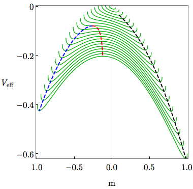
The imaginary momentum in the classically forbidden region under the barrier can be written in the form
| (26) |
We also note that in the classically forbidden region
| (27) |
The usual canonical relation between velocity and momentum has the form
| (28) |
(the minus sign here occurs because both the velocity and the momentum are purely imaginary under the barrier). From here we get
This expression also can be obtained from the Hamiltonian equation for coordinate . We write
| (29) | ||||
| (30) | ||||
| (31) |
For values of where metastability exists (cf. Fig. 2) we write the tunneling amplitude to logarithmic accuracy
| (32) | ||||
| (33) |
Here and are turning points of the instanton trajectory on different sides of the barrier that satisfy the condition
| (34) |
(the instanton trajectory at zero temperature has the energy of the local minimum).
II.0.1 Curie-Weiss model with zero bias
The Hamiltonian for the unbiased Curie-Weiss model corresponds to (6) and (7) with
| (35) |
At zero temperature the tunneling occurs exclusively within the subspace of the maximum total spin. The analytical expression for the tunneling splitting of the ground state energy can be derived in the asymptotical limit of large number of qubits and has a form derived by a number of authors in the past (see e.g. [7] )
| (36) | ||||
| (37) | ||||
| (38) |
Because we will be comparing the (doubled) scaling exponent (38) with the scaling exponent for the QMC tunneling rate obtained from the numerical simulations of the problems with limited values of it is important to understand the finite size effect coming from the prefactor in (37).
The left panel of Fig. 3 shows the -dependence of the ratio of the logarithm of the gap computed via the above analytical expression to that computed via the numerical diagonalization of the Hamiltonian (35). Similarly, the right panel of Fig. 3 shows the comparison between the scaling exponent (38) and the quantity computed via numerical diagonalization of . Note that in the later case the convergence with is while in the former it is .


Finally, Fig. 4 shows the dependence on of the exponent of the tunneling decay rate of the metastable state given by (32) (for zero basis the result is also computed by using (38) ).

II.1 Tunneling in the Grover problem
The Grover search problem can be recast in the adiabatic setting using the following Hamiltonian (see [9])
| (39) | ||||
| (40) |
This Hamiltonian can be rewritten in terms of the large spin operators (8) in the form (9) with the function
| (41) | ||||
| (42) |
where is the Kronnecker delta.
At the ground state of this Hamiltonian is , corresponding to all spins along the axis. The ground state energy is . At the ground state is with energy . At the avoided crossing occurs between the energies with the size of the energy splitting being
| (43) |
We now recast this result using the WKB approach described above. For the equation (24) takes the form . The corresponding effective potential is
In complete analogy to the discussion in the general case presented in the previous section the ground state wavefunction is localized at and decays exponentially away from this point. The tunneling path moves under the barrier and ends at the point . It is immediately clear that the tunneling path can only reach the target state for . In fact this also immediately follows from inspection of the Fig. 2 (right panel). While this figure is plotted for a different the common feature is that the tunneling path terminates at where the equality is reached only for .
At the avoiding crossing we solve the equation (31) for the instanton trajectory for and get
| (46) |
This trajectory approaches the solution state at as . The momentum (26) at the instanton trajectory under the barrier equals
| (47) |
With that the action (33) along the instanton is
| (48) |
Using (32) we recover the well-known quadratic speedup (43).
III Tunneling in path-integral QMC for ferromagnetic p-spin model
To describe the stochastic QMC process that samples paths over imaginary time in a spin system with the Hamiltonian (6) we define the state vector
| (49) |
In path integral QMC the trajectories satisfy periodic boundary conditions
| (50) |
In the PIGS version of QMC one uses open boundary conditions. There exists an order parameter corresponding to the z-component of the total magnetization
The probability functional for a realization of the trajectory equals
Above is a single-spin imaginary time propagator evaluated along the trajectory (see e.g. [10] for details). Marginalizing over the path configurations that corresponds to a given the probability functional can be written in the form (cf. [8])
| (51) |
| (52) |
where
| (53) | ||||
| (54) | ||||
| (55) |
The partition function is defined as usual as a normalization factor in the probability functional. In the above is a classical “gauge” field associated with .
This functional has “trivial” extremal points
| (56) |
corresponding to the extrema of the mean-field free energy function
| (57) |
| (58) |
For the sake of bookkeeping we assume that and correspond to local and global minima respectively,
| (59) |
The free energy functional values at the minima equal
| (60) |
During QMC a stochastic evolution of the system state (49) corresponds to a stochastic evolution of , where is Monte Carlo time. We initialize the system state at the vicinity of the local minimum of the free energy functional
Most of the time fluctuates near the local minimum. Escape from this minimum can be described in terms of the classic Kramers escape theory as was illustrated in the paper for the case of QMC with continuous variables. To logarithmic accuracy the escape rate is given by the Boltzmann factor
| (61) |
where we assumed that the Monte Carlo temperature equals 1. Here correspond to a nontrivial saddle point of the free energy functional satisfying
| (62) |
Using (53),(54) and (55) we obtain
| (63) |
where we dropped the argument above. We introduce a vector
| (64) |
Then after some transformations, using (53),(54), (55) we obtain
| (65) |
where
| (66) |
The above equations has intervals of motion
| (67) |
We set
| (68) |
where satisfies the equation
| (69) |
Upon inspection of the Eqs. (69),(24) and (26) one can see that up to the choice of the integrals of motion and the equation for coincides with that for the quantum instanton described in the previous section. In the zero-temperature limit of the value of must coincide with the local minimum of in . Then the choice of must be done in a way that the self-consistent equation (63) is satisfied.
Detailed calculation will be provided elsewhere [11]. One can show that in the zero temperature limit the value of and the WKB instanton for the tunneling at zero temperature precisely corresponds to the path that provides the saddle point of the free-energy functional (with time rescaling (23) taken into account). Similarly, the action along the WKB instanton trajectory equals to the difference of the values of between the saddle point and local minimum
| (70) |
Therefore at zero temperature the exponential scaling with the problem size of the QMC and quantum tunneling are the same.
IV QMC tunneling results for a ferromagnetic Ising chain
Here we report QMC simulations on a ferromagnetic Ising chain in the presence of a weak transverse field with Hamiltonian . The nearest neighbours couplings are given by .
We measure the average tunneling time for different sizes , i.e. the number of sites, as explained in the main text and compare these values with the inverse gap and inverse gap squared obtained with exact diagonalization.
In Figs. 5, 6, 7 we compare QMC simulations with periodic boundary conditions (PIMC), performed with different inverse temperatures and different transverse field values , against the inverse squared gap . In Figs. 8, 9, 10 we compare instead QMC simulations with open boundary conditions (PIGS) against the inverse gap . The complete exponential fit parameters are given in Table 1. The scaling of PIMC (PIGS) simulations compares well to () within error bars.
| ED | ||||
| QMC-PIMC | ||||
| 0.8 | 0.52(2) | 0.553(17) | 0.541(4) | 0.535(4) |
| 0.75 | 0.64(3) | 0.67(4) | 0.6697(14) | 0.662(4) |
| 0.7 | 0.78(2) | 0.80(3) | 0.81(5) | 0.799(4) |
| QMC-PIGS | ||||
| 0.8 | 0.270(12) | 0.281(11) | 0.289(11) | 0.268(2) |
| 0.75 | 0.329(11) | 0.341(11) | 0.350(9) | 0.331(2) |
| 0.7 | 0.397(9) | 0.410(9) | 0.417(9) | 0.400(2) |
| 0.65 | 0.462(11) | 0.477(8) | 0.482(18) | 0.473(2) |
| 0.6 | 0.540(10) | 0.556(19) | 0.56(2) | 0.553(2) |


References
- [1] D. M. Ceperley, Rev. Mod. Phys. 67, 279 (1995).
- [2] G. E. Santoro, R. Martonak, E. Tosatti, and R. Car, Science 295, 2427 (2002).
- [3] M. E. Tuckerman, B. J. Berne, G. J. Martyna, and M. L. Klein, J. Chem. Phys. 99, 2796 (1993).
- [4] G. Mazzola, S. Yunoki, and S. Sorella, Nature Communications 5, 3487 (2014).
- [5] K. Banerjee and S. P. Bhatnagar, Phys. Rev. D 18, 4767 (1978).
- [6] K. Kechedzhi and V. N. Smelyanskiy, arXiv:1505.05878 .
- [7] A. Garg, J. Math. Phys 39, 5166 (1998).
- [8] V. Bapst and G. Semerjian, Journal of Statistical Mechanics: Theory and Experiment 2012, P06007 (2012).
- [9] E. Farhi, J. Goldstone, S. Gutmann, and M. Sipser, quant-ph/0001106 .
- [10] F. Krzakala, A. Rosso, G. Semerjian, and F. Zamponi, Phys. Rev. B 78, 134428 (2008).
- [11] Z. Jiang, V. Smelyanskiy, S. V. Isakov, G. Mazzola, S. Boixo, M. Troyer, and H. Neven, On the equivalence between the instantons in quantum tunneling and path integral Monte Carlo simulations, in preparation (2015).