Dependent Random Density Functions with Common Atoms and Pairwise Dependence
Spyridon J. Hatjispyros ∗, Theodoros Nicoleris∗∗ and Stephen G. Walker∗∗∗
∗ Department of Mathematics, University of the Aegean,
Karlovassi, Samos, GR-832 00, Greece.
∗∗ Department of Economics, National and Kapodistrian University of Athens,
Athens, GR-105 59, Greece.
∗∗∗Department of Mathematics, University of Texas at Austin,
Austin, Texas 7812, USA.
1. Introduction. There has been substantial recent interest in the construction of dependent probability measures. We first restrict our thoughts to dependence between two random probability measures, and , though for the paper we are concerned with creating (pairwise) dependence between probability measures. To complete the motivation, the typical scenario in which such measures are employed is with mixture models, generating random densities and , whereby
The marginal models for each are a random density function based on the benchmark mixture of Dirichlet process model (Lo, 1984); so that each is a Dirichlet process (Ferguson, 1973), and is a density function for each . The reason for dependence is that it is thought that properties of and are similar in some way; for example the means are similar, or it is thought the distance between them is small, in that they resemble each other.
We can write each using the constructive definition of the Dirichlet process given in Sethuraman (1994); so that
where we write , being independent and identically distributed from some fixed distribution , with density function . And we write ; a stick–breaking process, so if all the are independent and identically distributed from the beta distribution, for some , then and, for ,
In applications, the and can be made dependent in a variety of ways. The modeling of dependent random Dirichlet processes has been the focus of much recent research in Bayesian nonparametrics; following original developments in MacEachern (1999). More recent work is to be found in De Iorio et al. (2004), Griffin and Steel (2006), Dunson and Park (2008) and summaries in Hjort et al. (2010). The use of the Dependent Dirichlet process arises mostly in regression problems where a random measure is constructed for each covariate and is of the type
where are processes of weights and atoms.
On the other hand, the work reported here is about modeling a finite number of densities, equivalent to the regression model with a finite number of fixed covariates. Previous work related to this type of structure is to be found in Müller et al. (2004) and Bulla et al. (2009), and more recently Hatjispyros et al. (2011), Kolossiatis et al. (2013) and Griffin et al. (2013). These papers model an arbitrary but finite number of random distribution functions, via a common component and an index specific idiosyncratic component. That is, the basic idea is to model
where is the common component to all other distributions and are the idiosyncratic parts, unique to each , . And are modeled as mutually independent mixture of Dirichlet process models, or based on some other stick–breaking process (Ishwaran and James, 2001) or normalized random measure as in the case of Griffin et al. (2013). In all these cases the (random) atoms for the underlying Dirichlet process are unique to each .
The present paper is concerned with constructing so that there is a unique common component for each pair with . This allows arbitrary pairwise dependence between any two and . The details of this idea for the case were presented in Hatjispyros et al. (2011). Our numeric results target the key case, which essentially gives access to arbitrary values of . It is clear that is a straightforward special case.
Moreover, our thesis is that when constructing e.g. and , it is sufficient to create a dependence between the weights and to take . That is, it is sufficient for the random probability measures and to have the same atoms. We demonstrate this sufficiency throughout the paper.
The key to the understanding of this idea is quite straightforward. From a fixed set of random atoms obtained for one probability measure, another probability measure can be obtained by reassigning the weights to these same atoms. It should be clear that varying weights can provide probability measures which are either remarkably close, when weights are similar, to probability measures which are far apart, when the weights are dissimilar.
It is less interpretable to have both varying weights and atoms. For if the weights are similar, there is nothing to be said about the closeness of the distributions as the ulimate picture will depend on the atoms. And we decide to make the atoms similar and allow the weights to vary so that with the same atoms we can easily compute distances between the two measures. We will look at this in Section 2.
We will demonstrate the idea using a dependent model suggested by Hatjispyros et al. (2011) for constructing pairwise dependence for the finite set of densities
where each is a random density function. The idea is that from each density we observe independent data sets, yet the densities from which they come share common features. For example, they may all have similar tail behaviour or even have common variances, and so on. Hence, it is imperative to model in the prior an arbitrary level of dependence between each pair , for each . The key is to construct the prior model in such a way that for every pair there is a “common” part and a “difference” part, to be explained more explicitly in due course.
The layout of the paper is as follows. In Section 2 we provide some preliminary findings concerned with the evaluation of distances between probability measures being generated. This is possible when atoms are common to each distribution. In section 3 we describe the model of interest and introduce the latent variables which will form the basis of the Gibbs sampler which is described in Section 4. Section 5 contains a numerical illustration involving a real data set and finally Section 6 concludes with a summary and future work.
2. Preliminaries. Given the common atoms for and we can easily compute distances between them and also between the corresponding mixed density functions. So, for suitable sets ,
Therefore, for the total variation distance between and we have
where, for example,
where is an index set. This is simple to interpret but impossible to obtain and control if the atoms are not identical. In fact, if the atoms are disjoint for each measure, close weights, even identical weights, says nothing about how close the two measures are to each other. We believe equal atoms is fundamental as a consequence.
We can formalize the idea of using common atoms and the sufficiency of this by considering the following
Lemma : We consider the densities and where the , and are fixed, and the are dense in . Then we can find such that the -distance between and can be made arbitrarily small.
Proof: Because the are dense in , for any and any , we can find and such that
We assume without loss of generality that is one to one, for . Then, we put , and for the remaining indices we set . Thus, we have that . Hence,
Now choose such that, for any , we have
and the lemma follows.
Thus, even though atoms are fixed across densities, as long as they form a dense set, we can approximate arbitrarily accurately any density with any atoms.
Hence, we can obtain weights to allow this distance to be either 0, the weights coincide, or to be 1. A dependent prior for can be used to provide a small distance between and if that is what is required. This is not so obvious to achieve if the atoms are dissimilar. Moreover, if atoms are dissimilar computing the informative distances is not possible and one is left with computing objects such as
which, although it provides some insight on the dependence between and , is not the appropriate learning tool for the similarity between two random densities. Clearly, in that case the total variation distance (or the distance between densities) is a more appropriate measure.
We now turn to looking at a distance between and , and for ease of computation we make this the distance,
Lemma : We consider the random mixtures with independent, coming from the base measure for all , then
where and .
Proof: It is that
where
Taking expectations over the atoms but keeping the weights fixed, we have
where
and note that . Now it is very easy to show that by utilizing the identities
and
and the lemma follows.
So, again, crucial distances can be understood solely through the weights.
If we are now interested in creating dependent weights for and (which will allow extensions to a larger number of densities with pairwise dependence), then we construct weights of the type
with . This gives a common part to and , via a common part to and , and we can write
due to the common atoms.
On the other hand, in Hatjispyros et al. (2011) the model was described as
with . It had to be like this due to the uncommon atoms of , and , i.e.
The details of the model where random probability measures share common atoms is now described in Section 3.
3. The model. We start off by describing the model as it was in Hatjispyros et al. (2011) and then proceed to detail the simplifications when atoms are common. So, we have the set of random density functions generated via
where . The random densities satisfy and are independent mixtures of Dirichlet process models; so that
for some kernel density and form a matrix of random distributions with for and each other element is an independent Dirichlet process. Equivalently, the random densities are dependent mixtures of the dependent random measures
| (1) |
In matrix notation
where is the matrix of weights and is the symmetric matrix of the independent Dirichlet measures.
We can write each using the constructive definition of the Dirichlet process given in Sethuraman (1994); so that, and now adopting common atoms for all probability measures,
where we write , being independent and identically distributed from some fixed distribution , with density function , and we write ; being a stick-breaking process; so if all the are independent and identically distributed from the beta distribution, for some , then and, for ,
Hence, we can write
and
We could write this as
and to create a pairwise dependence it is necessary to include the other weights for each other density . This at least to us only seems possible by taking
for some weights . And the common component is worked out by taking . There is no unidentifiability here because we have and it is this feature which is creating the dependence between the densities .
To avoid cluttering up the notation, at this point we adopt a simpler notation for the random densities ; namely, from now on, we denote by .
Given mutually independent observations for and , our method of inference will be the Gibbs sampler and we will rely crucially on slice latent variables (Walker (2007), Kalli et al. (2010)); so for each we introduce the latent variables such that the joint density of with is given by
| (2) |
This augmented scheme is at the core of our sampling methodology. It essentially shifts the problem from one of sampling from a mixture with an infinite number of components to actually having to deal with only a finite number of them. It can be readily verified that the sets
| (3) |
with , are finite.
This means, and this will become clearer later on, that for each pair only a finite number of the and , are needed in each iteration of the Gibbs sampler.
We can then express the -augmented random densities in (2) as follows:
| (4) |
We now introduce latent variables selecting the mixture and selecting the component within the mixture from which the observations come; so for each we have
with and , where denotes the usual basis vector having its only nonzero component equal to at position .
Hence, for a sample of size from , a sample of size from , etc., a sample of size from we can write the full likelihood as a multiple product:
It will be reinforcing our intuition, and will make the Gibbs sampling algorithmic steps, as well as the dependencies between variables, much clearer if we express the model concisely in a hierarchical fashion using the auxiliary variables and the stick breaking representation. We thus have, for and ,
where is the uniform density over the interval .
It is also clear, by construction, that we can by choice of the and the arrange for and to be as close or as far apart as desired with respect to the metric.
4. The Gibbs sampler. We are now ready to describe the Gibbs sampler and the full conditional densities for estimating the model, having completed the model by assuming that the prior for for is Dirichlet with fixed parameters i.e.
At each iteration we will sample variables,
with almost surely finite. In the sequel we will see how to obtain .
A. We start with initial for and , and for and . The first task is to generate the . We will do this by sampling from the conditional distribution with the for and integrated out. Then standard results, see Kalli et al. (2010), give
also for we have
The ’s and ’s will only enter the equation for . For we take all the independently from beta and take the independently from . The ’s yield the according to the stick-breaking formula.
B. Here we describe how to sample the for . We have for
| (5) |
C. Before we concern ourselves with how many of the ’s and ’s to sample beyond , we sample the . From the likelihood one has
where when . So, if we take uniform from . For example, when we have for ,
and so on.
D. We now proceed to sample the rest of the and . Let be the smallest integer for which
where for we have
also for we have
This then implies that we must sample, in order to sample the , the rest of from the prior for where .
E. We now concentrate on sampling the . To do this we first need to explicitly find the constraint sets in relations (3) and (4) then for , and the likelihood expression gives
where and . Also we have
Now it is clear that for each we can sample the together as a block.
F. It is also easily seen that the full conditional for each is a Dirichlet distribution, namely for we have
| (8) | |||||
We can use the output at each iteration of the Gibbs sampler, after a sensible burn-in time period, to sample from the densities . So we sample independently from the densities based on the current parameter values of each density. This would then involve, for each , sampling the component according to the probabilities and then sampling from the where is chosen according to the probabilities . These collection of samples collected over the course of the Gibbs sampler can be used to provide estimates for the densities.
5. Comparing PDDP and CAPDDP priors – Numerical Illustrations
In this section we compare the pairwise dependent Dirichlet process (PDDP) and the common atoms pairwise dependent Dirichlet process (CAPDDP) models. We present two simulated and one real data example with . For the choice of kernel we have a normal model , where and is the precision. The prior for the means and the precisions for both PDDP and CAPDDP models will be independent normals and gammas , respectively, i.e. . Attempting a noninformative prior specification, we took in all our numerical experiments and . The concentration parameter is everywhere constant and has been set to . Our only change, across examples, will be the value of the hyperparameter of the selection probabilities.
Our finding is that the massive extra cost of more parameters and the essentially equivalent predictive performance of the models combined with the lack of availability of the computation of distances, puts the PDDP model at a significant disadvantage to the CAPDDP model.
First simulated data example: We simulated three data sets, of sizes , and , independently from
| (9) | |||||
In both cases, when atoms are common (CAPDDP) and when atoms are unequal (PDDP), the hyperparameters in relation (8) of the Dirichlet priors for the mixing weights are given by . We sample points from the predictives after a burn-in of .
The following results are presented in Figures 1,2,3,4:
- 1.
In (a), (b) and (c) the true densities, as well as the kernel density estimates based on samples of the first points after the burn-in period for the PDDP and CAPDDP models, are superimposed over the corresponding data sets. We note the similarity of the posterior predictive estimates of the densities , and .
- 2.
In (d), (e) and (f) the histograms of the predictive samples coming from the PDDP model along with the associated KDE curves.
- 3.
In (g), (h) and (i) the corresponding predictive samples and KDE curves of the CAPDDP model.
- 4.
In (a), (b) and (c) the histograms of the sampled values of the conditonal expectations of the distances via
(10) where
(11) - 5.
In (d), (e) and (f) the running averages of the associated expected distances
Our numerical approximations after iterations are , and . These values exhibit the same features as the distances of the true densities given in relations (9)
- 6.
In (a), (b) and (c) the histograms of the -values of the Anderson–Darling two-sample test between samples of size coming from the PDDP and CAPDDP models. The test rejects samples out of of the -predictive, rejects samples out of of the -predictive and samples out of of the -predictive.
- 7.
In (a), (b) the histograms of the -values of one-sample Anderson–Darling tests. In (a) we test samples of size against the hypothesis that the samples from the -PDDP-predictive are coming from a normal with mean and variance . The rejection rate is . The rejection rate is smaller for the corresponding -CAPDDP-predictive, namely .
Second simulated data example: We have simulated idependently two groups of data sets, the “large” group
and the “small” group
from the normal -mixtures
| (12) | |||||
In both cases, CAPDDP and PDDP, the hyperparameters in relation (8) of the Dirichlet priors for the mixing weights are . We sample points from the predictives after a burn-in of .
The following results are presented in Figure 5:
- 1.
In – the -CAPDDP-predictives for the large group of data sets . As it can be seen they predict very effectively the true densities apart from the nearly discernible small bumps in the areas around the modes of the -mixtures. Such mass dislocations can occur as well during the computation of the -PDDP-predictives but they quicly dissappear as the MCMC evolves. In the common atoms case such mass dislocations need a very large number of iterations to completely dissappear.
- 2.
In – the KDE curves of the distributions of the conditonal expectations of the distances. As it can be seen, due to the large sample size, these are tight and centered about the same value .
- 3.
In – the -CAPDDP-predictives for the small group of data sets , which is a reduction of the group. Here the mass disslocations expand due to the small sample sizes. Nevertheless all the conditonal expectation distributions, remain centered to . We observe that the variance has been increased considerably purely due to the smaller sample sizes. Note that the distances of the true densities given in relations (12) are
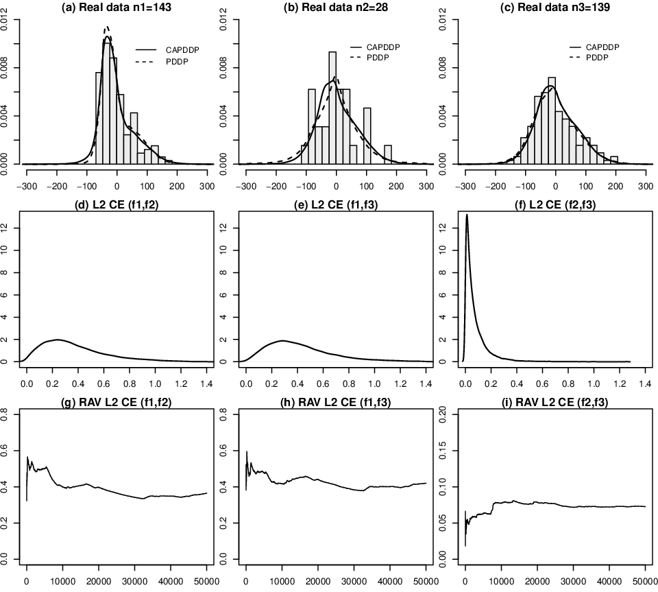
Real data example: The data set is to be found at and involves data from 312 individuals. We take the observation as SGOT (serum glutamic-oxaloacetic transaminase) level, just prior to liver transplant or death or the last observation recorded, under three conditions on the individual
- 1.
The individual is dead without transplantation.
- 2.
The individual had a transplant.
- 3.
The individual is alive without transplantation.
We normalize the means of all three data sets to zero. Since it is reasonable to assume the densities for the observations are similar for the three categories (especially for the last two), we adopt the model proposed in this paper with . The number of transplanted individuals is small (sample size of 28) so it is reasonable to borrow strength for this density from the other two. We took the hyperparameters of the Dirichlet priors for the mixing weights are for
We sample points from the predictives after a burn-in of .
The following results are presented in Figure 6:
- 1.
In (a)–(c).The histograms for the three data sets along with the superimposed predictive density curves of the -PDDP (solid) and -CAPDDP(dashed).
- 2.
In (d)–(f) the approximate densities of the sampled values of the conditonal expectations of the distances.
We note how the distribution of concentrates near zero, and the similarity of the distributions of and .
- 3.
In (g)–(i) the running averages.
General distinctive features between the CAPDDP and the PDDP models include:
- 1.
The average number of clusters during CAPDDP computations is larger than the average number of clusters in PDDP computations. A detailed comparison between the numerical approximations of the average number of clusters, for both the CAPDDP and the PDDP case, can be found in Table where we compare the average number of clusters coming from the three numerical examples.
- 2.
Borrowing of strength, seems to be sometimes weaker for the undersampled data set in the CAPDDP case. A detailed comparison on the borrowing of strength for the second predictiive in the three numerical examples can be found in Table . The larger the predictive running average for the selection probability is, the weaker the borrowing of strength between the second data set and the other two covariate data sets.
6. Discussion. We have shown when constructing pairwise dependent random densities, for the purposes of borrowing strength, the random Dirichlet processes used to effect this can be taken to have identical atoms. Random probability measures can be constructed by adapting the weights to these atoms and can provide arbitrary degrees of proximity; from identical to far apart. These distances can be readily evaluated precisely because they have identical atoms and hence share the same supports. Also the time complexity difference between the two algorithms is substancial. Let be the time complexity diffrerence between the PDDP and the CAPDDP algorithms based on a single sweep of the associated Gibbs samplers. Then it is not difficult to verify that
where is a Poisson random variable with mean and being the global minimum of the auxiliary variables ’s for and (Muliere, Tardella 1998). This time complexity difference is due to the fact that in the uncommon atom case we have to sample the posterior locations of different random measures.
We can also extend this principle to regression scenarios whereby densities are characterized by covariates . We can still adopt the idea of common atoms by designing
where
So as before we would have
and the covariate dependent weights will adapt the weights on the atoms to change the shape of the density. This could be densities which are far apart, based on a covariate pair which are far apart, or densities close to each other when the covariates are close. Indeed this is a simpler version of many Bayesian nonparametric regression models which typcially include in and have . We believe these extras are unnecessary.
To conform with our model described in Section 3 we could now take
with and for all . So, for each , for , is a stick-breaking set of weights, mutually independent over , and for each , is a Dirichlet process, mutually independent over .
This is not as complicated as it looks, essentially we would replace a finite with . So if covariates are from the set then we would model
Of course, in practice, only a finite number of covariates would be observed.
Acknowledgement. The work was completed during a visit by the third author to the University of the Aegean in Karlovassi, Samos.
| Data sets and sample sizes | Model | Predictive 1 | Predictive 2 | Predictive 3 |
|---|---|---|---|---|
| gamma-normal-gamma | CAPDDP | 3.075 | 4.456 | 4.044 |
| PDDP | 1.571 | 1.079 | 2.183 | |
| normal 3-mixtures | CAPDDP | 4.861 | 4.773 | 3.154 |
| PDDP | 3.090 | 3.041 | 3.062 | |
| real example | CAPDDP | 5.045 | 6.178 | 4.328 |
| PDDP | 3.090 | 3.041 | 3.062 |
| Data sets and sample sizes | Model | |||
|---|---|---|---|---|
| gamma-normal-gamma | CAPDDP | 0.343 | 0.301 | 0.356 |
| PDDP | 0.484 | 0.167 | 0.349 | |
| normal 3-mixtures | CAPDDP | 0.146 | 0.702 | 0.152 |
| PDDP | 0.359 | 0.405 | 0.236 | |
| real example | CAPDDP | 0.341 | 0.325 | 0.334 |
| PDDP | 0.305 | 0.328 | 0.366 |
References.
-
Bulla, P., Muliere, P. and Walker, S.G. (2009). A Bayesian nonparametric estimator of a multivariate survival function. Journal of Statistical Planning and Inference 139, 3639–3648.
-
De Iorio, M., Müller, P., Rosner, G.L. and MacEachern, S.N. (2004). An ANOVA model for dependent random measures. Journal of the American Statistical Association 99, 205–215.
-
Dunson, D.B. and Park, J.H. (2008). Kernel stick-breaking processes. Biometrika 95, 307–323.
-
Ferguson, T.S. (1973). A Bayesian analysis of some nonparametric problems. Annals of Statistics 1, 209-230.
-
Griffin, J.E. and Steel, M.F.J. (2006). Order-based dependent Dirichlet processes. Journal of the American Statistical Association 101, 179–194.
-
Griffin, J.E., Kolossiatis, M. and Steel, M.F.J. (2013). Comparing distributions by using dependent normalized random-measure mixtures. Journal of the Royal Statistical Society, Series B 75, 499–529.
-
Hatjispyros, S.J., Nicoleris, T. and Walker, S.G. (2011). Dependent mixtures of Dirichlet processes. Computational Statistics and Data Analysis 55, 2011–2025.
-
Hjort, N.L., Holmes, C.C., Müller, P. and Walker, S.G. (2010). Bayesian Nonparametrics. Cambridge University Press.
-
Ishwaran, H. and James, L.F. (2001). Gibbs sampling methods for stick-breaking priors. Journal of the American Statistical Association 96, 161–173.
-
Kalli, M., Griffin, J.E. and Walker, S.G. (2010). Slice Sampling Mixture Models. Statistics and Computing 21, 93–105.
-
Kolossiatis, M., Griffin, J.E. and Steel, M.F.J. (2013). On Bayesian nonparametric modelling of two correlated distributions. Statistics and Computing 23, 1–15.
-
Lo, A.Y. (1984). On a class of Bayesian nonparametric estimates I. Density estimates. Annals of Statistics 12, 351–357.
-
MacEachern, S.N. (1999). Dependent nonparametric processes. In “Proceedings of the Section on Bayesian Statistical Science”, pp. 50–55. American Statistical Association.
-
Muliere, P., Tardella, L. (1998). Approximating distributions of random functionals of Ferguson-Dirichlet priors. Canadian Journal of Statistics 26, 283–297.
-
Müller, P., Quintana, F. and Rosner, G. (2004). A method for combining inference across related nonparametric Bayesian models. Journal of the Royal Statistical Society, Series B 66, 735–749.
-
Sethuraman, J. (1994). A constructive definition of Dirichlet priors. Statistica Sinica 4, 639–650.
-
Walker, S.G. (2007). Sampling the Dirichlet mixture model with slices. Communications in Statistics 36, 45–54.


Abstract
The paper is concerned with constructing pairwise dependence between random density functions each of which is modeled as a mixture of Dirichlet process model. The key to this is how to create dependencies between random Dirichlet processes. The present paper adopts a plan previously used for creating pairwise dependence, with the simplification that all random Dirichlet processes share the same atoms. Our contention is that for all dependent Dirichlet process models, common atoms are sufficient.
We show that by adopting common atoms, it is possible to compute the distances between all pairs of random probability measures.
Keywords: Bayesian nonparametric inference; Dependent Dirichlet process; distance; Mixture of Dirichlet process; Pairwise dependence.