Convergence of Tikhonov regularization for solving ill-posed operator equations with solutions defined on surfaces

Guozhi Dong Note: Computational Science Center, University of Vienna, Oskar-Morgenstern Platz 1, 1090 Vienna, Austria (guozhi.dong@univie.ac.at) Bert Jüttler Note: Institute of Applied Geometry, Johannes Kepler University of Linz, Altenberger Str. 69, A-4040 Linz, Austria (bert.juettler@jku.at) Otmar Scherzer Note: Computational Science Center, University of Vienna, Oskar-Morgenstern Platz 1, 1090 Vienna, and Johann Radon Institute for Computational and Applied Mathematics (RICAM), Austrian Academy of Sciences, Altenberger Str. 69, A-4040 Linz, Austria (otmar.scherzer@univie.ac.at) Thomas Takacs Note: Institute of Applied Geometry, Johannes Kepler University of Linz, Altenberger Str. 69, A-4040 Linz, Austria (thomas.takacs@jku.at)

Abstract

We study Tikhonov regularization for solving ill–posed operator equations where the solutions are functions defined on surfaces. One contribution of this paper is an error analysis of Tikhonov regularization which takes into account perturbations of the surfaces, in particular when the surfaces are approximated by spline surfaces. Another contribution is that we highlight the analysis of regularization for functions with range in vector bundles over surfaces. We also present some practical applications, such as an inverse problem of gravimetry and an imaging problem for denoising vector fields on surfaces, and show the numerical verification.

1 Introduction

We are interested in solving linear inverse problems

F\mathbf{u}=\mathbf{y},

(1.1)

where $F:{\mathcal{U}}_{1}\to{\mathcal{U}}_{2}$ is a bounded operator between Hilbert spaces of functions defined on surfaces. Note that the functions in spaces ${\mathcal{U}}_{1}$ and ${\mathcal{U}}_{2}$ might be defined on different surfaces ${\mathcal{M}}_{1}$ and ${\mathcal{M}}_{2}$ respectively. Especially we pay attention to applications (see also Section 3 and 4) where ${\mathcal{U}}_{1}$ denotes a space of functions from a surface ${\mathcal{M}}_{1}$ into the vector bundle or into the tangent vector bundle.

We assume that solving (1.1) is ill–posed and requires some regularization to approximate the solution in a stable way. The regularization method of choice for solving (1.1) is Tikhonov regularization, which consists in approximating a solution of (1.1) by a minimizer of the functional

\mathcal{T}_{\alpha,\mathbf{y}^{\delta}}(\mathbf{u}):=\left\|F\mathbf{u}-\mathbf{y}^{\delta}\right\|_{{\mathcal{U}}_{2}}^{2}+\alpha\mathcal{R}(\mathbf{u})

(1.2)

over ${\mathcal{U}}_{1}$ . Here $\mathbf{y}^{\delta}$ denotes some approximation of the exact data $\mathbf{y}$ , from which we assume that

\left\|\mathbf{y}-\mathbf{y}^{\delta}\right\|_{{\mathcal{U}}_{2}}\leq\delta.

(1.3)

Moreover, $\alpha>0$ is a regularization parameter, and $\mathcal{R}$ is an appropriate regularization functional. In contrast to previous work [3, 4, 9, 11, 14, 15, 22, 27] we are emphasizing on Hilbert spaces of functions defined on surfaces.

The analysis of Tikhonov regularization has advanced from a theory for solving ill–posed operator equations in a Hilbert space setting, both in a finite and an infinite dimensional setting (see for instance [2, 3, 4, 14, 23]), to more complex situations, when $F$ is nonlinear [8, 9, 11, 15] or with sophisticated regularization [17, 19, 20, 22, 24, 27, 26], and in statistical setting [18]. The analysis of finite dimensional approximations of regularizers in infinite dimensional spaces (see for instance [5, 24, 30]) is highly relevant for this work. The results of [24] are already quite general, but do not cover approximations of solutions of (1.1) by functions defined on approximating surfaces. Note that for functions defined on subsets of an Euclidean space, the finite dimensional functions approximating infinite dimensional functions are also defined on the Euclidean space, and this is not the case anymore if the underlying manifold is approximated. In this paper the differential geometrical concept of a pullback is used to compare functions defined on different surfaces.

The second issue of this paper is, that the solution of (1.1) may be a function with range in a vector bundle. Consequently, when the surface is approximated also the vector bundle, or in other words, the range of the function is varying by approximation. To resolve this issue we consider vector fields represented with ambient bases. It is then presented in the paper that the analysis of regularization for vector fields on surfaces can be incorporated into a general framework developed for vector valued functions on surfaces.

We consider several applications and perform numerical tests. One example concerns reconstructing the magnetization from measurements of the magnetic potential [10, 25, 31]. Another numerical test example concerns vector field denoising. Our analysis on regularizing tangent vector fields in ambient spaces provides a different point of view to existing work on tangent vector field regularization (see for instance [21, 28, 29]).

The paper is organized as follows: In Section 2 we first review standard regularization results in an infinite dimensional setting, and then perform a convergence analysis of Tikhonov regularization taking into account approximated surfaces, which cannot be handled with the existing theory. In Section 3, we introduce proper spaces for functions with range in vector bundles, and discuss applications of the regularization theory for recovering vector fields in ambient spaces. We make an additional discussion on recovering tangent vector fields there. Finally, in Section 4, we present some examples and verify the theoretical results numerically. The underlying geometric concepts, including all the basic notations, are summarized in the Appendix A.

2 Regularization for functions defined on surfaces

Below we first review results from the regularization literature (see [3, 11, 22]), which provide well-posedness, convergence and stability of Tikhonov regularization. For this purpose we summarize the basic assumptions needed throughout this paper.

Assumption 2.1 (Chapter 3, [22]).

In the context of Tikhonov regularization (1.2) we make the following assumptions:

1.

Let ${\mathcal{U}}_{1}$ , ${\mathcal{U}}_{2}$ be two Hilbert spaces.
2.

$F:\mathcal{D}(F)\subseteq{\mathcal{U}}_{1}\to{\mathcal{U}}_{2}$ is a bounded linear operator with domain $\mathcal{D}(F)$ , which is weakly sequentially closed.
3.

$\mathcal{R}:{\mathcal{U}}_{1}\to[0,\infty]$ is a proper, convex, and sequentially weakly lower-semi continuous functional satisfying $\mathcal{D}:=\mathcal{D}(\mathcal{R})\cap\mathcal{D}(F)\neq\emptyset.$
4.

For every $\alpha,\theta>0$ the sets $M_{\alpha,\mathbf{y}}(\theta):=\left\{\mathbf{u}\in{\mathcal{U}}_{1}:\mathcal{T}_{\alpha,\mathbf{y}}(\mathbf{u})\leq\theta\right\}$ are weakly sequentially compact.

2.1 Standard regularization theory

We review some regularization results from the literature:

Theorem 2.2 (Chapter 3, [22]).

Let $F$ , $\mathcal{R}$ , $\mathcal{D}$ , ${\mathcal{U}}_{1}$ and ${\mathcal{U}}_{2}$ satisfy Assumption 2.1, and $\mathbf{y}$ and $\mathbf{y}^{\delta}$ satisfy (1.3).

•

Assume that $\alpha>0$ . Then there exists a minimizer of $\mathcal{T}_{\alpha,\mathbf{y}^{\delta}}$ . If $(\mathbf{y}_{k})_{k\in\mathbb{N}}$ is a sequence converging to $\mathbf{y}$ in ${\mathcal{U}}_{2}$ , then every sequence

\left(\mathbf{u}_{k}:=\mathrm{\,arg\,min}\left\{\mathcal{T}_{\alpha,\mathbf{y}_{k}}(\mathbf{u}):\mathbf{u}\in\mathcal{D}\right\}\right)_{k\in\mathbb{N}}

has a weakly convergent subsequence in ${\mathcal{U}}_{1}$ , and the limit is a minimizer of $\mathcal{T}_{\alpha,\mathbf{y}}$ .

•

If there exists $\mathbf{u}_{0}\in\mathcal{D}$ such that

$F\mathbf{u}_{0}=\mathbf{y}.$ (2.1)

Then there exists an $\mathcal{R}$ minimizing solution $\mathbf{u}^{\dagger}$ . That is

$\mathcal{R}(\mathbf{u}^{\dagger})=\min\left\{\mathcal{R}(\mathbf{u}):\mathbf{u}\in\mathcal{D},F\mathbf{u}=\mathbf{y}\right\}.$
•

Assume that $\alpha=\alpha(\delta):(0,\infty)\to(0,\infty)$ satisfies

$\alpha\to 0,\;\frac{\delta^{2}}{\alpha}\to 0,\text{ as }\delta\to 0.$ (2.2)

Let $(\mathbf{y}_{k})_{k\in\mathbb{N}}$ satisfy $\left\|\mathbf{y}-\mathbf{y}_{k}\right\|_{{\mathcal{U}}_{2}}\leq\delta_{k}$ and set $\alpha_{k}=\alpha(\delta_{k})$ . Then every sequence $(\mathbf{u}_{k}=\text{argmin}\left\{\mathcal{T}_{\alpha_{k},\mathbf{y}_{k}}(\mathbf{u}):\mathbf{u}\in\mathcal{D}\right\})$ has a weakly convergent subsequence, and the limit is an $\mathcal{R}$ -minimizing solution.

•

Moreover, if in addition $\mathbf{u}^{\dagger}$ satisfies a source condition, which assumes that there exists an element $W\in{\mathcal{U}}_{2}$ , such that

$F^{*}W\in\partial\mathcal{R}(\mathbf{u}^{\dagger}).$ (2.3)

Here $\partial\mathcal{R}(\mathbf{u}^{\dagger})$ denotes the subgradient of $\mathcal{R}$ at $\mathbf{u}^{\dagger}$ , and $F^{*}:{\mathcal{U}}_{2}\to{\mathcal{U}}_{1}$ is the adjoint operator of $F$ .

Then, the $\mathcal{R}$ -minimizing solution satisfies

B_{\mathcal{R}}(\mathbf{u}_{k},\mathbf{u}^{\dagger})=\mathcal{O}\left(\max\left\{\frac{\delta_{k}^{2}}{\alpha_{k}},\alpha_{k}\right\}\right),

where $B_{\mathcal{R}}(\cdot,\cdot)$ denotes the Bregman distance with respect to the convex functional $\mathcal{R}$ , see for instance [17].

2.2 Convergence analysis taking into account surface perturbations

In the following we study Tikhonov regularization, consisting in minimizing the functional $\mathcal{T}_{\alpha,\mathbf{y}^{\delta}}$ in (1.2), where $F:{\mathcal{U}}_{1}\to{\mathcal{U}}_{2}$ is an operator between function spaces

{\mathcal{U}}_{i}:=\mathcal{X}_{i}({\mathcal{M}}_{i}):=\left\{{\mathbf{x}}_{i}:{\mathcal{M}}_{i}\rightarrow\mathbb{R}^{r_{i}}\right\},\text{ for }r_{i}\in\mathbb{N}^{+},\;\text{ and }i=1,2,

of functions defined on surfaces ${\mathcal{M}}_{i}$ , $i=1,2$ , respectively. We consider families of surfaces $\left\{{\mathcal{M}}_{i,\sigma}\right\}_{\sigma>0}$ approximating the surfaces ${\mathcal{M}}_{i,0}:={\mathcal{M}}_{i}$ , $i=1,2$ . In what follows we use the following abbreviations:

{\mathcal{U}}_{i,\sigma}:=\mathcal{X}_{i}({\mathcal{M}}_{i,\sigma})\,,\quad\left\|\cdot\right\|_{i,\sigma}:=\left\|\cdot\right\|_{{\mathcal{U}}_{i,\sigma}}\,,\quad i=1,2,\;\sigma>0\,,

(2.4)

where we delete the superscript $0$ in case $\sigma=0$ . That is $\left\|\cdot\right\|_{1}=\left\|\cdot\right\|_{1,0}$ . We need a few assumptions on the approximating surfaces.

Assumption 2.3.

Let $\left\{{\mathcal{M}}_{i,\sigma}\right\}_{\sigma>0}$ be a sequence of surfaces approximating the surfaces ${\mathcal{M}}_{i}$ for $i=1,2$ , then we assume the following properties and estimates hold:

•

For every $i=1,2$ and every $\sigma\geq 0$ , every surface ${\mathcal{M}}_{i,\sigma}$ can be parametrized by a patch

$m_{i,\sigma}:\Omega_{i}\subset\mathbb{R}^{d_{i}}\to{\mathcal{M}}_{i,\sigma}\subset\mathbb{R}^{d_{i}+1}\,,\quad\sigma\geq 0,$

with the same parameter domain $\Omega_{i}$ , and $m_{i,\sigma}$ is a bijection.

•

The operators

	$\displaystyle T_{i,\sigma}:{\mathcal{U}}_{i}$	$\displaystyle\to{\mathcal{U}}_{i,\sigma}$		(2.5)
	$\displaystyle{\mathbf{x}}_{i}$	$\displaystyle\mapsto{\mathbf{x}}_{i}\circ m_{i}\circ(m_{i,\sigma})^{-1}$		(2.5)

and the inverse

	$\displaystyle(T_{i,\sigma})^{-1}:{\mathcal{U}}_{i,\sigma}$	$\displaystyle\to{\mathcal{U}}_{i}$		(2.6)
	$\displaystyle{\mathbf{x}}_{i,}{{}_{\sigma}}$	$\displaystyle\mapsto{\mathbf{x}}_{i,}{{}_{\sigma}}\circ m_{i,\sigma}\circ m_{i}^{-1}$		(2.6)

are uniformly bounded. Here by bounded we mean that there exists a real constant $C$ such that

\left\|T_{i,\sigma}{\mathbf{x}}_{i}\right\|_{i,\sigma}\leq C\left\|{\mathbf{x}}_{i}\right\|_{i}\;\text{ and }\left\|(T_{i,\sigma})^{-1}{\mathbf{x}}_{i,}{{}_{\sigma}}\right\|_{i}\leq C\left\|{\mathbf{x}}_{i,}{{}_{\sigma}}\right\|_{i,\sigma}.

(2.7)

•

Let the family of operators $F_{\sigma}:{\mathcal{U}}_{1,}{{}_{\sigma}}\to{\mathcal{U}}_{2,}{{}_{\sigma}}$ , $\sigma>0$ and the operator $F:{\mathcal{U}}_{1}\to{\mathcal{U}}_{2}$ satisfy

$\rho(\sigma):=\left\|(T_{2,\sigma})^{-1}F_{\sigma}T_{1,\sigma}-F\right\|\to 0\text{ for }\sigma\to 0.$ (2.8)
•

Let $\mathcal{R}_{\sigma}:{\mathcal{U}}_{1,}{{}_{\sigma}}\rightarrow[0,\infty]$ with $\sigma>0$ be the family of regularization functionals, then there exists $C_{M}\in\mathbb{R}$ such that

$\left|\mathcal{R}_{\sigma}(T_{1,\sigma}\mathbf{u})-\mathcal{R}(\mathbf{u})\right|\leq C_{M}\gamma_{1}(\sigma),$ (2.9)

holds uniformly for all $\mathbf{u}\in A_{M}\subset{\mathcal{U}}_{1}$ , with $A_{M}:=\left\{{\mathbf{x}}_{1}\in{\mathcal{U}}_{1}:\mathcal{R}({\mathbf{x}}_{1})\leq M\right\}.$
•

There exists an $\mathcal{R}$ -minimizing solution $\mathbf{u}^{\dagger}$ of (1.1).

•

$\mathbf{y}_{\sigma},\mathbf{y}_{\sigma}^{\delta}\in{\mathcal{U}}_{2,}{{}_{\sigma}}$ satisfy

\left\|\mathbf{y}_{\sigma}-\mathbf{y}_{\sigma}^{\delta}\right\|_{2,\sigma}=\mathcal{O}(\delta)\,\text{ and }\left\|(T_{2,\sigma})^{-1}\mathbf{y}_{\sigma}-\mathbf{y}\right\|_{2}=\mathcal{O}(\gamma_{2}(\sigma))\,,

(2.10)

where $\gamma_{2}(\sigma)\to 0$ for $\sigma\to 0$ .

Remark 2.4 (On Assumption 2.3).

For surfaces which can not be parametrized by a single domain (such as a sphere), we assume that the domain can be covered by patches, and the above assumption has to be satisfied on every patch.

Remark 2.5.

(1.3), (2.7) and (2.10) actually implies that

\max\left\{\left\|(T_{2,\sigma})^{-1}\mathbf{y}_{\sigma}^{\delta}-\mathbf{y}\right\|_{2},\left\|\mathbf{y}_{\sigma}^{\delta}-(T_{2,\sigma})\mathbf{y}\right\|_{2,\sigma}\right\}=\mathcal{O}(\gamma_{2}(\sigma)+\delta).

(2.11)

For given data $\mathbf{y}_{\sigma}^{\delta}$ we consider the regularization strategy consisting in minimization of the Tikhonov functional for $\mathbf{u}_{\sigma}\in{\mathcal{U}}_{1,}{{}_{\sigma}}$ ,

\mathcal{T}_{\alpha,\sigma,\mathbf{y}_{\sigma}^{\delta}}(\mathbf{u}_{\sigma}):=\left\|F_{\sigma}\mathbf{u}_{\sigma}-\mathbf{y}_{\sigma}^{\delta}\right\|_{2,\sigma}^{2}+\alpha\mathcal{R}_{\sigma}(\mathbf{u}_{\sigma}).

(2.12)

Theorem 2.6.

Let the Assumptions 2.1, 2.3 hold. Moreover, assume that $\alpha:=\alpha(\sigma,\delta)\to 0$ for $\sigma\to 0$ , and $\delta\to 0$ and that

\frac{\rho^{2}}{\alpha}\to 0,\;\frac{\gamma_{2}^{2}}{\alpha}\to 0,\;\frac{\delta^{2}}{\alpha}\to 0\text{ and }\gamma_{1}\to 0,\text{ for }\sigma,\delta\;\to 0.

(2.13)

Let $(\mathbf{u}_{k}:=\mathbf{u}_{\alpha_{k},\sigma_{k},\delta_{k}})$ be a sequence of minimizers of $\mathcal{T}_{k}:=\mathcal{T}_{\alpha_{k},\sigma_{k},\mathbf{y}_{k}}$ , defined in (2.12), with $\mathbf{y}_{k}:=\mathbf{y}_{\sigma_{k}}^{\delta_{k}}$ satisfying (2.10). In addition we denote by

\check{\mathbf{u}}_{k}=T_{1,k}^{-1}\mathbf{u}_{k}\in{\mathcal{U}}_{1}

(2.14)

the pullback of $\mathbf{u}_{k}$ onto ${\mathcal{M}}_{1}$ , and $T_{i,k}:=T_{i,\sigma_{k}}$ for $i=1,2$ and $k\in\mathbb{N}.$

•

We use the abbreviations $\rho_{k}:=\rho(\sigma_{k})$ , $\gamma_{i,k}:=\gamma_{i}(\sigma_{k})$ for $i=1,2$ and $\alpha_{k}:=\alpha(\sigma_{k},\delta_{k})$ . Then the limit of every convergent subsequence of $(\check{\mathbf{u}}_{k})$ is an $\mathcal{R}$ -minimizing solution.

•

Moreover, assuming the source condition (2.3) holds, then, the $\mathcal{R}$ -minimizing solution has the convergence rate by Bregman-distance

B_{\mathcal{R}}(\check{\mathbf{u}}_{k},\mathbf{u}^{\dagger})=\mathcal{O}\left(\max\left\{\frac{\rho_{k}^{2}}{\alpha_{k}},\frac{\gamma_{2,k}^{2}}{\alpha_{k}},\frac{\delta_{k}^{2}}{\alpha_{k}},\gamma_{1,k}\right\}\right).

Proof.

•

To prove the first item let $\mathbf{u}_{k}$ denote the minimizer of $\mathcal{T}_{k}$ . Moreover, we use the abbreviations $F_{k}=F_{\sigma_{k}}$ , $\mathcal{R}_{k}=\mathcal{R}_{\sigma_{k}}$ , and $\mathbf{u}^{\dagger}_{k}=T_{1,k}\mathbf{u}^{\dagger}$ .

Then, according to the definition of a minimizer, we have (2.15)

\left\|F_{k}\mathbf{u}_{k}-\mathbf{y}_{k}\right\|_{2,k}^{2}+\alpha_{k}\mathcal{R}_{k}(\mathbf{u}_{k})\leq\left\|F_{k}\mathbf{u}^{\dagger}_{k}-\mathbf{y}_{k}\right\|_{2,k}^{2}+\alpha_{k}\mathcal{R}_{k}(\mathbf{u}^{\dagger}_{k}).

(2.15)

Since the vector field $\mathbf{u}^{\dagger}$ solves $F\mathbf{u}^{\dagger}=\mathbf{y}$ , and (2.5) in Assumption 2.3 and Equations (2.8), (2.11) hold, it follows that

$\displaystyle\left\\|F_{k}\mathbf{u}^{\dagger}_{k}-\mathbf{y}_{k}\right\\|_{2,k}^{2}$	$\displaystyle=\left\\|T_{2,k}T_{2,k}^{-1}(F_{k}\mathbf{u}^{\dagger}_{k}-\mathbf{y}_{k})\right\\|_{2,k}^{2}$	(2.16)
	$\displaystyle\leq C\left\\|T_{2,k}^{-1}(F_{k}\mathbf{u}^{\dagger}_{k}-\mathbf{y}_{k})\right\\|_{2}^{2}$
	$\displaystyle=C\left\\|T_{2,k}^{-1}F_{k}T_{1,k}\mathbf{u}^{\dagger}-F\mathbf{u}^{\dagger}+\mathbf{y}-T_{2,k}^{-1}\mathbf{y}_{k}\right\\|_{2}^{2}$
	$\displaystyle=\mathcal{O}(\rho_{k}^{2}+\gamma_{2,k}^{2}+\delta_{k}^{2}),$

Applying (2.9), we find

\displaystyle\biggl|\mathcal{R}_{k}(\mathbf{u}^{\dagger}_{k})-\mathcal{R}(\mathbf{u}^{\dagger})\biggr|

\displaystyle=\mathcal{O}(\gamma_{1,k}).

(2.17)

Using the estimates (2.16) and (2.17) in (2.15) shows that

		$\displaystyle\left\\|F_{k}\mathbf{u}_{k}-\mathbf{y}_{k}\right\\|_{2,k}^{2}+\alpha_{k}\left\|\mathcal{R}_{k}(\mathbf{u}_{k})-\mathcal{R}(\mathbf{u}^{\dagger})\right\|$		(2.18)
	$\displaystyle=$	$\displaystyle\mathcal{O}\left(\max\left\{\rho_{k}^{2},\gamma_{2,k}^{2},\delta_{k}^{2},\alpha_{k}\gamma_{1,k}\right\}\right).$		(2.18)

From (2.13) and (2.18) it follows that $\left\{\mathcal{R}_{k}(\mathbf{u}_{k}):k\in\mathbb{N}\right\}$ is uniformly bounded, and consequently it follows from (2.9) that

\biggl|\mathcal{R}(\check{\mathbf{u}}_{k})-\mathcal{R}_{k}(\mathbf{u}_{k})\biggr|=\mathcal{O}(\gamma_{1,k}).

(2.19)

Since $\check{\mathbf{u}}_{k}:=T_{1,k}^{-1}\mathbf{u}_{k}$ , it follows from (2.6), (2.7), (2.18) and (2.19) that

	$\displaystyle\left\\|T_{2,k}^{-1}F_{k}T_{1,k}\check{\mathbf{u}}_{k}-T_{2,k}^{-1}\mathbf{y}_{k}\right\\|_{2}^{2}+\alpha_{k}\left(\mathcal{R}(\check{\mathbf{u}}_{k})-\mathcal{R}(\mathbf{u}^{\dagger})\right)$	(2.20)
$\displaystyle\leq$	$\displaystyle C\left(\left\\|F_{k}\mathbf{u}_{k}-\mathbf{y}_{k}\right\\|_{2,k}^{2}\right)+\alpha_{k}\biggl\|\mathcal{R}_{k}(\mathbf{u}_{k})-\mathcal{R}(\mathbf{u}^{\dagger})\biggr\|+\alpha_{k}\biggl\|\mathcal{R}(\check{\mathbf{u}}_{k})-\mathcal{R}_{k}(\mathbf{u}_{k})\biggr\|$
$\displaystyle\leq$	$\displaystyle(1+C)\left(\left\\|F_{k}\mathbf{u}_{k}-\mathbf{y}_{k}\right\\|_{2,k}^{2}+\alpha_{k}\biggl\|\mathcal{R}_{k}(\mathbf{u}_{k})-\mathcal{R}(\mathbf{u}^{\dagger})\biggr\|\right)+\alpha_{k}\biggl\|\mathcal{R}(\check{\mathbf{u}}_{k})-\mathcal{R}_{k}(\mathbf{u}_{k})\biggr\|$
$\displaystyle=$	$\displaystyle\mathcal{O}\left(\max\left\{\rho_{k}^{2},\gamma_{2,k}^{2},\delta_{k}^{2},\alpha_{k}\gamma_{1,k}\right\}\right).$

From the assumptions on the parameters (2.13) it follows after division of the inequality by $\alpha_{k}$ and taking the limit $k\to\infty$ afterwards that

\limsup_{k}\mathcal{R}(\check{\mathbf{u}}_{k})\leq\mathcal{R}(\mathbf{u}^{\dagger}),

and consequently also

\lim_{k}\left\|T_{2,k}^{-1}F_{k}T_{1,k}\check{\mathbf{u}}_{k}-T_{2,k}^{-1}\mathbf{y}_{k}\right\|_{2}^{2}=0.

(2.21)

It follows then from (2.21) and (2.8) that $\left\|F\check{\mathbf{u}}_{k}\right\|$ is uniformly bounded.

Similarly as in [22, Theorem 3.26] it can be seen that for some fixed $\alpha_{0}$ , there is $N_{0}\in\mathbb{N}^{+}$ the set $\left\{\mathcal{T}_{\alpha_{0},\mathbf{y}}(\check{\mathbf{u}}_{k}):k\geq N_{0}\right\}$ is uniformly bounded. Then by the weak sequential compactness of the level sets of $\mathcal{T}_{\alpha_{0},\mathbf{y}}$ (Assumption 2.1), we have $\left\{\check{\mathbf{u}}_{k}\right\}$ is bounded in ${\mathcal{U}}_{1}$ . Thus there is a weakly convergent subsequence of $\left\{\check{\mathbf{u}}_{k}\right\}$ , for which we denote the weak limit by $\bar{\mathbf{u}}\in{\mathcal{U}}_{1}$ .

Using (2.21) it follows that

		$\displaystyle\left\\|F\bar{\mathbf{u}}-\mathbf{y}\right\\|_{2}^{2}$
	$\displaystyle=$	$\displaystyle\left\\|F\bar{\mathbf{u}}-T_{2,k}^{-1}F_{k}T_{1,k}\bar{\mathbf{u}}+T_{2,k}^{-1}F_{k}T_{1,k}\bar{\mathbf{u}}-T_{2,k}^{-1}\mathbf{y}_{k}+T_{2,k}^{-1}\mathbf{y}_{k}-\mathbf{y}\right\\|_{2}^{2}\to 0\,.$

This in particular shows that $\bar{\mathbf{u}}\in{\mathcal{U}}_{1}$ solves (1.1). The weakly lower semi-continuity of the functional $\mathcal{R}(\cdot)$ implies that

\mathcal{R}(\bar{\mathbf{u}})\leq\liminf_{k}\mathcal{R}(\check{\mathbf{u}}_{k})\leq\limsup_{k}\mathcal{R}(\check{\mathbf{u}}_{k})\leq\mathcal{R}(\mathbf{u}^{\dagger}),

which because $\mathbf{u}^{\dagger}$ is an $\mathcal{R}$ - minimizing solution tells us that $\mathcal{R}(\bar{\mathbf{u}})=\mathcal{R}(\mathbf{u}^{\dagger})$ , and thus $\bar{\mathbf{u}}$ is also an $\mathcal{R}$ - minimizing solution of (1.1).

•

To prove the convergence rate result we reconsider (2.20) and the family of operators $\{T_{2,k}^{-1}F_{k}T_{1,k}:k\in\mathbb{N}\}$ . Using (2.8) in Assumption 2.3, it follows that

\left\|T_{2,k}^{-1}F_{k}T_{1,k}-F\right\|=\mathcal{O}\left(\rho_{k}\right).

Moreover, from (2.11) it follows that

\left\|T_{2,k}^{-1}\mathbf{y}_{k}-\mathbf{y}\right\|_{2}=\mathcal{O}(\gamma_{2,k}+\delta_{k}).

We can apply the results of [24, Theorem 2.6] with the triangle inequality to taking care of some additional error terms on the right side of (2.20), then we get

B_{\mathcal{R}}(\check{\mathbf{u}}_{k},\mathbf{u}^{\dagger})=\mathcal{O}\left(\max\left\{\frac{\rho_{k}^{2}}{\alpha_{k}},\frac{\gamma_{2,k}^{2}}{\alpha_{k}},\frac{\delta_{k}^{2}}{\alpha_{k}},\gamma_{1,k}\right\}\right).

∎

Remark 2.7.

We note that if the parameters are chosen in the following way, $\rho(\sigma)=\mathcal{O}(\gamma_{1}(\sigma))=\mathcal{O}(\gamma_{2}(\sigma))=\mathcal{O}(\delta)$ (for instance by appropriate discretization) and $\alpha(\sigma,\delta)=\mathcal{O}(\delta)$ , then we derive the standard convergence rates

B_{\mathcal{R}}(\check{\mathbf{u}}_{k},\mathbf{u}^{\dagger})=\mathcal{O}\left(\delta_{k}\right).

Especially, if we choose $\mathcal{R}(\cdot)=\left\|\cdot\right\|_{1}^{2},$ then we have

B_{\mathcal{R}}(\check{\mathbf{u}}_{k},\mathbf{u}^{\dagger})=\left\|\check{\mathbf{u}}_{k}-\mathbf{u}^{\dagger}\right\|_{1}^{2}=\mathcal{O}\left(\delta_{k}\right).

Theorem 2.6 is a generalization of Theorem 2.2. Actually Theorem 2.2 is a trivial case of Theorem 2.6 when $\sigma\equiv 0$ .

In the following, we shortly discuss a case example in which ${\mathcal{U}}_{i}\;(i=1,2)$ are the Sobolev spaces on surfaces (see [16] for instance).

Example 2.8.

Let ${\mathcal{U}}_{i,}{{}_{\sigma}}:=W^{k_{i},2}({\mathcal{M}}_{i,\sigma},\mathbb{R}^{r_{i}})$ , for $i=1,2$ , $k_{i}\in\mathbb{N}$ and $r_{i}\in\mathbb{R}^{+}$ ,

m_{i,\sigma}\in W^{k_{i},\infty}(\Omega_{i},{\mathcal{M}}_{i,\sigma})\;\text{ and }\;m_{i,\sigma}^{-1}\in W^{k_{i},\infty}({\mathcal{M}}_{i,\sigma},\Omega_{i}).

(2.22)

We have $T_{i,\sigma}$ and $T_{i,\sigma}^{-1}$ are bounded. Moreover, let

\gamma_{i}(\sigma):=\left\|m_{i,\sigma}-m_{i}\right\|_{W^{k_{i},\infty}(\Omega_{i})}\;

(2.23)

and assume that $\gamma_{i}:\mathbb{R}^{+}\to\mathbb{R}$ is uniformly bounded, monotonically increasing, and satisfies the convergence $\gamma_{i}(\sigma)\to 0$ as $\sigma\to 0$ . For a general operator equation (1.1) of which the data satisfies (1.3), we consider its Tikhonov regularization approximation (1.2) with $\mathcal{R}(\cdot)=\left\|\cdot\right\|_{{\mathcal{U}}_{1}}^{2}$ . Then (2.7), (2.9) and (2.10) are also fulfilled.

Remark 2.9.

In particular if $k_{i}=2$ and $m_{i,\sigma}$ is a uniform cubic spline approximation with grid size $h<1$ of $m_{i}$ which is $C^{2}$ -smooth, then the condition (2.22) holds and the estimate (2.23) can have an explicitly form, see for instance [1], that is

\gamma_{i}(h):=\left\|m_{i,h}-m_{i}\right\|_{W^{2,\infty}(\Omega_{i})}=\mathcal{O}(h)\;.

(2.24)

Remark 2.10.

Note the condition (2.8) has to be further checked for individual operators $F$ and $F_{\sigma}$ . The source condition (2.3) may require more smoothness on the non-disturbed surfaces ${\mathcal{M}}_{1}$ and ${\mathcal{M}}_{2}$ . For example: if $F:W^{1,2}({\mathcal{M}}_{1})\rightarrow L^{2}({\mathcal{M}}_{1})$ is the embedding operator, and $\mathcal{R}(\cdot)=\left|\cdot\right|_{W^{1,2}({\mathcal{M}}_{1})}$ , then condition (2.3) reads as

\Delta_{{\mathcal{M}}}\mathbf{u}^{\dagger}\in L^{2}({\mathcal{M}}_{1}),

where $\Delta_{{\mathcal{M}}}$ denotes the Laplace–Beltrami operator. It asks that $m_{1}\in W^{2,\infty}(\Omega_{1})$ , which is $one$ order higher regularity than $W^{1,\infty}(\Omega_{1})$ given in (2.22).

3 Application to recover vector fields in ambient spaces

In this section, we are studying an ill-posed operator equation, of which the solution is a functions with range in the vector bundle over a surface. A typical case is like a tangent vector field $\widetilde{\mathbf{u}}:{\mathcal{M}}\rightarrow\mathcal{T}{\mathcal{M}}$ (see Appendix A). As a consequence, in case of surface perturbations, also the range of the function $\widetilde{\mathbf{u}}$ is perturbed and we get the approximation

\widetilde{\mathbf{u}_{\sigma}}:{\mathcal{M}}_{\sigma}\rightarrow\mathcal{T}{\mathcal{M}}_{\sigma}.

To take this into account we consider vector fields represented by the basis in ambient space $\mathbb{R}^{d+1}$ of the surface ${\mathcal{M}}$ , which consist of vector valued functions $\mathbf{u}:{\mathcal{M}}\rightarrow\mathbb{R}^{d+1}$ .

We start by introducing some appropriate function spaces. The relevant geometric notations are summarized in Table 2 from the Appendix A.

3.1 Spaces of functions with range in the vector bundle

Before introducing the function spaces we outline a basic assumption first:

Assumption 3.1.

Let ${\mathcal{M}}\in\mathbb{R}^{d+1}$ be a $d$ -dimensional, differentiable surface, such that the surface gradient (cf. Definition A.2) of the unit normal vector $n$ of the surface satisfies

\left\|\nabla_{\mathcal{M}}n\right\|_{L^{\infty}({\mathcal{M}})}\leq C_{c},

(3.1)

for some appropriate constant $C_{c}$ . Here

\left\|\nabla_{\mathcal{M}}n\right\|_{L^{\infty}({\mathcal{M}})}:=\sup_{x\in{\mathcal{M}}}\left\{\left|\nabla_{\mathcal{M}}n(x)\right|\right\}

and $\left|\cdot\right|$ denotes the Frobenius norm of a matrix.

In fact, (3.1) is a uniform bound on the extrinsic curvature of the surface ${\mathcal{M}}$ . The surface gradient operator $\nabla_{\mathcal{M}}\cdot$ should not be confused with the covariant derivative $\widetilde{\nabla}\cdot$ (see Definition A.3 in Appendix). Note that the latter is only defined for functions with range in the tangent bundle and does not involve the metric of the surface. ${\nabla}_{\mathcal{M}}n$ is sometimes referred as shape operator in the literature.

Definition 3.2.

Let $L^{2}(\mathcal{M})$ denote the space of square integrable, scalar, vector, and matrix valued functions on ${\mathcal{M}}$ . The inner products and norms are defined by

\left<U_{1},U_{2}\right>_{L^{2}(\mathcal{M})}:=\int_{\mathcal{M}}U_{1}\cdot U_{2}\,ds(x),\quad\left\|U\right\|_{L^{2}(\mathcal{M})}^{2}=\left<U,U\right>_{L^{2}(\mathcal{M})},

respectively. Here $s(x)$ denotes the $d$ -dimensional surface measure. Note that if $U_{1}$ , $U_{2}$ are scalar valued functions, then $\cdot$ denotes multiplication of numbers and for vectors and matrices $\cdot$ denotes component wise multiplication. $\left|\cdot\right|$ (without any subscript) denotes the Euclidean norm of a vector or the Frobenius norm of a matrix.

We define the sets

$\displaystyle{\widetilde{\mathcal{H}}_{\mathcal{T}}^{1}({\mathcal{M}})}$	$\displaystyle:=\left\{{\widetilde{\mathbf{u}}}:{\mathcal{M}}\rightarrow\mathbb{R}^{d+1}:{\widetilde{\mathbf{u}}}(x)\in\mathcal{T}_{x}{\mathcal{M}},\,\forall x\in{\mathcal{M}},\;\left\\|{\widetilde{\mathbf{u}}}\right\\|_{{\widetilde{\mathcal{H}}_{\mathcal{T}}^{1}({\mathcal{M}})}}<\infty\right\},$	(3.2)
$\displaystyle\mathcal{H}_{\mathcal{N}}^{1}({\mathcal{M}})$	$\displaystyle:=\left\{\mathbf{n}:{\mathcal{M}}\rightarrow\mathbb{R}^{d+1}:\mathbf{n}(x)\in\mathcal{N}_{x}{\mathcal{M}},\,\forall x\in{\mathcal{M}},\;\left\\|\mathbf{n}\right\\|_{\mathcal{H}_{\mathcal{N}}^{1}({\mathcal{M}})}<\infty\right\},$
$\displaystyle{\mathcal{H}}^{1}({\mathcal{M}})$	$\displaystyle:=\left\{\mathbf{u}={\widetilde{\mathbf{u}}}+\mathbf{n}:{\widetilde{\mathbf{u}}}\in{\widetilde{\mathcal{H}}_{\mathcal{T}}^{1}({\mathcal{M}})},\,\mathbf{n}\in{\mathcal{H}_{\mathcal{N}}^{1}({\mathcal{M}})},\,\left\\|\mathbf{u}\right\\|_{{\mathcal{H}}^{1}({\mathcal{M}})}<\infty\right\},$
$\displaystyle{H}^{1}({\mathcal{M}})$	$\displaystyle:=\left\{\mathbf{u}:{\mathcal{M}}\rightarrow\mathbb{R}^{d+1}:\left\\|\mathbf{u}\right\\|_{{H}^{1}({\mathcal{M}})}<\infty\right\},$

where $\mathcal{T}_{x}{\mathcal{M}}$ and $\mathcal{N}_{x}{\mathcal{M}}$ are the tangent and normal spaces, respectively (see Appendix A).

The associated inner products and norms for

A\in\left\{{\widetilde{\mathcal{H}}_{\mathcal{T}}^{1}({\mathcal{M}})}\;,\mathcal{H}_{\mathcal{N}}^{1}({\mathcal{M}})\;,{\mathcal{H}}^{1}({\mathcal{M}})\;,{H}^{1}({\mathcal{M}})\right\},

respectively, are defined by

	$\displaystyle\left<\mathbf{u}_{1},\mathbf{u}_{2}\right>_{A}$	$\displaystyle:=\left<\mathbf{u}_{1},\mathbf{u}_{2}\right>_{L^{2}(\mathcal{M})}+\left<U_{1},U_{2}\right>_{L^{2}(\mathcal{M})},$		(3.3)
	$\displaystyle\left\\|\mathbf{u}_{1}\right\\|_{A}^{2}$	$\displaystyle:=\left<\mathbf{u}_{1},\mathbf{u}_{1}\right>_{A}\text{ and }\left\|\mathbf{u}_{1}\right\|_{A}:=\left\\|U_{1}\right\\|_{L^{2}(\mathcal{M})},$		(3.3)

where

U_{i}=\left\{\begin{array}[]{rl}\mathcal{P}_{\tau}{\nabla}_{\mathcal{M}}\mathbf{u}_{i}&\text{ for }\mathbf{u}_{i}\in A={\widetilde{\mathcal{H}}_{\mathcal{T}}^{1}({\mathcal{M}})},\\ \mathcal{P}_{n}{\nabla}_{\mathcal{M}}\mathbf{u}_{i}&\text{ for }\mathbf{u}_{i}\in A=\mathcal{H}_{\mathcal{N}}^{1}({\mathcal{M}}),\\ \mathcal{P}_{\tau}{\nabla}_{\mathcal{M}}(\mathcal{P}_{\tau}\mathbf{u}_{i})+\mathcal{P}_{n}{\nabla}_{\mathcal{M}}(\mathcal{P}_{n}\mathbf{u}_{i})&\text{ for }\mathbf{u}_{i}\in A={\mathcal{H}}^{1}({\mathcal{M}}),\\ {\nabla}_{\mathcal{M}}\mathbf{u}_{i}&\text{ for }\mathbf{u}_{i}\in A={H}^{1}({\mathcal{M}}),\end{array}\right.\quad i=1,2,

where the definitions of $\mathcal{P}_{\tau}$ and $\mathcal{P}_{n}$ can be found in Appendix A (A.3).

In the following we prove that these spaces are in fact Hilbert spaces. Moreover, we prove some equivalent relations to the standard Sobolev space ${H}^{1}({\mathcal{M}})$ which is another way to denote the space $W^{1,2}({\mathcal{M}},\mathbb{R}^{d+1})$ (c.f. Example 2.8).

Lemma 3.3.

Let ${\mathcal{H}}^{1}({\mathcal{M}})$ , ${\widetilde{\mathcal{H}}_{\mathcal{T}}^{1}({\mathcal{M}})}$ and $\mathcal{H}_{\mathcal{N}}^{1}({\mathcal{M}})$ as defined in (3.2). Then ${\mathcal{H}}^{1}({\mathcal{M}})$ is the direct sum of ${\widetilde{\mathcal{H}}_{\mathcal{T}}^{1}({\mathcal{M}})}$ and $\mathcal{H}_{\mathcal{N}}^{1}({\mathcal{M}})$ , that is,

{\mathcal{H}}^{1}({\mathcal{M}})={\widetilde{\mathcal{H}}_{\mathcal{T}}^{1}({\mathcal{M}})}\oplus\mathcal{H}_{\mathcal{N}}^{1}({\mathcal{M}}).

Proof.

First we prove that ${\widetilde{\mathcal{H}}_{\mathcal{T}}^{1}({\mathcal{M}})}+\mathcal{H}_{\mathcal{N}}^{1}({\mathcal{M}})={\mathcal{H}}^{1}({\mathcal{M}})$ . By definition ${\widetilde{\mathcal{H}}_{\mathcal{T}}^{1}({\mathcal{M}})}+\mathcal{H}_{\mathcal{N}}^{1}({\mathcal{M}})\subset{\mathcal{H}}^{1}({\mathcal{M}})$ . On the other hand Let ${\widetilde{\mathbf{u}}}=\mathcal{P}_{\tau}\mathbf{u}$ and $\mathbf{n}=\mathcal{P}_{n}\mathbf{u}$ , then $\mathbf{u}={\widetilde{\mathbf{u}}}+\mathbf{n}$ , and thus ${\mathcal{H}}^{1}({\mathcal{M}})\subset{\widetilde{\mathcal{H}}_{\mathcal{T}}^{1}({\mathcal{M}})}+\mathcal{H}_{\mathcal{N}}^{1}({\mathcal{M}})$ .

It remains to prove that ${\widetilde{\mathcal{H}}_{\mathcal{T}}^{1}({\mathcal{M}})}$ and $\mathcal{H}_{\mathcal{N}}^{1}({\mathcal{M}})$ are orthogonal with respect to $\left\|\cdot\right\|_{{\mathcal{H}}^{1}({\mathcal{M}})}$ . For every ${\widetilde{\mathbf{u}}}\in{\widetilde{\mathcal{H}}_{\mathcal{T}}^{1}({\mathcal{M}})}$ and $\mathbf{n}\in\mathcal{H}_{\mathcal{N}}^{1}({\mathcal{M}})$ , we have

\left<{\widetilde{\mathbf{u}}},\mathbf{n}\right>_{{\mathcal{H}}^{1}({\mathcal{M}})}=\left<\mathcal{P}_{\tau}{\widetilde{\mathbf{u}}}(x),\underbrace{\mathcal{P}_{\tau}\mathbf{n}(x)}_{=0}\right>_{{\widetilde{\mathcal{H}}_{\mathcal{T}}^{1}({\mathcal{M}})}}+\left<\underbrace{\mathcal{P}_{n}{\widetilde{\mathbf{u}}}(x)}_{=0},\mathcal{P}_{n}\mathbf{n}(x)\right>_{\mathcal{H}_{\mathcal{N}}^{1}({\mathcal{M}})}.

Thus, also the orthogonality is proven. ∎

In the following we prove auxiliary results, which show embeddings of the space ${\mathcal{H}}^{1}({\mathcal{M}})$ .

Lemma 3.4.

Let Assumption 3.1 hold. Then the projection operators $\mathcal{P}_{\tau}$ and $\mathcal{P}_{n}$ are continuous from the standard Sobolev space ${H}^{1}({\mathcal{M}})$ to ${\widetilde{\mathcal{H}}_{\mathcal{T}}^{1}({\mathcal{M}})}$ and $\mathcal{H}_{\mathcal{N}}^{1}({\mathcal{M}})$ , and in particular satisfy:

\max\left\{\left\|\mathcal{P}_{\tau}\mathbf{u}\right\|_{{\mathcal{H}}^{1}({\mathcal{M}})}^{2},\left\|\mathcal{P}_{n}\mathbf{u}\right\|_{{\mathcal{H}}^{1}({\mathcal{M}})}^{2}\right\}\leq(1+(1+C_{c})^{2})\left|\mathbf{u}\right|^{2}_{{H}^{1}({\mathcal{M}})}.

(3.4)

Proof.

From the definition of (3.3) it follows that

\left|\mathcal{P}_{\tau}\mathbf{u}\right|_{{\mathcal{H}}^{1}({\mathcal{M}})}=\left\|\mathcal{P}_{\tau}{\nabla}_{\mathcal{M}}(\mathcal{P}_{\tau}\mathbf{u})+\mathcal{P}_{n}{\nabla}_{\mathcal{M}}(\mathcal{P}_{n}\mathcal{P}_{\tau}\mathbf{u})\right\|_{L^{2}(\mathcal{M})}=\left\|\mathcal{P}_{\tau}{\nabla}_{\mathcal{M}}(\mathcal{P}_{\tau}\mathbf{u})\right\|_{L^{2}(\mathcal{M})}.

Then, by using Lemma A.5, and triangle inequality it follows that

	$\displaystyle\left\|\mathcal{P}_{\tau}\mathbf{u}\right\|_{{\mathcal{H}}^{1}({\mathcal{M}})}=$	$\displaystyle\left\\|\mathcal{P}_{\tau}{\nabla}_{\mathcal{M}}\mathbf{u}-(n^{T}\mathbf{u}){\nabla}_{\mathcal{M}}n\right\\|_{L^{2}(\mathcal{M})}$		(3.5)
	$\displaystyle\leq$	$\displaystyle\left\\|\mathcal{P}_{\tau}{\nabla}_{\mathcal{M}}\mathbf{u}\right\\|_{L^{2}(\mathcal{M})}+\left\\|(n^{T}\mathbf{u}){\nabla}_{\mathcal{M}}n\right\\|_{L^{2}(\mathcal{M})}\;.$		(3.5)

Because, for $x\in{\mathcal{M}}$ , the Frobenius-norm of $(n^{T}(x)\mathbf{u}(x)){\nabla}_{\mathcal{M}}n(x)$ satisfies

\left|(n^{T}(x)\mathbf{u}(x)){\nabla}_{\mathcal{M}}n(x)\right|=\left|n^{T}(x)\mathbf{u}(x)\right|\left|{\nabla}_{\mathcal{M}}n(x)\right|\,,

it follows from (3.1) and Cauchy-Schwarz inequality on $\mathbb{R}^{d+1}$ that

$\displaystyle\left\\|(n^{T}\mathbf{u}){\nabla}_{\mathcal{M}}n\right\\|_{L^{2}(\mathcal{M})}^{2}$	$\displaystyle=\int_{\mathcal{M}}\left\|(n^{T}\mathbf{u}){\nabla}_{\mathcal{M}}n\right\|^{2}ds(x)$	(3.6)
	$\displaystyle\leq\left\\|\nabla_{\mathcal{M}}n\right\\|^{2}_{L^{\infty}({\mathcal{M}})}\int_{\mathcal{M}}\left\|\left<n,\mathbf{u}\right>\right\|^{2}\,ds(x)$
	$\displaystyle\leq C_{c}^{2}\int_{\mathcal{M}}\left\|\mathbf{u}\right\|^{2}\,ds(x)\;.$

Using (3.6) and (A.4) in (3.5) then shows that

\left|\mathcal{P}_{\tau}\mathbf{u}\right|_{{\mathcal{H}}^{1}({\mathcal{M}})}\leq\left\|{\nabla}_{\mathcal{M}}\mathbf{u}\right\|_{L^{2}(\mathcal{M})}+C_{c}\left\|\mathbf{u}\right\|_{L^{2}(\mathcal{M})}\leq(1+C_{c})\left\|\mathbf{u}\right\|_{{H}^{1}({\mathcal{M}})}.

From this it directly follows that

\left\|\mathcal{P}_{\tau}\mathbf{u}\right\|_{{\mathcal{H}}^{1}({\mathcal{M}})}^{2}=\left\|\mathcal{P}_{\tau}\mathbf{u}\right\|_{L^{2}(\mathcal{M})}^{2}+\left|\mathcal{P}_{\tau}\mathbf{u}\right|_{{\mathcal{H}}^{1}({\mathcal{M}})}^{2}\leq(1+(1+C_{c})^{2})\left\|\mathbf{u}\right\|_{{H}^{1}({\mathcal{M}})}^{2}.

Moreover, from the definition of ${H}^{1}({\mathcal{M}})$ , (3.3), it follows that

\left|\mathcal{P}_{n}\mathbf{u}\right|_{{\mathcal{H}}^{1}({\mathcal{M}})}=\left\|\mathcal{P}_{n}{\nabla}_{\mathcal{M}}\mathcal{P}_{n}\mathbf{u}\right\|_{L^{2}(\mathcal{M})}\;.

(3.7)

Then, by using Lemma A.5, triangle inequality, and the fact that the Frobenius norm is sub-multiplicative it follows that

$\displaystyle\left\\|\mathcal{P}_{n}{\nabla}_{\mathcal{M}}\mathcal{P}_{n}\mathbf{u}\right\\|_{L^{2}(\mathcal{M})}$	$\displaystyle=\left\\|\mathcal{P}_{n}{\nabla}_{\mathcal{M}}\mathbf{u}+n\mathbf{u}^{T}{\nabla}_{\mathcal{M}}n\right\\|_{L^{2}(\mathcal{M})}$	(3.8)
	$\displaystyle\leq\left\\|\mathcal{P}_{n}{\nabla}_{\mathcal{M}}\mathbf{u}\right\\|_{L^{2}(\mathcal{M})}+\sqrt{\int_{\mathcal{M}}\left\|n\mathbf{u}^{T}{\nabla}_{\mathcal{M}}n\right\|^{2}\,ds(x)}$
	$\displaystyle\leq\left\\|\mathcal{P}_{n}{\nabla}_{\mathcal{M}}\mathbf{u}\right\\|_{L^{2}(\mathcal{M})}+\sqrt{\int_{\mathcal{M}}\left\|n\mathbf{u}^{T}\right\|^{2}\left\|{\nabla}_{\mathcal{M}}n\right\|^{2}\,ds(x)}$
	$\displaystyle\leq\left\\|\mathcal{P}_{n}{\nabla}_{\mathcal{M}}\mathbf{u}\right\\|_{L^{2}(\mathcal{M})}+C_{c}\sqrt{\int_{\mathcal{M}}\left\|n\mathbf{u}^{T}\right\|^{2}\,ds(x)}\;.$

By using that for a matrix $n\mathbf{u}^{T}$ the spectral and the Frobenius norm are identical and satisfy $\left|n\mathbf{u}^{T}\right|=\left|n\right|\left|\mathbf{u}\right|=\left|\mathbf{u}\right|$ [12], we get from (3.8)

\left\|\mathcal{P}_{n}{\nabla}_{\mathcal{M}}\mathcal{P}_{n}\mathbf{u}\right\|_{L^{2}(\mathcal{M})}\leq\left\|{\nabla}_{\mathcal{M}}\mathbf{u}\right\|_{L^{2}(\mathcal{M})}+C_{c}\left\|\mathbf{u}\right\|_{L^{2}(\mathcal{M})}\;.

(3.9)

Combining (3.7) and (3.9), it then follows that

\left|\mathcal{P}_{n}\mathbf{u}\right|_{{\mathcal{H}}^{1}({\mathcal{M}})}\leq(1+C_{c})\left\|\mathbf{u}\right\|_{{H}^{1}({\mathcal{M}})}.

In summary, we have

\left\|\mathcal{P}_{n}\mathbf{u}\right\|^{2}_{{\mathcal{H}}^{1}({\mathcal{M}})}=\left\|\mathcal{P}_{n}\mathbf{u}\right\|^{2}_{L^{2}(\mathcal{M})}+\left|\mathcal{P}_{n}\mathbf{u}\right|^{2}_{{\mathcal{H}}^{1}({\mathcal{M}})}\leq(1+(1+C_{c})^{2})\left\|\mathbf{u}\right\|^{2}_{{H}^{1}({\mathcal{M}})}.

∎

Moreover, we have the equivalence between ${\mathcal{H}}^{1}({\mathcal{M}})$ and ${H}^{1}({\mathcal{M}})$ .

Lemma 3.5.

Let Assumption 3.1 hold. Then $\left\|\cdot\right\|_{{\mathcal{H}}^{1}({\mathcal{M}})}$ and $\left\|\cdot\right\|_{{H}^{1}({\mathcal{M}})}$ (see (3.2)) are equivalent on ${\mathcal{H}}^{1}({\mathcal{M}})$ .

Proof.

We first show that

\left\|\mathbf{u}\right\|_{{\mathcal{H}}^{1}({\mathcal{M}})}\leq\sqrt{2(1+(1+C_{c})^{2})}\left\|\mathbf{u}\right\|_{{H}^{1}({\mathcal{M}})},\quad\forall\mathbf{u}\in{\mathcal{H}}^{1}({\mathcal{M}}).

This follows from Assumption 3.1, Definition 3.2 and Lemma 3.4 together with

\left\|\mathbf{u}\right\|^{2}_{{\mathcal{H}}^{1}({\mathcal{M}})}=\left\|\mathcal{P}_{\tau}\mathbf{u}\right\|^{2}_{{\mathcal{H}}^{1}({\mathcal{M}})}+\left\|\mathcal{P}_{n}\mathbf{u}\right\|^{2}_{{\mathcal{H}}^{1}({\mathcal{M}})}\leq 2(1+(1+C_{c})^{2})\left\|\mathbf{u}\right\|^{2}_{{H}^{1}({\mathcal{M}})}.

Now, we show that

\left\|\mathbf{u}\right\|_{{H}^{1}({\mathcal{M}})}\leq\sqrt{(4C_{c}^{2}+2)}\left\|\mathbf{u}\right\|_{{\mathcal{H}}^{1}({\mathcal{M}})}.

Since $\mathcal{P}_{\tau}\mathbf{u}+\mathcal{P}_{n}\mathbf{u}=\mathbf{u}$ , and by orthogonality of $\mathcal{P}_{\tau}\mathbf{u}$ and $\mathcal{P}_{n}\mathbf{u}$ in $L^{2}(\mathcal{M})$ it follows that

\left\|\mathbf{u}\right\|^{2}_{L^{2}(\mathcal{M})}=\left\|\mathcal{P}_{\tau}\mathbf{u}\right\|^{2}_{L^{2}(\mathcal{M})}+\left\|\mathcal{P}_{n}\mathbf{u}\right\|^{2}_{L^{2}(\mathcal{M})}.

Then, from Lemma A.5, it follows that

\mathcal{P}_{\tau}{\nabla}_{\mathcal{M}}(\mathcal{P}_{\tau}\mathbf{u})+\mathcal{P}_{n}{\nabla}_{\mathcal{M}}(\mathcal{P}_{n}\mathbf{u})={\nabla}_{\mathcal{M}}\mathbf{u}-n^{T}\mathbf{u}{\nabla}_{\mathcal{M}}n+n\mathbf{u}^{T}{\nabla}_{\mathcal{M}}n.

and therefore from the definition of ${\mathcal{H}}^{1}({\mathcal{M}})$ (3.3) it follows that

\left|\mathbf{u}\right|^{2}_{{\mathcal{H}}^{1}({\mathcal{M}})}=\left\|{\nabla}_{\mathcal{M}}\mathbf{u}-n^{T}\mathbf{u}{\nabla}_{\mathcal{M}}n+n\mathbf{u}^{T}{\nabla}_{\mathcal{M}}n\right\|^{2}_{L^{2}(\mathcal{M})}.

Then by triangle inequality, and using the estimates used in (3.8) in Lemma 3.4, it follows that

$\displaystyle\left\\|{\nabla}_{\mathcal{M}}\mathbf{u}\right\\|_{L^{2}(\mathcal{M})}$	$\displaystyle\leq$	$\displaystyle\left\\|{\nabla}_{\mathcal{M}}\mathbf{u}-n^{T}\mathbf{u}{\nabla}_{\mathcal{M}}n+n\mathbf{u}^{T}{\nabla}_{\mathcal{M}}n\right\\|_{L^{2}(\mathcal{M})}$
		$\displaystyle\quad+\left\\|n^{T}\mathbf{u}{\nabla}_{\mathcal{M}}n\right\\|+\left\\|n\mathbf{u}^{T}{\nabla}_{\mathcal{M}}n\right\\|_{L^{2}(\mathcal{M})}$
	$\displaystyle\leq$	$\displaystyle\left\|\mathbf{u}\right\|_{{\mathcal{H}}^{1}({\mathcal{M}})}+2C_{c}\left\\|\mathbf{u}\right\\|_{L^{2}(\mathcal{M})}.$

Hence, $\left\|{\nabla}_{\mathcal{M}}\mathbf{u}\right\|_{L^{2}(\mathcal{M})}^{2}\leq\left|\mathbf{u}\right|_{{\mathcal{H}}^{1}({\mathcal{M}})}^{2}+4C_{c}^{2}\left\|\mathbf{u}\right\|_{L^{2}(\mathcal{M})}^{2},$ and we get the estimate

\left\|\mathbf{u}\right\|^{2}_{{H}^{1}({\mathcal{M}})}\leq(4C_{c}^{2}+2)\left\|\mathbf{u}\right\|^{2}_{{\mathcal{H}}^{1}({\mathcal{M}})}.

∎

Remark 3.6 (on Lemma 3.5).

Note that the equivalence of the norms $\left\|\cdot\right\|_{{H}^{1}({\mathcal{M}})}$ and $\left\|\cdot\right\|_{{\mathcal{H}}^{1}({\mathcal{M}})}$ of the spaces ${\mathcal{H}}^{1}({\mathcal{M}})$ and ${H}^{1}({\mathcal{M}})$ is based on the uniform boundedness of the curvature of ${\mathcal{M}}$ (cf. Assumption 3.1).

While Lemma 3.5 guarantees equivalence of the norms, this does not induce equivalence of the seminorms $\left|\cdot\right|_{{H}^{1}({\mathcal{M}})}$ and $\left|\cdot\right|_{{\mathcal{H}}^{1}({\mathcal{M}})}$ .

With the discussion above, we can conclude that the spaces introduced in Definition 3.2 are actually Hilbert spaces.

Theorem 3.7.

The spaces ${\mathcal{H}}^{1}({\mathcal{M}})$ , ${\widetilde{\mathcal{H}}_{\mathcal{T}}^{1}({\mathcal{M}})}$ and $\mathcal{H}_{\mathcal{N}}^{1}({\mathcal{M}})$ associated with the inner products $\left<\cdot,\cdot\right>_{{\mathcal{H}}^{1}({\mathcal{M}})}$ , $\left<\cdot,\cdot\right>_{{\widetilde{\mathcal{H}}_{\mathcal{T}}^{1}({\mathcal{M}})}}$ and $\left<\cdot,\cdot\right>_{\mathcal{H}_{\mathcal{N}}^{1}({\mathcal{M}})}$ , respectively, are Hilbert spaces.

Proof.

The first assertion follows by the equivalence of the Sobolev space ${H}^{1}({\mathcal{M}})$ and ${\mathcal{H}}^{1}({\mathcal{M}})$ . The second and the third ones are fulfilled because they are orthogonal subspaces of ${\mathcal{H}}^{1}({\mathcal{M}})$ and complement each other there. Hence ${\widetilde{\mathcal{H}}_{\mathcal{T}}^{1}({\mathcal{M}})}$ and $\mathcal{H}_{\mathcal{N}}^{1}({\mathcal{M}})$ are closed subspaces and thus they are Hilbert spaces. ∎

Remark 3.8.

We emphasize that all the norms in the Definition 3.2 are independent of the parametrization. The independence follows by the invariance of the surface gradient ${\nabla}_{\mathcal{M}}$ (cf. Lemma A.4), as well as the projection operators $\mathcal{P}_{\tau}$ and $\mathcal{P}_{n}$ , with respect to the parametrizations.

We also note that $\left|{\widetilde{\mathbf{u}}}\right|_{{\widetilde{\mathcal{H}}_{\mathcal{T}}^{1}({\mathcal{M}})}}$ is a seminorm, which can be expressed via the covariant derivative (cf. Definition A.3): According to (A.10), we have

	$\displaystyle\left\|{\widetilde{\mathbf{u}}}\right\|_{{\widetilde{\mathcal{H}}_{\mathcal{T}}^{1}({\mathcal{M}})}}^{2}$	$\displaystyle=\int_{\mathcal{M}}\left\|\mathcal{P}_{\tau}(x){\nabla}_{\mathcal{M}}{\widetilde{\mathbf{u}}}(x)\right\|^{2}ds(x)$
		$\displaystyle\underbrace{=}_{\eqref{eq:cov_m_t}}\int_{\mathcal{M}}\left\|(\widetilde{\nabla}{\widetilde{\mathbf{u}}}(x)(\partial m(\zeta))^{\dagger})\right\|^{2}ds(x)$
		$\displaystyle=\int_{\mathcal{M}}\text{Tr}\left(\left(\widetilde{\nabla}{\widetilde{\mathbf{u}}}(x)(\partial m(\zeta))^{\dagger})\right)\left(\widetilde{\nabla}{\widetilde{\mathbf{u}}}(x)(\partial m(\zeta))^{\dagger})\right)^{T}\right)ds(x)$
		$\displaystyle\underbrace{=}_{\eqref{eq:projectiona}}\int_{\mathcal{M}}\text{Tr}\left(\left(\widetilde{\nabla}{\widetilde{\mathbf{u}}}(x)\right)g^{-1}\left(\widetilde{\nabla}{\widetilde{\mathbf{u}}}(x)\right)^{T}\right)ds(x),$

where the Tr is the trace of a matrix.

3.2 Regularization theory for vector fields

We proceed to discuss the regularization theory with respect to the specific spaces $\mathcal{X}_{1}({\mathcal{M}}_{1})={\mathcal{H}}^{1}({\mathcal{M}}_{1})$ and $\mathcal{X}_{2}({\mathcal{M}}_{2})=L^{2}(\mathcal{M}_{2})$ , which are useful for many applications. In practice, it is common to consider the following type of regularization functional

\mathcal{R}(\mathbf{u}):=\int_{{\mathcal{M}}_{1}}R(\mathcal{P}_{\tau}{\nabla}_{\mathcal{M}}\mathcal{P}_{\tau}\mathbf{u}+\mathcal{P}_{n}{\nabla}_{\mathcal{M}}\mathcal{P}_{n}\mathbf{u})

(3.10)

where $R(\cdot)$ is a real, non-negative, local Lipschitz and convex function, and thus

\mathcal{R}:{\mathcal{H}}^{1}({\mathcal{M}}_{1})\rightarrow[0,+\infty]

is proper, convex and weakly lower semi-continuous. Since the spaces are fixed, we can have a precise smoothness characterization on surfaces ${\mathcal{M}}_{1,\sigma}$ and ${\mathcal{M}}_{2,\sigma}$ .

Corollary 3.9.

For every $i=1,2$ , and every $\sigma\geq 0$ , let (2.22) and (2.23) hold for $k_{1}=2,$ and $k_{2}=0,$ and let the regularization functional $\mathcal{R}$ be given as in (3.10), then the estimates (2.5)–(2.7), (2.9) and (2.10) hold for ${\mathcal{H}}^{1}({\mathcal{M}}_{1,\sigma})$ and $L^{2}({\mathcal{M}}_{2,\sigma})$ , as well the curvature estimate (3.1) holds for ${\mathcal{M}}_{1,\sigma}$ .

Remark 3.10.

We point out that in order to have compatibility between the smoothness of surfaces and the regularity of the spaces, we ask the parametrization map $m_{1,\sigma}\in W^{2,\infty}(\Omega_{1})$ on the surfaces for spaces ${\mathcal{H}}^{1}({\mathcal{M}}_{1,\sigma})$ , but only ask $m_{1,\sigma}\in W^{1,\infty}(\Omega_{1})$ for spaces ${H}^{1}({\mathcal{M}}_{1,\sigma})$ (c.f. Example 2.8).

In company with Assumption 2.1 and Corollary 3.9, we can apply the results from Theorem 2.2 and Theorem 2.6 to the regularization of problem (1.1) associated with vector fields represented in ambient coordinates.

3.3 Recovering tangent vector fields

We restrict ourselves to solving problem (1.1), where the operator $\widetilde{F}$ is applied to functions with range in the tangent bundle only. We rewrite (1.1) as (3.11) in this particular case

\widetilde{F}{\widetilde{\mathbf{u}}}=\mathbf{y},\;\text{ for }\;{\widetilde{\mathbf{u}}}\in\widetilde{{\mathcal{U}}_{1}}.

(3.11)

The ambient approach requires to extend the operator $\widetilde{F}$ and the associated Hilbert space $\widetilde{{\mathcal{U}}_{1}}$ to the space ${\mathcal{U}}_{1}$ which is for vector fields represented in ambient coordinates.

For the sake of simplicity, we select the concrete representation

\widetilde{{\mathcal{U}}_{1}}={\widetilde{\mathcal{H}}_{\mathcal{T}}^{1}({\mathcal{M}}_{1})}\text{ with }\widetilde{\mathcal{R}}(\cdot)=\left|\cdot\right|_{{\widetilde{\mathcal{H}}_{\mathcal{T}}^{1}({\mathcal{M}}_{1})}}^{2},\mathcal{R}(\cdot)=\left|\cdot\right|_{{\mathcal{H}}^{1}({\mathcal{M}}_{1})}^{2},\text{ and }{\mathcal{U}}_{2}=L^{2}(\mathcal{M}_{2}).

For all ${\widetilde{\mathbf{u}}}\in{\widetilde{\mathcal{H}}_{\mathcal{T}}^{1}({\mathcal{M}}_{1})}$ we have $\mathcal{P}_{n}{\widetilde{\mathbf{u}}}=0$ , hence it follows that

\left|{\widetilde{\mathbf{u}}}\right|_{{\widetilde{\mathcal{H}}_{\mathcal{T}}^{1}({\mathcal{M}}_{1})}}^{2}=\int_{\mathcal{M}}\left|\mathcal{P}_{\tau}(x){\nabla}_{\mathcal{M}}\mathcal{P}_{\tau}(x)\mathbf{u}(x)\right|^{2}\,ds(x)=\left|{\widetilde{\mathbf{u}}}\right|_{{\mathcal{H}}^{1}({\mathcal{M}}_{1})}^{2}.

Note that $\left|\cdot\right|_{{\mathcal{H}}^{1}({\mathcal{M}}_{1})}^{2}$ is well-defined on both ${\mathcal{H}}^{1}({\mathcal{M}}_{1})$ and ${\widetilde{\mathcal{H}}_{\mathcal{T}}^{1}({\mathcal{M}}_{1})}$ , and thus it can be considered as an extension of the functional $\left|\cdot\right|_{{\widetilde{\mathcal{H}}_{\mathcal{T}}^{1}({\mathcal{M}}_{1})}}^{2}$ to ambient space.

In the following we define an ambient operator $F$ of $\widetilde{F}$ and the associated ambient operator equation, respectively.

Definition 3.11.

The ambient operator $F:{\mathcal{H}}^{1}({\mathcal{M}}_{1})\to L^{2}(\mathcal{M}_{2})$ is a bounded linear operator which extends $\widetilde{F}$ from ${\widetilde{\mathcal{H}}_{\mathcal{T}}^{1}({\mathcal{M}}_{1})}$ to ${\mathcal{H}}^{1}({\mathcal{M}}_{1})$ . That is

F\mathbf{u}=\widetilde{F}\mathbf{u}\quad\text{for all }\mathbf{u}\in{\widetilde{\mathcal{H}}_{\mathcal{T}}^{1}({\mathcal{M}}_{1})}.

We consider solving the system of equations

\binom{F}{\mathcal{P}_{n}}\mathbf{u}=\binom{\mathbf{y}}{0}.

(3.12)

We call (3.12) the ambient operator equation for tangent vector fields. The second equation of the system ensures that $\mathbf{u}$ is tangential.

Tikhonov regularization for solving the ambient operator equation (3.12) consists in minimization of the energy functional

\mathcal{T}_{\alpha,\mathbf{y}^{\delta}}(\mathbf{u}):=\left\|F\mathbf{u}-\mathbf{y}^{\delta}\right\|_{L^{2}(\mathcal{M}_{2})}^{2}+\left\|\mathcal{P}_{n}\mathbf{u}\right\|_{L^{2}({\mathcal{M}}_{1})}^{2}+\alpha\left|\mathbf{u}\right|_{{\mathcal{H}}^{1}({\mathcal{M}}_{1})}^{2}.

(3.13)

Lemma 3.12.

Assume that $\widetilde{\mathcal{D}}(\widetilde{F})={\widetilde{\mathcal{H}}_{\mathcal{T}}^{1}({\mathcal{M}}_{1})}$ and that Assumptions 2.1 and 3.1 hold for (3.11). Let $F$ be the extended operator introduced in Definition 3.11. Then the following assertions hold:

1.

$\left|\cdot\right|_{{\mathcal{H}}^{1}({\mathcal{M}}_{1})}^{2}:{\mathcal{H}}^{1}({\mathcal{M}}_{1})\to[0,+\infty)$ is a proper, convex, and weakly lower-semi continuous functional satisfying $\mathcal{D}:=\mathcal{D}(\left|\cdot\right|_{{\mathcal{H}}^{1}({\mathcal{M}}_{1})}^{2})\cap\mathcal{D}(F)={\mathcal{H}}^{1}({\mathcal{M}}_{1}).$
2.

$\tilde{\mathbf{u}}_{0}\in{\widetilde{\mathcal{H}}_{\mathcal{T}}^{1}({\mathcal{M}}_{1})}$ is a $\left|\cdot\right|_{{\widetilde{\mathcal{H}}_{\mathcal{T}}^{1}({\mathcal{M}}_{1})}}^{2}$ seminorm minimizing solution of (1.1) if and only if it is a $\left|\cdot\right|_{{\mathcal{H}}^{1}({\mathcal{M}}_{1})}^{2}$ seminorm minimizing solution of (3.12).

To prove convergence of the regularization method we still need the following compactness results.

Lemma 3.13.

Let the same assumptions as in Lemma 3.12 hold. Then, for every $\alpha,\theta>0$ , the sets

M_{\alpha,\mathbf{y}}(\theta):=\left\{\mathbf{u}\in{\mathcal{H}}^{1}({\mathcal{M}}_{1}):\mathcal{T}_{\alpha,\mathbf{y}}(\mathbf{u})\leq\theta\right\}

are weakly sequentially compact in ${\mathcal{H}}^{1}({\mathcal{M}}_{1})$ .

Proof.

For every $\mathbf{u}\in{\mathcal{H}}^{1}({\mathcal{M}}_{1})$ , by Definition 3.2 and Lemma 3.3, we have

\mathbf{u}=\mathcal{P}_{\tau}\mathbf{u}+\mathcal{P}_{n}\mathbf{u}={\widetilde{\mathbf{u}}}+\mathbf{n},

where ${\widetilde{\mathbf{u}}}\in{\widetilde{\mathcal{H}}_{\mathcal{T}}^{1}({\mathcal{M}}_{1})}$ and $\mathbf{n}\in\mathcal{H}_{\mathcal{N}}^{1}({\mathcal{M}}_{1})$ . By Definition 3.11, the operator $F$ fulfils $\left\|F\mathbf{u}-\widetilde{F}{\widetilde{\mathbf{u}}}\right\|_{L^{2}(\mathcal{M}_{2})}^{2}=\left\|F{\mathbf{n}}\right\|_{L^{2}(\mathcal{M}_{2})}^{2}$ . Now, we use the Peter–Paul inequality with $\epsilon>0$ and get

	$\displaystyle\left\\|\widetilde{F}{\widetilde{\mathbf{u}}}-\mathbf{y}\right\\|_{L^{2}(\mathcal{M}_{2})}^{2}$	$\displaystyle=\left\\|\widetilde{F}{\widetilde{\mathbf{u}}}-F\mathbf{u}+F\mathbf{u}-\mathbf{y}\right\\|_{L^{2}(\mathcal{M}_{2})}^{2}$
		$\displaystyle\leq(1+\epsilon)\left\\|F{\mathbf{n}}\right\\|_{L^{2}(\mathcal{M}_{2})}^{2}+(1+\frac{1}{\epsilon})\left\\|F\mathbf{u}-\mathbf{y}\right\\|_{L^{2}(\mathcal{M}_{2})}^{2},$

and consequently it follows that

	$\displaystyle\mathcal{T}_{\alpha,\mathbf{y}}(\mathbf{u})$	(3.14)
$\displaystyle=$	$\displaystyle\left\\|F\mathbf{u}-\mathbf{y}\right\\|_{L^{2}(\mathcal{M}_{2})}^{2}+\left\\|\mathcal{P}_{n}\mathbf{u}\right\\|_{L^{2}({\mathcal{M}}_{1})}^{2}+\alpha\left\|\mathbf{u}\right\|_{{\mathcal{H}}^{1}({\mathcal{M}}_{1})}^{2}$
$\displaystyle\geq$	$\displaystyle\frac{\epsilon}{1+\epsilon}\left\\|\widetilde{F}{\widetilde{\mathbf{u}}}-\mathbf{y}\right\\|_{L^{2}(\mathcal{M}_{2})}^{2}-\epsilon\left\\|F{\mathbf{n}}\right\\|_{L^{2}(\mathcal{M}_{2})}^{2}+\left\\|\mathcal{P}_{n}\mathbf{u}\right\\|_{L^{2}({\mathcal{M}}_{1})}^{2}+\alpha\left\|\mathbf{u}\right\|_{{\mathcal{H}}^{1}({\mathcal{M}}_{1})}^{2}.$

Since $\left|\mathbf{u}\right|_{{\mathcal{H}}^{1}({\mathcal{M}}_{1})}^{2}=\left|{\widetilde{\mathbf{u}}}\right|_{{\widetilde{\mathcal{H}}_{\mathcal{T}}^{1}({\mathcal{M}}_{1})}}^{2}+\left|\mathbf{n}\right|_{\mathcal{H}_{\mathcal{N}}^{1}({\mathcal{M}}_{1})}^{2}$ , and let

\widetilde{\mathcal{T}}_{\alpha,\mathbf{y}}({\widetilde{\mathbf{u}}}):=\left\|\widetilde{F}{\widetilde{\mathbf{u}}}-\mathbf{y}\right\|_{L^{2}(\mathcal{M}_{2})}^{2}+\alpha\left|{\widetilde{\mathbf{u}}}\right|_{{\widetilde{\mathcal{H}}_{\mathcal{T}}^{1}({\mathcal{M}}_{1})}}^{2}\;,

it follows from (3.14) that

	$\displaystyle\mathcal{T}_{\alpha,\mathbf{y}}(\mathbf{u})\geq$	$\displaystyle\frac{\epsilon}{1+\epsilon}\widetilde{\mathcal{T}}_{\alpha,\mathbf{y}}({\widetilde{\mathbf{u}}})+\frac{\alpha}{1+\epsilon}\left\|{\widetilde{\mathbf{u}}}\right\|_{{\widetilde{\mathcal{H}}_{\mathcal{T}}^{1}({\mathcal{M}}_{1})}}^{2}$
		$\displaystyle+\left\\|\mathbf{n}\right\\|_{L^{2}({\mathcal{M}}_{1})}^{2}-\epsilon\left\\|F{\mathbf{n}}\right\\|_{L^{2}(\mathcal{M}_{2})}^{2}+\alpha\left\|\mathbf{n}\right\|_{\mathcal{H}_{\mathcal{N}}^{1}({\mathcal{M}}_{1})}^{2}.$

Choosing $\epsilon=\min\left\{\frac{\alpha}{2\left\|F\right\|^{2}},\frac{1}{2\left\|F\right\|^{2}}\right\}$ , we get

		$\displaystyle\left\\|\mathbf{n}\right\\|_{L^{2}({\mathcal{M}}_{1})}^{2}-\epsilon\left\\|F{\mathbf{n}}\right\\|_{L^{2}(\mathcal{M}_{2})}^{2}+\alpha\left\|\mathbf{n}\right\|_{\mathcal{H}_{\mathcal{N}}^{1}({\mathcal{M}}_{1})}^{2}$
	$\displaystyle\geq$	$\displaystyle 2\epsilon\left\\|F\right\\|^{2}\left\\|\mathbf{n}\right\\|_{{\mathcal{H}}^{1}({\mathcal{M}}_{1})}^{2}-\epsilon\left\\|F\right\\|^{2}\left\\|\mathbf{n}\right\\|_{{\mathcal{H}}^{1}({\mathcal{M}}_{1})}^{2},$

and subsequently, we have

\displaystyle\mathcal{T}_{\alpha,\mathbf{y}}(\mathbf{u})\geq\frac{\epsilon}{1+\epsilon}\widetilde{\mathcal{T}}_{\alpha,\mathbf{y}}({\widetilde{\mathbf{u}}})+\frac{\alpha}{1+\epsilon}\left|{\widetilde{\mathbf{u}}}\right|_{{\widetilde{\mathcal{H}}_{\mathcal{T}}^{1}({\mathcal{M}}_{1})}}^{2}+\epsilon\left\|F\right\|^{2}\left\|\mathbf{n}\right\|_{{\mathcal{H}}^{1}({\mathcal{M}}_{1})}^{2}.

This estimate shows that every level set of $\mathcal{T}_{\alpha,\mathbf{y}}$ is uniformly bounded in ${\mathcal{H}}^{1}({\mathcal{M}}_{1})$ and thus has a weakly convergent subsequence in ${\mathcal{H}}^{1}({\mathcal{M}}_{1})$ . Because of the weak-lower semi-continuity of the norms and seminorms and the boundedness of $F$ it follows that the limit is also an element of the level set, which gives the assertion. ∎

The conditions in Assumption 2.3 and 3.1 are satisfied by Corollary 3.9, except the estimate (2.8) on operators.

Lemma 3.14.

Let (2.8) hold for the operator $F$ in (3.12) for every $\sigma\geq 0$ , and let (2.22) and (2.23) hold for $k_{1}=2$ , $k_{2}=0$ , define

\rho^{a}(\sigma):=\left\|\binom{T_{2,\sigma}^{-1}F_{\sigma}T_{2,\sigma}}{T_{1,\sigma}^{-1}\mathcal{P}_{n}{{}_{\sigma}}T_{1,\sigma}}-\binom{F}{\mathcal{P}_{n}}\right\|.

Then we have the following estimates for the operator system $\binom{F}{\mathcal{P}_{n}}$ in (3.12),

\rho^{a}(\sigma)\to 0\text{ for }\sigma\to 0,

and in particular

\rho^{a}(\sigma)=\mathcal{O}(\rho(\sigma)+\gamma_{1}(\sigma)).

Lemma 3.12 and 3.13 guarantee that Assumption 2.1 is satisfied for the ambient operator equation (3.12). Assumptions 2.3 and 3.1 are verified as well because of Corollary 3.9, Lemma 3.14. Then we can extend Theorem 2.2 and Theorem 2.6 for (3.12), the ambient operator equation for tangent vector fields, with exact and disturbed surfaces respectively.

4 Examples

In the following we present examples of applying Tikhonov regularization for an ill-posed problem and an image problem of which the solutions are vector fields defined on surfaces.

4.1 Magnetization reconstruction

We consider a modelling for an inverse problem of reconstructing the Earth’s magnetizations from measurement of the magnetic potential (see [31] for a recent reference), which consists in solving the operator equation

\mathbf{y}=F\mathbf{u}\text{ where }F\mathbf{u}:=\frac{1}{4\pi}\int_{S_{1}^{3}}\left<\mathbf{u}(x),\nabla_{y}\frac{1}{\left|x-y\right|}\right>ds(x).

(4.1)

Here ${\mathcal{M}}_{1}=S_{1}^{3}$ denotes the surface of the Earth, $\mathbf{u}:S_{1}^{3}\rightarrow\mathbb{R}^{3}$ denotes the vectorial magnetization of the Earth and $\mathbf{y}:S_{2}^{3}\subset\mathbb{R}^{3}\to\mathbb{R}$ denotes the magnetic potential data on the (satellite) orbit ${\mathcal{M}}_{2}=S_{2}^{3}$ . Moreover, $\left<\cdot,\cdot\right>$ denotes the Euclidean inner product in $\mathbb{R}^{3}$ and $\nabla_{y}$ denotes the gradient in Euclidean space with respect to $y$ . We assume that the interior of the satellite orbit strictly contains $S_{1}^{3}$ .

For the sake of simplicity of presentation we assume a $2D$ -setting, that $\mathbf{u}$ , $\mathbf{y}$ are constants in one Euler angle of $S_{1}^{3}$ and $S_{2}^{3}$ respectively. Then Equation (4.1) simplifies to

\mathbf{y}=F\mathbf{u}\text{ where }F\mathbf{u}:=\int_{S_{1}}\left<\mathbf{u}(x),\nabla_{y}\log(\left|y-x\right|)\right>ds(x),

(4.2)

where $S_{1}$ and $S_{2}$ denote the rectifiable, planar curves, which are the restrictions of $S_{1}^{3}$ and $S_{2}^{3}$ to the 2-dimensional Euclidean plane and $\left<\cdot,\cdot\right>$ denotes the Euclidean inner product in $\mathbb{R}^{2}$ . For simplicity, we ignore a constant ( $\frac{1}{2\pi}$ ) multiplication with the integral. In the left image of Figure 1, the geometry of the experiment is sketched. We plot simulated data $\mathbf{y}$ according to some test data $\mathbf{u}^{\dagger}$ , and some noisy data, $\mathbf{y}^{\delta}$ , which is obtained by adding Gaussian noise to $\mathbf{y}$ .

Refer to caption — Figure 1: The left image illustrates the problem setting. The right image shows some noisy magnetic potential data (with NSR= $0.5$ ) corresponding to the magnetization $\mathbf{u}^{\dagger}=[40x_{1}^{3}x_{2},-40x_{1}^{4}]^{T}$ .

As a case example, we assume that the lodestones are distributed only on a part of the upper half of the sphere $S_{1}^{+}$ of the earth. We denote functions in $\mathcal{H}^{1}(S_{1})$ , which have support on the upper hemi-sphere, by $\mathcal{H}^{1}(S_{1}^{+})$ . This is numerically convenient, since this assumption allows to parametrize all functions with just one patch. We consider now $F$ as the operator

F:\mathcal{H}^{1}(S_{1}^{+})\rightarrow L^{2}(S_{2}).

Let

\hat{C}:=\sup_{y\in S_{2}}\left\{\sup_{x\in S_{1}^{+}}\left|\nabla_{y}(\log(\left|y-x\right|))\right|\right\},

which is finite, because $S_{2}$ and $S_{1}$ have a positive distance. Then, because of

	$\displaystyle\left\\|F\mathbf{u}\right\\|_{L^{2}(S_{2})}^{2}$	$\displaystyle=\int_{S_{2}}\left(\int_{S_{1}^{+}}\left<\mathbf{u}(x),\nabla_{y}(\log(\left\|y-x\right\|))\right>ds(x)\right)^{2}\,ds(y)$
		$\displaystyle\leq\hat{C}^{2}\left\|S_{2}\right\|\left\|S_{1}^{+}\right\|\int_{S_{1}^{+}}\left\|\mathbf{u}(x)\right\|^{2}\,ds(x)$

we have

\left\|F\right\|\leq\sqrt{\left|S_{2}\right|\left|S_{1}^{+}\right|}\hat{C}.

We point out that, in general, the 2-dimensional function $\mathbf{u}$ in (4.2) cannot be uniquely reconstructed from a 1-dimensional equation. If we restrict attention to tangential fields, that is $\mathbf{u}^{\dagger}$ is tangential to $S_{1}$ , then the dimensions match, and one obtain a unique solution. Here and in the later we will restrict to this case. Motivated by this, we consider regularization by the Tikhonov functional

\min_{\mathbf{u}\in{\mathcal{H}}^{1}(S_{1}^{+})}\left\|F\mathbf{u}-\mathbf{y}^{\delta}\right\|^{2}_{L^{2}(S_{2})}+\left\|n^{T}\mathbf{u}\right\|^{2}_{L^{2}(S_{1})}+\alpha\left|\mathbf{u}\right|^{2}_{\mathcal{H}^{1}(S_{1})}.

(4.3)

On a one dimensional curve, using Definition 3.2 the explicit form of the regularization functional becomes

\left|\mathbf{u}\right|^{2}_{\mathcal{H}^{1}(S_{1})}=\int_{S_{1}}(\partial_{s}\langle\mathbf{u},n\rangle)^{2}+(\partial_{s}\langle\mathbf{u},\tau\rangle)^{2}ds(x),

where $\partial_{s}$ denotes the derivative along the curve $S_{1}$ with respect to arclength, and $\tau$ is then a unit tangent vector field of $S_{1}$ .

Numerical tests

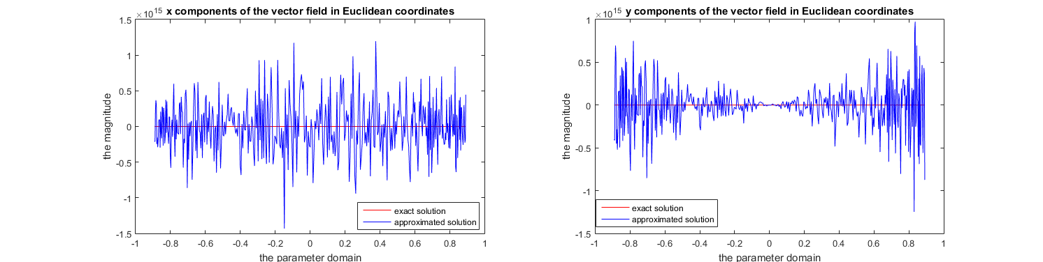
In our numerical test example we assume that $S_{1}^{+}$ is the upper half part of a circle of radius $1$ and $S_{2}$ is an ellipse with short radius $2$ and long radius $3$ . Let $S_{1}^{+}$ be parametrized as the function graph $[x_{1},x_{2}]^{T}=[t,\sqrt{1-t^{2}}]^{T}$ , where $t\in[-0.9,0.9]$ . We use the uniform cubic B-splines to approximate $S_{1}^{+}$ and note it as $S_{1}^{+}[h_{1}]$ . $S_{2}$ is approximated piecewise linearly by polygons $S_{2}[h_{2}]$ . We first test an example of direct reconstruction without regularization, and the results (in Figure 2) shows that the problem is highly ill-posed and the solution by a least square inversion completely losses the expected information.

Taking into account the discretization of the surfaces, we have the functional (4.3) in an approximated form

\left\|F_{h}\mathbf{u}_{h}-\mathbf{y}^{\delta}\right\|^{2}_{L^{2}(S_{2}[h_{2}])}+\left\|n_{h}^{T}\mathbf{u}_{h}\right\|^{2}_{L^{2}(S_{1}[h_{1}])}+\alpha\left|\mathbf{u}_{h}\right|^{2}_{\mathcal{H}^{1}(S_{1}[h_{1}])}.

The corresponding optimality condition is

F_{h}^{\star}F_{h}\mathbf{u}_{h}+n_{h}n_{h}^{T}\mathbf{u}_{h}+\alpha\left(\tau_{h}\partial_{s_{h}}^{2}\langle\mathbf{u},\tau_{h}\rangle+n_{h}\partial_{s_{h}}^{2}\langle\mathbf{u},n_{h}\rangle\right)=F_{h}^{\star}\mathbf{y}^{\delta},

(4.4)

where $\tau_{h}$ and $n_{h}$ denotes the unit tangent and the unit normal vector field on $S_{1}^{+}[h_{1}]$ respectively, and $F_{h}^{\star}$ is the dual operator of $F_{h}$ in $L^{2}$ sense, that is

F_{h}^{\star}\mathbf{y}=\int_{S_{2}[h_{2}]}\mathbf{y}(y)\frac{y-x}{\left|y-x\right|^{2}}ds_{h}(y).

In the implementation, we use linear finite element methods for solving the problem (4.4). In the first example, we reconstruct the magnetization from the noisy data produced from a tangent vector field $\mathbf{u}^{\dagger}=[40x_{1}^{3}x_{2},-40x_{1}^{4}]^{T}$ with $[x_{1},x_{2}]^{T}\in S_{1}^{+}$ the coordinates in ambient space. The results are presented in Figure 3, where we show a selection of plots by varying the noise level $\delta$ and the parameter $\alpha$ , as well as the discretization scale $h$ . The parameters are chosen to satisfy $\delta_{k}=C_{1}\alpha_{k}=C_{2}h_{k}$ with $C_{1}$ and $C_{2}$ are constants, such that the assumption (2.13) is fulfilled. The numerical results in Figure 3 are in accordance with the first statement of Theorem 2.6.

Another set of tests is made to distinguish the behaviour of the two semi-norms which are defined in (3.2) for regularization. In this example, we set the ideal solution to be $\mathbf{u}^{\dagger}(x)=[10x_{2}+5x_{1},5x_{2}-10x_{1}]^{T}$ with $[x_{1},x_{2}]^{T}\in S_{1}^{+}$ , that is a vector field composed with constant amplitudes on both tangent and normal fields of $S_{1}^{+}$ , and we let the noise signal ratio be $NSR=0.5$ in the data. Note that in this example, we do not enforce the tangential constraint, that is we are approximating the minimizer of

\left\|F\mathbf{u}-\mathbf{y}^{\delta}\right\|^{2}_{L^{2}(S_{2})}+\alpha\left|\mathbf{u}\right|^{2}_{{\mathcal{H}}^{1}(S_{1})}.

The numerical results are shown in Figure 4, where the results regularized by using the square of ${H}^{1}(S_{1})$ semi-norm (4.5) are also provided for comparison

\mathcal{R}(\mathbf{u})=\left|\mathbf{u}\right|^{2}_{{H}^{1}(S_{1})}.

(4.5)

We visualize for the regularization parameter which gives the best approximation of the solution. We find that in this particular example, it is not possible to find a good reconstruction by minimizing with the functional (4.5).

4.2 Convergence rates for vector field denoising

We consider denoising of a $2d$ -vector-field $\mathbf{y}^{\delta}=\mathbf{u}^{\delta}$ defined on a $1$ -dimensional curve $S$ . In this example, we have the coincidence of the two surfaces, that is ${\mathcal{M}}_{1}={\mathcal{M}}_{2}=S$ , and $F:{\mathcal{H}}^{1}(S)\rightarrow L^{2}(S)$ is the embedding operator.

Assuming a sequence of approximating curves $(S_{h})_{h\geq 0}$ of $S$ and data $(\mathbf{y}_{h}^{\delta})_{h\geq 0}$ defined on $S_{h}$ , respectively, Tikhonov regularization consists in minimizing the functional

\min_{\mathbf{u}_{h}\in\mathcal{H}^{1}(S_{h})}\left\|\mathbf{u}_{h}-\mathbf{u}^{\delta}\right\|^{2}_{L^{2}(S_{h})}+\alpha\left|\mathbf{u}_{h}\right|^{2}_{\mathcal{H}^{1}(S_{h})}.

In our tests $S$ is the graph of a $sine$ function $[x_{1},x_{2}]^{T}=[t,sin(t)]^{T}$ with $t\in[0,2\pi)$ (cf. Figure 5). $S_{h}$ is approximated by uniform cubic B-splines. In this way, $S_{h}$ is a $C^{2}$ approximation which satisfies Corollary 3.9.

We test for the synthetic solution

	$\displaystyle\mathbf{u}^{\dagger}(x)=$	$\displaystyle 8(x_{2})\tau+4\cos(x_{1})n$
	$\displaystyle=$	$\displaystyle 4\left[\begin{array}[]{c}\frac{2x_{2}\cos(x_{1})-\cos(x_{1})}{\sqrt{1+\cos^{2}(x_{1})}}\\ \frac{2x_{2}+\cos^{2}(x_{1})}{\sqrt{1+\cos^{2}(x_{1})}}\end{array}\right]\text{ for }x=[x_{1},x_{2}]^{T}\in S.$

In this particular example the source condition (2.3) reads as follows:

\left(\tau\partial_{s}^{2}(8x_{2}))+n\partial_{s}^{2}(4\cos(x_{1}))\right)\in L^{2}(S),

which is easy to verify.

For the implementation, we approximate $\mathbf{u}$ by piecewise linear functions with a uniform step size $h_{\mathbf{u}}$ . We denote the discretization size of $S_{h}$ by $h_{s}$ . Then $S_{h}$ contributes a surface disturbance to $S$ with an error bound of the order of $\gamma(h_{s})$ according to our assumption. The results are shown in Table 1, where we selectively show the residuals computed in the experiments. We halve all the parameters for the selected steps, including the regularization parameter $\alpha_{k}$ , the noise level $\delta_{k}$ and the discretization sizes $h_{s,k}$ and $h_{\mathbf{u},k}$ . The parameters then satisfy $\frac{\delta_{k}^{2}}{\alpha_{k}}=\mathcal{O}(\delta_{k})$ , and the order of $\mathcal{O}(\gamma_{k})$ is very close to the order of $\mathcal{O}(\alpha_{k})$ in the tests, that is $\frac{\gamma_{k}^{2}}{\alpha_{k}}=\mathcal{O}(\gamma_{k})$ , $\gamma_{k}=\mathcal{O}(\delta_{k})$ . We find that the numerical rates coincide with the results obtained in the second statement of Theorem 2.6

\left|\check{\mathbf{u}}_{k}-\mathbf{u}^{\dagger}\right|^{2}=\mathcal{O}(\delta_{k}).

Table 1: Convergence rates of vector field denoising on curves

NSR( $\frac{\left\\|\delta\right\\|_{L^{2}}}{\left\\|\mathbf{u}^{\dagger}\right\\|_{L^{2}}}$ )	$1$	$0.5$	$0.25$	$0.125$	$0.625$
$\alpha$	$0.04$	$0.02$	$0.01$	$0.005$	$0.0025$
	$h_{s,1}=0.5\pi$	$\gamma_{1}=1.8371$	$h_{\mathbf{u},1}=0.02\pi$
$\left\|\check{\mathbf{u}}_{1}-\mathbf{u}^{\dagger}\right\|^{2}$	$\mathbf{366.3082}$	$228.1245$	$133.0704$	$77.8783$	$48.6980$
	$h_{s,2}=0.25\pi$	$\gamma_{2}=0.8211$	$h_{\mathbf{u},2}=0.01\pi$
$\left\|\check{\mathbf{u}}_{2}-\mathbf{u}^{\dagger}\right\|^{2}$	$347.8737$	$\mathbf{200.5511}$	$110.7511$	$62.4273$	$37.5464$
	$h_{s,3}=0.125\pi$	$\gamma_{3}=0.3866$	$h_{\mathbf{u},3}=0.005\pi$
$\left\|\check{\mathbf{u}}_{3}-\mathbf{u}^{\dagger}\right\|^{2}$	$276.7971$	$166.7043$	$\mathbf{94.3003}$	$54.0387$	$33.1077$
	$h_{s,4}=0.0625\pi$	$\gamma_{4}=0.1922$	$h_{\mathbf{u},4}=0.0025\pi$
$\left\|\check{\mathbf{u}}_{4}-\mathbf{u}^{\dagger}\right\|^{2}$	$242.3850$	$150.7489$	$90.4440$	$\mathbf{55.0508}$	$34.8112$
	$h_{s,5}=0.03125\pi$	$\gamma_{5}=0.0971$	$h_{\mathbf{u},5}=0.00125\pi$
$\left\|\check{\mathbf{u}}_{5}-\mathbf{u}^{\dagger}\right\|^{2}$	$268.2314$	$158.8666$	$90.0663$	$52.4830$	$\mathbf{32.7122}$

5 Conclusion

In this paper we have studied Tikhonov regularization for solving ill–posed operator equations where the solutions are functions defined on surfaces, and especially we emphasize on the functions with range in vector bundles. Such problems appear in a variety of applications such as recovering magnetization from magnetic potential, vector fields denoising on surfaces and so on. We extended the existing theory on approximation of infinite dimensional Tikhonov regularized solutions for ill–posed operator equations to the surface setting. The theory has been generalized to the case of vector fields, where they are represented by vector valued functions associated to the coordinates in ambient spaces of the surfaces. The additional features of this theory are that it allows to take into account perturbations of the surface and the vector bundle, and it provides an analysis on the convergence and convergence rates which may give an optimal regularization parameter choice.

Acknowledgement

This work has been supported by the Austrian Science Fund (FWF) within the national research network Geometry and Simulation, projects S11704, S11707. Guozhi Dong thanks Christian Gerhards for leading him to the application on magnetization problems and the productive discussions. All the authors thank the reviewers and the editor for their comments to help improving the paper.

Appendix A Background on surfaces and vector fields

Throughout this paper we use some geometrical notations which are collected in Table 2.

Table 2: Notation corresponding to the geometry

Notation	Remark	Notation	Remark
${\mathcal{M}}$	a parametrizable surface	$g$	metric tensor
$m$	mapping $m:\Omega\rightarrow{\mathcal{M}}$	$\partial m$	Jacobian of $m$
$\mathcal{TM}$	tangent vector bundle	$\mathcal{NM}$	normal vector bundle
$\mathcal{P}_{\tau}$	tangent projection	$\mathcal{P}_{n}$	normal projection
$n$	unit normal vector	$g(\cdot,\cdot)$	inner product on $\mathcal{TM}$
$\partial_{i}m$	tangent basis vector

Let $({\mathcal{M}},g)$ be a $d$ -dimensional smooth, oriented, connected and compact surface in $\mathbb{R}^{d+1}$ , which has bounded curvature, and is associated with the Riemannian metric $g$ . To simplify the representation we assume that the surface ${\mathcal{M}}$ is parametrizable, that is ${\mathcal{M}}\subseteq\mathbb{R}^{d+1}$ can be represented by a map $m:\Omega\to\mathbb{R}^{d+1}$ ,

{\mathcal{M}}=m(\Omega),

where $\Omega\subset\mathbb{R}^{d}$ and $m:\Omega\rightarrow{\mathcal{M}}$ is a regular parametrization. In particular we assume that $m$ is bijective and the inverse $m^{-1}:{\mathcal{M}}\rightarrow\Omega$ is also a regular map. $\mathcal{T}_{x}{\mathcal{M}}$ , $\mathcal{N}_{x}{\mathcal{M}}$ denote the tangent and normal vector spaces at $x\in{\mathcal{M}}$ , respectively. Then the tangent and normal bundle are defined by

\mathcal{TM}=\bigcup_{x\in{\mathcal{M}},\;}\left\{(x,\mathbf{v}):\mathbf{v}\in\mathcal{T}_{x}{\mathcal{M}}\right\}

and

\mathcal{NM}=\bigcup_{x\in{\mathcal{M}},\;}\left\{(x,\mathbf{v}):\mathbf{v}\in\mathcal{N}_{x}{\mathcal{M}}\right\}\,,

respectively. We denote by

\partial m(\zeta)=[\partial_{1}m,\partial_{2}m,\cdots,\partial_{d}m](\zeta)\in\mathbb{R}^{(d+1)\times d}

the Jacobian of the parametrization at $x=m(\zeta)\in{\mathcal{M}}$ . The parameters in $\Omega$ are denoted by $\zeta$ . The derivatives with respect to these parameters are always denoted by $\partial$ . The metric tensor $g$ is related to the parametrization $m$ by

g(\zeta)=(\partial m(\zeta))^{T}\partial m(\zeta)\in\mathbb{R}^{d\times d}

(A.1)

on ${\mathcal{M}}$ at $x=m(\zeta)$ . We call a vector field a tangent vector field if $\tilde{\mathbf{v}}:{\mathcal{M}}\rightarrow\mathbb{R}^{d+1}$ with range in the tangent bundle $\mathcal{TM}$ , that is, $\tilde{\mathbf{v}}(x)\in\mathcal{T}_{x}{\mathcal{M}}$ for all $x\in{\mathcal{M}}$ . Every tangent vector $\tilde{\mathbf{v}}(x)\in\mathcal{T}_{x}{\mathcal{M}}$ can be represented in terms of the tangential basis $(\partial_{i}m(\zeta))_{i=1,2,\cdots,d}$ , at each $x=m(\zeta)$ , via

\tilde{\mathbf{v}}(x)=\partial m(\zeta)(\hat{v}_{1}(\zeta),\cdots,\hat{v}_{d}(\zeta))^{T}\in\mathbb{R}^{(d+1)\times 1}.

(A.2)

For two tangent vector field $\tilde{\mathbf{v}}(x)$ and $\tilde{\mathbf{u}}(x)$ , using (A.2), we have the relation

	$\displaystyle g(\tilde{\mathbf{v}},\tilde{\mathbf{u}})$	$\displaystyle:=$	$\displaystyle(\hat{v}_{1}(\zeta),\cdots,\hat{v}_{d}(\zeta))\underbrace{\left(\partial m(\zeta)\right)^{T}\partial m(\zeta)}_{=g(\zeta)}(\hat{u}_{1}(\zeta),\cdots,\hat{u}_{d}(\zeta))^{T}$
		$\displaystyle=$	$\displaystyle\tilde{\mathbf{v}}^{T}\tilde{\mathbf{u}}.$

We denote by $n(x)=(n_{1}(x),n_{2}(x),\cdots,n_{d+1}(x))^{T}\in\mathbb{R}^{d+1}$ the unit normal vector of ${\mathcal{M}}$ at $x\in{\mathcal{M}}$ with fixed orientation, and by $\mathcal{P}_{\tau}$ and $\mathcal{P}_{n}$ the projections onto $\mathcal{T}{\mathcal{M}}$ , $\mathcal{N}{\mathcal{M}}$ at a point $x\in{\mathcal{M}}$ , respectively. They are represented by matrices

\mathcal{P}_{n}(x)=n(x)n(x)^{T}\in\mathbb{R}^{(d+1)\times(d+1)}\quad\text{and}\quad\mathcal{P}_{\tau}(x)=\mathcal{I}-\mathcal{P}_{n}(x)\in\mathbb{R}^{(d+1)\times(d+1)},

(A.3)

where $\mathcal{I}$ is the $(d+1)\times(d+1)$ identity matrix. Because $\mathcal{P}_{\tau}$ and $\mathcal{P}_{n}$ are orthogonal projections on the surface they are satisfying the pointwise estimate

\max\left\{\left|\mathcal{P}_{\tau}\mathbf{u}\right|,\left|\mathcal{P}_{n}\mathbf{u}\right|\right\}\leq\left|\mathbf{u}\right|\;.

In Figure 6 we give a schematic representation of the surface ${\mathcal{M}}$ , its parametrization $m$ over the coordinate domain $\Omega$ , as well as the vector spaces $\mathcal{T}_{x}{\mathcal{M}}$ and $\mathcal{N}_{x}{\mathcal{M}}$ .

Figure 6: Geometry mapping and vector spaces

Lemma A.1.

Let $A\in\mathbb{R}^{(d+1)\times(d+1)}$ , then for every $x\in{\mathcal{M}}$

\left|\mathcal{P}_{\tau}(x)A\right|\leq\left|A\right|\,,\text{ and }\left|\mathcal{P}_{n}(x)A\right|\leq\left|A\right|

(A.4)

where $\left|A\right|$ denotes the Frobenius norm.

Proof.

For every matrix $A$ , $\left|A\right|^{2}=\text{Tr}(A^{T}A)$ , and because $\mathcal{P}_{\tau}(x)$ and $\mathcal{P}_{n}(x)$ are orthogonal projections, we have

	$\displaystyle\left\|A\right\|^{2}$	$\displaystyle=\left\|\mathcal{P}_{\tau}(x)A+\mathcal{P}_{n}(x)A\right\|^{2}$
		$\displaystyle=\text{Tr}\left((\mathcal{P}_{\tau}(x)A+\mathcal{P}_{n}(x)A)^{T}(\mathcal{P}_{\tau}(x)A+\mathcal{P}_{n}(x)A)\right)$
		$\displaystyle=\text{Tr}\left((\mathcal{P}_{\tau}(x)A)^{T}\mathcal{P}_{\tau}(x)A+(\mathcal{P}_{n}(x)A)^{T}(\mathcal{P}_{n}(x)A)\right)$
		$\displaystyle=\text{Tr}\left((\mathcal{P}_{\tau}(x)A)^{T}\mathcal{P}_{\tau}(x)A\right)+\text{Tr}\left((\mathcal{P}_{n}(x)A)^{T}(\mathcal{P}_{n}(x)A)\right)$
		$\displaystyle=\left\|\mathcal{P}_{\tau}(x)A\right\|^{2}+\left\|\mathcal{P}_{n}(x)A\right\|^{2}.$

∎

Moreover, we have the relation between the parametrization and the projection

\mathcal{P}_{\tau}(x)=\partial m(\zeta)g^{-1}(\zeta)(\partial m(\zeta))^{T}

for $x=m(\zeta)$ . We denote by

(\partial m(\zeta))^{\dagger}=g^{-1}(\zeta)(\partial m)^{T}(\zeta)\in\mathbb{R}^{d\times(d+1)},

(A.5)

the Moore-Penrose inverse of the matrix $\partial m(\zeta)\in\mathbb{R}^{(d+1)\times d}$ , which satisfies

(\partial m(\zeta))^{\dagger}\partial m(\zeta)=\operatorname{id}(\zeta)\in\mathbb{R}^{d\times d}\text{ and }\partial m(\zeta)(\partial m(\zeta))^{\dagger}=\mathcal{P}_{\tau}(m(\zeta))\in\mathbb{R}^{(d+1)\times(d+1)}.

Definition A.2.

For a scalar field $v:{\mathcal{M}}\to\mathbb{R}$ , we define its surface gradient at a point $x=m(\zeta)$ by

{\nabla}_{\mathcal{M}}v(x):=\left(\partial(v\circ m)\;(\partial m)^{\dagger}\right)\circ m^{-1}(x)\in\mathbb{R}^{1\times(d+1)}.

(A.6)

The surface gradient fulfills the relation

{\nabla}_{\mathcal{M}}v(m(\zeta))\;\partial m(\zeta)=\partial(v\circ m)(\zeta)\in\mathbb{R}^{1\times d}.

(A.7)

Given a vector valued function $\mathbf{v}:{\mathcal{M}}\rightarrow\mathbb{R}^{d+1}$ , the definition of the gradient with respect to the surface ${\nabla}_{\mathcal{M}}$ consists in taking the gradient of each scalar component $v_{i}$ , i.e., for $x=m(\zeta)$ we have

{\nabla}_{\mathcal{M}}\mathbf{v}(x):=\left(\begin{array}[]{c}{\nabla}_{\mathcal{M}}v_{1}(x)\\ \cdots\\ {\nabla}_{\mathcal{M}}v_{d+1}(x)\end{array}\right)=\left(\partial(\mathbf{v}\circ m)(\zeta)(\partial m(\zeta))^{\dagger}\right)\circ m^{-1}(x)\in\mathbb{R}^{(d+1)\times(d+1)}.

(A.8)

Every vector field $\mathbf{v}:{\mathcal{M}}\rightarrow\mathbb{R}^{d+1}$ can be decomposed into the two vector fields $\mathcal{P}_{\tau}\mathbf{v}$ and $\mathcal{P}_{n}\mathbf{v}$ which have ranges in $\mathcal{T}_{x}{\mathcal{M}}$ and $\mathcal{N}_{x}{\mathcal{M}}$ respectively for all $x\in{\mathcal{M}}$ .

In the following we recall the definition of the covariant derivative of a tangent vector field $\tilde{\mathbf{v}}:{\mathcal{M}}\to\mathcal{TM}$ (see [13, 7]). Equation (A.2) states that

\tilde{\mathbf{v}}(m(\zeta))=\partial m(\zeta)(\hat{v}_{1}(\zeta),\cdots,\hat{v}_{d}(\zeta))^{T}=\sum_{k=1}^{d}\hat{v}_{k}(\zeta)\partial_{k}m(\zeta),

where $\hat{v}_{k}:\Omega\to\mathbb{R}$ denotes the local coordinate representation with respect to the basis $(\partial_{k}m)_{k=1,2,\cdots,d}$ .

Definition A.3 (refering to [7, 6]).

The covariant derivative in direction $k$ with respect to tangent basis $\partial m$ , $(\widetilde{\nabla}_{k}\tilde{\mathbf{v}})_{k=1,2,\cdots,d}$ , is defined by the orthogonal projection of

\partial_{k}(\tilde{\mathbf{v}}\circ m)(\zeta)=\sum_{i=1}^{d}\partial_{k}\hat{v}_{i}(\zeta)\partial_{i}m(\zeta)+\sum_{i=1}^{d}\hat{v}_{i}(\zeta)\partial_{ik}m(\zeta)

into the tangent space. That is, for $x=m(\zeta)$ , the covariant derivative is given by

\widetilde{\nabla}\tilde{\mathbf{v}}(m(\zeta))=\mathcal{P}_{\tau}(m(\zeta))[\partial_{1}(\tilde{\mathbf{v}}\circ m)(\zeta),\cdots,\partial_{d}(\tilde{\mathbf{v}}\circ m)(\zeta)].

(A.9)

In particular for a tangent vector field $\tilde{\mathbf{v}}$ at $x=m(\zeta)$ it follows from (A.9) and (A.8) that

\widetilde{\nabla}\tilde{\mathbf{v}}(x)(\partial m(\zeta))^{\dagger}=\mathcal{P}_{\tau}(x){\nabla}_{\mathcal{M}}\tilde{\mathbf{v}}(m(\zeta)).

(A.10)

Moreover, for an arbitrary vector field $\mathbf{v}:{\mathcal{M}}\to\mathbb{R}^{d+1}$ we have

\widetilde{\nabla}(\mathcal{P}_{\tau}\mathbf{v})(x)(\partial m(\zeta))^{\dagger}=\mathcal{P}_{\tau}(x){\nabla}_{\mathcal{M}}(\mathcal{P}_{\tau}\mathbf{v})(x).

To conclude the appendix, we present a few auxiliary results, which are used to characterize spaces in Section 3.

Lemma A.4.

The gradient operator ${\nabla}_{\mathcal{M}}$ is independent of the parameterization, and fulfils standard rules of differentiation, such as the product rule

1.

Let $v,w:{\mathcal{M}}\to\mathbb{R}$ be differentiable, then

${\nabla}_{\mathcal{M}}(vw)=v{\nabla}_{\mathcal{M}}w+w{\nabla}_{\mathcal{M}}v.$

Moreover, let $\mathbf{v},\mathbf{w},\mathbf{z}:{\mathcal{M}}\to\mathbb{R}^{d+1}$ , then

	$\displaystyle{\nabla}_{\mathcal{M}}(\mathbf{v}^{T}\mathbf{w})$	$\displaystyle=\mathbf{v}^{T}{\nabla}_{\mathcal{M}}\mathbf{w}+\mathbf{w}^{T}{\nabla}_{\mathcal{M}}\mathbf{v},$
	$\displaystyle{\nabla}_{\mathcal{M}}(v\mathbf{w})$	$\displaystyle=\mathbf{w}{\nabla}_{\mathcal{M}}v+v{\nabla}_{\mathcal{M}}\mathbf{w},$
	$\displaystyle{\nabla}_{\mathcal{M}}((\mathbf{v}^{T}\mathbf{w})\mathbf{z})$	$\displaystyle=\mathbf{z}\mathbf{v}^{T}{\nabla}_{\mathcal{M}}\mathbf{w}+\mathbf{z}\mathbf{w}^{T}{\nabla}_{\mathcal{M}}\mathbf{v}+(\mathbf{v}^{T}\mathbf{w}){\nabla}_{\mathcal{M}}\mathbf{z}.$

Lemma A.5.

Let $n(x)=(n_{1}(x),\cdots,n_{d+1}(x))^{T}$ the unit normal vector field on ${\mathcal{M}}$ , and let $\mathbf{v}:{\mathcal{M}}\rightarrow\mathbb{R}^{d+1}$ be a differentiable vector field, then

The following formulas hold

n^{T}{\nabla}_{\mathcal{M}}n=0,\quad\mathcal{P}_{\tau}{\nabla}_{\mathcal{M}}n={\nabla}_{\mathcal{M}}n\text{ and }\mathcal{P}_{\tau}n=0\;,

and

	$\displaystyle\mathcal{P}_{\tau}{\nabla}_{\mathcal{M}}(\mathcal{P}_{\tau}\mathbf{v})$	$\displaystyle=\mathcal{P}_{\tau}{\nabla}_{\mathcal{M}}\mathbf{v}-(n^{T}\mathbf{v}){\nabla}_{\mathcal{M}}n,$
	$\displaystyle\mathcal{P}_{n}{\nabla}_{\mathcal{M}}(\mathcal{P}_{n}\mathbf{v})$	$\displaystyle=\mathcal{P}_{n}{\nabla}_{\mathcal{M}}\mathbf{v}+n\mathbf{v}^{T}{\nabla}_{\mathcal{M}}n.$

Moreover, the seminorm can be represented by

\left|\mathbf{v}\right|^{2}_{{\mathcal{H}}^{1}({\mathcal{M}})}=\left\|{\nabla}_{\mathcal{M}}\mathbf{v}-(n^{T}\mathbf{v}){\nabla}_{\mathcal{M}}n+n\mathbf{v}^{T}{\nabla}_{\mathcal{M}}n\right\|^{2}_{L^{2}(\mathcal{M})}.

Proof.

For the first item, since $n$ is a unit normal vector field,

n^{T}(x)n(x)=1,\quad\forall x\in{\mathcal{M}}.

Then from Lemma A.4 it follows that

2n^{T}(x){\nabla}_{\mathcal{M}}n(x)={\nabla}_{\mathcal{M}}(n^{T}(x)n(x))=0.

Moreover, $\mathcal{P}_{\tau}(x)=\mathcal{I}-n(x)n^{T}(x),$ and thus from the previous it follows that

\mathcal{P}_{\tau}(x){\nabla}_{\mathcal{M}}n(x)=\mathcal{I}{\nabla}_{\mathcal{M}}n(x)-n(x)n^{T}(x){\nabla}_{\mathcal{M}}n(x)={\nabla}_{\mathcal{M}}n(x).

We apply the product rules in Lemma A.4 and properties of $n$ derived above, which show that

	$\displaystyle\mathcal{P}_{\tau}{\nabla}_{\mathcal{M}}(\mathcal{P}_{\tau}\mathbf{v})$	$\displaystyle=\mathcal{P}_{\tau}{\nabla}_{\mathcal{M}}(\mathbf{v}-(n^{T}\mathbf{v})n)$
		$\displaystyle=\mathcal{P}_{\tau}({\nabla}_{\mathcal{M}}\mathbf{v}-nn^{T}{\nabla}_{\mathcal{M}}\mathbf{v}-n\mathbf{v}^{T}{\nabla}_{\mathcal{M}}n-(n^{T}\mathbf{v}){\nabla}_{\mathcal{M}}n)$
		$\displaystyle=\mathcal{P}_{\tau}{\nabla}_{\mathcal{M}}\mathbf{v}-(n^{T}\mathbf{v}){\nabla}_{\mathcal{M}}n,$

and

	$\displaystyle\mathcal{P}_{n}{\nabla}_{\mathcal{M}}(\mathcal{P}_{n}\mathbf{v})$	$\displaystyle=\mathcal{P}_{n}{\nabla}_{\mathcal{M}}((n^{T}\mathbf{v})n)$
		$\displaystyle=\mathcal{P}_{n}(nn^{T}{\nabla}_{\mathcal{M}}\mathbf{v}+n\mathbf{v}^{T}{\nabla}_{\mathcal{M}}n+(n^{T}\mathbf{v}){\nabla}_{\mathcal{M}}n)$
		$\displaystyle=\mathcal{P}_{n}{\nabla}_{\mathcal{M}}\mathbf{v}+n\mathbf{v}^{T}{\nabla}_{\mathcal{M}}n.$

Adding the two identities, and using the orthogonality of $\mathcal{P}_{\tau}$ and $\mathcal{P}_{n}$ on $L^{2}(\mathcal{M})$ , we get the second item from Definition 3.2:

		$\displaystyle\left\\|{\nabla}_{\mathcal{M}}\mathbf{v}-(n^{T}\mathbf{v}){\nabla}_{\mathcal{M}}n+n\mathbf{v}^{T}{\nabla}_{\mathcal{M}}n\right\\|^{2}_{L^{2}(\mathcal{M})}$
	$\displaystyle=$	$\displaystyle\left\\|\mathcal{P}_{\tau}{\nabla}_{\mathcal{M}}(\mathcal{P}_{\tau}\mathbf{v})+\mathcal{P}_{n}{\nabla}_{\mathcal{M}}(\mathcal{P}_{n}\mathbf{v})\right\\|^{2}_{L^{2}(\mathcal{M})}$
	$\displaystyle=$	$\displaystyle\left\\|\mathcal{P}_{\tau}{\nabla}_{\mathcal{M}}(\mathcal{P}_{\tau}\mathbf{v})\right\\|^{2}_{L^{2}(\mathcal{M})}+\left\\|\mathcal{P}_{n}{\nabla}_{\mathcal{M}}(\mathcal{P}_{n}\mathbf{v})\right\\|^{2}_{L^{2}(\mathcal{M})}$
	$\displaystyle=$	$\displaystyle\left\|\mathbf{v}\right\|^{2}_{{\mathcal{H}}^{1}({\mathcal{M}})}.$

This concludes the proof. ∎

References

[1] J.H. Ahlberg, E.N. Nilson. Convergence properties of the spline fit. J. Soc. Indust. Appl. Math., 11(1):95–104, 1963.
[2] A. N. Tikhonov and V. Y. Arsenin. Solutions of Ill-Posed Problems. John Wiley & Sons, Washington, D.C., 1977.
[3] C. W. Groetsch. The Theory of Tikhonov Regularization for Fredholm Equations of the First Kind. Pitman, Boston, 1984.
[4] V. A. Morozov. Methods for Solving Incorrectly Posed Problems. Springer, New York, Berlin, Heidelberg, 1984.
[5] A. Neubauer and O. Scherzer. Finite-dimensional approximation of Tikhonov regularized solutions of nonlinear ill-posed problems. Numer. Funct. Anal. Optim., 11(1-2):85–99, 1990.
[6] B. A. Dubrovin, A.T. Fomenko, and S.P. Novikov. Modern Geometry - Methods and Applications: Part I: The Geometry of Surfaces, Transformation Groups, and Fields. Graduate Texts in Mathematics. Spinger, 2 edition, 1991. Tanslated by Burns, R.G.
[7] M. P. do Carmo. Riemannian Geometry. Birkhäuser, 1992.
[8] A.B. Bakushinskii and A.V. Goncharskii. Ill-Posed Problems: Theory and Applications. Kluwer Academic Publishers, Dordrecht, Boston, London, 1994.
[9] A. N. Tikhonov, A. Goncharsky, V. Stepanov, and A. Yagola. Numerical Methods for the Solution of Ill-Posed Problems. Kluwer, Dordrecht, 1995.
[10] R. Blakely. Potential Theory in Gravity and Magnetic Applications. Cambridge University Press, Cambridge, 1996.
[11] H. W. Engl, M. Hanke, and A. Neubauer. Regularization of inverse problems, volume 375 of Mathematics and its Applications. Kluwer Academic Publishers Group, Dordrecht, 1996.
[12] G. H. Golub, and Ch. F. Van Loan, Matrix Computations. The Johns Hopkins University Press, Baltimore, 1996.
[13] J. M. Lee. Riemannian surfaces, volume 176 of Graduate Texts in Mathematics. Springer-Verlag, New York, 1997. An introduction to curvature.
[14] V. P. Tanana. Methods for solution of nonlinear operator equations. Inverse and Ill-posed Problems Series. VSP, Utrecht, 1997.
[15] A. N. Tikhonov, A. S. Leonov, and A. G. Yagola. Nonlinear ill-posed problems. Vol. 1, 2, volume 14 of Applied Mathematics and Mathematical Computation. Chapman & Hall, London, 1998. Translated from the Russian.
[16] E. Hebey. Nonlinear analysis on manifolds: Sobolev spaces and inequalities, volume 5 of CIMS Lecture Notes. New York University, 1999.
[17] M. Burger and S. Osher. Convergence rates of convex variational regularization. Inverse Probl., 20(5):1411–1421, 2004.
[18] J. Kaipio and E. Somersalo. Statistical and Computational Inverse Problems, volume 160 of Applied Mathematical Sciences. Springer Verlag, New York, 2005.
[19] E. Resmerita and O. Scherzer. Error estimates for non-quadratic regularization and the relation to enhancement. Inverse Probl., 22(3):801–814, 2006.
[20] B. Hofmann, B. Kaltenbacher, C. Pöschl, and O. Scherzer. A convergence rates result for Tikhonov regularization in Banach spaces with non-smooth operators. Inverse Probl., 23(3):987–1010, 2007.
[21] J. Lefèvre and S. Baillet. Optical flow and advection on 2-Riemannian surfaces: A common framework. IEEE Trans. Pattern Anal. Mach. Intell., 30(6):1081–1092, June 2008.
[22] O. Scherzer, M. Grasmair, H. Grossauer, M. Haltmeier, and F. Lenzen. Variational methods in imaging, volume 167 of Applied Mathematical Sciences. Springer, New York, 2009.
[23] P.C. Hansen. Discrete inverse problems, volume 7 of Fundamentals of Algorithms. SIAM, Philadelphia, PA, 2010.
[24] C. Pöschl, E. Resmerita, and O. Scherzer. Discretization of variational regularization in Banach spaces. Inverse Probl., 26(10):105017, 2010.
[25] D. Gubbins, D. Ivers, S. M. Masterton and D. E. Winch. Analysis of lithospheric magnetization in vector spherical harmonics,. Geophys. J. Int., 187(1):99–117, 2011.
[26] J. L. Mueller and S. Siltanen. Linear and nonlinear inverse problems with practical applications, volume 10 of Computational Science & Engineering. Society for Industrial and Applied Mathematics (SIAM), Philadelphia, PA, 2012.
[27] T. Schuster, B. Kaltenbacher, B. Hofmann, and K. S. Kazimierski. Regularization methods in Banach spaces, volume 10 of Radon Series on Computational and Applied Mathematics. Walter de Gruyter GmbH & Co. KG, Berlin, 2012.
[28] C. Kirisits, L. F. Lang, and O. Scherzer. Optical flow on evolving surfaces with an application to the analysis of 4D microscopy data. In A. Kuijper, K. Bredies, T. Pock, and H. Bischof, editors, SSVM’13: Proceedings of the 4th International Conference on Scale Space and Variational Methods in Computer Vision, volume 7893 of Lecture Notes in Computer Science, pages 246–257, Berlin, Heidelberg, 2013. Springer-Verlag.
[29] C. Kirisits, L. F. Lang, and O. Scherzer. Optical flow on evolving surfaces with space and time regularisation. J. Math. Imaging Vision, 52(1):55–70, 2015.
[30] C. Kirisits, C. Pöschl, E. Resmerita, and O. Scherzer. Finite-dimensional approximation of convex regularization via hexagonal pixel grids. Appl. Anal., 94(3):612–636, 2015.
[31] C. Gerhards. On the unique reconstruction of induced spherical magnetizations. Inverse Probl., 32(1):1–24, 2016.

$\displaystyle\left\\|F_{k}\mathbf{u}^{\dagger}_{k}-\mathbf{y}_{k}\right\\|_{2,k}^{2}$	$\displaystyle=\left\\|T_{2,k}T_{2,k}^{-1}(F_{k}\mathbf{u}^{\dagger}_{k}-\mathbf{y}_{k})\right\\|_{2,k}^{2}$	(2.16)
	$\displaystyle\leq C\left\\|T_{2,k}^{-1}(F_{k}\mathbf{u}^{\dagger}_{k}-\mathbf{y}_{k})\right\\|_{2}^{2}$
	$\displaystyle=C\left\\|T_{2,k}^{-1}F_{k}T_{1,k}\mathbf{u}^{\dagger}-F\mathbf{u}^{\dagger}+\mathbf{y}-T_{2,k}^{-1}\mathbf{y}_{k}\right\\|_{2}^{2}$
	$\displaystyle=\mathcal{O}(\rho_{k}^{2}+\gamma_{2,k}^{2}+\delta_{k}^{2}),$

$\displaystyle\left\\|(n^{T}\mathbf{u}){\nabla}_{\mathcal{M}}n\right\\|_{L^{2}(\mathcal{M})}^{2}$	$\displaystyle=\int_{\mathcal{M}}\left\|(n^{T}\mathbf{u}){\nabla}_{\mathcal{M}}n\right\|^{2}ds(x)$	(3.6)
	$\displaystyle\leq\left\\|\nabla_{\mathcal{M}}n\right\\|^{2}_{L^{\infty}({\mathcal{M}})}\int_{\mathcal{M}}\left\|\left<n,\mathbf{u}\right>\right\|^{2}\,ds(x)$
	$\displaystyle\leq C_{c}^{2}\int_{\mathcal{M}}\left\|\mathbf{u}\right\|^{2}\,ds(x)\;.$

$\displaystyle\left\\|\mathcal{P}_{n}{\nabla}_{\mathcal{M}}\mathcal{P}_{n}\mathbf{u}\right\\|_{L^{2}(\mathcal{M})}$	$\displaystyle=\left\\|\mathcal{P}_{n}{\nabla}_{\mathcal{M}}\mathbf{u}+n\mathbf{u}^{T}{\nabla}_{\mathcal{M}}n\right\\|_{L^{2}(\mathcal{M})}$	(3.8)
	$\displaystyle\leq\left\\|\mathcal{P}_{n}{\nabla}_{\mathcal{M}}\mathbf{u}\right\\|_{L^{2}(\mathcal{M})}+\sqrt{\int_{\mathcal{M}}\left\|n\mathbf{u}^{T}{\nabla}_{\mathcal{M}}n\right\|^{2}\,ds(x)}$
	$\displaystyle\leq\left\\|\mathcal{P}_{n}{\nabla}_{\mathcal{M}}\mathbf{u}\right\\|_{L^{2}(\mathcal{M})}+\sqrt{\int_{\mathcal{M}}\left\|n\mathbf{u}^{T}\right\|^{2}\left\|{\nabla}_{\mathcal{M}}n\right\|^{2}\,ds(x)}$
	$\displaystyle\leq\left\\|\mathcal{P}_{n}{\nabla}_{\mathcal{M}}\mathbf{u}\right\\|_{L^{2}(\mathcal{M})}+C_{c}\sqrt{\int_{\mathcal{M}}\left\|n\mathbf{u}^{T}\right\|^{2}\,ds(x)}\;.$

$\displaystyle\left\\|{\nabla}_{\mathcal{M}}\mathbf{u}\right\\|_{L^{2}(\mathcal{M})}$	$\displaystyle\leq$	$\displaystyle\left\\|{\nabla}_{\mathcal{M}}\mathbf{u}-n^{T}\mathbf{u}{\nabla}_{\mathcal{M}}n+n\mathbf{u}^{T}{\nabla}_{\mathcal{M}}n\right\\|_{L^{2}(\mathcal{M})}$
		$\displaystyle\quad+\left\\|n^{T}\mathbf{u}{\nabla}_{\mathcal{M}}n\right\\|+\left\\|n\mathbf{u}^{T}{\nabla}_{\mathcal{M}}n\right\\|_{L^{2}(\mathcal{M})}$
	$\displaystyle\leq$	$\displaystyle\left\|\mathbf{u}\right\|_{{\mathcal{H}}^{1}({\mathcal{M}})}+2C_{c}\left\\|\mathbf{u}\right\\|_{L^{2}(\mathcal{M})}.$

	$\displaystyle\left\|{\widetilde{\mathbf{u}}}\right\|_{{\widetilde{\mathcal{H}}_{\mathcal{T}}^{1}({\mathcal{M}})}}^{2}$	$\displaystyle=\int_{\mathcal{M}}\left\|\mathcal{P}_{\tau}(x){\nabla}_{\mathcal{M}}{\widetilde{\mathbf{u}}}(x)\right\|^{2}ds(x)$
		$\displaystyle\underbrace{=}_{\eqref{eq:cov_m_t}}\int_{\mathcal{M}}\left\|(\widetilde{\nabla}{\widetilde{\mathbf{u}}}(x)(\partial m(\zeta))^{\dagger})\right\|^{2}ds(x)$
		$\displaystyle=\int_{\mathcal{M}}\text{Tr}\left(\left(\widetilde{\nabla}{\widetilde{\mathbf{u}}}(x)(\partial m(\zeta))^{\dagger})\right)\left(\widetilde{\nabla}{\widetilde{\mathbf{u}}}(x)(\partial m(\zeta))^{\dagger})\right)^{T}\right)ds(x)$
		$\displaystyle\underbrace{=}_{\eqref{eq:projectiona}}\int_{\mathcal{M}}\text{Tr}\left(\left(\widetilde{\nabla}{\widetilde{\mathbf{u}}}(x)\right)g^{-1}\left(\widetilde{\nabla}{\widetilde{\mathbf{u}}}(x)\right)^{T}\right)ds(x),$