Improved Solution to the Non-Domination Level Update Problem
Abstract
Non-domination level update problem is to sort the non-dominated fronts after insertion or deletion of a solution. Generally the solution to this problem requires to perform the complete non-dominated sorting which is too expensive in terms of number of comparisons. Recently an Efficient Non-domination Level Update (ENLU) approach is proposed which does not perform the complete sorting. For this purpose, in this paper a space efficient version of ENLU approach is proposed without compromising the number of comparisons. However this approach does not work satisfactorily in all the cases. So we have also proposed another tree based approach for solving this non-domination level update problem. In case of insertion, the tree based approach always checks for same number of fronts unlike linear approach in which the number of fronts to be checked depends on the inserted solution. The result shows that in case where all the solutions are dominating in nature the maximum number of comparisons using tree based approach is as opposed to in ENLU approach. When all the solutions are equally divided into fronts such that each solution in a front is dominated by all the solutions in the previous front then the maximum number of comparisons to find a deleted solution in case of tree based approach is less than that of ENLU approach. Using these approaches an on-line sorting algorithm is also proposed and the competitive analysis of this algorithm is also presented.
I Introduction
In past few decades the evolutionary algorithms [1], [2], [3], [4] have gained a lot of popularity. One of the primarily reason behind its popularity is their ability to solve real world problems. Real world problems may involve simultaneous optimizing multiple objectives. Thus the evolutionary algorithms also optimize single as well as multiple objectives. In case of single objective optimization, only single solution is optimal one. But in case of multi-objective optimization problems (MOOPs) [5], [6], [7], [8] a set of set of optimal solutions are achieved and these are known as Pareto-optimal solutions.
In literature various multi-objective evolutionary algorithms (MOEAs) are proposed. Some of them are non-dominated sorting genetic algorithm II (NSGA-II) [9], strength pareto evolutionary algorithm 2 (SPEA2) [10], pareto archive evolution strategy (PAES) [11], pareto envelope-based selection algorithm (PESA) [12] and pareto frontier differential evolution (PDE) [13] etc. These MOEAs are able to find a set of Pareto optimal solutions in one single run. There exist various approaches for the selection of solutions [14]. But the Pareto-based approach is generally used. Non-dominated sorting [9] is found to be efficient for finding Pareto-optimal solution out of various techniques.
In this sorting the solutions are assigned to their respective front based on their dominance relationship. This process is time consuming when the number of solutions in the populations becomes larger. Much work [9], [15], [16] has been done to improve the running time of this process. Golberg et al. [17] first proposed the idea of non-dominated sorting. Later this idea was used in multi-objective genetic algorithm [18].
Let be the population of solutions. These solutions are categorized into fronts. These fronts are denoted as . The solutions which belong to front are dominated by at-least one of the solutions belonging to front , . Let the number of solutions in each front is . Thus . The arrangement of the solutions in each front is shown in Table I. Consider an example.
Example I.1
Let be a set of solutions. Two objectives are associated with each solution. Let both the objectives are to be minimized. These solutions are arranged in fronts. The arrangement of solutions in each fronts is as follows: , , , , .
| Front | Solutions |
| ⋮ | ⋮ |
The generational Evolutionary Multi-Objective Optimization (EMO) algorithms generate all the offspring solutions from the parent solutions. Then they both are compared. As opposite to the generational EMO algorithms, steady state EMO algorithms [19], [20] update the parent population as a new offspring is derived. The steady state EMO algorithms have the ability to generate the good offspring solutions. The parallel implementation is also possible with this kind of EMO algorithms.
There have not been so many such kind of EMO algorithms proposed [21]. One of the primarily reason for this is the overhead in repeatedly performing the non-dominated sorting as a new solution is generated or an existing solution is removed. But when either a new solution in inserted or an existing solution is removed then not all the solutions change its domination level so it is un-necessary to perform the complete non-dominated sorting again and again. Only some of the solutions need to change their non-domination level. This is first addressed in [21]. Li at al. [21] proposed an efficient non-domination level update (ENLU) approach for steady-state EMO algorithms. They have proposed the approach for insertion as well as deletion. In this approach not all the solutions change their domination level. The solutions which need to change their domination level, only change the level. After this some more work has been carried out in this direction [22], [23]. But these two work focus on bi-objective steady state EMO algorithms. So in this paper we have proposed the modified version of ENLU which is efficient in terms of space and time complexity remains the same. One more approach is provided which is based on tree data structure. The maximum number of dominance comparison while performing insertion or deletion is also obtained. In short the main contribution are as follows:
- •
The modified linear approach with space requirement as opposite to in [21] is proposed.
- •
The dominance tree based approach is proposed for non-domination level update problem.
- •
We have obtained the maximum number of dominance comparisons occurred in linear as well as dominance tree based approach.
- •
The approach for searching a solution is also proposed using dominance tree.
- •
The solution to the non-domination level update problem can be used as a non-dominated sorting algorithm. This sorting algorithm can be used as on-line algorithm. The competitive ratio of this on-line algorithm is also obtained.
The rest of this paper is organized as follows. Section II describes the Non-domination Level Update problem. The related work is also described in this Section. The modified linear approach to insert a solution in the given set of fronts is discussed in Section III. The Proposed dominance binary search tree based approach is illustrated in Section IV. The look up procedure using dominance binary search tree based approach is provided in Section V. The procedure to delete an existing solution is discussed in Section VI. Section VII discuss the maximum number of dominance comparison in Non-domination Level Update problem. In section VIII and IX we discuss the maximum and minimum number of dominance comparison in two cases when al the solutions are non-dominating and when all are dominating respectively. The sorting algorithm using the proposed approach is presented in Section X. Finally Section XI concludes the paper and provides the future direction of the work.
II Non-domination Level Update problem
In this section we discuss the non-domination level update problem. Non-domination Level Update problem is to sort the non-dominating front after insertion of a new solution or after deletion of an existing solution. Let be the set of solutions. Let objectives are associated with these solutions. These solutions are divided into fronts. Let be the set of fronts in decreasing order of their dominance i.e., the first front is having rank (non-domination level ), second is having rank and so on. The number of solutions in each front is given by , . Thus . Table I shows this scenario.


Let a new solution new is to be inserted into the set of fronts. Non-domination Level Update problem in case of insertion is to insert this new solution at its correct position in the set of fronts and update the fronts if needed. Figure 1(a) clearly shows this situation. In this figure, there are solutions. Let be the set of these solutions. These solutions are divided into fronts. Let be the set of fronts in the decreasing order of their dominance. , , , . A new solution new is to be inserted in the set of fronts. Main aim here is to update after insertion of new. Figure 1(b) shows the updated set of fronts when new solution is inserted in the set of fronts.
Let an existing solution is to be deleted from the set of fronts. Non-domination Level Update problem in case of deletion is to delete this solution and update the set of fronts if required. Figure 1(a) shows the set of fronts. An existing solution is to be deleted from the set of fronts. The motive is to update after deletion of solution . Figure 1(c) shows the updated set of fronts when solution is being deleted from the set of fronts.
The naive approach is to apply the non-dominated sorting algorithm on all the solutions along with new solution in case of insertion or apply the non-dominated sorting algorithm on the remaining solutions in case of deletion. Thus the complete sorting algorithm is to be applied on either or solutions. If we use the brute-force technique then the time complexity will be and space requirement will be . When the fast non-dominating sorting proposed in [9] is used then the time complexity will be . This always requires dominance comparison in case of insertion and comparison in case of deletion regardless of arrangement of fronts. The space requirement will be . Tang et al. [24] proposed arena’s principle. The time complexity of their approach is in worst case. The space requirement is . McClymont et al. [15] proposed two sorting algorithms - climbing sort and deductive sort. The climbing sort requires comparison in case of insertion and comparison in case of deletion when the worst case scenario occurs. The space requirement is . The deductive sort has some advantage over climbing. In the worst case the number of comparison is for insertion and for deletion. The space requirement is as opposite to by climbing sort. The approach proposed in [16] requires time in worst case. In the worst case the total number of dominance comparison is same as deductive sort. This approach first sorts the solutions based on first objective which also requires time. The space requirement of this approach is .
All the above discussed approaches apply the complete sorting algorithm on either or solutions. To reduce the number of dominance comparisons without applying the complete sorting algorithm, Li et al. [21] proposed an approach for Non-domination Level Update problem. The approach was proposed for Steady-State Evolutionary Multiobjective Optimization. The time complexity is in case of equal division of solutions in fronts. However the worst case time complexity is [22], [23]. The space requirement is as the dominated solution is kept at tow places - one is in archive and other is in front .
Yakupov et al. [22] proposed an incremental non-dominated sorting for bi-objective solutions. The running time of the approach is which is in worst case when a new solution is inserted in the set of fronts having solutions with objectives. With further improvement in this work, Buzdalov et al. [23] proposed fast implementation of the steady-State NSGA-II algorithm for two dimensions based on incremental non-dominated sorting. In this work, the support of the crowding distance calculation is employed. After that, the steady-state version of the NSGA-II algorithm is presented. In [22] and [23] a data structure tree of tress is used. The nodes in higher level tree stores the number of tree elements in a sub-tree, the previous-in-order node and the next-in-order node. Thus extra space is required which is . The nodes in lower level tree also stores the number of tree elements in a sub-tree, the previous-in-order node and the next-in-order node. Thus extra space is required which is . Thus the space requirement is .
We have proposed an approach based on dominance binary search tree. First we discuss the modified version of linear approach proposed in [21] for insertion as well as deletion. The modification is done to reduce the space complexity from to .
III Modified Linear Approach: Insert a Solution
In this section we will discuss the Non-domination Level Update problem using linear way to obtain the correct position of new solution new as done in [21]. Algorithm 1 shows the insertion procedure of new in the list of non-dominated fronts . This algorithm does not run the complete sorting algorithm again. It uses the non-dominance properties of the solution in the same front and uses the ranking of the front. Here we are assuming that all the fronts are arranged in decreasing order of their dominance. The process for inserting a solution is summarized in Algorithm 1. Two solutions are compared for dominance nature using domNature(A,B) procedure which returns the following three values.
- •
1: Solution dominates .
- •
-1: Solution is dominated by .
- •
0: Solution and are non-dominated.
The new solution new is compared with all the fronts in sequential manner starting from to . new is compared with each solution in a front. When new is compared with any solution in a front then there are three possibilities:
1. If the solution in the front dominates new it means new can not be inserted into . So now we check for another front having lower dominance without checking it with other solutions in the same front. If then new creates a new front having lowest dominance among all the fronts.
2. If the solution in the front is non-dominating with the new then we keep on comparing new with rest of the solutions in that front. If new is non-dominating with all the solutions in the front then new is added in the front .
3. If new dominates the solution in the front then we obtain the list of all the solutions in the front which are dominated by new using DomSet() procedure as described in Algorithm 2. This DomSet() procedure returns the list of all the solutions in front which are dominated by new. The solutions which are dominated by new are removed from front . After the removal of dominated solution in , new is added to . Now we have the following possibilities:
- •
If then creates a new front having lowest dominance among all the fronts.
- •
If new dominates all the solutions in the front (after removing the dominated solutions from and adding new to the cardinality of is ) i.e. then the dominance level of all the fronts are increased by one and dominated solution is assigned to front .
- •
If none of the above two conditions are satisfied i.e. new dominates some of the solutions in front and then UpdateInsert() procedure is used which re-arranges the solutions in their respective front. This UpdateInsert() procedure is discussed in Algorithm 3.
III-A Illustration of DomSet procedure
This procedure takes as input a front , new solution , the index of the solution in the front from where the dominance of new needs to be checked and set of solutions dominated by new . This procedure returns the updated set of solutions dominated by new in front . For this purpose new is checked against all the solutions in the front starting from index position. The solution which is dominated by new is added to and removed from the front . We are removing the dominated solutions from the front to save the space. In this manner same solution does not occupy more than one place.
Complexity Analysis: In the worst case, all the solutions in the front except first is compared with new solution in the DomSet() procedure so the worst case complexity of DomSet() procedure becomes .
III-B Illustration of UpdateInsert procedure
This procedure takes as input the set of non-dominated fronts , a set of solution , the index of the front denoted by index in . This procedure updates the by either creating a new front or by re-arranging the solutions in the existing fronts. First of all the initial cardinality of is stored is . This is because when the solutions from is compared with for non-dominance then it should be compared with only first solutions.
Here we find the solutions in which are non-dominated with . The solutions which are non-dominated with are added to it and removed from . The removal guarantees that no solution can occupy more than one place. Now the following situation can occur:
- •
If no solution from is being added to i.e. then the dominance level of fronts is increased by and is assigned the dominance level index.
- •
If all the solutions from is added to i.e. then make as .
- •
Otherwise all the solutions from is moved to . The movement means as a solution from is moved to , the solution is being removed from . The non-domination level of is assigned to . The procedure is repeated with UpdateInsert.
Complexity Analysis: In this algorithm the maximum number of comparison is performed when new dominates the solutions in the first front i.e. this procedure is called with . For maximum number of comparison, the . The maximum number of comparison occurs when each call to this procedure shifts one solution in higher level front after comparing with all the solutions. Thus the maximum number of comparison for this procedure is given by . Each comparison between two solutions requires at-most comparison between objectives. Thus the worst case complexity of this procedure is . The best case occurs when has single solution and is non-dominating with this solution. In this case only one comparison is required so the best case complexity is .
III-C Complexity of Modified Linear Approach
Here we will analyze the complexity using the linear approach. We can see from all the algorithms 1, 2 and 3 that no solution is being kept at more than one place. Only few scaler variables are required. Therefore, the space complexity of linear approach is . The worst case time complexity of UpdateInsert() procedure dominates the worst case time complexity of DomSet() procedure. The complexity of UpdateInsert() procedure is quadratic while DomSet() has linear complexity. Thus the overall worst case complexity of the modified approach is . This time complexity is same as proposed in [21].
IV Proposed Approach using Dominance Binary Search Tree
In this section we will discuss the proposed approach for Non-domination Level Update problem using dominance tree. This approach inserts the new solution to its correct position using tree based methodology unlike linear way as proposed in [21]. The only difference between the linear approach and tree based approach is in identifying the position of the inserted solution. The update procedure remains the same. Thus dominance tree based approach will be beneficial when there are large number of fronts. We first provide formal definition of this tree. Two variants of this tree are also discussed.


The tree based data structure is also used in [22] and [23]. The authors have used tree of trees where the high level tree corresponds to the non-dominated front i.e. node in the high level tree corresponds to a front. The low level tree corresponds to the solutions inside a front i.e. the nodes in the low level tree corresponds to solutions inside the front. The solutions in the low level tree are sorted according to first objective. The high-level tree can be an ordinary balanced tree while the low level tree should be a split-merge tree. The uses of this data structure perform some of the operations in time like element search in the container, splitting of container by key into two parts and merging of two container. In [23], Cartesian Tree [25] is used as a split-merge tree as it performs better than the Splay Tree [26] in practice.
We have used only high level tree named as Dominance Binary Search Tree. The solutions inside a node are arranged in linear fashion. Thus no sorting is required.
IV-A Dominance Binary Search Tree
In Dominance Binary Search Tree, the node represents single non-dominated front i.e., the solutions in a node are non-dominating with each other.
Definition 1 (Dominance Binary Search Tree)
A binary tree is known as Dominance Binary Search Tree if the node is having lower dominance than left sub-tree and higher dominance than right sub-tree.
Example IV.1
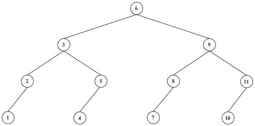
Let be the set of non-dominated fronts in decreasing order of their dominance i.e., the first front is having rank 1 (higher rank), second is having rank and so on. The corresponding Dominance Binary Search Tree is given in Figure 2(a).
Dominance binary search tree can be categorized into two types based on how the root of a sub-tree is chosen.
- 1.
Left-Balanced Dominance Binary Search Tree: If left child of each node is filled before the right child then the tree is called left-balanced dominance binary search tree. It is obtained when the index of the root of a sub-tree is calculated as . See Figure 2(b).
- 2.
Right-Balanced Dominance Binary Search Tree: If right child of each node is filled before the left child then the tree is called right-balanced dominance binary search tree. It is obtained when the index of the root of a sub-tree is calculated as . See Figure 2(c).
Unlike the linear approach where new needs to be compared with all the fronts in the worst case, here the solution is compared with either or fronts in all the cases. The process to insert a new solution new in the set of fronts is summarized in Algorithm 4.
IV-B Illustration of Algorithm 4
Algorithm 4 shows the insertion procedure of a new solution in the fronts using dominance binary search tree approach. Here like linear approach, we are also assuming that all the fronts are arranged in decreasing order of their dominance. This insertion can make the following changes in the tree.
- I.
new can make new front i.e., creation of a new node.
- II.
new can be merged with any of the existing fronts.
- III.
new can be merged with any of the fronts by removing some of the solutions (which are dominated by ) in that front. After this removal, the solutions in the lower dominance fronts are re-arranged.
With the help of Algorithm 4 a new solution new is inserted in the given list of fronts. If there is only single front then Algorithm 1 is called. Here the insertion is performed in the same manner as in linear approach. So in case of single front i.e. when all the solutions are non-dominating in nature then the linear approach and dominance tree based approach is same. If the number of fronts are more than one then the dominance binary search tree approach comes into picture. This algorithm first executes Algorithm 5 which gives a list known as CmpFront. In place of Algorithm 5 which is based on Left Dominance Binary Search Tree, Algorithm 6 can also be used which is based on Right Dominance Binary Search Tree.
Algorithm 5 and 6 returns a list CmpFront. Each element of this list is 3-folded - dom,fIndex,sIndex. ‘dom’ is the dominating nature of new with a particular solution in the front. ‘fIndex’ is the index of the front to which the new is compared and ‘sIndex’ is the index of the solution in to which new is compared and ’dom’ is achieved. Thus ‘dom’ shows the dominated nature of new with . The ‘dom’ can take three values . The value of ‘fIndex’ can vary between to . Generally the value of ‘sIndex’ can vary between to but when new is non-dominating with all the solutions in a particular front then the value of ‘sIndex’ is . The maximum length of this list is because the maximum number of fronts to which new can be compared is .
After obtaining CmpFront, the correct position of new is to be identified. Let the length of CmpFront is denoted by len. There are following possibilities:
If last node in the CmpFront is non-dominating with new then new will be inserted in the front corresponding to last node. The index of the front corresponding to last node is obtained by .
If new dominates last node in the CmpFront then
- I.
Obtain the index of the front corresponding to last node. The index of this node, .
- II.
Obtain the index of the solution which is first dominated by new in the . The index of this solution, .
- III.
Add the solution in
- IV.
Remove the solution from
- V.
Obtain rest of the dominated solution in by new using DomSet() procedure. The DomSet() is called with following parameter - , new, sIndex+1 and .
- VI.
After obtaining , new is being added to . Now one of the following three possibilities may arise:
- •
If then creates a new front having lowest dominance.
- •
If new dominates all the solutions in front i.e. then the dominance level of all the fronts are increased by and is assigned to front .
- •
If none of the above two conditions are satisfied then UpdateInsert() procedure is used which re-arranges the solutions in their respective fronts. The UpdateInsert() is called with following parameter - , and .
- •
If the values denoting dominance nature of new in CmpFront list contains for all the fronts i.e. new is dominated by all the compared fronts. Formally . In this case it is clear that new will make another front which is having lower dominance than all the existing fronts.
The CmpFront list is traversed backward i.e. from the end to start. If the two consecutive values denoting dominance nature of new in CmpFront list are different then the position of new is identified otherwise we move to next CmpFront element. Formally for the position of new is to be identified . If this condition is met and if the dominating value of next front (current front is i and next front is i-1) is then the new will be inserted in the next front. If dominating value of next front is then UpdateInsert() procedure is called with following parameter - , and .
IV-C Illustration of InsertTree_Left() procedure
Initially new is compared with the root of the tree. The index of the root is calculated as .
1. If any solution in the root dominates new then the new will be having lower dominance than the root. So the algorithm explore the right sub-tree of the root using recursive procedure InsertTree_Left().
2. If new and solution in the root is non-dominating then we continue dominance comparison of new with rest of the solutions in the root. If new is non-dominating with rest of the solutions in the root then new can not have lower dominance than root. But it can have higher dominance than the root so for this the left sub-tree is explored using recursive procedure InsertTree_Left().
3. If new dominates the solution in the node then the new has higher dominance than the root node so the left-sub tree of the root is explored using recursive procedure InsertTree_Left().
Terminating Condition of Algorithm 5 and 6: The terminating condition depends on how the index of the root of a sub-tree i.e. mid is calculated. It depends on whether the tree is Left-Balanced or Right-Balanced. The procedure terminates when any one of the following conditions are satisfied.
- 1.
A leaf node is encountered.
- 2.
If the tree is Left-Balanced Dominance Binary Search Tree and a node with single child is encountered which dominates new.
- 3.
If the tree is Right-Balanced Dominance Binary Search Tree and a node with single child is encountered which does not dominate new.
Complexity Analysis: The maximum number of fronts to which new is compared is . Each comparison to the front adds an element in the list CmpFront. Thus the space complexity of the proposed algorithm is . In the worst case, the new is to be checked for dominance with all the solutions in the compared fronts. If there is equal division of solutions in all the fronts i.e. each front has solutions then the complexity of the algorithm 5 and 6 is which is is worst case.
IV-D Complexity Analysis using Dominance Binary Search Tree based Approach
The InsertTree() procedure first use either Algorithm 5 or 6 which gives a list known as CmpFront. The worst case time complexity of algorithm 5 is . After getting CmpFront, this list is completely traversed at-most once. In this traversal either a new front is created or UpdateInsert() procedure is called. Thus the worst case time complexity of Algorithm 4 is given by + + which is . The space complexity of dominance tree based approach is which is used to store the list CmpFront.
In case of left dominance binary search tree, the best case occurs when where and new solution new dominates the solution in both and . In this case only two comparisons are required so the best case complexity is .
In case of right dominance binary search tree, the best case occurs when where and new solution new dominates the solution in . In this case only one comparison is needed so the best case complexity is .
IV-E Comparison between Linear and Dominance Tree Based Approach
The only difference between the linear and dominance tree based approach is the way to find the index of the front where UpdateInsert() procedure is applied. For this purpose, the number of fronts to which new is compared depends on the dominance nature of new with all other solutions in case of linear approach. In case of dominance tree based approach, the number of fronts to which new is compared is either or . In case of full dominance binary search tree, the number of fronts to which new is compared is . When the tree is not fully balanced, the number of fronts is either or depending on the new.
V Look Up
When a inferior solution is to be removed from then first its location should be identified. So in this section we will discuss how to identify the location of a solution in . The linear approach proposed in [21], checks for all the fronts in serial manner to identify a given solution. The number of comparison in various scenarios when this technique is followed is described next.
- I.
All Solutions are dominating: Here all the solutions are dominating in nature i.e. solutions are divided into fronts. The maximum number of comparison to search any solution is . For this the searched solution is in the last front. The minimum comparison to search any solution is . Here the searched solution is in the first front.
- II.
All Solutions are non-dominating: Here all the solutions are non-dominating in nature i.e. all the solutions are in single front. The maximum number of comparison to search any solution is . For this the searched solution is the last solution in the front. The minimum time to search any solution is . Here the searched solution is the first solution in the front.
- III.
Equal solutions in all the fronts: When there are equal division of solutions in each front then the number of solutions in each front would be . Assume each solution in a front is dominated by all solutions in the preceding front. Maximum number of comparison to search a solution is . For this the searched solution is the last solution in last front. The minimum number of comparison to search any solution is . Here the searched solution is the first solution in the first front.
Two solutions are compared using CheckDom(A,B) procedure. The procedure is shown in Algorithm 7. This procedure takes as input two solutions and and return the dominance relationship between them. When two solutions are compared then one of the following possibilities may arise:
- •
Searched solution sol dominates the compared solution in the front. The function returns .
- •
Searched solution sol is dominated by the compared solution in the front. The function returns .
- •
Searched solution sol is non-dominating with the compared solution in the front. The function returns .
- •
Searched solution sol is same as the compared solution in the front. The function returns .
Complexity Analysis: When two solutions are compared then at-most objectives are to be checked so the worst case complexity of this algorithm is .
The proposed dominance tree based approach for locating a given solution in is described in Algorithm 8. In this algorithm we have used the Left Dominance Binary Search Tree. The corresponding Right Dominance Binary Search Tree can also be used for lookup purpose. Here we first check the searched solution with the solutions in the root of the tree. The procedure CheckDom() is used to compare two solutions. When the searched solution is checked with solution in the root front then there are four possibilities:
- 1.
If the searched solution dominates any solution in the root then searched solution is having higher dominance than the root so only left sub-tree of root is explored.
- 2.
If the searched solution is dominated by any solution in the root then searched solution is having lower dominance than the root so only right sub-tree of root is explored.
- 3.
If the searched solution is same as any solution in the root then the lookup process terminates with the index of the front and solution inside the front.
- 4.
If searched solution is non-dominating with all the solutions in the root then searched solution can not have lower dominance than root so only left sub-tree of root is explored.
Let the searched solution is same as i.e. the searched solution is the -th solution in . The algorithm returns . In case the solution is not present in the algorithm returns . The number of comparison in various scenarios when dominance tree based technique is followed is described next.
- I.
All Solutions are dominating: Here all the solutions are dominating in nature i.e. solutions are divided into fronts. The maximum number of comparison to search any solution is given by . For this the searched solution is in the leaf node at depth (In case of full dominance tree, the searched solution should be at any leaf node because all the leaf node have the same depth and i.e. ). The minimum time to search any solution is . Here the searched solution is at the mid front.
- II.
All Solutions are non-dominating: Here all the solutions are non-dominating in nature i.e. all the solutions are in single front. The maximum number of comparison to search any solution is given by . For this the searched solution is the last solution in the front. The minimum time to search any solution is . Here the searched solution is the first solution in the front.
- III.
Equal solutions in all the fronts: When there are equal division of solutions in each front then the number of solutions in each front would be . Assume each solution in a front is dominated by all solutions in the preceding front. Maximum number of comparison to search a solution is given by . For this the searched solution should be the last solution in any leaf node which is at depth (In case of full dominance tree, for maximum number of comparison, the searched solution should be the last solution in any leaf node. This is because all the leaf node have the same depth and i.e. ). The minimum time to search any solution is . Here the searched solution is the first solution in the first front.
V-A Comparison
When all the solutions are in the same front then both the approaches linear [21] as well as dominance tree based approach perform the same. But in case the number of fronts are then the number of comparison vary between to for linear approach while to for dominance tree based approach. In this case in some situation linear approach performs better than the dominance tree based approach. Consider an example to illustrate such situation:
Example V.1
Let there are solutions and these solutions are divided in fronts. In this case the number of comparison for dominance tree based approach vary between to . But in case of linear approach it vary between to . Let we want to search the first solution, then the number of comparison using the linear approach is while using dominance tree based approach use comparison.
In general when all the solutions are dominating in nature and if the searched solution is among the first solutions then the linear approach can outperform the dominance tree based approach otherwise the dominance tree based approach performs better. So when all the solutions are dominating in nature dominance tree based approach performs better for solutions and linear approach can perform better for solutions.
When there is equal division of elements in the fronts i.e. all the fronts have solutions and each solution in a front is dominated by all solutions in the preceding front. Then maximum number of comparison using linear approach would be while maximum number of comparison using dominance tree based approach would be . If the searched solution is among the first fronts then the linear approach can outperform the tree based approach otherwise the dominance tree based approach performs better. So in this case, dominance tree based approach performs better for solutions and linear approach can perform better for solutions.
VI Delete a Solution
In this section we will discuss how the structure of the fronts changes after the removal of a solution sol from the set of fronts. Algorithm 9 shows the deletion procedure of a solution sol in the list of non-dominated fronts . This algorithm does not run the complete sorting algorithm again. It uses the non-dominance properties of the solution in the same front and uses the ranking of the front. Here we are assuming that all the fronts are arranged in decreasing order of their dominance.
First of all the position of the deleted solution is to be identified in . The position refers that the deleted solution is -th solution in -th front. This operation is carried out using either linear search or LookUp() procedure which is described in detail in Section V.
After the identification of the deleted solution, the solution is deleted from the front . The removal of a solution from front requires re-arrangement of solutions in the fronts . If the deleted solution is from the last front i.e. then no solution is re-arranged and the process of deletion terminates. But if the deleted solution is in front then the re-arrangement of solutions occurs. This re-arrangement is performed by UpdateDelete() procedure which is described in Algorithm 10.
VI-A Illustration of UpdateDelete procedure
This procedure takes as input the set of non-dominated fronts and the index of the front from where the solution is deleted. This procedure updates by either removing an existing front or by re-arranging the solutions within the existing fronts.
Initially the cardinality of is stored in . This is because when the solutions from is compared with for non-dominance then it should be compared with only first solutions. Here we find the solutions in which are non-dominated with . The solutions which are non-dominated with are added to it and removed from . This removal guarantees that no solution occupy more than one place. After this addition and removal, following cases can occur:
- •
If all the solutions in front are merged to front i.e. then the non-domination level of fronts are decreased by .
- •
When no solution from front is merged with i.e. then the process terminates.
- •
If some of the solutions in front are merged to front i.e. then the procedure is repeated with UpdateDelete.
Complexity Analysis: In this algorithm the maximum number of comparison is performed when the deleted solution is from the front i.e. the procedure is called with . The maximum number of comparison occurs when each call to this procedure shifts one solution in higher level front after comparing with all the solutions. Thus the maximum number of comparison for this procedure is given by . Each comparison between two solutions requires at-most comparison between objectives. Thus the worst case complexity of this procedure is .
VI-B Complexity of Proposed Approach
Here we will analyze the complexity of the proposed approach. We can see from all the algorithms 8, 9 and 10 that they involve scalar variables only except for the given set of fronts , where is the number of fronts. Therefore, the space complexity of the proposed approach is . The worst case time complexity of UpdateDelete() procedure dominates the worst case time complexity of LookUp() procedure. The complexity of UpdateDelete() procedure is quadratic while LookUp() has linear complexity. Thus the overall worst case complexity of the proposed approach is .
When sequential search strategy is used the the best case occurs when has single solution which is to be deleted. In this case only one comparison is required so the best case complexity is .
When dominance tree based search strategy is used the the best case occurs when has single solution which is to be deleted. In this case only one comparison is required so the best case complexity is .
VII Number of Dominance Comparison
In this section, we obtain the maximum number of dominance comparison occurred while inserting a new solution or deleting an existing solution in given set of fronts using the linear as well as dominance tree based approach. In case of deletion, the linear approach uses the sequential search for locating the solution while tree based approach uses the LookUp() procedure for the same.
VII-A Linear Approach
Here we obtain the maximum number of dominance comparison when either a new solution new is being inserted in or an existing solution sol is being deleted from using linear approach.
VII-A1 Insert
For maximum number of dominance comparison in linear approach, the new solution new dominates solutions in the first front. So maximum number of dominance comparison is given by Equation 1. In this case the UpdateInsert() procedure is called with index value .
| (1) |
attains its maximum value when there are exactly two fronts. For proof see Appendix A. In case of even number of solutions, first front should have solutions while second front should have solutions. In case of odd number of solutions, the first front has solutions and second front has . In this way the maximum number of comparisons is
N is Even:
N is Odd:
VII-A2 Delete
For maximum number of dominance comparison the value of Equation 1 should be maximized. Here the deleted solution is the last solution in the first front. So the UpdateDelete() procedure is called with index value .
VII-B Left Dominance Binary Search Tree Based Approach
Here the maximum number of dominance comparison in case of insertion and deletion of a solution is obtained when Left Dominance Binary Search Tree based approach is used.
VII-B1 Insert
The index of the root front is obtained by . The height of the dominance tree . For maximum number of dominance comparison, the new solution new dominates the solutions in the first front. So, maximum number of dominance comparison is given by Equation 2.
| (2) |
This value will be maximum when there are exactly two fronts. For proof see Appendix B. In case of even number of solutions, first front should have solutions while second front should have solutions. In case of odd number of solutions, the first front has solutions and second front has . In this way the maximum number of comparison is
N is Even:
N is Odd:
VII-B2 Delete
For maximum number of dominance comparison, the deleted solution sol has to be the last solution in first front . So, maximum number of dominance comparison is given by Equation 2. Here the deleted solution is located using left dominance binary search tree.
VII-C Right Dominance Binary Search Tree Based Approach
Here the maximum number of dominance comparison in case of insertion and deletion of a solution is obtained when Right Dominance Binary Search Tree based approach is used.
VII-C1 Insert
The index of the root front is obtained by . The height of the dominance tree . For maximum number of dominance comparison, the new solution new dominates the solutions in the first front. So, maximum number of dominance comparison is given by Equation 3.
| (3) |
This value will be maximum when there are exactly two fronts. For proof see Appendix C. In case of even number of solutions, first front should have solutions while second front should have solutions. In case of odd number of solutions, the first front has solutions and second front has . In this way the maximum number of comparison is
N is Even:
N is Odd:
VII-C2 Delete
For maximum number of dominance comparison, the deleted solution sol has to be the last solution in the first front . So, maximum number of dominance comparison is given by Equation 3. Here the deleted solution is located using right dominance binary search tree.
VIII Case Study: All Solutions are non-dominated
In this section, we will discuss the maximum and minimum number of dominance comparison needed when either a new solution is inserted or an existing solution is deleted from the set of fronts where there is single front containing all the solutions. In this case the linear as well as dominance tree based approach performs the same.
VIII-A Insert
The maximum and minimum number of dominance comparison is discussed here in case of insertion. The value of . Table II(a) shows this scenario. The changed structure in the front after insertion is also shown.
| Solutions | |
| Solutions | |
| Solutions | |
|---|---|
| new |
| Solutions | |
|---|---|
| Solutions | |
|---|---|
| new | |
| Solutions | |
|---|---|
| new |
| Solutions | |
| Solutions | |
Maximum Number of Dominance Comparison: The maximum number of dominance comparison is . Here new is compared with all the solutions in the front. In this case there are four possibilities.
- I.
new will be merged to the front if it is non-dominating with each solution in the front. This is shown in Table II(b).
- II.
new makes another front having lower dominance (lower rank) than current front if it is non-dominating with first solutions and is dominated by the -th solution. See Table II(c) for this.
- III.
new merges in the same front and the solutions which are dominated by new make another front having lower dominance than current front. This is shown in Table II(d).
- IV.
new makes another front having higher dominance than the current front. This is possible when new dominates all the solutions in the front. See Table II(e).
Minimum Number of Dominance Comparison: The minimum number of dominance comparison is . Here new is compared with only first solution in the front. new makes another front having lower dominance than the current front because new is dominated by first solution in the front. Refer Table II(f).
VIII-B Delete
The maximum and minimum number of dominance comparison is discussed here in case of deletion of an existing solution. The changed structure in the front after insertion is also shown.
Maximum Number of Dominance Comparison: Maximum number of comparison occurs when the last solution i.e. is deleted from the front. Table II(g) shows this scenario.
Minimum Number of Dominance Comparison: Minimum number of comparison occurs when the first solution i.e. is deleted from the front. Table II(h) shows this scenario.
IX Case Study: All Solutions are dominated
In this section, we will discuss the maximum and minimum number of dominance comparison needed when either a new solution is inserted or an existing solution is deleted from the set of fronts where there are N fronts. Each front contains single solution.
IX-A Linear
The number of comparison using linear approach is discussed.
IX-A1 Insert
The maximum and minimum number of dominance comparison is discussed here in case of insertion. The value of . Table III(a) shows this scenario. The changed structure in the front after insertion is also shown.
Maximum Number of Dominance Comparison: The maximum number of dominance comparison is . Here new will be compared with solution in each front. In this case there are two possibilities.
- I.
new will be merged to the last front if new is dominated by the solutions in the first fronts and it is non-dominating with the solution in the last front. See Table III(b).
- II.
new makes another front if new is dominated by the solutions in all the fronts. The dominance of new will be the lowest among all the fronts. Refer Table III(c).
Minimum Number of Dominance Comparison: When all the solutions belong to different front then the minimum number of dominance comparison will be . Here new will be compared with only single solution. In this case there are two possibilities.
| Front | Solutions |
| ⋮ | ⋮ |
| Front | Solutions |
| ⋮ | ⋮ |
| Front | Solutions |
|---|---|
| ⋮ | ⋮ |
| new |
| Front | Solutions |
| ⋮ | ⋮ |
| Front | Solutions |
|---|---|
| new | |
| ⋮ | ⋮ |
| Front | Solutions |
| ⋮ | ⋮ |
| Front | Solutions |
| ⋮ | ⋮ |
IX-A2 Delete
The maximum and minimum number of dominance comparison is discussed here in case of deletion of an existing solution. The changed structure in the front after insertion is also shown.
Maximum Number of Dominance Comparison: The maximum number of dominance comparison will be . This occurs when the deleted solution is in the last front i.e. is being deleted from the front. Table III(f) shows this scenario.
Minimum Number of Dominance Comparison: The minimum number of dominance comparison will be and it occurs when the deleted solution is in the first front i.e. is being deleted from the front. Table III(g) shows this scenario.
IX-B Dominance Tree Based Approach
The number of comparison using dominance tree based approach is discussed.
IX-B1 Insert
The maximum and minimum number of dominance comparison is discussed here in case of insertion. The value of . Table IV(a) shows this scenario. The changed structure in the front after insertion is also shown. In this case the number of dominance comparison will be in all the cases. Here new will be compared with solution in front (there is only one solution in each front). In this case there are two possibilities.
| Front | Solutions |
| ⋮ | ⋮ |
| Front | Solutions |
|---|---|
| Front | Solutions |
|---|---|
| new |
| Front | Solutions |
|---|---|
| new | |
| ⋮ | ⋮ |
| Front | Solutions |
|---|---|
| new | |
- I.
new will be merged to any front. See Table IV(b).
- II.
IX-B2 Delete
The maximum and minimum number of dominance comparison is discussed here in case of deletion. The value of .
Maximum Number of Dominance Comparison: The maximum number of dominance comparison will be . Maximum number of comparison occurs when the deleted solution is at the leaf of the tree.
Minimum Number of Dominance Comparison: The minimum number of dominance comparison will be . Minimum number of comparison occurs when the deleted solution is at the root of the tree.
| Approach | Space Complexity: Worst Case | Time Complexity | Maximum Number of comparison | ||
| Best Case | Worst Case | Insert | Delete | ||
| Naive approach | |||||
| Fast Non-dominated Sort | |||||
| Climbing Sort | |||||
| Deductive Sort | |||||
| Arena’s Sort | |||||
| ENS-SS | |||||
| ENS-BS | |||||
| ENLU | N Even: | N Even: | |||
| N Odd: | N Odd: | ||||
| Linear | N Even: | N Even: | |||
| N Odd: | N Odd: | ||||
| Left Dominance Tree | Insert: | N Even: | N Even: | ||
| Delete: | N Odd: | N Odd: | |||
| Right Dominance Tree | Insert: | N Even: | N Even: | ||
| Delete: | N Odd: | N Odd: | |||
Table V shows the comparison among different approaches when considered for non-domination level update problem. Most of the approach perform complete sorting algorithm when either an insertion or a deletion occurs. This table also shows the best and worst case time complexity in case of insertion/deletion. This table also shows the maximum number of comparison in case of insertion/deletion. The worst case space complexity of all the approaches are also shown.
X Sorting
In this section, we will discuss our proposed non-dominating sorting algorithm. For this purpose, we can use either linear or dominance binary search tree based approach discussed in above section. The process of sorting is described in Algorithm 11. This sorting algorithm is incremental in nature which means this algorithm does not require all the solutions beforehand. This algorithm sorts the solutions as they arrive. So this algorithm can also be used as on-line algorithm [27], [28] because it sorts the solutions as they arrive.
In this algorithm, initially first solution is inserted into the front and there was no solution in the front so the first solution to be added directly to the front. This solution alone is sorted. Then second solution is added to the front. After the insertion of the second solution, the two solutions are in sorted from. After this the third solution is being inserted in the sorted front and this same process continues for all the solutions.
Competitive Ratio: The performance of an on-line algorithm algorithm is evaluated by Competitive Ratio [29]. As defined in [29], the competitive ratio of an on-line algorithm over all possible input sequence is the ratio between the cost incurred by on-line algorithm and the cost incurred by optimal off-line algorithm. Thus an optimal on-line algorithm is one whose competitive ratio is less. An on-line algorithm is known to be competitive if its competitive ratio is bounded.
Let the on-line algorithm be ONSort and the corresponding optimal off-line algorithm be OFFSort. Let the sequence of solutions to be sorted is . The cost incurred using ONSort is and using OFFSort is . Algorithm ONSort is known to be -competitive if there exists a constant such that for all sequence of solution. Also there should be no relation between the and the input sequence .
There are various off-line algorithm proposed for non-dominating sorting e.g. Fast Non-dominated Sort [9], Climbing Sort [15], Deductive Sort [15], Arena’s Sort [24], ENS-SS [16], ENS-BS [16]. In the worst case, the time complexity of each algorithm is . Thus the worst case complexity of optimal off-line algorithm for non-dominated sorting is . The worst case time complexity of the on-line sorting algorithm is given by because the insertion of single solution takes time and there are such solutions. Thus the competitive ratio of the on-line algorithm for sorting is given by . The following relation holds
XI Conclusion & Future Work
In this paper we have proposed the modified version of ENLU approach which is efficient in terms of space. In this paper we have also proposed the new approach based on dominance tree based technique to solve Non-domination Level Update problem. Two variants of this tree are discussed and the update problem can be solved using both the types of tree. This technique inserts the new solution to its correct position and update the dominance level of those solutions which are to be updated. The technique to delete inferior solution is also described. To identify the correct position of the deleted solution dominance tree based approach is used. The maximum number of possible comparisons required in either inserting a solution in the set of fronts or deleting a solution is also obtained. The behaviour of the approach for some special cases are also analysed. At the end, using the proposed technique for Non-domination Level Update problem, a sorting algorithm is provided which does not require all the solutions beforehand unlike all other existing algorithm [9], [15], [16]. So the proposed sorting algorithm can be used where all the solutions are not known in advance. This algorithm is on-line so the competitive ratio of this algorithm is proven to be .
In future we would like to minimize the number of dominance comparison in the situation when a solution is being either inserted or deleted. In this paper we have used the tree structure for the set of fronts and the solutions inside the fronts are considered in linear manner. It would be interesting to see whether the tree structure in the fronts can improve the number of dominance comparison as done in [22], [30].
References
- [1] T. Bäck, Evolutionary algorithms in theory and practice: evolution strategies, evolutionary programming, genetic algorithms. Oxford university press, 1996.
- [2] T. Bäck and H.-P. Schwefel, “An overview of evolutionary algorithms for parameter optimization,” Evolutionary computation, vol. 1, no. 1, pp. 1–23, 1993.
- [3] T. Bäck, D. B. Fogel, and Z. Michalewicz, Evolutionary computation 1: Basic algorithms and operators. CRC Press, 2000, vol. 1.
- [4] D. Whitley, S. Rana, J. Dzubera, and K. E. Mathias, “Evaluating evolutionary algorithms,” Artificial intelligence, vol. 85, no. 1, pp. 245–276, 1996.
- [5] K. Deb, Multi-objective optimization using evolutionary algorithms. John Wiley & Sons, 2001, vol. 16.
- [6] C. A. C. Coello, D. A. Van Veldhuizen, and G. B. Lamont, Evolutionary algorithms for solving multi-objective problems. Springer, 2002, vol. 242.
- [7] K. Deb, S. Agrawal, A. Pratap, and T. Meyarivan, “A fast elitist non-dominated sorting genetic algorithm for multi-objective optimization: Nsga-ii,” Lecture notes in computer science, vol. 1917, pp. 849–858, 2000.
- [8] E. Zitzler, Evolutionary algorithms for multiobjective optimization: Methods and applications. Shaker Ithaca, 1999, vol. 63.
- [9] K. Deb, A. Pratap, S. Agarwal, and T. Meyarivan, “A fast and elitist multiobjective genetic algorithm: Nsga-ii,” Evolutionary Computation, IEEE Transactions on, vol. 6, no. 2, pp. 182–197, 2002.
- [10] E. Zitzler, M. Laumanns, L. Thiele, E. Zitzler, E. Zitzler, L. Thiele, and L. Thiele, “Spea2: Improving the strength pareto evolutionary algorithm,” 2001.
- [11] J. D. Knowles and D. W. Corne, “Approximating the nondominated front using the pareto archived evolution strategy,” Evolutionary computation, vol. 8, no. 2, pp. 149–172, 2000.
- [12] D. W. Corne, J. D. Knowles, and M. J. Oates, “The pareto envelope-based selection algorithm for multiobjective optimization,” in Parallel Problem Solving from Nature PPSN VI. Springer, 2000, pp. 839–848.
- [13] H. A. Abbass, R. Sarker, and C. Newton, “Pde: a pareto-frontier differential evolution approach for multi-objective optimization problems,” in Evolutionary Computation, 2001. Proceedings of the 2001 Congress on, vol. 2. IEEE, 2001, pp. 971–978.
- [14] A. Berry and P. Vamplew, “The combative accretion model–multiobjective optimisation without explicit pareto ranking,” in Evolutionary Multi-Criterion Optimization. Springer, 2005, pp. 77–91.
- [15] K. McClymont and E. Keedwell, “Deductive sort and climbing sort: New methods for non-dominated sorting,” Evolutionary computation, vol. 20, no. 1, pp. 1–26, 2012.
- [16] X. Zhang, Y. Tian, R. Cheng, and Y. Jin, “An efficient approach to nondominated sorting for evolutionary multiobjective optimization,” Evolutionary Computation, IEEE Transactions on, vol. 19, no. 2, pp. 201–213, 2015.
- [17] D. E. Golberg, “Genetic algorithms in search, optimization, and machine learning,” Addion wesley, vol. 1989, 1989.
- [18] N. Srinivas and K. Deb, “Muiltiobjective optimization using nondominated sorting in genetic algorithms,” Evolutionary computation, vol. 2, no. 3, pp. 221–248, 1994.
- [19] K. Deb, M. Mohan, and S. Mishra, “Evaluating the -domination based multi-objective evolutionary algorithm for a quick computation of pareto-optimal solutions,” Evolutionary computation, vol. 13, no. 4, pp. 501–525, 2005.
- [20] N. Beume, B. Naujoks, and M. Emmerich, “Sms-emoa: Multiobjective selection based on dominated hypervolume,” European Journal of Operational Research, vol. 181, no. 3, pp. 1653–1669, 2007.
- [21] K. Li, K. Deb, Q. Zhang, and S. Kwong, “Efficient non-domination level update approach for steady-state evolutionary multiobjective optimization,” Department of Electtrical and Computer Engineering, Michigan State University, East Lansing, USA, Tech. Rep. COIN Report, no. 2014014, 2014.
- [22] I. Yakupov and M. Buzdalov, “Incremental non-dominated sorting with o (n) insertion for the two-dimensional case,” in Evolutionary Computation (CEC), 2015 IEEE Congress on. IEEE, 2015, pp. 1853–1860.
- [23] M. Buzdalov, I. Yakupov, and A. Stankevich, “Fast implementation of the steady-state nsga-ii algorithm for two dimensions based on incremental non-dominated sorting,” in Proceedings of Genetic and Evolutionary Computation Conference, 2015.
- [24] S. Tang, Z. Cai, and J. Zheng, “A fast method of constructing the non-dominated set: arena’s principle,” in Natural Computation, 2008. ICNC’08. Fourth International Conference on, vol. 1. IEEE, 2008, pp. 391–395.
- [25] J. Vuillemin, “A unifying look at data structures,” Communications of the ACM, vol. 23, no. 4, pp. 229–239, 1980.
- [26] D. D. Sleator and R. E. Tarjan, “Self-adjusting binary search trees,” Journal of the ACM (JACM), vol. 32, no. 3, pp. 652–686, 1985.
- [27] R. M. Karp, “On-line algorithms versus off-line algorithms: How much is it worth to know the future?” in IFIP Congress (1), vol. 12, 1992, pp. 416–429.
- [28] S. Albers, “Online algorithms: a survey,” Mathematical Programming, vol. 97, no. 1-2, pp. 3–26, 2003.
- [29] D. D. Sleator and R. E. Tarjan, “Amortized efficiency of list update and paging rules,” Communications of the ACM, vol. 28, no. 2, pp. 202–208, 1985.
- [30] M. Buzdalov and V. Parfenov, “Various degrees of steadiness in nsga-ii and their influence on the quality of results,” in Proceedings of the Companion Publication of the 2015 on Genetic and Evolutionary Computation Conference. ACM, 2015, pp. 749–750.
Appendix A Linear Approach
The maximum number of comparisons in case of linear approach is given by
Now our aim is to obtain the maximum value of so that the maximum number of dominance comparisons can be obtained. We obtain this in following manner.
A-A Number of fronts is 2
The population of size is divided in two fronts i.e. . Let and so .
The maximum value of is achieved when and . Thus using this equality we get, and . The maximum value of is as follows:
A-B Number of fronts is 3
The population of size is divided in three fronts i.e. . Let , and so .
The value of will be maximized when . Thus . From the subsection A-A, we can conclude that when the population is divided into fronts then the maximum number of dominance comparison will be . Hence for maximum number of dominance comparison, .
A-C Number of fronts is 4
The population of size is divided in four fronts i.e. . , , and so .
The value of will be maximized when . Thus . From the subsection A-B, we can conclude that when the population is divided into fronts then the maximum value of the function is . Thus For maximum number of dominance comparison, .
A-D Number of fronts is 5
The population of size is divided in five fronts i.e . , , , and so .
The value of will be maximized when . Thus . From the subsection A-C, we can conclude that when the population is divided into fronts then the maximum value of the function is . Hence For maximum number of dominance comparison, .
Thus we can conclude that the maximum number of comparisons in case of linear approach is which occurs when there are two fronts i.e. . The cardinality of each front is and .
Appendix B Left Dominance Binary Search Tree Based Approach
The maximum number of comparisons in case of left dominance binary search tree based approach is given by
For maximum value of the , and both should be maximized. The maximum value of can be . So we focus on maximizing .
Now our aim is to obtain the maximum value of so that the maximum number of dominance comparisons can be obtained. We obtain this in following manner.
B-A Number of fronts is 2
The population of size is divided in two fronts i.e. . Let and so .
The maximum value of is achieved when and . Thus using this equality we get, and . The maximum value of is as follows:
B-B Number of fronts is 3
The population of size is divided in three fronts i.e . Let , and so .
The value of will be maximized when . Thus . From the subsection B-A, we can conclude that when the population is divided into fronts then the maximum number of dominance comparison will be . Thus for maximum number of dominance comparison, .
B-C Number of fronts is 4
The population of size is divided in four fronts i.e. . , , and so .
The value of will be maximized when . Thus . From the subsection B-B, we can conclude that when the population is divided into fronts then the maximum value of the function is . Hence for maximum number of dominance comparison, .
B-D Number of fronts is 5
The population of size is divided in five fronts i.e. . , , , and so .
The value of will be maximized when . Thus . From the subsection B-C, we can conclude that when the population is divided into fronts then the maximum value of the function is . Thus for maximum number of dominance comparison, .
Thus we can conclude that the maximum value of is which occurs when there are two fronts i.e. . The cardinality of each front is and . The maximum comparison occurs when the inserted/deleted solution dominate the solution in first front. As the tree is left dominance so in case of two fronts the inserted/deleted solution is compared with both the fronts (first then ) so the maximum value of . Thus the maximum number of comparison when dominance tree based approach is used is given by
Appendix C Right Dominance Binary Search Tree Based Approach
The maximum number of comparisons in case of right dominance binary search tree based approach is given by
For maximum value of the , and both should be maximized. The maximum value of can be . So we focus on maximizing .
The maximum value of is which occurs when there are two fronts i.e. . The cardinality of each front is and . The maximum number of comparisons occurs when the inserted/deleted solution dominate the solution in first front. As the tree is right dominance so in case of two fronts the inserted/deleted solution is compared with only first front so the maximum value of . Thus the maximum number of comparison when right dominance tree based approach is used is given by