Polar Codes with Higher-Order Memory

Hüseyin Afşer Affiliation: Wireless Communications Laboratory, Department of Electrical and Electronics Engineering
Boğaziçi University, Bebek 34342, Istanbul, Turkey
{huseyin.afser,delic}@boun.edu.tr Hakan Deliç Affiliation: Wireless Communications Laboratory, Department of Electrical and Electronics Engineering
Boğaziçi University, Bebek 34342, Istanbul, Turkey
{huseyin.afser,delic}@boun.edu.tr

Abstract

We introduce the design of a set of code sequences $\{{\mathscr{C}}_{n}^{(m)}:n\geq 1,m\geq 1\}$ , with memory order $m$ and code-length $N=O(\phi^{n})$ , where $\phi\in(1,2]$ is the largest real root of the polynomial equation $F(m,\rho)=\rho^{m}-\rho^{m-1}-1$ and $\phi$ is decreasing in $m$ . $\{{\mathscr{C}}_{n}^{(m)}\}$ is based on the channel polarization idea, where $\{{\mathscr{C}}_{n}^{(1)}\}$ coincides with the polar codes presented by Arıkan in [1] and can be encoded and decoded with complexity $O(N\log N)$ . $\{{\mathscr{C}}_{n}^{(m)}\}$ achieves the symmetric capacity, $I(W)$ , of an arbitrary binary-input, discrete-output memoryless channel, $W$ , for any fixed $m$ and its encoding and decoding complexities decrease with growing $m$ . We obtain an achievable bound on the probability of block-decoding error, $P_{e}$ , of $\{{\mathscr{C}}_{n}^{(m)}\}$ and showed that $P_{e}=O(2^{-N^{\beta}})$ is achievable for $\beta<\frac{\phi-1}{1+m(\phi-1)}$ .

Index Terms:

Channel polarization, polar codes, capacity-achieving codes, method of types, successive cancellation decoding

I Introduction and Overview

^†^†footnotetext: This work was supported by Boğaziçi University Research Fund under Project 11A02D10. H. Afşer was also supported by Aselsan Elektronik A.Ş

Channel polarization [1] is a method to achieve the symmetric capacity, $I(W)$ , of an arbitrary binary-input, discrete-output memoryless channel (B-DMC), $W$ . By applying channel combining and splitting operations [2], one transforms $N$ uses of $W$ into another set of synthesized binary-input channels. As $N$ increases, the symmetric capacities of the synthesized binary-input channels polarize as $I(W)$ fraction of them gets close to 1 and $1-I(W)$ fraction of them gets close to 0. The resulting code sequences, called polar codes, have encoding and decoding complexities $O(N\log N)$ , and their block error probabilities scale as $2^{-N^{\beta}}$ where $\beta<1/2$ is the exponent of the code [3].

Let $W:{\cal X}\rightarrow{\cal Y}$ denote a B-DMC with binary-input $x\in{\cal X}=\{0,1\}$ and arbitrary discrete-output $y\in{\cal Y}$ . Considering Arıkan’s polar codes, let us write $W_{n}$ to denote the vector channel, $W_{n}:{\cal X}^{N}\rightarrow{\cal Y}^{N}$ , $N=2^{n}$ , $n\geq 1$ , obtained at channel combining level $n$ . The vector channel, $W_{n}$ , is obtained from $W_{n-1}$ in a recursive manner where one first injects an independent realization of $W_{n-1}$ , denoted as $\hat{W}_{n-1}$ , and then combines the input of $W_{n-1}$ and $\hat{W}_{n-1}$ to obtain $W_{n}$ , where the recursion starts with $W_{0}=W$ . The injection of $\hat{W}_{n-1}$ , in a way, creates $N/2$ diversity paths for the $N/2$ inputs of $W_{n-1}$ , and this allows polarization which one sees in the synthesized binary-input channels obtained by splitting $W_{n}$ . Consequently, at each combining level the code-length doubles with respect to the previous step scaling as $N=2^{n}$ .

With higher-order memory in channel polarization, let us write $N=N(n,m)$ to denote the code-length at channel combining level $n$ and memory parameter $m$ , $m\geq 1$ , which we assume to be fixed. The vector channel, $W_{n}$ , is obtained by combining the inputs of $W_{n-1}$ with $\hat{W}_{n-m}$ , where one chooses $W_{0}=W_{-1}=\ldots=W_{1-m}=W$ to initiate the recursion. The number of binary-inputs in $W_{n-1}$ and $\hat{W}_{n-m}$ are $N(n-1)$ and $N(n-m)$ , respectively. In turn, with the controlled memory parameter, $m$ , and at channel combining level $n$ , one only injects $N(n-m)$ new diversity paths with $\hat{W}_{n-m}$ , for the $N(n-1)$ inputs of $W_{n-1}$ , to obtain $W_{n}$ . Because $N(n-m)$ gets smaller compared to $N(n-1)$ as $m$ increases, it is possible to slow the speed at which one inject new channels to provide polarization. At first glance, it seems that increasing $m$ will decrease the polarization effect obtained after each combining and splitting stage, however it will also allow the code-length to increase less rapidly in $n$ . In order to see this consider the code-length obeying the recursion

\displaystyle N=N(n-1)+N(n-m),\quad n\geq 1,m\geq 1,

(1)

with initial conditions

\displaystyle N(0)=N(-1)=\ldots=N(1-m)=1,\quad m\geq 1.

(2)

As will be explained in the sequel, the code-length takes the form

\displaystyle N=O(\phi^{n}),\quad n\geq 1

(3)

where $\phi\in(1,2]$ is the largest real root of the $m$ -th order polynomial equation

\displaystyle F(m,\rho)=\rho^{m}-\rho^{m-1}-1,

(4)

and $\phi$ decreases with increasing $m$ . Therefore, if we increase $m$ , it will take more channel combining and splitting stages to reach a pre-defined code-length, where the ratio of injected diversity paths to existing paths in each combining stage will also decrease. The aim of this paper is to understand the effects of this trade-off on the polarization performance one can obtain at a fixed code-length $N$ .

The original construction of polar codes by Arıkan is closely related to the recursive construction of Reed-Muller codes based on the $2\times 2$ kernel $\textbf{F}_{2}=\left[\begin{smallmatrix}1&0\\ 1&1\end{smallmatrix}\right]$ . For these codes the encoding matrix, $\textbf{G}_{N}$ , is of the form $\textbf{G}_{N}=\textbf{F}_{2}^{\otimes n}$ , where $\otimes$ denotes the Kronecker power, suitably defined in [1]. In [4] Korada et al. generalize the channel polarization idea where $\ell\geq 2$ independent uses of $W_{n-1}$ are arbitrarily combined to obtain $W_{n}$ and code-length scales as $N=\ell^{n}$ . Although the channel combining mechanism is generalized to combining arbitrary numbers of $W_{n-1}$ to obtain $W_{n}$ , this setup has also first order memory in the channel combining. The authors express the combining mechanism by an $\ell\times\ell$ polarization kernel $\textbf{K}_{\ell}$ . With an arbitrary $\textbf{K}_{\ell}$ , the encoding matrix takes the form $\textbf{G}_{N}=\textbf{K}_{\ell}^{\otimes n}$ . The asymptotic polarization performance is characterized by the distance properties of the rows of $\textbf{K}_{\ell}$ . The encoding and decoding complexities of these polar codes increases with $l$ scaling as $O(lN\log N)$ and $O(\frac{2^{l}}{l}N\log N)$ , respectively. Our work differs from [4] in the sense that by introducing higher-order memory we modify the channel combining process. Moreover the encoding matrix of polar codes with memory $m>1$ can not be obtained by applying Kronecker power to an arbitrary polarization kernel. As a result, one needs new mathematical tools to investigate $\beta$ .

The contributions of this paper are as follows: i) We present a novel polar code family, $\{{\mathscr{C}}_{n}^{(m)}:n\geq,m\geq 1\}$ , with code-length $N=O(\phi^{n})$ , $\phi\in(1,2]$ , and arbitrary but fixed memory parameter $m$ . We show that $\{{\mathscr{C}}_{n}^{(m)}\}$ achieves the symmetric capacity of arbitrary BDMCs for any choice of $m$ which complements Arıkan’s conjecture that channel polarization is in fact a general phenomenon. ii) By developing a new mathematical framework, we obtain an asymptotic bound on the achievable exponent, $\beta$ , of $\{{\mathscr{C}}_{n}^{(m)}\}$ . iii) We show that the encoding and decoding complexities of $\{{\mathscr{C}}_{n}^{(m)}\}$ decrease with increasing $m$ . $\{{\mathscr{C}}_{n}^{(m)}\}$ is the first example of a polar code family that has lower complexity compared to the original codes presented by Arıkan.

The outline of the paper is a as follows. Section II provides the necessary material for the analysis in the sequel. In Section III we explain the design, encoding and the decoding of $\{{\mathscr{C}}_{n}^{(m)}\}$ . In Section IV we develop a probabilistic framework to investigate $\{{\mathscr{C}}_{n}^{(m)}\}$ . After showing that $\{{\mathscr{C}}_{n}^{(m)}\}$ achieves the symmetric capacity of arbitrary B-DMCs we obtain an achievable bound on its block-decoding error probability. In Section V we analyze impact of higher-order memory on the encoding and decoding complexities of $\{{\mathscr{C}}_{n}^{(m)}\}$ . Section VI concludes the paper and provides some future research directions.

Notation: We use uppercase letter $A,B$ for random variables and lower cases $a,b$ for their realizations taking values from sets $\cal A$ , $\cal B$ , where the sets have sizes $|\cal A|$ and $|\cal B|$ respectively. $\Pr(a)$ denotes the probability of the event $A=a$ . We write $\textbf{a}_{n}=(a_{1},a_{2},\ldots,a_{n})$ to denote a vector and $(\textbf{a}_{n},\textbf{b}_{n})$ to denote the concatenation of $\textbf{a}_{n}$ and $\textbf{b}_{n}$ . We use standard Landau notation $o(n),O(N)$ to denote the limiting values of functions. Note: Proofs, unless stated otherwise, are provided in the Appendix.

II Preliminaries

Let $W(y|x)$ , $x\in{\cal X}$ , $y\in{\cal Y}$ denote the transition probabilities of $W$ . Throughout the paper we assume that $x$ is uniformly distributed in ${\cal X}$ , and use base-2 logarithm. The symmetric capacity, $I(W)$ , of $W$ is

\displaystyle I(W)\stackrel{{\scriptstyle\Delta}}{{=}}\sum_{y\in\cal{Y}}\sum_{x\in\cal{X}}\frac{1}{2}W(y|x)\log\frac{W(y|x)}{\frac{1}{2}W(y|0)+\frac{1}{2}W(y|1)}.

(5)

The Bhattacharyya parameter, $Z(W)$ , of $W$ provides an upper bound on the probability of error for maximum likelihood (ML) decoding over $W$ and is defined as

\displaystyle Z(W)\stackrel{{\scriptstyle\Delta}}{{=}}\sum_{y\in\cal{Y}}\sqrt{W(y|0)W(y|1)}.

(6)

The symmetric cut-off rate, $J(W)$ , of $W$ is [1]

\displaystyle J(W)\stackrel{{\scriptstyle\Delta}}{{=}}\log\frac{2}{1+Z(W)}.

(7)

As Arıkan shows in [1, Prop. 1] $Z(W)=1$ implies $I(W)=0$ and $Z(W)=0$ implies $I(W)=1$ . By using this fact and from (7) we see that if $J(W)=0$ then $I(W)=0$ holds and $J(W)=1$ indicates $I(W)=1$ .

Let $W^{\prime}$ and $W^{\prime\prime}$ be two B-DMCs with inputs $x_{1},x_{2}\in{\cal X}$ and outputs $y_{1}\in{\cal Y}_{1}$ and $y_{2}\in{\cal Y}_{2}$ , respectively. Channel polarization is based on a single-step channel transformation where one first combines the inputs of $W^{\prime}$ and $W^{\prime\prime}$ to obtain a vector channel

\displaystyle W(y_{1},y_{2}|x_{1},x_{2})=W^{\prime}(y_{1}|x_{1}\oplus x_{2})W^{\prime\prime}(y_{2}|x_{2}).

(8)

Next, by choosing a channel ordering, one splits the vector channel to obtain two new binary-input channels, $W^{-}:{\cal X}\rightarrow{\cal Y}_{1}\times{\cal Y}_{2}$ and $W^{+}:{\cal X}\rightarrow{\cal X}\times{\cal Y}_{1}\times{\cal Y}_{2}$ , with transition probabilities

	$\displaystyle W^{-}(y_{1},y_{2}\|x_{1})$	$\displaystyle=\sum_{x_{2}}\frac{1}{2}W^{\prime}(y_{1}\|x_{1}\oplus x_{2})W^{\prime\prime}(y_{2}\|x_{2}),$		(9)
	$\displaystyle W^{+}(y_{1},y_{2},x_{1}\|x_{2})$	$\displaystyle=\frac{1}{2}W^{\prime}(y_{1}\|x_{1}\oplus x_{2})W^{\prime\prime}(y_{2}\|x_{2}),$		(10)

We use the following short-hand notations for the transforms in (9) and (10), respectively.

	$\displaystyle W^{-}=W^{\prime}\boxminus W^{\prime\prime},$		(11)
	$\displaystyle W^{+}=W^{\prime}\boxplus W^{\prime\prime}.$		(12)

The polarization transforms preserve the symmetric capacity as

\displaystyle I(W^{-})+I(W^{+})=I(W^{\prime})+I(W^{\prime\prime}),

(13)

and they help polarization by creating disparities in $I(W^{+})$ and $I(W^{-})$ such that

	$\displaystyle I(W^{+})\geq\max\{I(W^{\prime}),I(W^{\prime\prime})\},$		(14)
	$\displaystyle I(W^{-})\leq\min\{I(W^{\prime}),I(W^{\prime\prime})\},$		(15)

where the above inequalities are strict as long as $I(W^{\prime})\in(0,1)$ and $I(W^{\prime\prime})\in(0,1)$ . This polarization effect quantitatively observed in the Bhattacharyya parameters as they take the form

	$\displaystyle Z(W^{+})=Z(W^{\prime})Z(W^{\prime\prime}),$		(16)
	$\displaystyle Z(W^{-})\leq Z(W^{\prime})+Z(W^{\prime\prime})-Z(W^{\prime})Z(W^{\prime\prime}),$		(17)

where the equality in (17) is achieved if $Z(W^{\prime})\in\{0,1\}$ or $Z(W^{\prime\prime})\in\{0,1\}$ , or if $W^{\prime}$ and $W^{\prime\prime}$ are binary erasure channels (BECs).

Equations (13)-(17) are proved in [1] when $W^{\prime}$ is identical to $W^{\prime\prime}$ . Their generalizations for the case $W^{\prime}$ and $W^{\prime\prime}$ are different channels are straightforward and omitted. The proposition below will be crucial in the sequel.

Proposition 1.

\displaystyle J(W^{-})+J(W^{+})\geq J(W^{\prime})+J(W^{\prime\prime}),

where equality is achieved only if $J(W^{\prime})\in\{0,1\}$ or $J(W^{\prime\prime})\in\{0,1\}$ .

The above proposition indicates that one can obtain coding gain by applying channel combining and splitting operations as long as the symmetric cut-off rate of $W^{\prime}$ and $W^{\prime\prime}$ is in $(0,1)$ , where the coding gain manifests itself as an increase in the sum cut-off rate of channels $W^{-}$ and $W^{-}$ compared to $W^{\prime}$ and $W^{+}$ . In this paper we use the parameters $J(W)$ and $I(W)$ together to show that $\{{\mathscr{C}}_{n}^{(m)}\}$ achieves $I(W)$ of an arbitrary $W$ , whereas the parameter $Z(W)$ will be used to characterize polarization performance of $\{{\mathscr{C}}_{n}^{(m)}\}$ .

III Polarization with Higher-Order Memory

We develop a method to design a family of code sequences $\{{\mathscr{C}}_{n}^{(m)};n\geq 1,m\geq 1\}$ with code-length $N=N(n,m)=O(\phi^{n})$ , $\phi\in(1,2]$ , and fixed memory order $m$ . $\{{\mathscr{C}}_{n}^{(m)}\}$ is based on the channel polarization idea of Arıkan in [1]. This section is devoted to explaining the design, encoding and decoding of $\{{\mathscr{C}}_{n}^{(m)}\}$ , while preparing some grounds for investigating its characteristics in the following sections.

III-A Channel Combining

Consider an arbitrary B-DMC, $W$ , where its $N$ independent uses take the form $W(\textbf{y}_{N}|\textbf{x}_{N})=\prod_{i=1}^{N}W(y_{i}|x_{i})$ , $\textbf{x}_{N}\in{\cal X}^{N}$ , $\textbf{y}_{N}\in{\cal Y}^{N}$ . Let $\textbf{u}_{N}\in{\cal X}^{N}$ be the binary information vector that needs to be transmitted over $N$ uses of $W$ . Channel combining phase creates a vector channel $W_{n}:{\cal X}^{N}\rightarrow{\cal Y}^{N}$ of the form

\displaystyle W_{n}(\textbf{y}_{N}|\textbf{u}_{N})=\prod_{i=1}^{N}W(y_{i}|x_{i}),

where $\textbf{x}_{N}=\textbf{u}_{N}\textbf{G}_{N}$ . $\textbf{G}_{N}$ is an $N\times N$ encoding matrix where encoding takes place in GF( $2$ ).

Fig. 1: Recursive construction of the vector channel

W_{n}

from

W_{n-1}

and

\hat{W}_{n-m}

, where

W_{n}^{(i)}

i\in{\mathbb{N}}_{n}

, denotes the binary-input channels in

W_{n}

. The arrows on the left show the directions of flow for the binary-inputs of

W_{n}^{(i)}

and

\oplus

is the XOR operation. The arrows on the right show the outputs of successive uses of

W

. The XOR operations that take place on the dotted arrows within

W_{n-1}

and

\hat{W}_{n-1}

are not shown as they obey the same recursion.

Let ${\mathbb{N}}_{n}=\{1,2,\ldots,N\}$ , $N=O(\phi^{n})$ , denote the set of the indices at the channel combining level $n$ . There are $N$ binary-input channels in $W_{n}$ to transmit information. We index those channels as $W_{n}^{(i)}$ , $i\in\mathbb{N}_{n}$ , and demonstrate the channel combining operations in Fig 1. Inspecting this figure observe that we index the topmost binary-input channel of $W_{n}$ as $W_{n}^{(1)}$ and index $i$ of $W_{n}^{(i)}$ increases as one move downwards. The vector channel $W_{n}$ is obtained by combining $W_{n-1}$ with $\hat{W}_{n-m}$ . To accomplish this combining we apply XOR operations on the binary-inputs of $W_{n}$ and transmit the resultant bits through the inputs of $W_{n-1}$ and $\hat{W}_{n-m}$ . By continuing the same recursion within $W_{n-1}$ and $\hat{W}_{n-m}$ , the encoded bits are transmitted through independent uses of $W$ channels because we start the combining recursion by choosing $W_{0}=W_{-1}=\ldots=W_{1-m}=W$ . If we use the binary-input channels $W_{n}^{(1)},W_{n}^{(2)},\ldots,W_{n}^{(N)}$ to transmit the symbols $u_{1},u_{2},\ldots,u_{N}$ , respectively, the encoding matrix $\textbf{G}_{N}$ can be expressed as

\displaystyle\textbf{G}_{N}=\left[\begin{array}[]{cc|c}\lx@intercol\hfil\hbox{\multirowsetup$\textbf{G}_{N(n-1)}$}\hfil\lx@intercol\vrule\lx@intercol&\textbf{G}_{N(n-m)}\\ \hfil\hfil\lx@intercol\vrule\lx@intercol&\textbf{0}_{2}\\ \hline\cr\lx@intercol\hfil\textbf{0}_{1}\hfil\lx@intercol\vrule\lx@intercol&\textbf{G}_{N(n-m)}\\ \end{array}\right],\quad n\geq 1

where $\textbf{G}_{N(0)}=\textbf{G}_{N(-1)}=\ldots=\textbf{G}_{N(1-m)}=[1]$ , and $\textbf{0}_{1}$ and $\textbf{0}_{2}$ are $N(n-m)\times N(n-1)$ and $(N(n-1)-N(n-m))\times N(n-m)$ all zero matrices, respectively. Observe that when $m=1$ , $\textbf{0}_{2}$ matrix vanishes and $\textbf{G}_{N}$ can be represented as $\textbf{G}_{n}=({\textbf{F}_{2}^{\intercal}})^{\otimes n}$ , where $\textbf{F}_{2}=\left[\begin{smallmatrix}1&0\\ 1&1\end{smallmatrix}\right]$ is the Kernel used by Arıkan in [1]. However, when $m>1$ , $\textbf{G}_{N}$ can not be represented via Kronecker power.

III-B Channel Ordering

After performing channel combining operation we have to define an order to split the vector $W_{n}:{\cal X}^{N}\rightarrow{\cal Y}^{N}$ and obtain $N$ binary-input channels. This ordering is carried out with the help of a permutation $\pi_{n}:{\mathbb{N}}_{n}\rightarrow{\mathbb{N}}_{n}$ . The $W_{n}^{(i)}$ channels in $W_{n}$ are split in increasing $\pi_{n}(i)$ values (from $1$ to $N$ ) so that each $W_{n}^{(i)}$ channel is of the form $W_{n}^{(i)}:{\cal X}\rightarrow{\cal Y}^{N}\times{\cal X}^{\pi(i)-1}$ . In order to explain this operation we associate a unique state vector $\textbf{s}_{n}^{(i)}$ with each $W_{n}^{(i)}$ channel, which has the form

\displaystyle\textbf{s}_{n}^{(i)}=(s_{1}^{(i)},s_{2}^{(i)},\ldots,s_{n}^{(i)}),

where

\displaystyle\textbf{s}_{k}^{(i)}\in\{+,-,\bigstar\},\quad k=1,2,\ldots,n

$s_{k}^{(i)}$ terms will be referred as a “state” and we use $+,-,\bigstar$ symbols to track down the channel transformations that $W_{n}^{(i)}$ channels undergo as $n=1,2,\ldots$ . States $+$ , $-$ will correspond to the polarization transforms $\boxplus$ and $\boxminus$ , as defined in (9) and (10), respectively; whereas state $\bigstar$ will correspond to a non-polarizing transform. We let

\displaystyle{\cal S}_{n}=\{\textbf{s}_{n}^{(i)}:i\in\mathbb{N}_{n}\}

(21)

to be the set of all possible state vectors at level $n$ . Since each $\textbf{s}_{n}^{(i)}\in{\cal S}_{n}$ is unique (as we will show shortly) we have $|{\cal S}_{n}|=N$ and ${\cal S}_{n}\subset\{+,-,\bigstar\}^{n}$ . The vectors, $\textbf{s}_{n}^{(i)}\in{\cal S}_{n}$ , are assigned recursively from $\textbf{s}_{n-1}^{(j)}\in{\cal S}_{n-1}$ , with a state assigning procedure $\varphi_{n}:{\cal S}_{n-1}\rightarrow{\cal S}_{n}$ . The operation of $\varphi_{n}$ is explained in the following definition.

Definition 1.

State Vector Assigning Procedure: Let $\textbf{s}_{n-1}^{(j)}\in{\cal S}_{n-1}$ be the state vector of $W_{n-1}^{(j)}$ . The state vectors $\textbf{s}_{n}^{(i)}\in{\cal S}_{n}$ , associated with $W_{n}^{(i)}$ take the form

	$\displaystyle\begin{split}\textbf{s}_{n}^{(j)}&=(\textbf{s}_{n-1}^{(j)},+),\\ \textbf{s}_{n}^{(j+N(n-1))}&=(\textbf{s}_{n-1}^{(j)},-),\end{split}$		$\displaystyle j\in\mathbb{N}_{n-m},\quad\quad\hskip 6.0pt$		(22)
	$\displaystyle\textbf{s}_{n}^{(j)}$	$\displaystyle=(\textbf{s}_{n-1}^{(j)},\bigstar),$	$\displaystyle j\in{\mathbb{N}}_{n-1}\setminus{\mathbb{N}}_{n-m}.$		(23)

Fig. 2: State labeling procedure

\varphi_{n}:{\cal S}_{n-1}\rightarrow{\cal S}_{n}

. State vectors

\textbf{s}_{n}^{(i)}\in{\cal S}_{n}

, are obtained by appending a new state

\{+,-,\bigstar\}

, to the vectors

\textbf{s}_{n-1}^{(j)}\in{\cal S}_{n-1}

Investigating the above definition, as also demonstrated in Fig. 2, we observe that $\varphi_{n}$ appends a new state, $\{+,-,\bigstar\}$ , to $\textbf{s}_{n-1}^{(j)}\in{\cal S}_{n-1}$ in order to construct $\textbf{s}_{n}^{(i)}\in{\cal S}_{n}$ . For $j\in\mathbb{N}_{n-m}$ , $\varphi_{n}$ appends $+$ and $-$ to $\textbf{s}_{n-1}^{(j)}$ to obtain $\textbf{s}_{n}^{(j)}$ and $\textbf{s}_{n}^{(j+N_{n-1})}$ , respectively. For $j\in{\mathbb{N}}_{n-1}\setminus{\mathbb{N}}_{n-m}$ , $\varphi_{n}$ appends $\bigstar$ to $\textbf{s}_{n-1}^{(j)}$ in order to construct $\textbf{s}_{n}^{(j)}$ . Because of the inherent memory in the combining procedure, it is difficult to obtain closed form expressions for $\textbf{s}_{n}^{(i)}$ , for any $i$ and $m$ . Nevertheless, with the above definition one can recursively obtain $\textbf{s}_{n}^{(i)}$ , by applying $\varphi_{1},\varphi_{2},\ldots,\varphi_{n}$ . With the following proposition, we give the formal structure of the possible state vector, $\textbf{s}_{n}^{(i)}$ , and thus the set ${\cal S}_{n}$ .

Proposition 2.

Let $\textbf{s}_{n}$ , $\textbf{s}_{n}\in{\cal S}_{n}$ , be a valid state vector one can obtain after applying $\varphi_{1},\varphi_{2},\ldots,\varphi_{n}$ . Only the transitions between $s_{k}$ and $s_{k+1}$ , $k=1,2,\ldots,n$ , that are shown in the state transition diagram of Fig. 3 are possible, where the imposed initial condition is $s_{1}\in\{+,-\}$ .

The above proposition is a direct consequence of the channel combining and state vector assigning procedure, $\varphi_{n}$ , and it can be verified by induction through stages $\varphi_{1},\varphi_{2},\ldots,\varphi_{n}$ .

Proposition 3.

The state vector $\textbf{s}_{n}^{(i)}\in{\cal S}_{n}$ , $i\in\mathbb{N}_{n}$ , assigned to each $W_{n}^{(i)}\in{\cal W}_{n}$ is unique.

The above proposition will be crucial for the ongoing analysis as it states that each $W_{n}^{(i)}$ is uniquely addressable by $\textbf{s}_{n}^{(i)}$ . We will use this fact to obtain the ordering $\pi_{n}$ . Before accomplishing this, we obtain binary vectors $\textbf{b}_{n}^{(i)}=(b_{1}^{(i)},b_{2}^{(i)},\ldots,b_{n}^{(i)})$ , $b_{k}^{(i)}\in{\cal X}$ , $k=1,2,\ldots,n$ , from $\textbf{s}_{n}^{(i)}$ , which will allows us to sort and provide an order. The mapping between $\textbf{s}_{n}^{(i)}$ and $\textbf{b}_{n}^{(i)}$ is obtained as

\displaystyle b_{k}^{(i)}=\begin{cases}0\quad\text{if}\quad s_{k}^{(i)}\in\{-,\bigstar\},\\ 1\quad\text{if}\quad s_{k}^{(i)}=+,\end{cases}\quad k=1,2,\ldots,n.

(24)

We notice that although both $s_{k}^{(i)}=-$ and $s_{k}^{(i)}=\bigstar$ are mapped as $b_{k}^{(i)}=0$ , the $\textbf{b}_{n}^{(i)}$ vectors will also be unique for each $i$ because every state $-$ in $\textbf{s}_{n}^{(i)}$ is followed by $m-1$ occurrences of state $\bigstar$ , and the distinction between different $\textbf{s}_{n}^{(i)}$ is hidden in the location of $+$ states in $\textbf{s}_{n}^{(i)}$ . The following definition uses this uniqueness property to obtain the ordering, $\pi_{n}$ . It is an adaptation of the bit-reversed order of Arıkan in [1] to the proposed coding scheme.

Fig. 3: Possible state transitions observed between

s_{k}

and

s_{k+1}

k=1,2,\ldots,n

Definition 2.

Bit-Reversed Order: Let $(\textbf{b}_{n}^{(i)})_{2}$ denote value of $\textbf{b}_{n}^{(i)}$ in Mod-2 as $(b_{1}^{(i)},b_{2}^{(i)},\ldots,b_{n}^{(i)})_{2}$ where $b_{1}^{(i)}$ is the most significant bit. The uniqueness of $\textbf{b}_{n}^{(i)}$ for each $i$ ensures the existence of a permutation $\pi_{n}:{\mathbb{N}}_{n}\rightarrow{\mathbb{N}}_{n}$ , so that for some $i,j\in{\mathbb{N}}_{n}$ , we have $\pi_{n}(i)<\pi_{n}(j)$ if $(\textbf{b}_{n}^{(i)})_{2}<(\textbf{b}_{n}^{(j)})_{2}$ .

Therefore the bit-reversed order $\pi_{n}$ is obtained in terms of increasing $(\textbf{b}_{n}^{(i)})_{2}$ values.

Notice that the binary input channels $\hat{W}_{n-m}^{(j)}$ , $j\in\mathbb{N}_{n-m}$ , of Fig. 1 have no effect in the recursive state assigning procedure, $\varphi_{n}$ , and thus in the bit-reversed order. Their sole purpose is to provide auxiliary channels for the combining process. In fact, the $N(n-m)$ inputs of $\hat{W}_{n-m}$ can be combined with the $N(n-1)$ inputs of $\hat{W}_{n-1}$ in $\frac{N(n-1)!}{N(n-m)!}$ different ways. However, we deliberately align the inputs of $W_{n-1}$ and $\hat{W}_{n-m}$ so that the first $N(n-m)$ inputs of $W_{n-1}$ are combined, respectively, with the the first $N(n-m)$ inputs of $\hat{W}_{n-m}$ as shown in Fig. 1. This alignment in the combining process will be crucial in the next section when we investigate the evolution of binary-input channels in a probabilistic setting, because the channel pairs, $W_{n-1}^{(j)}$ and $\hat{W}_{n-m}^{(j)}$ , share the same state history as explained in the following proposition.

Proposition 4.

Let $\textbf{s}_{n-1}^{(j)}=(s_{1},s_{2},\ldots,s_{n-1})\in{\cal S}_{n-1}$ be the state vector of $W_{n-1}^{(j)}$ . Channel $\hat{W}_{(n-m)}^{(j)}$ shares the same state history with $W_{(n-1)}^{(j)}$ , through combining stages $1,2,\ldots,n-m$ , in the sense that its state vector is $\textbf{s}_{n-m}^{(j)}=(s_{1},s_{2},\ldots,s_{n-m})\in{\cal S}_{n-m}$ .

III-C Channel Splitting

We assume a genie-aided decoding mechanism where the $W_{n}^{(i)}$ channels are decoded successively in increasing $\pi_{n}(i)$ values, from $1$ to $N$ , and the genie provides the true values of already decoded bits. The decoder has no knowledge of the future bits that it will decode. With these assumptions $W_{n}^{(i)}$ is the effective bit-channel that this genie-aided decoder faces while trying to decode its next bit. Let us define $u_{n}^{(i)}\in{\cal X}$ as

\displaystyle u_{n}^{(i)}=\text{binary input of the channel }W_{n}^{(i)},

and for $i,j\in{\mathbb{N}}_{n}$ let

\displaystyle\begin{split}\textbf{u}_{n,b}^{(i)}\!\!&\stackrel{{\scriptstyle\Delta}}{{=}}(u_{n}^{(j)}:\pi_{n}{(j)}<\pi_{n}{(i)}),\\ \textbf{u}_{n,a}^{(i)}\!\!&\stackrel{{\scriptstyle\Delta}}{{=}}(u_{n}^{(j)}:\pi_{n}{(j)}>\pi_{n}{(i)}).\end{split}

(25)

$\textbf{u}_{n,b}^{(i)}$ and $\textbf{u}_{n,a}^{(i)}$ are the information vectors that are decoded, by the genie-aided decoder, before and after $u_{n}^{(i)}$ , respectively. The length of $\textbf{u}_{n,b}^{(i)}$ is $\pi_{n}{(i)}-1$ and the length of $\textbf{u}_{n,a}^{(i)}$ is $N-\pi_{n}{(i)}$ so that $\textbf{u}_{n,b}^{(i)}\in{\cal X}^{\pi_{n}{(i)}-1}$ and $\textbf{u}_{n,a}^{(i)}\in{\cal X}^{N_{n}-\pi_{n}{(i)}}$ . The following definition formalizes the transition probabilities of the $W_{n}^{(i)}$ channels.

\displaystyle W_{n}^{(i)}\!\stackrel{{\scriptstyle\Delta}}{{=}}\sum_{\textbf{u}_{n,a}^{(i)}}\Pr\left(\textbf{y}_{N},\textbf{u}_{n,a}^{(i)},\textbf{u}_{n,b}^{(i)}|u_{n}^{(i)}\right).

(26)

The above definition indicates that $W_{n}^{(i)}$ is the posterior probability of an arbitrary B-DMC obtained at channel combining and splitting level $n$ . The genie-aided decoder has no knowledge of $\textbf{u}_{n,a}^{(i)}$ , therefore it averages the joint probability of all outputs and all inputs over $\textbf{u}_{n,a}^{(i)}$ and takes $\textbf{y}_{N}$ and $\textbf{u}_{n,b}^{(i)}$ as the effective output (observation) of the combined channels. Hence each $W_{n}^{(i)}$ has input $u_{n}^{(i)}\in{\cal X}$ and output $(\textbf{y}_{N},\textbf{u}_{n,b}^{(i)})\in{\cal Y}^{N}\times{\cal X}^{\pi_{n}(i)-1}$ .

Proposition 5.

The transition probabilities of $W_{n}^{(i)}$ channels take the following forms

	$\displaystyle\begin{split}W_{n}^{(j)}&=\hat{W}_{n-m}^{(j)}\boxplus W_{n-1}^{(j)},\\ W_{n}^{(j+{N_{n-1}})}&=\hat{W}_{n-m}^{(j)}\boxminus W_{n-1}^{(j)},\end{split}\quad\quad\quad\quad j\in\mathbb{N}_{n-m},$			(27)
	$\displaystyle W_{n}^{(j)}$	$\displaystyle=\gamma(n)W_{n-1}^{(j)},\quad\quad\quad j\in{\mathbb{N}}_{n-1}\setminus{\mathbb{N}}_{n-m},$		(28)

where $\gamma(n)=\Pr(y_{N(n-1)+1},y_{N(n-1)+2},\ldots,y_{N})$ and $W_{0}=W_{-1}=\ldots=W_{1-m}=W$ .

Fig. 4: Transition probabilities of

W_{n}^{(i)}

channels after combining and splitting

W_{n-1}

and

\hat{W}_{n-m}

The above proposition is illustrated in Fig. 4. In order to provide a proof for the above proposition and explain the underlying idea behind the bit-reversed order we make the following analysis. Investigating Fig. 4, we see that the overall effect of XOR operations, after channel splitting, is to provide diversity paths for the $N(n-m)$ inputs of $W_{n-1}$ in the sense that for $j\in\mathbb{N}_{n-m}$ we have $W_{n}^{(j)}=\hat{W}_{n-m}^{(j)}\boxplus W_{n-1}^{(j)}$ . Therefore the input of $W_{n}^{(j)}$ is transmitted through both $\hat{W}_{n-m}^{(j)}$ and $\hat{W}_{n-m}^{(j)}$ . Notice that in order to provide this diversity, the inputs of $W_{n}^{(j+{N_{n-1}})}$ must be decoded, by the genie-aided decoder, before the inputs of $W_{n}^{(j)}$ indicating $\pi_{n}(j)>\pi_{n}(j+N(n-1))$ must hold. Thanks to the bit-reversed order, as explained in Definition. 2, this requirement can be easily accomplished. To see this consider the state vectors $\textbf{s}_{n-1}^{(j)}$ of $W_{n-1}^{(j)}$ to which one appends $+$ and $-$ in order to construct $\textbf{s}_{n}^{(j)}$ and $\textbf{s}_{n}^{(j+N(n-1))}$ , respectively. After this operation, the mapping between $\textbf{s}_{n}^{(i)}$ and $\textbf{b}_{n}^{(i)}$ , as given by (24), indicates that $\textbf{b}_{n}^{(j)}=(\textbf{b}_{n-1}^{(j)},1)$ and $\textbf{b}_{n}^{(j+N(n-1))}=(\textbf{b}_{n-1}^{(j)},0)$ holds. Therefore

\displaystyle(\textbf{b}_{n}^{(j)})_{2}>(\textbf{b}_{n}^{(j+N(n-1))})_{2},\quad n=1,2,\dots

and by Definition 2, $\pi_{n}(j)>\pi_{n}(j+N(n-1))$ holds for all $n\geq 1$ . On the other hand, in order to decode $W_{n}^{(j+{N_{n-1}})}$ correctly, the inputs of $W_{n-1}^{(j)}$ and $\hat{W}_{n-m}^{(j)}$ must be decoded correctly indicating we must have $W_{n}^{(j+N(n-1))}=\hat{W}_{n-m}^{(j)}\boxminus W_{n-1}^{(j)}$ . The above analysis, by induction through combining and splitting stages $1,2,\ldots,n$ proves (27). In order to prove (28), we inspect that for $j\in{\mathbb{N}}_{n-1}\setminus{\mathbb{N}}_{n-m}$ the channel $W_{n}^{(j)}$ is as good as $W_{n-1}^{(j)}$ in the sense that the genie-aided decoder can always decode $W_{n-1}^{(j)}$ instead of $W_{n}^{(j)}$ . Inspecting Fig. 4 we notice that the binary-input of $W_{n}^{(j)}$ is not transmitted through the inputs of $\hat{W}_{n-m}$ . Therefore, the combining of $\hat{W}_{n-m}$ with $W_{n-1}$ does not provide any new information regarding the input of $W_{n}^{(j)}$ . This, in turn, indicates that $W_{n}^{(j)}$ is the same as $W_{n-1}^{(j)}$ except for a scaling factor $\gamma(n)$ , as in (28).

III-D Effects of Channel Combining and Splitting on the Symmetric Capacity

Let us define $I_{n}^{(i)}=I(W_{n}^{(i)})$ and analyze the implications of Proposition 5. Equation (27) states that the channel pairs, $\hat{W}_{n-m}^{(j)}$ and $W_{n-1}^{(j)}$ , $j\in\mathbb{N}_{n-m}$ , undergo a polarization transform, $\boxminus$ and $\boxplus$ , from which two new channels, $W_{n}^{(j)}$ and $W_{n}^{(j+{N_{n-1}})}$ , emerge. In the light of (14) we have

\displaystyle I_{n}^{(j)}\geq\max\{I_{n-1}^{(j)},I_{n-m}^{(j)}\},\quad j\in\mathbb{N}_{n-m}.

(29)

Therefore, the injection of $\hat{W}_{n-m}^{(j)}$ allows $W_{n}^{(j)}$ to be superior channel compared to $\hat{W}_{n-m}^{(j)}$ and $W_{n-1}^{(j)}$ . This comes with the expense that now $W_{n}^{(j+N(n-1)}$ is an inferior channel compared to $\hat{W}_{n-m}^{(j)}$ and $W_{n-1}^{(j)}$ because, from (15), one has

\displaystyle I_{n}^{(j+N(n-1))}\leq\min\{I_{n-1}^{(j)},I_{n-m}^{(j)}\},\quad j\in\mathbb{N}_{n-m}.

(30)

Although $I_{n}^{(j)}$ and $I_{n}^{(j+N(n-1))}$ move away from $I_{n-1}^{(j)}$ and $I_{n-m}^{(j)}$ , the transformations preserve the symmetric capacity because, as indicated by (13), we have

\displaystyle I_{n}^{(j)}+I_{n}^{(j+N{n-1})}=I_{n-1}^{(j)}+I_{n-m}^{(j)},\quad j\in\mathbb{N}_{n-m}.

(31)

The remaining channels $W_{n}^{(j)}$ , $j\in{\mathbb{N}}_{n-1}\setminus{\mathbb{N}}_{n-m}$ , in Equation (28), do not see any polarization transforms as their transition probabilities are scaled by $\Pr(y_{N(n-1)+1},\ldots,y_{N})$ with respect to $W_{n-1}^{(j)}$ . This scaling, in turn, results in

\displaystyle I_{n}^{(j)}=I_{n-1}^{(j)},\quad j\in{\mathbb{N}}_{n-1}\setminus{\mathbb{N}}_{n-m}.

(32)

All in all, the combining and splitting of $W_{n-1}$ and $W_{n-m}$ preserves the sum symmetric capacity as

\displaystyle\sum_{i\in\mathbb{N}_{n}}I_{n}^{(i)}

\displaystyle=\sum_{j\in\mathbb{N}_{n-1}}I_{n-1}^{(j)}+\sum_{k\in\mathbb{N}_{n-m}}I_{n-m}^{(k)},

(33)

III-E Decoding

We will take successive cancellation decoding (SCD) of [1] as the default decoding method for $\{{\mathscr{C}}_{n}^{(m)}\}$ . The genie- aided decoder that we have explained in Section III.B and the definition of $W_{n}^{(i)}$ as given by (26) already provide us a guideline for SCD. The only difference is, during the calculation of (26), SCD uses its own estimates for the vector $\textbf{u}_{n,b}^{(i)}$ , which we denote as $\hat{\textbf{u}}_{n,b}^{(i)}$ .

Likelihood ratios (LRs) should be preferred in SCD so that one can eliminate the $P(y_{N_{n-1}+1},y_{N_{n-1}+1},\ldots,y_{N_{n}})$ term in (28). The LR for the channel $W_{n}^{(i)}$ is defined as

\displaystyle L_{n}^{(i)}\stackrel{{\scriptstyle\Delta}}{{=}}\frac{\sum_{\textbf{u}_{n,a}^{(i)}}\Pr\left(\textbf{y}_{N},\textbf{u}_{n,a}^{(i)},\hat{\textbf{u}}_{n,b}^{(i)}|0\right)}{\sum_{\textbf{u}_{n,a}^{(i)}}\Pr\left(\textbf{y}_{N},\textbf{u}_{n,a}^{(i)},\hat{\textbf{u}}_{n,b}^{(i)}|1\right)}.

By using the LR relations given in [1] for $\boxplus$ and $\boxminus$ transformations and from Proposition 5 we obtain

	$\displaystyle\begin{split}L_{n}^{(j)}&=L_{n-1}^{(j)}(L_{n-m}^{(j)})^{1-2\hat{u}_{n}^{(j+N_{n-1})}},\\ L_{n}^{(j+N_{n-1})}&=\frac{L_{n-1}^{(j)}L_{n-m}^{(j)}+\!\!1\!}{L_{n-1}^{(j)}+L_{n-m}^{(j)}},\end{split}\!\!\!\!\!\!\!\!\!\!\!\!\!\!\!\!\!\!\!\!$		$\displaystyle j\in\mathbb{N}_{n-m},$		(34)
	$\displaystyle L_{n}^{(j)}$	$\displaystyle=L_{n-1}^{(j)},$	$\displaystyle j\in\mathbb{N}_{n-1}\setminus\mathbb{N}_{n-1}.$		(35)

Therefore, while decoding $W_{n}^{(i)}$ one only needs to calculate $2N(n-m)$ LRs as given by (34) while the remaining $N-N(n-m)$ LRs for (35) are the same as the previous level. This fact can be exploited to avoid unnecessary decoding complexity in hardware implementation.

III-F Code-Length

Recall that the code-length $N=N(n,m)$ obeys the recursion in (1) with initial conditions of (2). It is easy to show that $N$ can be calculated as

\displaystyle N=\sum_{i=1}^{m}c_{i}(\rho_{i})^{n},

(36)

where each $\rho_{i}$ , $i=1,2,\ldots,m$ , is a root of the $m$ th order polynomial equation

\displaystyle F(m,\rho)=\rho^{m}-\rho^{m-1}-1,

(37)

and constants, $c_{i}$ , are calculated by using the initial conditions in (2) together with (36).

Proposition 6.

For $m\geq 1$ , let $\phi\in(1,2]$ be a real root of $F(m,\rho)$ .

i.

$\phi$ is unique, i.e., there is only one real root in $\in(1,2]$ .
ii.

If $\rho_{i}\neq\phi$ we have $\sqrt{\rho_{i}\rho_{i}^{*}}/\phi<1$ indicating $\phi$ is the the largest magnitude root of $F(m,\rho)$ .
iii.

$\phi$ is decreasing in increasing $m$ .

Part ii of the above proposition indicates that, as $n$ gets large, the summation in (36) will be dominated by $\phi^{n}$ term therefore the code-length will scale as $N=\kappa\phi^{n}=O(\phi^{n})$ where $\kappa>0$ is the constant scaler of $\phi^{n}$ in (36). Part iii of Proposition 6 implies that as $m$ increases the code-length increases less rapidly in $n$ which we have mentioned in the beginning of the paper.

III-G Code Construction

The following proposition is a generalization of [1, Prop. 5] and it’s proof is omitted.

Proposition 7.

If $W$ is a BEC, then $W_{n}^{(i)}$ channels obeying the transition probabilities as given by Proposition 5 are also BECs.

In order to use $\{{\mathscr{C}}_{n}^{(m)}\}$ one has to fix a code parameter vector $(W,N,K,{\cal A})$ , where $W$ is the underlying B-DMC, $N$ is the code-length, $K$ is the dimensionality of the code, and ${\cal A}\subseteq{\mathbb{N}}_{n}$ is the set of information carrying symbols. We have ${|{\cal A}|}=K$ and $K/N=R$ , where $R\in[0,1]$ is the rate of the code.

Let $P_{e,n}^{(i)}$ , $i\in{\mathbb{N}}_{n}$ , denote the bit-error probability of $W_{n}^{(i)}$ with SCD. Code construction problem is choosing the set ${{\cal A}}$ so that $\sum_{i\in{\cal A}}P_{e,n}^{(i)}$ is minimum. This problem can be analytically solved only when $W$ is a BEC [1] since for this case the $W_{n}^{(i)}$ channels are also BECs (Proposition 7) and the Bhattacaryya parameters of $W_{n}^{(i)}$ , which we denote as $Z_{n}^{(i)}$ , obey $P_{e,n}^{(i)}=Z_{n}^{(i)}$ . In this case, in the light of (16)-(17) and Proposition 5, $Z_{n}^{(i)}$ terms can be recursively calculated as

	$\displaystyle\begin{split}Z_{n}^{(j)}&=Z_{n-1}^{(j)}Z_{n-m}^{(j)},\\ Z_{n}^{(j+N_{n-1})}&=Z_{n-1}^{(j)}+Z_{n-m}^{(j)}-Z_{n-1}^{(j)}+Z_{n-m}^{(j)},\end{split}\quad j\in\mathbb{N}_{n-m},$
	$\displaystyle Z_{n}^{(j)}$	$\displaystyle=Z_{n-1}^{(j)}\quad\quad\quad\quad\quad j\in\mathbb{N}_{n-1}\setminus\mathbb{N}_{n-1}.$

The case when $W$ is not a BEC is a well-studied problem, where one approximates a suitable reliability measure for $W_{n}^{(i)}$ channels and uses this measure to choose the set ${\cal A}$ . We refer the reader to [5] for an overview.

IV Channel Polarization

Channel polarization should be investigated by observing the evolution of the set $\{W_{n}^{(i)}:i\in\mathbb{N}_{n}\}$ as $n$ increases. To track this evolution we use the state vectors $\textbf{s}_{n}^{(i)}\in{\cal S}_{n}$ assigned to $W_{n}^{(i)}$ because each $W_{n}^{(i)}$ is uniquely addressable by its $\textbf{s}_{n}^{(i)}$ .

IV-A Probabilistic Model for Channel Evolution

We define a random process $\{S_{n}\}$ and a random vector $\textbf{S}_{n}=(S_{1},S_{2},\ldots,S_{n})$ obtained from the process $\{S_{n}\}$ where the state vectors, $\textbf{s}_{n}=(s_{1},s_{2},\ldots,s_{n})$ , $\textbf{s}_{n}\in{\cal S}_{n}$ , of Section II, are the realizations of $\textbf{S}_{n}$ . The process $\{S_{n}\}$ can be regarded as a tree process where $\textbf{s}_{n}$ form the branches of the tree where we illustrate it in Fig. 5 for the case $m=2$ . Since $|{\cal S}_{n}|=N=N(n)$ , there are $N(n)$ different branches at tree level $n$ . The process $\{S_{n}\}$ starts with the initial conditions $S_{1}\in\{+,-\}$ . At tree level $n$ , $N(n)$ new branches emerge from $N(n-1)$ branches of level $n-1$ . We assume that each branch is observed with identical probability

\displaystyle\Pr(\textbf{S}_{n}=\textbf{s}_{n})=\frac{1}{N(n)}.

(38)

This, in turn, implies that each valid state transition of Fig. 3, between $s_{n-1}$ and $s_{n}$ , has probability $N(n-1)/{N(n)}$ . Investigating this figure, consider the case $m=1$ , which coincides with Arıkan’s setup in [1], where there are two possible states as $S_{n}\in\{+,-\}$ and $|{\cal S}_{n}|=N(n)=2^{n}$ . Since transitions between $S_{n-1}$ and $S_{n}$ are valid if $S_{n}\in\{+,-\}$ and $S_{n-1}\in\{+,-\}$ , each possible transition has probability $N(n-1)/N(n)=1/2$ . Consequently, the process $\{S_{n}\}$ is composed of independent realizations of Bernoulli $(1/2)$ random variables as $\Pr({S_{n}=+})=\Pr({S_{n}=-})=1/2$ . On the other hand, when $m>1$ , there exists a memory in the state transition model as depicted in Fig. 3. Therefore, the process $\{S_{n}\}$ can be modeled as a Markov process with order $m-1$ in the sense that

\displaystyle\Pr(S_{n}|\textbf{S}_{n-1})=\Pr(S_{n}|S_{n-1},S_{n-2},\ldots,S_{n-(m-1)}).

Throughout the paper we find it easier to work with the random vector $\textbf{S}_{n}$ keeping in mind the Markovian property of the process $\{S_{n}\}$ .

Fig. 5: Illustration of the evolution of

\{S_{n}\}

as a tree for the case

m=2

, where each branch is a state vector

\textbf{s}_{n}\in{\cal S}_{n}

We define a random channel process $\{K_{n}\}$ , driven by $\{S_{n}\}$ , as $K_{n}=W_{S_{1},S_{2},\ldots,S_{n}}$ . The realizations of $K_{n}$ are $k_{n}=W_{s_{1},s_{2},\ldots,s_{n}}$ and they correspond to the binary-input channels, $W_{n}^{(i)}$ , with state vectors $\textbf{s}_{n}=(s_{1},s_{2},\ldots,s_{n})\in{\cal S}_{n}$ .

In order to obtain a characterization for the process $\{K_{n}\}$ we fix $(s_{1},s_{2},\dots,s_{n-1})$ to be the state vector associated with $W_{n-1}^{(j)}$ , $j\in\mathbb{N}_{n-m}$ and let $k_{n-1}=W_{n-1}^{(j)}$ . In the light of Proposition 4, we know that the state vector of $\hat{W}_{n-m}^{(j)}$ is $(s_{1},s_{2},\dots,s_{n-m})$ indicating $k_{n-m}=\hat{W}_{n-m}^{(j)}$ . Investigating the operation of $\varphi_{n}:{\cal S}_{n-1}\rightarrow{\cal S}_{n}$ in Fig. 2, we observe that the state vectors of $W_{n}^{(j)}$ and $W_{n}^{(j+N_{n-1})}$ are $(s_{1},s_{2},\dots,s_{n-1},+)$ and $(s_{1},s_{2},\dots,s_{n-1},-)$ , respectively. From Proposition 5 we notice that $W_{n}^{(j)}=\hat{W}_{n-m}^{(j)}\boxplus W_{n-1}^{(j)}$ and $W_{n}^{(j+N(n-1))}=\hat{W}_{n-m}^{(j)}\boxminus W_{n-1}^{(j)}$ holds. These observations, in turn, indicate $k_{n}=k_{n-1}\boxplus k_{n-m}$ holds when $s_{n}=+$ , and $k_{n}=k_{n-1}\boxminus k_{n-m}$ holds when $s_{n}=-$ . Next, we fix $(s_{1},s_{2},\dots,s_{n-1})$ to be the state vector associated with $W_{n-1}^{(j)}$ , $j\in\mathbb{N}_{n-1}\setminus\mathbb{N}_{n-m}$ and hence $k_{n-1}=W_{n-1}^{(j)}$ . From the operation of $\varphi_{n}:{\cal S}_{n-1}\rightarrow{\cal S}_{n}$ we know that the state vector of $W_{n}^{(j)}$ is $(s_{1},s_{,}\ldots,s_{n-1},\bigstar)$ and Proposition 5 tells us $W_{n}^{(j)}=\gamma(n)W_{n-1}^{(j)}$ . Combining these facts tells us $k_{n}=\gamma(n)k_{n-1}$ holds if $s_{n}=\bigstar$ . The above analysis relates $k_{n}$ to $k_{n-1}$ and $k_{n-m}$ for all $s_{n}\in\{+,-,\bigstar\}$ , which we formally present with the below recursion.

\displaystyle K_{n}=\begin{cases}K_{n-m}\boxplus K_{n-1}\quad\text{if}\quad S_{n}=+,\\ K_{n-m}\boxminus K_{n-1}\quad\text{if}\quad S_{n}=-,\\ \gamma(n)K_{n-1}\quad\text{otherwise},\end{cases}

(39)

where $K_{n}=W$ for $n<1$ .

IV-B Polarization:

We define the processes $\{I_{n}:n\geq 1\}$ and $\{J_{n}:n\geq 1\}$ where $I_{n}=I(K_{n})\in[0,1]$ and $J_{n}=J(K_{n})\in[0,1]$ . In [1] Arıkan shows that $I_{n}$ converges to a random variable $I_{\infty}$ as $\Pr(I_{\infty}=1)=I(W)$ and $\Pr(I_{\infty}=0)=1-I(W)$ . This result indicates that the synthesized binary-input channels, $W_{n}^{(i)}$ , either become error-free or useless. We will show that the same holds for polar codes with higher-order memory as well. This result is presented with the following theorem.

Theorem 1.

For any fixed $m\geq 1$ and for some $\delta\in(0,1)$ as $n$ tends to infinity, the probability of $I_{n}\in(1-\delta,1]$ goes to $I(W)$ and the probability of having $I_{n}\in[0,\delta)$ goes to $1-I(W).$

Proof.

We investigate the polarization of $\{J_{n}\}$ towards $0$ and $1$ as it will imply the polarization of $\{I_{n}\}$ as well. We write $E[J_{n}]=\sum_{\textbf{s}_{n}}\Pr(\textbf{S}_{n}=\textbf{s}_{n})J_{n}=\frac{1}{N(n)}\sum_{\textbf{s}_{n}}J_{n}$ to denote the expected value of $J_{n}$ and $\{E[J_{n}]:n\geq 1\}$ to denote the deterministic sequences obtained from $E[J_{n}]$ . The following lemma will be crucial for the proof

Lemma 1.

\displaystyle\!\!E[J_{n}]\geq\mu E[J_{n-1}]+\left(1-\mu\right)E[J_{n-m}],

(40)

where $\mu=N(n-1)/N(n)$ and the above equality is achieved only if $J_{n-1}\in\{0,1\}$ or $J_{n-m}\in\{0,1\}$ holds for all $S_{n}\in\{+,-\}$

We apply a decimation operation on the sequence $\{E[J_{n}]\}$ and obtain a subsequence $\{E[\hat{J}_{k}]:k=1,2,\dots,\lfloor n/m\rfloor\}$ , where the decimation operation is performed as

\displaystyle\!\!\!\!E[\hat{J}_{k}]=\min_{i\in\{0,1,\ldots,m-1\}}\left\{E[J_{km-i}]\right\}.

(41)

The elements of $\{E[\hat{J}_{k}]\}$ are obtained by choosing the minimum of $m$ consecutive and non-overlapping elements of $\{E[J_{n}]\}$ .

Lemma 2.

The sequence $\{E[\hat{J}_{k}]\}$ is monotonically increasing in the sense that

\displaystyle E[\hat{J}_{k}]\geq E[\hat{J}_{k-1}].

We know that $E[\hat{J}_{k}]$ is bounded in $[0,1]$ and since $\{E[\hat{J}_{k}]\}$ is monotonically increasing, from the monotone convergence theorem [6, p. 21.] we conclude that there exists a unique limit for $\{E[\hat{J}_{k}]\}$ in the sense that

\displaystyle\lim_{k\rightarrow\infty}E[\hat{J}_{k}]=\sup\{E[\hat{J}_{k}]\}.

(42)

Next, we let $n=km-i$ in Lemma 1 to obtain

\displaystyle E[J_{km-i}]

\displaystyle\geq\mu E[J_{km-(i+1)}]+(1-\mu)E[J_{(k-1)m-i}].

(43)

We fix $i$ such that $E[J_{km-i}]=E[\hat{J}_{k}]$ is satisfied. For any choice of $i$ observe that $E[J_{(k-1)m-i)}]\geq E[\hat{J}_{k-1}]$ and $E[J_{km-(i+1)}]\geq\min\{E[\hat{J}_{k}],E[\hat{J}_{k-1}]\}\geq E[\hat{J}_{k-1}]$ hold. Using these results in (43) gives

\displaystyle E[\hat{J}_{k}]\geq\mu E[\hat{J}_{k-1}]+(1-\mu)E[\hat{J}_{k-1}]\geq E[\hat{J}_{k-1}]

(44)

Therefore, the monotonic increase in $E[\hat{J}_{k}]$ will continue until the inequality in Lemma 1 is achieved with equality. This fact, together with the convergence of $E[\hat{J}_{k}]$ , indicates that conditioned on the event $\{S_{n}:S_{n}\in\{+,-\}\}$ either $\lim_{n\rightarrow\infty}J_{n-1}\in\{0,1\}$ or $\lim_{n\rightarrow\infty}J_{n-m}\in\{0,1\}$ holds, indicating

\displaystyle\lim_{n\rightarrow\infty}J_{n}\in\{0,1\},\quad S_{n}\in\{+,-\}.

(45)

Investigating the operation of $\varphi_{n}:{\cal S}_{n-1}\rightarrow{\cal S}_{n}$ in Fig.2 we see that

\displaystyle\Pr\left(S_{n}\in\{+,-\}\right)=\frac{2N(n-m)}{N(n)}\geq 0,

(46)

which implies that the event $\{S_{n}:S_{n-1}\in\{+,-\}\}$ occurs infinitely many times as $n\rightarrow\infty$ and $\sum_{n\rightarrow\infty}\Pr\left(S_{n-1}\in\{+,-\}\right)$ diverges. Consequently, and by using the first Borel Contelli lemma [7, p. 36] we conclude that

\displaystyle\lim_{n\rightarrow\infty}\Pr(J_{n}\in\{0,1\})=1.

One to one correspondence between $J_{n}$ and $I_{n}$ implies

\displaystyle\lim_{n\rightarrow\infty}\Pr(I_{n}\in\{0,1\})=1,

and having $E[I_{n}]=I(W)$ results in

\displaystyle\lim_{n\rightarrow\infty}\Pr(I_{n}=1)=I(W),

and

\displaystyle\lim_{n\rightarrow\infty}\Pr(I_{n}=0)=1-I(W).

which completes the proof. ∎

IV-C A Typicality Result

In this section we use the Method of Types to investigate the state vectors, $\textbf{s}_{n}$ , obtained from the realizations of the process $\{S_{n}\}$ . We let $s\in\{+,-,\bigstar\}$ and write $P_{\textbf{s}_{n}}^{(s)}$ , $P_{\textbf{s}_{n}}^{(s)}\in[0,1]$ , to denote the type (frequency) of $s$ in $\textbf{s}_{n}$ as

\displaystyle P_{\textbf{s}_{n}}^{(s)}=\#(\textbf{s}_{n}|s)/n,

where $\#(\textbf{s}_{n}|s)$ denotes the number times the symbol $s$ occurs in $\textbf{s}_{n}$ . Investigating the state transition diagram of Fig. 3 we inspect that, as $n$ gets large, $P_{\textbf{s}_{n}}^{(\bigstar)}=(m-1)P_{\textbf{s}_{n}}^{(-)}$ holds because each $-$ state in $\textbf{s}_{n}$ is followed by $m-1$ occurrences of state $\bigstar$ . As the remaining states in $\textbf{s}_{n}$ will be $+$ , we must have $P_{\textbf{s}_{n}}^{(+)}=1-mP_{\textbf{s}_{n}}^{(-)}$ indicating $P_{\textbf{s}_{n}}^{(+)}\in[0,1]$ , $P_{\textbf{s}_{n}}^{(-)}\in[0,\frac{1}{m}]$ , and $P_{\textbf{s}_{n}}^{(\bigstar)}\in[0,\frac{m-1}{m}]$ . As it tuns out, depending on $P_{\textbf{s}^{n}}^{(s)}$ , not all realizations of $\{S_{n}\}$ are observed with the same probability. This is explained with the following theorem.

Theorem 2.

As $n$ gets large, except for a vanishing fraction of $\textbf{s}_{n}\in{\cal S}_{n}$ , and for some $\epsilon\in(0,1)$ we have

	$\displaystyle\|P_{\textbf{s}^{n}}^{(\mathord{-})}-p^{-}\|$	$\displaystyle\leq\epsilon,$
	$\displaystyle\|P_{\textbf{s}^{n}}^{(\mathord{+})}-p^{+}\|$	$\displaystyle\leq\epsilon,$
	$\displaystyle\|P_{\textbf{s}^{n}}^{(\bigstar)}-p^{\bigstar}\|$	$\displaystyle\leq\epsilon,$

where $p^{-}=\frac{\phi-1}{1+m(\phi-1)}$ , $p^{\bigstar}=(m-1)p^{-}$ and $p^{+}=1-mp^{-}$ .

Therefore we can consider $p^{+}$ , $p^{-}$ and $p^{\bigstar}$ as the frequencies of states $+$ , $-$ , and $\bigstar$ , in $\textbf{s}_{n}$ , respectively, that one typically observes as $n$ gets large.

Proof of Theorem 2 : The proof is based on the Method of Types [8]. We let $q\in[0,1/m]$ and define

\displaystyle{\cal T}_{n}^{(q)}=\{\textbf{s}^{n}:P_{\textbf{s}^{n}}^{(\mathord{-})}=q\}.

(47)

${\cal T}_{n}^{(q)}$ is a type class and it consists of $\textbf{s}_{n}$ having $nq\in[0,n/m]$ occurrences of state $-$ . For all $m\geq 1$ , there are at most $n+1$ different such type classes. However, the number of all possible $\textbf{s}_{n}$ , $|{\cal S}_{n}|$ , increases exponentially in $n$ as $|{\cal S}_{n}|=N=O(\phi^{n})$ . The Method of Types ensures the existence of a type class with exponentially many elements. Our aim is to find this type class. Recalling that each $\textbf{s}_{n}$ is observed with probability $1/N$ , the probability of observing a given $\textbf{s}_{n}$ in ${\cal T}_{n}^{(q)}$ is

\displaystyle\Pr\left(\textbf{s}_{n}\in{\cal T}^{n}_{q}\right)=\frac{|{\cal T}^{n}_{q}|}{N}.

Lemma 3.

\displaystyle|{\cal T}^{n}_{q}|<2^{n\left(G(m,q)+o(1)\right)}.

(48)

where

\displaystyle G(m,q)=(1-(m-1)q))H\left(\frac{q}{1-(m-1)q}\right),

and $H$ is the binary entropy function.

Investigating $G(m,q)$ we observe that it is a concave function of $q\in[0,1/m]$ . We establish a similarity between $\frac{\partial G(m,q)}{\partial q}$ and $F(m,\rho)$ in (37). The following proposition is a direct consequence of this result.

Lemma 4.

The function $G(m,q)$ attains its maximum when $q=p^{-}$ and its maximum value is

\displaystyle G(m,p^{-})=\!\log\phi.

Consequently, for every ${\cal T}_{n}^{(q)}$ with $|q-p^{-}|>0$ there exists a $D(q,p^{-})>0$ such that

	$\displaystyle D(q,p^{-})$	$\displaystyle\stackrel{{\scriptstyle\Delta}}{{=}}G(m,p^{-})-G(m,q),$
		$\displaystyle=\log\phi-G(m,q).$

Using the above fact in (48) results in

\displaystyle|{\cal T}_{n}^{(q)}|\leq\phi^{n}2^{n\left(-D(q,p^{-})+o(1)\right)}.

From the above result and the fact that $N=O(\phi^{n})$ we obtain

\displaystyle\Pr(\textbf{s}_{n}\in{\cal T}_{n}^{(q)})\leq 2^{-n\left(D(q,p^{-})+o(1)\right)},

(49)

The above result shows that depending on $D(q,p^{-})$ , and in turn $q$ , the probabilities of some type classes decay exponentially in $n$ . The following proposition results from this fact.

Proposition 8.

As $n$ tends to infinity $D(q,p^{-})$ converges to $0$ with probability $1$ .

The above proposition implies the convergence of $q$ to $p^{-}$ as well, because $D(q,p^{-})$ is $0$ only if $q=p^{-}$ . Therefore among all $T_{n}^{(q)}$ , one observes the ones with $|q-p^{-}|\leq\epsilon$ with probability $1$ .

IV-D Rate of Polarization

We define the Bhattacharyya process $\{Z_{n}\}$ where $Z_{n}=Z(K_{n})$ is the Bhattacharyya parameter of the random channel $K_{n}$ . By using the channel evolution model in (39), this process can be expressed as

\displaystyle Z_{n}\begin{cases}=Z_{n-1}Z_{n-m}&\text{if $S_{n}=+$},\\ \leq Z_{n-1}+Z_{n-m}-Z_{n-1}Z_{n-m}&\text{if $S_{n}=-$},\\ =Z_{n-1}&\text{otherwise},\end{cases}

(50)

where $Z_{n}=Z(W)$ for $n<1$ .

Theorem 3.

For any $\epsilon\in(0,1)$ there exists an $n$ such that for $\beta<p^{+}$ we have

\displaystyle\Pr\left(Z_{n}\leq 2^{-\phi^{n\beta}}\right)\geq I(W)-\epsilon,

(51)

Proof.

We consider another process $\{\hat{Z}_{n}\}$ , driven by $\{S_{n}\}$ , so that for $i=1,2,\ldots,n_{0}$ , $n_{0}<n$ , we have $\hat{Z}_{i}=Z_{i}$ and for $i>n_{0}$ , $\hat{Z}_{i}$ obeys

\displaystyle\hat{Z}_{i}=\begin{cases}\hat{Z}_{i-1}\hat{Z}_{i-m}&\text{if $S_{n}=+$},\\ \hat{Z}_{i-1}+\hat{Z}_{i-m}-\hat{Z}_{i-1}\hat{Z}_{i-m}&\text{if $S_{n}=-$},\\ \hat{Z}_{i-1}&\text{otherwise}.\end{cases}

(52)

Comparing (50) and (52) we observe that ${Z_{n}}$ is stochastically dominated by $\hat{Z}_{n}$ in the sense that for some $f_{n}\in(0,1)$ , $\Pr(Z_{n}\leq f_{n})\geq\Pr(\hat{Z}_{n}\leq f_{n})$ . For the proof it will suffice to show that $\Pr(\hat{Z}_{n}\leq f_{n})\geq I(W)-\epsilon$ holds for $f_{n}=2^{-\phi^{n\beta}}$ and $\beta<p_{+}$ .

In [9, Lemma 1] authors derive an upper bound on $\hat{Z}_{n}$ , for the case $m=1$ , by using the frequency of state $+$ in the realizations of $\{S_{n_{0}+1},S_{n_{0}+2},\ldots,S_{n}\}$ and the fact that $Z_{n_{0}}$ gets arbitrarily close to $0$ , with probability $I(W)$ , when $n_{0}$ is large enough. Following lemma is a generalization of this approach for arbitrary $m\geq 1$ .

Lemma 5.

For some $\zeta\in(0,1)$ and $\gamma\in(0,1)$ define the events

	$\displaystyle C_{n_{0}}(\zeta)$	$\displaystyle=\{Z_{n_{0}}\leq\zeta\},$
	$\displaystyle D_{n_{0}}^{n}(\gamma)$	$\displaystyle=\{\#\big((S_{n_{0}+1},\ldots,S_{n})\|+\big)\geq\gamma(n-n_{0})\}.$

We have

\displaystyle\hat{Z}_{n}\leq 2^{-\phi^{(\gamma-\epsilon)(n-n_{0})}},\quad C_{n_{0}}(\zeta)\cap D_{n_{0}}^{n}(\gamma).

From the convergence of $Z_{n}$ to $Z_{\infty}$ with probability $\Pr(Z_{\infty}=0)=I(W)$ we know that for any $\epsilon\in(0,1)$ there exist a fixed $n_{0}$ such that

\displaystyle\Pr(C_{n_{0}}(\zeta))\geq I(W)-\epsilon.

Next, from Theorem 2, we infer that when $m\ll n-n_{0}$

\displaystyle\Pr(D_{n_{0}}^{n}(\gamma))\geq 1-\epsilon,\quad\gamma\geq p^{+}-\epsilon

(53)

holds. This results from the fact that the probability of observing $+$ in $\{S_{n_{0}+1},\ldots,S_{n_{0}}\}$ approaches to $p^{+}$ when $n-n_{0}$ is much larger than the memory, $m$ , of the process $\{S_{n}\}$ .

Choosing $n_{0}=n\epsilon$ and using the above results in lemma 5 gives

	$\displaystyle\Pr\left(\hat{Z}_{n}\leq 2^{-\phi^{n(p^{+}-2\epsilon)(1-\epsilon)}}\right)$	$\displaystyle\geq(1-\epsilon)(I(W)-\epsilon)$
		$\displaystyle\geq I(W)-\epsilon$

Since $\epsilon\in(0,1)$ can be chosen arbtirarily close to $0$ , the above result indicates that

\displaystyle\Pr\left(\hat{Z}_{n}\leq 2^{-\phi^{n\beta}}\right)

\displaystyle\geq I(W)-\epsilon

holds for $\beta<p^{+}$ . ∎

Let us analyze the implications of Theorem 3 on the block-decoding error probability, $P_{e}$ , of $\{\mathscr{C}_{n}^{(m)}\}$ . It states that for $I(W)-\epsilon$ fraction of $W_{n}^{(i)}$ the corresponding Bhattacharyya parameters will be bounded as $Z_{n}^{(i)}\leq 2^{-\phi^{n\beta}}$ for $\beta<p^{+}$ . We have $P_{e}\leq\sum_{i=1}^{N}Z_{n}^{(i)}\leq N2^{-\phi^{n\beta}}=O(2^{-\phi^{n\beta}})$ . Since the code-length of $\{\mathscr{C}_{n}^{(m)}\}$ scales as $N=O(\phi^{n})$ we also see that $P_{e}=O(2^{-N^{\beta}})$ holds for $\beta<p^{+}$ .

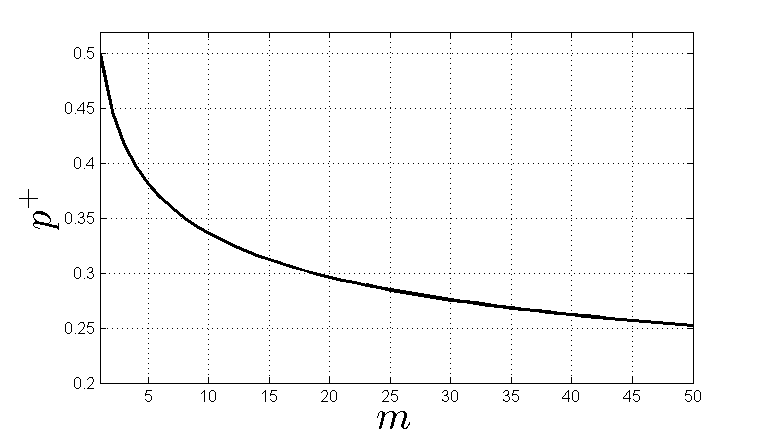
The term $p^{+}$ is plotted in Fig. 6 as a $m$ increases from $1$ to $50$ . Investigating this figure we see that $p^{+}$ equals to $0.5$ when $m=1$ which coincides with the bound for the exponent of polar codes presented by Arıkan and Telatar in [3]. As $m$ increases from $1$ to $50$ , $p^{+}$ and thus the achievable exponent decreases. The decrease is more steep for small values of $m$ and it becomes more monotone as $m$ increases.

In order to fully characterize the asymptotic performance of $\{\mathscr{C}_{n}^{(m)}\}$ one needs to provide a converse bound on $\beta$ which may be a difficult task. We believe that for the case $m>1$ , the achievable $\beta$ for $\{\mathscr{C}_{n}^{(m)}\}$ may show a dependency on the rate, $R\in[0,1]$ , chosen for the code; a phenomenon that does not exist when $m=1$ (see [10]). In order explain our conjecture, consider the process $\{\hat{Z}_{n}\}$ in (52) which we use to obtain an achievable bound on $\beta$ as $\beta<p^{+}$ . Our proof is based on the observation that once the realizations of $\hat{Z}_{n_{0}}$ are sufficiently close to $0$ , which happens with probability $I(W)$ , the scaling of $Z_{n}$ is mostly determined by the number of occurrences of state $+$ in $\{S_{n_{0}+1},S_{n_{0}+2},\ldots,S_{n}\}$ . From Theorem 2 we know that one typically observes $(n-n_{0})p^{+}$ occurrences of $+$ in $\{S_{n_{0}+1},S_{n_{0}+2},\ldots,S_{n}\}$ , therefore the value of $\log Z_{n}$ decreases $(n-n_{0})p^{+}$ times with the same speed as the code-length, $\log\hat{Z}_{n}=\log\hat{Z}_{n-1}+\log\hat{Z}_{n-m}$ , scaling as $\log Z_{n}=-\phi^{(n-n_{0})p^{+}}=-\phi^{n(1-\epsilon)p^{+}}$ . This result in the achievable exponent $\beta<p^{+}$ . However, when $m>1$ the value of $\log\hat{Z}_{n}$ may also decrease with a faster rate compared to that of the code-length. To see this, consider the case $(S_{n-1},S_{n-2},\ldots,S_{n-(m-1)})=(\bigstar,\bigstar,\ldots,\bigstar)\}$ and $S_{n}=+$ , where we have $\hat{Z}_{n-1}=\hat{Z}_{n-2}=\ldots=\hat{Z}_{n-(m-1)}$ and $\log\hat{Z}_{n}=\log\hat{Z}_{n-1}+\log\hat{Z}_{n-m}=\log\hat{Z}_{n-1}^{2}$ . Therefore, there may be times where $\log Z_{n}$ decreases with a faster rate as $\log\hat{Z}_{n}=\log Z_{n-1}^{2}$ instead of $\log\hat{Z}_{n}=\log\hat{Z}_{n-1}+\log\hat{Z}_{n-m}$ and this may result in a higher achievable $\beta$ . In order to quantify this we need to know not only the number of times state $+$ occurs in $\{S_{n}\}$ , but also the number of times a state $+$ in $\{S_{n}\}$ is preceded by $\bigstar$ states. Therefore, we need to refine Theorem 2 in terms of the number of transitions between states $+$ , $-$ and $\bigstar$ , as well. This might be a difficult but important problem whose solution will provide a full characterization of the asymptotic polarization performance of $\{\mathscr{C}_{n}^{(m)}\}$ and we leave it as a future work.

Refer to caption — Fig. 6: Achievable exponent, $\beta<p^{+}$ , as scaled with $m$ .

V Complexity and Sparsity

V-A Encoding and Decoding Complexity

We consider a single core processor with random access memory and investigate the time complexity of encoding and decoding of $\{\mathscr{C}_{n}^{(m)}\}$ . Let $\chi_{n}^{E}$ denote the complexity for encoding the information vector $\textbf{u}_{N}$ to encoded bits $\textbf{x}_{N}$ . We take complexity of each XOR operation as $1$ unit. By inspection of Fig 1, we have

\displaystyle\chi_{n}^{E}=\chi_{n-1}^{E}+\chi_{n-m}^{E}+N_{n-m}\quad n,m\geq 1,

(54)

where $\chi_{1}^{E}=1$ and $\chi_{0}^{E}=\chi_{-1}^{E}=\ldots=\chi_{1-m}^{E}=0$ .

Similarly, let $\chi_{n}^{D}$ denote the complexity for decoding the inputs of $W_{n}^{(i)}$ channels, where SCD is the decoding method. We take the complexity of computing the LR. relations in (34) as $1$ unit. We observe that one does not make any operations to calculate the LR in (35). By inspection of Fig 1, we have

\displaystyle\chi_{n}^{D}=\chi_{n-1}^{D}+\chi_{n-m}^{D}+2N_{n-m}\quad n,m\geq 1,

(55)

where $\chi_{0}^{D}=\chi_{-1}^{D}=\ldots=\chi_{1-m}^{D}=0$ .

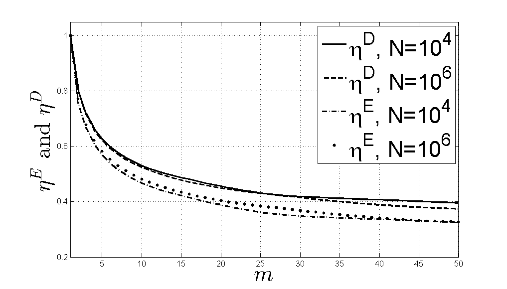
The recursions in (54) and (55) are cumbersome to deal with. To observe the scaling behavior of $\chi_{n}^{E}$ and $\chi_{n}^{D}$ in $m$ , we define

\displaystyle\eta^{E}\stackrel{{\scriptstyle\Delta}}{{=}}\frac{\chi_{n}^{E}}{N\log N},\quad\eta^{D}\stackrel{{\scriptstyle\Delta}}{{=}}\frac{\chi_{n}^{D}}{N\log N},

(56)

and demonstrate the scaling of $\eta^{E}$ and $\eta^{D}$ in Fig .7, where we have numerically calculated $\chi_{n}^{E}$ and $\chi_{n}^{D}$ as in (54) and (55) by choosing $N=O(\phi^{n})$ to be the code-length closest to $10^{4}$ and $10^{6}$ . From Fig. 7 we observe that, there exist a decrease in $\eta_{n}^{E}$ and $\eta_{n}^{D}$ as $m$ increases, where the decrease is more steep for small values of $m$ and it becomes more monotone as $m$ increases. This decrease in complexity, although not being orders of magnitude, is promising in showing the existence of polar codes requiring lower complexity. For example, from Fig. 7 we observe that $\eta_{n}^{D}$ is around $1/2$ when $m=12$ . This indicates that the decoding complexity of $\{{\mathscr{C}}_{n}^{(12)}\}$ is reduced by half compared to $\{{\mathscr{C}}_{n}^{(1)}\}$ which is the polar code presented by Arıkan in [1].

V-B Sparsity

As we have explained in Section II, there exist a sparsity in the channel combining process in the sense that at each combining level, the vector channel $W_{n}$ is obtained by combining $W_{n-1}$ and $\hat{W}_{n-m}$ which are obtained from $N(n-1)$ and $N(n-m)$ uses of underlying B-DMC, $W$ , respectively. From Proposition 5 we observe that the overall effect of channel combining and splitting is that, at each level $n$ , there exist $N(n-m)$ bit-channel pairs that participate in $\boxplus$ and $\boxminus$ transforms. As $m$ increases $N(n-m)$ decreases with respect to $N(n-1)$ implying the fraction of bit-channels participating in $\boxplus$ and $\boxminus$ transforms also decreases. On the other hand, as $m$ increases, the code-length increases less rapidly in $n$ because $N=O(\phi^{n})$ and $\phi$ is decreasing in $m$ , thus one can fit more channel combining and splitting levels within fixed code-length. A natural question is to understand the overall effect of increasing $m$ on the total number of $\boxplus$ and $\boxminus$ transforms that one can obtain when the number of uses of $W$ channels is fixed. The importance of $\chi_{n}^{D}$ in (55) comes to play at this point because it gives us the total number of $\boxplus$ and $\boxminus$ transformation that are recursively applied to independent uses of $W$ channels to obtain the bit-channels in $W_{n}$ . Consequently, one can view $\eta_{D}$ as a packing ratio in the sense that one can pack $\eta_{n}^{D}{N\log N}$ recursive applications of $\boxplus$ and $\boxminus$ transformation to $N$ independent uses of $W$ . Inspecting the scaling of $\eta_{D}$ in Fig. 7 we observe that this packing ratio is $1$ when $m=1$ and it decreases with increasing $m$ , and this decrease manifests itself as a reduction in the decoding complexity of $\{{\mathscr{C}}_{n}^{(m)}\}$ .

VI Conclusion and Future Work

We have introduced a method to design a class of code sequences $\{{\mathscr{C}}_{n}^{(m)};n\geq 1,m\geq 1\}$ with code-length $N=O(\phi^{n}),\phi\in(1,2],$ and memory order $m$ . The design of $\{{\mathscr{C}}_{n}^{(m)}\}$ is based on the channel polarization idea of Arıkan [1] and $\{{\mathscr{C}}_{n}^{(m)}\}$ coincides with the polar codes presented by Arıkan when $m=1$ . We showed that $\{{\mathscr{C}}_{n}^{(m)}\}$ achieves the symmetric capacity of arbitrary BDMCs for arbitrary but fixed $m$ . We have obtained an achievable bound on the asymptotic polarization of performance of $\{{\mathscr{C}}_{n}^{(m)}\}$ as scaled with $m$ and showed that the encoding and decoding complexities of $\{{\mathscr{C}}_{n}^{(m)}\}$ decrease with increasing $m$ . Our introduction of $\{{\mathscr{C}}_{n}^{(m)}\}$ complements Arıkan’s conjecture that channel polarization is a general phenomenon and it shows the existence of polar codes requiring lower complexity. Future work will include a rate dependent analysis and a converse result on the asymptotic polarization performance of $\{{\mathscr{C}}_{n}^{(m)}\}$ .

References

[1] E. Arıkan, “Channel Polarization: A Method for Constructing Capacity-Achieving Codes for Symmetric Binary-Input Memoryless Channels,” IEEE Trans. Inform. Theory, vol. 55, no. 7, pp. 3051–3073, Jul 2009.
[2] ——, “Channel combining and splitting for cutoff rate improvement,” IEEE Trans. Inform. Theory, vol. 52, no. 2, pp. 628–639, 2006.
[3] E. Arıkan and I. Telatar, “On the rate of channel polarization,” in Proc. IEEE Int. Symp. Inform. Theory (ISIT), 2009, pp. 1493–1495.
[4] S. Korada, E. Şaşoğlu, and R. Urbanke, “Polar codes: Characterization of exponent, bounds, and constructions,” IEEE Trans. Inform. Theory, vol. 56, no. 12, pp. 6253–6264, 2010.
[5] I. Tal and A. Vardy, “How to construct polar codes,” IEEE Trans. Inform. Theory, vol. 59, no. 10, pp. 6562–6582, Oct 2013.
[6] R. G. Bartle, The Elements of Real Analysis, 2nd. ed. John Wiley & Sons, 1995.
[7] P. Billingsley, Probability and Measure, 3rd. ed. John Wiley & Sons, 1927.
[8] T. Cover and J. Thomas, Elements of Information Theory. Wiley, 2005.
[9] H. Afşer and H. Deliç, “On the channel-specific construction of polar codes,” IEEE Comm. Letters, accepted, 2015.
[10] S. Hassani and R. Urbanke, “On the scaling of polar codes: I. the behavior of polarized channels,” in Proc. IEEE Int. Symp. Inform. Theory (ISIT), 2010, pp. 874–878.

VII Appendix

VII-A Proof of Proposition 1

We have $J(W^{-})=\frac{2}{1+Z(W^{-})}$ and $J(W^{+})=\frac{2}{1+Z(W^{+})}$ . By using (17) and (16) we obtain

		$\displaystyle J(W^{+})+J(W^{-})\geq\log\frac{2}{1+Z(W^{\prime})Z(W^{\prime\prime})}+$
		$\displaystyle\log\frac{2}{1+Z(W^{\prime})+Z(W^{\prime\prime})-Z(W^{\prime})Z(W^{\prime\prime})}$		(57)
		$\displaystyle\!\!\!=\log\frac{2}{1\!\!+\!\!Z(W^{\prime})\!\!+\!\!Z(W^{\prime\prime})+w(W^{\prime},W^{\prime\prime})Z(W^{\prime})Z(W^{\prime\prime})}$

where $w(W^{\prime},W^{\prime\prime})=Z(W^{\prime})+Z(W^{\prime\prime})-Z(W^{\prime})Z(W^{\prime\prime})\leq 1$ indicating

		$\displaystyle\!\!\!\!\!\!J(W^{+})+\!J(W^{-})\!\geq\!\log\frac{2}{1+Z(W^{\prime})}\!+\!\log\frac{2}{1+Z(W^{\prime\prime})}$		(58)
		$\displaystyle=J(W^{\prime})+J(W^{\prime\prime}).$

In order to have $J(W^{+})+J(W^{-})=J(W^{\prime})+J(W^{\prime\prime})$ , the equalities in (57) and (58) must be achieved. From (17) we know that the equality in (57) is achieved only if $Z(W^{\prime})\in\{0,1\}$ or $Z(W^{\prime\prime})\in\{0,1\}$ or if $W^{\prime}$ and $W^{\prime\prime}$ are BECs. When $(Z(W^{\prime}),Z(W^{\prime\prime}))\in(0,1)^{2}$ we have $w(W^{\prime},W^{\prime\prime})<1$ and the inequality in (58) is always strict, whether or not $W^{\prime}$ and $W^{\prime\prime}$ being BECs. Consider the case $Z(W^{\prime})=1$ or $Z(W^{\prime\prime})=1$ , then we have $w(W^{\prime},W^{\prime\prime})=1$ and the equalities in (57) and (58) are achieved. When $Z(W^{\prime})=0$ we have $J(W^{\prime})=1$ , $w(W^{\prime},W^{\prime\prime})=0$ and $J(W^{+})+J(W^{-})=J(W^{\prime})+J(W^{\prime\prime})$ , and the case $J(W^{\prime})=1$ follows from the symmetry in (57) and (58). Hence the equalities in (57) and (58) are both achieved only if $Z(W^{\prime})\in\{0,1\}$ or $Z(W^{\prime\prime})\in\{0,1\}$ , or alternatively only if $J(W^{\prime})\in\{0,1\}$ or $J(W^{\prime\prime})\in\{0,1\}$ .

VII-B Proof of Proposition 3

From the operation of $\varphi_{n}$ in Defn. 1 we obtain ${\cal S}_{1}=\{+,-\}$ such that $\textbf{s}_{1}^{(1)}=(+)$ and $\textbf{s}_{1}^{(2)}=(-)$ , indicating $\textbf{s}_{1}^{(1)}$ and $\textbf{s}_{1}^{(2)}$ are unique. Proof is by induction, assume that $s_{n-1}^{(j)}\in{\cal S}_{n-1}$ are unique. Let $j\in\mathbb{N}_{n-m}$ and consider $\textbf{s}_{n-1}^{(j)}$ to whom by appending $+$ and $-$ one obtains $\textbf{s}_{n}^{(j)}$ and $\textbf{s}_{n}^{(j+N(n-1))}$ , respectively, indicating $\textbf{s}_{n}^{(j+N(n-1))}$ and $\textbf{s}_{n}^{(j)}$ are different from each other. Next, let $j\in\mathbb{N}_{n-1}\setminus\mathbb{N}_{n-m}$ then $\textbf{s}_{n}^{(j)}$ are obtained by appending $\bigstar$ to $\textbf{s}_{n-1}^{(j)}$ which, by assumption, are unique. Combining the result we see that for all $j\in\mathbb{N}_{n}$ the vectors $s_{n}^{(j)}\in{\cal S}_{n}$ are different from each other.

VII-C Proof of Proposition 4

Investigating Fig 2 consider the operation of $\varphi_{n-1}$ where $s_{n-2}^{(k)}=(s_{1},s_{2},\ldots,s_{n-2})$ , $k\in\mathbb{N}_{n-2}$ , holds at level $n-1$ . Next, consider the operation of $\varphi_{n-2}$ where one has $s_{n-3}^{(k)}=(s_{1},s_{2},\ldots,s_{n-3})$ for $k\in\mathbb{N}_{n-3}$ . In turn and by induction through $\varphi_{n-2},\varphi_{n-3},\ldots,\varphi_{n-(m-1)}$ we conclude that $s_{n-m}^{(j)}=(s_{1},s_{2},\ldots,s_{n-m})$ , $j\in\mathbb{N}_{n-m}$ .

VII-D Proof of Proposition 6

i) For $m>1$ we have $F(m,1)=-1<0$ and $F(m,2)=2^{m-1}-1\geq 0$ so that there exists at least one real root in (1,2]. Proof is by contradiction, let $\rho_{1},\rho_{2}\in(1,2]$ be two real roots of $F(m,\rho)$ then from (37) we have

	$\displaystyle{\rho}_{1}^{m-1}(\rho_{1}-1)=1,$		(59)
	$\displaystyle{\rho}_{2}^{m-1}(\rho_{2}-1)=1.$		(60)

Let $\rho_{1}<\rho_{2}$ , then $\rho_{2}^{m-1}>{\rho}_{1}^{m-1}$ and $\rho_{2}-1>\rho_{1}-1>0$ implying ${\rho}_{2}^{m-1}({\rho}_{2}-1)>1$ if ${\rho}_{1}^{m-1}(\rho_{1}-1)=1$ which contradicts (60), carrying a similar analysis for $\rho_{1}<\rho_{2}$ also contradicts (60), which indicates $\rho_{1}=\rho_{2}=\phi$ .

ii) Assume that $\rho$ is a complex root of $F(m,\rho)$ , with $\sqrt{\rho\rho^{*}}=\sigma>1$ where $*$ denotes the conjugate operation. Since the coefficients of $F(m,\rho)$ are real, its complex roots must be in conjugate pairs. From (37)

	$\displaystyle\rho^{m-1}(\rho-1)=1,$
	$\displaystyle{\rho^{}}^{m-1}(\rho^{}-1)=1.$

Multiplying the above equations we obtain

	$\displaystyle\sigma^{2(m-1)}(\sigma^{2}-2Re(\rho)+1)=1,$
	$\displaystyle\sigma^{2(m-1)}(\sigma^{2}-2\sigma\alpha+1)=1,$		(61)

where $0\leq\alpha<1$ . In turn for any $\rho$ , $\sigma$ must be a root of

\displaystyle g(\sigma,\alpha)=\sigma^{2(m-1)}(\sigma^{2}-2\sigma\alpha+1)-1,

(62)

Observe that when $\sigma$ is fixed $g(\sigma,\alpha)$ is decreasing in $\alpha$ . We also have

\displaystyle\begin{split}\frac{\partial g(\sigma,\alpha)}{\partial\sigma}&={2(m-1)}\sigma^{2(m-1)-1}(\sigma^{2}-2\sigma\alpha+1)\\ &\quad+\sigma^{2(m-1)}(2\sigma-2\alpha)\end{split}

From (61) observe that $(\sigma^{2}-2\sigma\alpha+1)>0$ , and since $(2\sigma-2\alpha)>0$ for $\sigma>1$ we have $\frac{\partial g(\sigma,\alpha)}{\partial\sigma}>0$ . This indicates that $g(\sigma,\alpha)$ is increasing with $\sigma$ . But $\phi$ is a root of $g(\sigma,\alpha)$ with $\alpha=1$ and thus $g(\phi,1)=0$ . Since $g(\sigma,\alpha)$ is decreasing in $\alpha$ we have $g(\phi,\alpha)\geq 0$ and $g(\sigma,\alpha)=0$ is only achieved if $\sigma<\phi$ because $g(\sigma,\alpha)$ is increasing with $\sigma$ .

iii) Observe that for some $\rho\in(1,2]$ we have $\frac{\partial F(m,\rho)}{\partial\rho}>0$ so that $F(m,\rho)$ is increasing in $\rho$ and when $\rho$ is fixed $F(m,\rho)$ is also increasing in $m$ . Assume that $\rho_{1},\rho_{2}\in(1,2]$ are real roots of $F(m_{1},\rho)$ and $F(m_{2},\rho)$ , respectively, where $m_{1},m_{2}\geq 1$ . Then $f(m_{1},\rho_{1})<f(m_{2},\rho_{1})$ holds if $m_{2}>m_{1}$ and $f(m_{1},\rho_{1})=f(m_{2},\rho_{2})=0$ is satisfied only if $\rho_{1}<\rho_{2}$ .

VII-E Proof of Lemma 1

Let $J_{n}^{(i)}=J(W_{n}^{(i)})$ denote symmetric cut-off rate of $W_{n}^{(i)}$ . From Proposition 5 we know that for $j\in\mathbb{N}_{n-m}$ we have $W_{n}^{(j)}=W_{n-1}^{(j)}\boxplus W_{n-m}^{(j)}$ and $W_{n}^{(j+N(n-1))}=W_{n-1}^{(j)}\boxminus W_{n-m}^{(j)}$ . Proposition 1 indicates that these transforms increase the sum cut-off rate as $J_{n}^{(j)}+J_{n}^{(j+N(n-1))}\geq J_{n-1}^{(j)}+J_{n-1}^{(j)}$ where the equality is achieved only if $J_{n-1}^{(j)}\in\{0,1\}$ or $J_{n-m}^{(j)}\in\{0,1\}$ holds. For $j\in\mathbb{N}_{n-1}\setminus\mathbb{N}_{n-m}$ , from Proposition 5, we have $J_{n}^{(j)}=\gamma(n)J_{n-1}^{(j)}$ which implies $J_{n}^{(j)}=J_{n-1}^{(j)}$ . Combining the above results gives

\displaystyle\sum_{i\in\mathbb{N}_{n}}J_{n}^{(i)}\geq\sum_{j\in\mathbb{N}_{n-1}}J_{n}^{(j)}+\sum_{k\in\mathbb{N}_{n-m}}J_{n}^{(k)},

where the equality is achieved only of if $J_{n-1}^{(j)}\in\{0,1\}$ or $J_{n-m}^{(j)}\in\{0,1\}$ holds for all $j\in\mathbb{N}_{n-m}$ . In the probabilistic domain of SectionIV the above result is equivalent to

\displaystyle\sum_{\textbf{s}_{n}\in{\cal S}_{n}}J_{n}\geq\sum_{\textbf{s}_{n-1}\in{\cal S}_{n-1}}J_{n-1}+\sum_{\textbf{s}_{n-m}\in{\cal S}_{n-m}}J_{n-m},

where the equality is achieved only of if $J_{n-1}\in\{0,1\}$ or $J_{n-m}\in\{0,1\}$ holds for all $S_{n}\in\{+,-\}$ . Dividing both sides of the above inequality by $1/N(n)$ and using $E[J_{n}]=\frac{1}{N(n)}\sum_{\textbf{s}_{n}\in{\cal S}_{n}}J_{n}$ we obtain

\displaystyle E[J_{n}]\geq\frac{N(n-1)}{N(n)}E[J_{n-1}]+\frac{N(n-m)}{N(n)}E[J_{n-m}].

Noticing $\frac{N(n-1)}{N(n)}=\mu(n)$ and $\frac{N(n-m)}{N(n)}=1-\mu(n)$ completes the proof.

VII-F Proof of Lemma 2

From (40) we have

	$\displaystyle E[J_{n}]\geq\mu E[J_{n-1}]+\left(1-\mu\right)E[J_{n-m}],$
	$\displaystyle\geq\min\{E[J_{n-1}],E[J_{n-m}]\},$		(63)

Let us define the set

\displaystyle{\cal E}_{k}^{(m)}\stackrel{{\scriptstyle\Delta}}{{=}}\{E_{km},E_{km-1},\ldots,E_{km-(m-1)}\}.

By definition in (41) we have we have $E[\hat{J}_{k}]=\min{\cal E}_{k}^{(m)}$ . Proof is by induction. We use (63) to upper bound the elements of ${\cal E}_{k}^{(m)}$ with respect to $\min{\cal E}_{k-1}^{(m)}=E[\hat{J}_{k-1}]$ . Let $n=km-(m-1)$ and use (63) to obtain

	$\displaystyle E_{km-(m-1)}$	$\displaystyle\geq\min\{E_{(k-1)m},E_{(k-1)m-(m-1)}\},$
		$\displaystyle\geq\min{\cal E}_{k-1}^{(m)}$

For $i=2,3,\ldots,m-1$ assume

\displaystyle E_{km-(m-i)}\geq\min{\cal E}_{k-1}^{(m)}

holds. Next, let $n=km-(m-(i+1))$ in (63) to write

\displaystyle E_{km-(m-(i+1))}

\displaystyle\geq\min\{E_{km-(m-i)},E_{(k-1)m-(m-(i+1))}\}.

By assumption $E_{km-(m-i)}\geq\min{\cal E}_{k-1}^{(m)}$ and by definition $E_{(k-1)m-(m-(i+1))}\geq\min{\cal E}_{k-1}^{(m)}$ holds, indicating

\displaystyle E_{km-(m-(i+1))}

\displaystyle\geq\min{\cal E}_{k-1}^{(m)}.

Combining the above results tells us for $i=1,2,\ldots,m$ we have $E_{km-(m-i)}\geq\min{\cal E}_{k-1}^{(m)}=E[\hat{J}_{k-1}]$ which indicates $E[\hat{J}_{k}]\geq E[\hat{J}_{k-1}]$ .

VII-G Proof of Lemma 3

In order to bound $|{\cal T}_{n}^{(q)}|$ we decompose ${\cal T}_{n}^{(q)}$ it into two different sets

	$\displaystyle{\cal T}_{n}^{(a,q)}$	$\displaystyle\stackrel{{\scriptstyle\Delta}}{{=}}\left\{\textbf{s}^{n}:P_{\textbf{s}^{n}}^{(\mathord{-})}=q,s_{n}=+\right\},$
	$\displaystyle{\cal T}_{n}^{(b,q)}$	$\displaystyle\stackrel{{\scriptstyle\Delta}}{{=}}\left\{\textbf{s}^{n}:P_{\textbf{s}^{n}}^{(\mathord{-})}=q,s_{n}\neq+\right\}$

and we have $T_{n}^{(q)}={\cal T}_{n}^{(a,q)}\cup{\cal T}_{n}^{(b,q)}$ . Recall that each state $-$ in $\textbf{s}_{n}$ is followed by $m-1$ occurrences of state $\bigstar$ . In turn, ${\cal T}_{n}^{(a,q)}$ consists of $\textbf{s}_{n}$ having $k=nq$ , $0\leq k\leq n/m$ , occurrences of the vector $\textbf{a}=(-,\underbrace{\bigstar,\bigstar,\ldots,\bigstar}_{m-1\text{ times}})$ and $n-km$ occurrences of state $+$ . By combinatorial analysis we have

\displaystyle|{\cal T}_{n}^{(a,q)}|={n-(m-1)k\choose k}.

${\cal T}_{n}^{(b,q)}$ consists of $k-1$ occurrences of the vector a, an occurrence of $\textbf{b}=(-,\underbrace{0,0,\ldots,0}_{p\text{ times}})$ , $1\leq p<m-1$ , and $n-mk-(p+1)$ occurrences of state $+$ . The vector b can only occur in the last $p+1$ entries in $\textbf{s}_{n}$ and it will be completed to a vector a if we had prolonged the channel combining operation $m-1-p\leq m$ more levels. Therefore

\displaystyle|{\cal T}_{n}^{(b,q)}|

\displaystyle\leq{n+m-(m-1)k\choose k}.

For some $c\in\mathbb{Z}$ and $d\in\mathbb{Z}$ with $c<d$ we have ${d\choose c}=\frac{d}{d-c}{d-1\choose c}\leq d{d-1\choose c}$ , using this fact we obtain

	$\displaystyle{n+m-(m-1)k\choose k}$	$\displaystyle\leq(n+m){n+(m-1)-(m-1)k\choose k},$
		$\displaystyle<(n+m)^{2}{n+(m-2)-(m-1)k\choose k}$
		$\displaystyle\quad\quad\vdots$
		$\displaystyle<(n+m)^{m}{n-(m-1)k\choose k}$

Then we have

$\displaystyle\|{\cal T}_{n}^{(q)}\|$	$\displaystyle=\|{\cal T}_{n}^{(a,q)}\|+\|{\cal T}_{n}^{(b,q)}\|,$
	$\displaystyle<\left(1+(n+m)^{m}\right){n-(m-1)k\choose k},$
	$\displaystyle<\left(1+(n+m)\right)^{m}{n-(m-1)k\choose k},$
	$\displaystyle=2^{nB(m,n)}{n-(m-1)k\choose k},$	(64)

where $B(m,n)=\frac{m\log(1+n+m)}{n}=o(1)$ . Next, we use the upper bound ${n\choose k}\leq 2^{nH(k/n)}$ in [8] to upper bound ${n-(m-1)k\choose k}$ as

	$\displaystyle{n-(m-1)k\choose k}$	$\displaystyle\leq 2^{n(1-(m-1)(k/n))H(\frac{(k/n)}{1-(m-1)(k/n)}},$
		$\displaystyle=2^{nG(m,q)}.$		(65)

Combining (64) and (65)we obtain the desired bound as $|T_{n}^{(q)}|<2^{n(G(m,q)+B(m,n))}=2^{n(G(m,q)+o(1))}$ .

VII-H Proof of Lemma 4

We have

\displaystyle G(m,q)=(1-(m-1)q)H\left(\frac{(q)}{1-(m-1)q}\right).

We know that, for $q\in[0,1/m]$ , $H(\frac{q}{1-(m-1)q})$ is concave in $q$ and $(1-(m-1)q)$ is linear in $q$ indicating $G(m,q)$ is concave in $q$ . Let $q*$ denote the maximizer of $G(m,q)$ . The maximum of $H(\frac{q}{1-(m-1)q})$ occurs when $\frac{q}{1-(m-1)q}=\frac{1}{2}$ or equivalently when $q=\frac{1}{m+1}$ and since $(1-(m-1)q)$ is decreasing in $q$ , we have $q*\in[0,\frac{1}{m+1}]$ . We next evaluate $\frac{\partial G(m,q)}{\partial q}$

\displaystyle\begin{split}\frac{\partial G(m,q)}{\partial q}&=(m-1)\log(1-(m-1)q)\\ &\quad\quad+\log q-m\log(1-mq).\end{split}

setting $\frac{\partial G(m,q)}{\partial q}|_{q=q*}=0$ gives

\displaystyle\!\!\!\!\!\!(m-1)\log(1-(m-1)q^{*})+\!\!\log q^{*}=m\log(1-mq^{*}).

(66)

Re-arranging the above equation we obtain

\displaystyle\begin{split}&m\log\frac{(1-(m-1)q^{*})}{1-mq^{*}}+\log\frac{q^{*}}{1-mq^{*}}\\ &\quad=\log\frac{(1-(m-1)q^{*})}{1-mq^{*}}.\end{split}

(67)

Let us use the following substitutions

\displaystyle\eta=\frac{1-(m-1)q^{*}}{1-mq^{*}},\quad\eta-1=\frac{q^{*}}{1-mq^{*}}.

For $q*\in[0,\frac{1}{m+1}]$ we have $\eta\in[1,2]$ . Using the above substitutions in (67) we obtain

\displaystyle m\log\eta+\log(\eta-1)=\log\eta,

or alternatively

\displaystyle\eta^{m}(\eta-1)=\eta.

Dividing both sides of the above relation by $\eta$ and re-arranging the terms we obtain

\displaystyle\eta^{m}-\eta^{m-1}-1=0.

(68)

But the above polynomial is same as 37. Consequently from part i of Proposition. 6 we conclude that $\eta=\phi$ which indicates that $\frac{1-(m-1)q^{*}}{1-mq^{*}}=\phi$ and hence $q^{*}=\frac{1}{1+m(\phi-1)}=p^{-}$ . Next we evaluate the maximum of $G(m,q)$ attained at $q=q^{*}$ .

	$\displaystyle G(m,q^{})=-q^{}\log\frac{q^{}}{1-(m-1)q^{}}+$
	$\displaystyle(mq^{}-1)\log\frac{1-mq^{}}{1-(m-1)q^{*}}\quad$		(69)

Re-arranging (66) we observe that

\displaystyle\log\frac{q^{*}}{1-(m-1)q^{*}}=m\log\frac{1-mq^{*}}{1-(m-1)q^{*}}

Using the above relation in (69) gives

\displaystyle G(m,q^{*})=\log\frac{1-(m-1)q^{*}}{1-mq^{*}}=\log\phi.

VII-I Proof of Proposition 8

We define a typical set ${\cal T}_{n}^{(q,\epsilon)}$ as

\displaystyle{\cal T}_{n}^{(q,\epsilon)}=\{\textbf{s}_{n}:P_{s^{n}}^{(-)}=q,D(q,p^{-})\leq\epsilon\}.

The probability that ${\cal T}_{n}^{(q)}$ is not typical is

$\displaystyle 1-\Pr({\cal T}_{n}^{(q,\epsilon)})$	$\displaystyle=\sum_{\Pr(D(q,p^{-})>\epsilon)}\Pr({\cal T}_{n}^{(q)}),$
	$\displaystyle\stackrel{{\scriptstyle a}}{{\leq}}\sum_{\Pr(D(q,p^{-})>\epsilon)}2^{-n\left(D(q,s_{-})+o(1)\right)},$
	$\displaystyle\stackrel{{\scriptstyle}}{{\leq}}\sum_{\Pr(D(q,p^{-})>\epsilon)}2^{-n\left(\epsilon+o(1)\right)},$
	$\displaystyle\stackrel{{\scriptstyle b}}{{\leq}}(n+1)2^{-n\left(\epsilon+o(1)\right)},$
	$\displaystyle=2^{-n\left(\epsilon+o(1)\right)},$	(70)

In the above derivation (a) follows from (49) and (b) follows from the fact that there exist at most $n+1$ different type classes having $\Pr(D(q,s_{-})>\epsilon)$ . The above result indicates that $\sum_{n\rightarrow\infty}\Pr(D(q,s_{-})\geq\epsilon)$ converges, thus the expected number of the occurrences of the event $D(q,s_{-})>\epsilon$ for all $n$ is finite. By using the first Borel Cantelli Lemma [7, p. 59] we conclude that $D(q,s_{-})$ converges to $0$ with probability 1.

VII-J Proof of Lemma 5

Conditioned on the event $D_{n_{0}}^{n}(\gamma)=\#\big((s_{n_{0}+1},\ldots,s_{n})|+\big)\geq\gamma(n-n_{0})$ there exists at least $\gamma(n-n_{0})$ occurrences of state $+$ in $\{S_{n_{0}+1},S_{n_{0}+2},\ldots,S_{n}\}$ . Investigating (52), we have $\hat{Z}_{n}\leq\hat{Z}_{n-1}$ when $S_{n}=+$ and $Z_{n}\geq Z_{n-1}$ when $S_{n}\neq+$ . Moreover, $Z_{n}$ is increasing in $Z_{n-1}$ when $S_{n}$ is fixed. Consequently, if we fix $\hat{Z}_{m}$ , the largest value of $\hat{Z}_{n}$ will occur if $\{S_{n_{0}+1},S_{n_{0}+2},\ldots\,S_{n}\}$ has the following realization

\displaystyle\{\!\!\!\!\!\!\!\overbrace{\textbf{a},\textbf{a},\ldots,\textbf{a},}^{(1-\gamma)(n-n_{0})/m\text{ times}}\!\!\!\!\!\!\!\!\underbrace{+,+,\ldots,+}_{\gamma(n-n_{0})\text{ times}}\}.

where $\textbf{a}=(-,\underbrace{\bigstar,\bigstar,\ldots,\bigstar}_{m-1\text{ times}})$ . In order to upper bound $\hat{Z_{n}}$ we assume that the above realization has occured for $\{S_{n_{0}+1},S_{n_{0}+2},\ldots\,S_{n}\}$ . During consecutive runs of $+$ , the value of $\log\hat{Z}_{n}$ increases with the same recursion as the code-length in (1) as $\log\hat{Z}_{n}=\log\hat{Z}_{n-1}+\log\hat{Z}_{n-m}$ . This recursion happens $\gamma(n-m)$ times and since the code-legth obeying the same recursion scales as $\phi^{\gamma(n-m)}$ , $\phi\in(1,2]$ , we have

\displaystyle\log\hat{Z}_{n}=\phi^{\gamma(n-n_{0})}\log\hat{Z}_{k},

(71)

where $k=n_{0}+(1-\gamma)(n-m)$ . During consecutive runs of a the value of $\hat{Z}_{i}$ does not change with respect to $\hat{Z}_{i-1}$ when $S_{i}=\bigstar$ and it increases as $\hat{Z}_{i}=\hat{Z}_{i-1}+\hat{Z}_{i-m}-\hat{Z}_{n-1}\hat{Z}_{i-m}$ when $S_{i}=-$ . By construction of $\{S_{n_{0}+1},S_{n_{0}+2},\ldots\,S_{n}\}$ each state $-$ is preceed by $m-1$ occurances of $\bigstar$ therefore if $S_{i}=-$ we have $(S_{i-1},S_{i-2},\ldots,S_{i-(m-1)})=(\bigstar,\bigstar,\ldots,\bigstar)$ indicating $\hat{Z}_{i-1}=\hat{Z}_{i-2}=\ldots=\hat{Z}_{i-(m-1)}$ . Therefore during each occurance of state $-$ in a we see the recursion $\hat{Z}_{i-1}+\hat{Z}_{i-m}-\hat{Z}_{i-1}\hat{Z}_{i-m}=2\hat{Z}_{i-1}-\hat{Z}_{i}^{(i)}$ or equvalently $1-\hat{Z}_{i}=(1-\hat{Z}_{i}^{(i)})^{2}$ . This recursion occurs $(1-\gamma)(n-n_{0})$ times resulting in $1-\hat{Z}_{k}=(1-\hat{Z}_{n_{0}})^{2(1-\gamma)(n-n_{0})}$ and $\hat{Z}_{k}=1-(1-\hat{Z}_{n_{0}})^{2(1-\gamma)(n-n_{0})}$ . Next, employ the inequality $\log x\leq x-1$ , $x\in[0,1]$ , by letting $x=\hat{Z}_{k}$ to obtain

\displaystyle\log\hat{Z}_{k}\leq-(1-\hat{Z}_{n_{0}})^{2(1-\gamma)(n-n_{0})}.

(72)

Using (72) in (71) gives

	$\displaystyle\log\hat{Z}_{n}$	$\displaystyle=-\phi^{\gamma(n-n_{0})}(1-Z_{n_{0}})^{2(1-\gamma)(n-n_{0})},$
		$\displaystyle\leq-\phi^{\gamma(n-n_{0})}(1-Z_{n_{0}})^{2(n-n_{0})}$
		$\displaystyle=-\phi^{(\gamma-\epsilon)(n-n_{0})}\left((1-Z_{n_{0}})^{2}\phi^{\epsilon}\right)^{(n-n_{0})}.$

Choose $\zeta\in(0,1)$ so that $\zeta\leq 1-\phi^{\frac{-\epsilon}{2}}$ holds. Conditioned on $C_{n_{0}}(\zeta)=\{Z_{n_{0}}\leq\zeta\}$ we have $(1-Z_{n_{0}})^{2}\phi^{\epsilon}\geq 1$ , resulting in

\displaystyle\log_{2}\hat{Z}_{n}\leq-\phi^{(\gamma-\epsilon)(n-m)},\quad C_{n_{0}}(\zeta)\cap D_{n_{0}}^{n}(\gamma),

which proves the lemma.

	$\displaystyle W^{-}(y_{1},y_{2}\|x_{1})$	$\displaystyle=\sum_{x_{2}}\frac{1}{2}W^{\prime}(y_{1}\|x_{1}\oplus x_{2})W^{\prime\prime}(y_{2}\|x_{2}),$		(9)
	$\displaystyle W^{+}(y_{1},y_{2},x_{1}\|x_{2})$	$\displaystyle=\frac{1}{2}W^{\prime}(y_{1}\|x_{1}\oplus x_{2})W^{\prime\prime}(y_{2}\|x_{2}),$		(10)