跳到论文正文
W Papers独立论文阅读器 arXiv:1510.04044 论文正文 计算阅读时间 · 0%
引用这篇论文根据当前论文元数据生成,正式投稿前建议核对。


License: arXiv.org perpetual non-exclusive license
arXiv:1510.04044v3 [math.DS] 09 Apr 2019

Lyapunov Function Partial Differential Equations for Chemical Reaction Networks: Some Special CasesThanks: This work is supported by National Natural Science Foundation of China under Grant No. 11671418, 11271326 and 61611130124, and the Research Fund for the Doctoral Program of Higher Education of China under Grant No. 20130101110040.

Zhou Fang22footnotemark: 2    Chuanhou Gao22footnotemark: 2
Abstract

In this paper we develop a method to generate the Lyapunov function for stability analysis for chemical reaction networks. Based on the Chemical Master Equation, we derive the Lyapunov Function partial differential equations (PDEs), whose solution approximates the scaling non-equilibrium potential and serves as the candidate Lyapunov function for the given network. We further prove that for any chemical reaction network the solution (if exists) of the PDEs is dissipative. Moreover, the proposed method of Lyapunov Function PDEs is qualified for analyzing the asymptotic stability of complex balanced networks, all networks with 11-dimensional stoichiometric subspace and some special networks with more than 22-dimensional stoichiometric subspace if some moderate conditions are added. Several examples are presented to illustrate the efficiency of the method.

keywords
chemical reaction network, mass action system, Lyapunov Function PDEs, non-equilibrium potential, stability.
AMS
35F20, 37C10, 60J28, 80A30, 93D20

1 Introduction

Chemical reactions networks (CRNs) arise abundantly in the fields including chemistry, systems biology, process industry, and even those seemingly irrelevant to chemistry such as mechanics and ecology. The dynamics of a CRN often appears to be extremely complex due to chemical interactions of cellular processes but sometimes still exhibiting certain regular behaviors like period solutions and stable-fixed-points. As a special subclass, mass-action CRNs (CRNs assigned mass action kinetics, often named mass action systems) have the dynamics of the concentrations of the various species captured by polynomial ordinary differential equations (ODEs), and have received much attention since the pioneering work [10, 11, 12, 18] emerged. A major concern over this class of systems is to understand the relations between network structures and/or parameters and dynamical properties [7, 6, 28], especially in characterizing the stability (in the sense of Lyapunov) property [1, 2, 18, 29, 27, 24]. Following this line of study, we also focus on capturing stability of equilibria in mass action systems (MASs) in the current work. Naturally, Lyapunov functions are desirable objects to prove stability of equilibria. In the field of CRNs, one important example is the pseudo-Helmholtz free energy function, proposed by Horn and Jackson[18]. This Lyapunov function can be derived from the microscopic level using potential theory[2]. Here, we build further on this, and provide a general theory that bridges between the microscopic and the macroscopic level, thermodynamics and potential theory. Based on it, it is possible to derive or find a Lyapunov function for any MAS.

The early work on stability analysis mainly focused on exploring causal association from the network topology to the distribution of equilibria, and further to stability of equilibria. Thereinto, the weakly reversible structure, a requirement of complex balanced MAS, is the most active one. Horn et al.[18] proved the well-known Deficiency Zero Theorem that states a weakly reversible deficiency zero MAS to be complex balanced and to have only one equilibrium in each positive stoichiometric compatibility class. Moreover, each equilibrium in the complex balanced system is locally asymptotically stable, for which the pseudo-Helmholtz free energy function is proposed as the Lyapunov function. Feinberg[12] extended this theorem to the well-known Deficiency One Theorem that suggests a weakly reversible MAS to admit a sole equilibrium in each positive stoichiometric compatibility class if some required conditions on network deficiency (not necessary to be zero) are satisfied. Based on these results, the global asymptotical stability of equilibria in a complex balanced MAS was further obtained[26, 27] if the network is assumed to be persistent [11, 23, 8, 15], i.e., no stable boundary equilibrium if the initial point is in the interior of ℝ≥0n\mathbb{R}^{n}_{\geq 0}. Except for the weakly reversible structure, the reversible one, which acts as a special case of the former and is a requirement of detailed balanced MASs, is also the focus of attention. Feinberg [13] derived necessary and sufficient conditions, i.e., circuit conditions and spanning forest conditions, to say a reversible MAS to be detailed balanced. Recently, van der Schaft et al. [29] revisited this class of systems, and reported a compact formulation to describe the dynamics utilizing the graph theory (complex graph). The locally asymptotic stability of detailed balanced networks follows naturally from the fact that they are also complex balanced. Still, the pseudo-Helmholtz free energy function serves as the Lyapunov function.

An important means for stability analysis of a MAS is to construct a Lyapunov function according to the network structure. Although the pseudo-Helmholtz free energy function is capable for rendering asymptotical stability of MASs equipped with the weakly reversible or reversible structure, it fails to serve for those networks, like 3​S2⟶3​S1⟶2​S1+S23S_{2}\longrightarrow 3S_{1}\longrightarrow 2S_{1}+S_{2}, where S1S_{1} and S2S_{2} are the species. Clearly, this network is neither weakly reversible nor reversible. We name MASs with general structure (not necessarily weakly reversible or reversible) as balanced MASs if an equilibrium is admitted. For balanced MASs, Angeli and his coauthor [1] proposed Piecewise Linear in Rates Lyapunov Functions for stability analysis. The existence of such functions (they defined the networks having this attribute as 𝒫\mathscr{P} network set, which is actually a subset of balanced MASs) can guarantee stability of equilibrium, and further serves to establish asymptotical stability within the corresponding positive stoichiometric compatibility class if the Lyapunov function satisfies the LaSalle’s condition. Another possible solution to address the stability problem of a balanced MAS comes from the concept of realization presented by Szederkényi et. al. [28]. It is possible to find a complex balanced or detailed balanced realization for the network in question, then its asymptotical stability holds based on the dynamics equivalence between the network and its realization.

Different from all of the above investigations stemming from macroscopic deterministic analysis, some literature contributes to explaining the system properties from a microscopic stochastic viewpoint. Li and Yi [20, 21] connected the strength of attractions to the global attractor with the stationary distribution of a diffusion system, in which a white noise is added to the deterministic case. In the meanwhile, Anderson et. al. [2], starting from a Markov chain model, managed to design a Lyapunov function from a microscopic stochastic concept related to CRNs, termed as non-equilibrium potential that equals to the minus logarithm of stationary distribution of state. They proved that the scaling limit of non-equilibrium potential could act as a Lyapunov function for some MASs. Moreover, such a limit value coincides with the well-known pseudo-Helmholtz free energy function in the case of complex balanced MASs. This design thought is also valid for general birth-death MASs and some examples of non-complex and non-detailed balanced MASs. These encouraging results motivate us to find a Lyapunov function for MASs rooted in their microscopic concepts. In this paper, we take an approximation of the scaling non-equilibrium potential directly as a possible Lyapunov function and carry out this idea on Chemical Master Equation. A partial differential equation (PDE) is thus derived with the solutions serving as candidate Lyapunov functions. We have further proved the equation solutions dissipative, and able to serve as Lyapunov functions for complex balanced MASs, all networks with 11-dimensional stoichiometric subspace and some special networks with more than 22-dimensional stoichiometric subspace if some moderate conditions are added.

The remainder of this paper is organized as follows. Section 22 revisits some basic concepts about CRNs and the macroscopic deterministic dynamics of network derived from microscopic stochastic model. This is followed by the development of the Lyapunov Function PDEs in Section 33. Section 44 devotes to analyzing the property of solutions of the Lyapunov Function PDEs, and applications to complex balanced MASs. In Section 55, we discuss the validity of the Lyapunov Function PDEs for CRNs with 11-dimensional stoichiometric subspace, and further prove their efficacy in some special examples of CRNs with more than 22-dimensional stoichiometric subspace in Section 66. Finally, conclusions and a conjecture to say the validity of the Lyapunov Function PDEs to general balanced MASs are summarized in Section 77.  
 
Mathematical Notation:
 

  ℝn,ℝ≥0n,ℝ>0n\mathbb{R}^{n},\mathbb{R}^{n}_{\geq 0},\mathbb{R}^{n}_{\textgreater 0}

: nn-dimensional real space, nonnegative and positive real space, respectively.

  xv⋅ix^{v_{\cdot i}}

: xv⋅i=∏j=1dxjvj​ix^{v_{\cdot i}}=\prod_{j=1}^{d}x_{j}^{v_{ji}}, where x,v⋅i∈ℝdx,v_{\cdot i}\in\mathbb{R}^{d} and 000^{0} is defined to be 11.

  Ln⁡(x)\mathrm{Ln}(x)

: Ln⁡(x)=(ln⁡x1,ln⁡x2,⋯,ln⁡xd)⊤\mathrm{Ln}(x)=\left(\ln{x_{1}},\ln{x_{2}},\cdots,\ln{{x}_{d}}\right)^{\top}, where x∈ℝ>0dx\in\mathbb{R}^{d}_{>{0}}.

  ⊗\otimes

: Cartesian product.

  𝒞i\mathscr{C}^{i}

: The function set whose elements are ii-th continuous differentiable.

  0n\mathbbold{0}_{n}

: nn-dimensional vector with every entry to be zero.


2 Preliminary on CRNs

In this section, we will sketch some basic concepts about CRNs [14] and revisit the macroscopic dynamics of mass-action CRNs based on the microscopic analysis [2].

2.1 Basic Concepts

Consider a network with nn species, denoted by {S1,⋯,Sn}\{S_{1},\cdots,S_{n}\}, and rr chemical reactions with the iith reaction ℛi\mathcal{R}_{i} written as

Σj=1n​vj​i​Sj⟶Σj=1n​vj​i′​Sj,\Sigma_{j=1}^{n}v_{ji}S_{j}\longrightarrow\Sigma_{j=1}^{n}v^{\prime}_{ji}S_{j},

where v⋅iv_{\cdot i}, v⋅i′∈ℤ≥0nv^{\prime}_{\cdot i}\in\mathbb{Z}^{n}_{\geq 0} represent the complexes of reactant and resultant, respectively, of this reaction. Note that we label each reaction as a unidirectional reaction, here. If the iith reaction is reversible, the reverse reaction is naturally covered by exchanging v⋅iv_{\cdot i} and v⋅i′v^{\prime}_{\cdot i} in the reaction.

Based on the above information, some basic concepts about CRNs may be defined [14].

Definition 1 (Chemical Reaction Network).

Denote the finite sets of species, complexes and reactions by 𝒮={S1,S2,⋯,Sn}\mathcal{S}=\{S_{1},S_{2},\cdots,S_{n}\}, 𝒞=⋃i=1r{v⋅i,v⋅i′}\mathcal{C}=\bigcup_{i=1}^{r}\{v_{\cdot i},v^{\prime}_{\cdot i}\} and ℛ={v⋅1→v⋅1′,⋯,v⋅r→v⋅r′}\mathcal{R}=\{v_{\cdot 1}\to v^{\prime}_{\cdot 1},\cdots,v_{\cdot r}\to v^{\prime}_{\cdot r}\}, respectively, and Card⁡(𝒞)=c\mathrm{Card}(\mathcal{C})=c. If the following conditions hold


(i)\mathrm{(i)} There is no reaction v⋅i→v⋅i′∈ℛv_{\cdot i}\to v^{\prime}_{\cdot i}\in\mathcal{R} (i=1,⋯,ri=1,\cdots,r) such that v⋅i=v⋅i′v_{\cdot i}=v^{\prime}_{\cdot i};


(ii)\mathrm{(ii)} The jjth (j=1,⋯,n)(j=1,\cdots,n) entry of v⋅iv_{\cdot i} represents the stoichiometric coefficient of species Sj∈𝒮S_{j}\in\mathcal{S} in complex v⋅iv_{\cdot i},

then the triple (𝒮,𝒞,ℛ)(\mathcal{S},\mathcal{C},\mathcal{R}) is called a chemical reaction network.

Definition 2 (Stoichiometric Subspace).

For a CRN (𝒮,𝒞,ℛ)(\mathcal{S},\mathcal{C},\mathcal{R}), the linear subspace 𝒮=span⁡{v⋅1−v⋅1′,⋯,v⋅r−v⋅r′}\mathscr{S}=\mathrm{span}\{v_{\cdot 1}-v^{\prime}_{\cdot 1},\cdots,v_{\cdot r}-v^{\prime}_{\cdot r}\} is called the stoichiometric subspace of the network.

Definition 3 (Stoichiometric Compatibility Class).

Let 𝒮\mathscr{S} be the stoichiometric subspace of a CRN (𝒮,𝒞,ℛ)(\mathcal{S},\mathcal{C},\mathcal{R}) and C∈ℝ≥0nC\in\mathbb{R}^{n}_{\geq 0} be a nonnegative nn-dimensional vector, then C+𝒮={C+ξ|ξ∈𝒮}C+\mathscr{S}=\{C+\xi|\xi\in\mathscr{S}\} is a stoichiometric compatibility class of CC for the network; (C+𝒮)​⋂ℝ≥0n(C+\mathscr{S})\bigcap\mathbb{R}^{n}_{\geq 0} is a nonnegative stoichiometric compatibility class and (C+𝒮)​⋂ℝ>0n(C+\mathscr{S})\bigcap\mathbb{R}^{n}_{>0} is a positive stoichiometric compatibility class.

When a CRN is assigned a mass action kinetics, the rate for reaction v⋅i→v⋅i′v_{\cdot i}\to v^{\prime}_{\cdot i} is evaluated by ki​xv⋅ik_{i}x^{v_{\cdot i}}, where ki∈ℝ>0k_{i}\in\mathbb{R}_{\textgreater 0} is the rate constant for this reaction, x∈ℝ≥0nx\in\mathbb{R}^{n}_{\geq 0} is the vector of concentrations xjx_{j} of the chemical species Sj,j=1,⋯,nS_{j},~j=1,\cdots,n, and

xv⋅i:=∏j=1nxjvj​i.x^{v_{\cdot i}}:=\prod_{j=1}^{n}x_{j}^{v_{ji}}.
Definition 4 (Mass Action System).

Denote the set of reaction rate constants by 𝒦=(k1,⋯,kr)\mathcal{K}=(k_{1},\cdots,k_{r}) with kik_{i} representing the rate constant for reaction v⋅i→v′⋅i,i=1,⋯,rv_{\cdot i}\to v^{\prime}_{\cdot i},~i=1,\cdots,r. A CRN (𝒮,𝒞,ℛ)(\mathcal{S},\mathcal{C},\mathcal{R}) taken together with the set of reaction rate constants 𝒦\mathcal{K} is called a mass action system, referred to as (𝒮,𝒞,ℛ,𝒦)(\mathcal{S},\mathcal{C},\mathcal{R},\mathcal{K}).

The dynamics of a MAS (𝒮,𝒞,ℛ,𝒦)(\mathcal{S},\mathcal{C},\mathcal{R},\mathcal{K}) that captures the changes of concentrations of every species over time tt is thus expressed as

d​xd​t=Γ​R​(x),x∈ℝ≥0n,\frac{\text{d}x}{\text{d}t}=\varGamma R(x),\quad\quad x\in\mathbb{R}^{n}_{\geq 0}, (1)

where Γ∈ℤn×r\varGamma\in\mathbb{Z}_{n\times r} is the stoichiometric matrix, defined by Γ⋅i=v⋅i′−vi\varGamma_{\cdot i}=v^{\prime}_{\cdot i}-v_{i}, and R⁡(x)R(x) is rr-dimensional vector-valued function with Ri​(x)=ki​xv⋅iR_{i}(x)=k_{i}x^{v_{\cdot i}}.

Definition 5 (Balanced MAS).

For a MAS (𝒮,𝒞,ℛ,𝒦)(\mathcal{S},\mathcal{C},\mathcal{R},\mathcal{K}), a vector of concentrations x∗∈ℝ>0nx^{*}\in\mathbb{R}^{n}_{\textgreater 0} is called an equilibrium if its dynamical equation eq. 1 satisfies Γ​R​(x∗)=0\varGamma R(x^{*})=0. A MAS that admits an equilibrium is said to be a balanced MAS.

Definition 6 (Complex Balanced MAS).

For a MAS (𝒮,𝒞,ℛ,𝒦)(\mathcal{S},\mathcal{C},\mathcal{R},\mathcal{K}), a vector of concentrations x∗∈ℝ>0nx^{*}\in\mathbb{R}^{n}_{\textgreater 0} is called a complex balanced equilibrium if at this state the combined rate of outgoing reactions from any complex is equal to the combined rate of incoming reactions to it, i.e.

∑{i|v⋅i=z}ki​(x∗)v⋅i=∑{i|v⋅i′=z}ki​(x∗)v⋅i,∀z∈𝒞.{\sum_{\{i|v_{\cdot i}=z\}}k_{i}(x^{*})^{v_{\cdot i}}=\sum_{\{i|v^{\prime}_{\cdot i}=z\}}k_{i}(x^{*})^{v_{\cdot i}},\qquad\forall~z\in\mathcal{C}.} (2)

A MAS that admits a complex balanced equilibrium is said to be a complex balanced MAS.

Eq. (1) succeeds in modeling the CRN systems in the macroscopic level. In the following subsection, we revisit its connection with the dynamic equation that models microscopic CRN systems.

2.2 From Microscopic Stochastic Model to Macroscopic Deterministic Dynamics

In microscopic molecular level, a chemical reaction network system is commonly modeled by a continuous-time Markov chain, following which every reaction takes place like a Poisson process [4, 9]. It allows for counting the frequency that every reaction ℛi​(i=1,⋯,r)\mathcal{R}_{i}~(i=1,\cdots,r) takes place from initial time 00 to time tt as

Fi​(t)=Ωi​(∫0tλi​(N⁡(τ))​d​τ),{}F_{i}(t)=\Omega_{i}\left(\int_{0}^{t}\lambda_{i}(N(\tau))\text{d}\tau\right), (3)

where N∈ℤ≥0nN\in\mathbb{Z}^{n}_{\geq 0} is the vector of numbers of molecules NjN_{j} of every species Sj,j=1,⋯,nS_{j},~j=1,\cdots,n, indicating the state of the microscopic system, {Ωi​(⋅)}i=1,…,r\{\Omega_{i}(\cdot)\}_{i=1,\dots,r} are independent unit-rate Poisson processes that characterizes reactions, and λi​(N)∈ℝ≥0\lambda_{i}(N)\in\mathbb{R}_{\geq 0} is a intensity function reflecting the transition extent of ℛi\mathcal{R}_{i}. The update for the state N⁡(t)N(t) is thus expressed, according to mass balance, as

N⁡(t)\displaystyle{}N(t) =\displaystyle= N⁡(0)+∑i=1rFi​(t)​(v⋅i′−v⋅i)\displaystyle N(0)+\sum_{i=1}^{r}F_{i}(t)(v^{\prime}_{\cdot i}-v_{\cdot i}) (4)
=\displaystyle= N⁡(0)+∑i=1rΩi​(∫0tλi​(N⁡(τ))​d​τ)​(v⋅i′−v⋅i).\displaystyle N(0)+\sum_{i=1}^{r}\Omega_{i}\left(\int_{0}^{t}\lambda_{i}(N(\tau))\text{d}\tau\right)(v^{\prime}_{\cdot i}-v_{\cdot i}).

This representation is often referred to as the stochastic model of a chemical reaction network system in the sense of microscopic level. Clearly, if N⁡(0)∈ℝ≥0nN(0)\in\mathbb{R}^{n}_{\geq 0}, then N⁡(t)∈(C+𝒮)​⋂ℝ≥0nN(t)\in(C+\mathscr{S})\bigcap\mathbb{R}^{n}_{\geq 0}.

One point should be noted that the model (4) only works up to the time sup{t|Fi(N(t))<∞,∀i}\sup\{t|F_{i}(N(t))\textless\infty,\forall i\}, i.e., up to explosion of the process. We thus restrict the subsequent discussion in case of non-explosive processes. In fact, this is not too strict for a Markov Chain. The explosive time can be almost surely infinite if some conditions are satisfied, such as that every transition intensity λi​(N​(t))\lambda_{i}(N(t)) is bounded, and that the system is irreducible and finite time recurrent. The mass action kinetics indicates the intensity function to be modeled by

λi(N)=k~i∏j=1nNj!(Nj−vj​i)!1{Nj≥vj​i},{}\lambda_{i}(N)=\tilde{k}_{i}\prod_{j=1}^{n}\frac{N_{j}!}{(N_{j}-v_{ji})!}\mathbbold{1}_{\{N_{j}\geq v_{ji}\}}, (5)

where k~i∈ℝ>0\tilde{k}_{i}\in\mathbb{R}_{\textgreater 0} is termed the microscopic rate constant and 1{Nj≥vj​i}\mathbbold{1}_{\{N_{j}\geq v_{ji}\}} is the characteristic function, defined by

1{Nj≥vj​i}={1,Nj≥vj​i,0,Nj<vj​i.\mathbbold{1}_{\{N_{j}\geq v_{ji}\}}=\begin{cases}1,&N_{j}\geq v_{ji},\\ 0,&N_{j}<v_{ji}.\end{cases} (6)

So long as the process is non-explosive, the stochastic model of (4) is equivalent to the corresponding Kolmogorov’s forward equation [4], often called Chemical Master Equation, that describes the probability distribution P⁡(N,t)P(N,t) of N⁡(t)N(t) as

d​P​(N,t)d​t=∑i=1rλi​(N+v⋅i−v⋅i′)​P​(N+v⋅i−v⋅i′,t)−P⁡(N,t)​∑i=1rλi​(N).{}\frac{\text{d}P(N,t)}{\text{d}t}=\sum_{i=1}^{r}\lambda_{i}(N+v_{\cdot i}-v^{\prime}_{\cdot i})P(N+v_{\cdot i}-v^{\prime}_{\cdot i},t)-P(N,t)\sum_{i=1}^{r}\lambda_{i}(N). (7)
Definition 7 (Stationary Distribution).

A probability distribution π⁡(N)\pi(N) is a stationary distribution for the Markov chain on (N⁡(0)+𝒮)​⋂ℝ≥0n(N(0)+\mathscr{S})\bigcap\mathbb{R}^{n}_{\geq 0} if it satisfies

∑i=1rλi​(N+v⋅i−v⋅i′)​π​(N+v⋅i−v⋅i′)−π⁡(N)​∑i=1rλi​(N)=0,{}\sum_{i=1}^{r}\lambda_{i}(N+v_{\cdot i}-v^{\prime}_{\cdot i})\pi(N+v_{\cdot i}-v^{\prime}_{\cdot i})-\pi(N)\sum_{i=1}^{r}\lambda_{i}(N)=0, (8)

where π⁡(N+v⋅i−v⋅i′)=0\pi(N+v_{\cdot i}-v^{\prime}_{\cdot i})=0 if N+v⋅i−v⋅i′∉(N⁡(0)+𝒮)​⋂ℝ≥0nN+v_{\cdot i}-v^{\prime}_{\cdot i}\notin(N(0)+\mathscr{S})\bigcap\mathbb{R}^{n}_{\geq 0}.

The ergodic property of the continuous-time Markov chain states [25] that if the chain on (N⁡(0)+S)​⋂ℝ≥0d(N(0)+S)\bigcap\mathbb{R}^{d}_{\geq 0} is irreducible and recurrent, then π⁡(N)\pi(N) exists and is unique.

We then revisit the macroscopic deterministic dynamics of the underlying MAS derived from the microscopic stochastic model of (4) by neglecting the random part under an appropriate scaling level. The differential form of (4) can be divided into two parts[22]: the first one is the deterministic part N~​(t)\tilde{N}(t), i.e., the drift (expectation) rate, satisfying

N~(t)≜limd​t→0+E​[N⁡(t+d​t)−N⁡(t)|N⁡(t)]d​t=∑i=1rλi(N(t))(v⋅i′−vi⋅),\tilde{N}(t)\triangleq\lim_{\text{d}t\to 0^{+}}\frac{\text{E}\left[N(t+\text{d}t)-N(t)\big|N(t)\right]}{\text{d}t}=\sum_{i=1}^{r}\lambda_{i}\big(N(t)\big)\big(v^{\prime}_{\cdot i}-v_{i\cdot}\big),

while the second one is the random part N^​(t)\hat{N}(t), related to the following standard deviation rate

N^​(t)≜limd​t→0+Var​[N⁡(t+d​t)−N⁡(t)|N⁡(t)]d​t=∑i=1rλi​(N⁡(t))​(v⋅i′−v⋅i)​(v⋅i′−v⋅i)⊤,\hat{N}(t)\triangleq\sqrt{\lim_{\text{d}t\to 0^{+}}\frac{{\text{Var}}\left[N(t+\text{d}t)-N(t)\big|N(t)\right]}{\text{d}t}}=\sqrt{\sum_{i=1}^{r}\lambda_{i}\big(N(t)\big)\big(v^{\prime}_{\cdot i}-v_{\cdot i}\big)\big(v^{\prime}_{\cdot i}-v_{\cdot i}\big)^{\top}},

in which “Var” is the variance operator. Note that ∑i=1rλi​(N⁡(t))​(v⋅i′−v⋅i)​(v⋅i′−v⋅i)⊤\sum_{i=1}^{r}\lambda_{i}\big(N(t)\big)\big(v^{\prime}_{\cdot i}-v_{\cdot i}\big)\big(v^{\prime}_{\cdot i}-v_{\cdot i}\big)^{\top} is positive semi-definite, so N^​(t)\hat{N}(t) must exist.

As the scale level increases, such as increasing from the molecular level to molar level, the random part N^​(t)\hat{N}(t), compared to the deterministic part N~​(t)\tilde{N}(t), contributes to the system smaller and smaller, and can be ignored at last. Also, note the fact that Nj​(t)≫vj​i,∀i,jN_{j}(t)\gg v_{ji},~\forall i,j, then the stochastic model of (4) can be well approximated by a deterministic one[5] that describes the evolution of concentration vector x⁡(t)=N⁡(t)Av⋅Vx(t)=\frac{N(t)}{A_{v}\cdot V}, written as

d​x​(t)d​t=∑i=1rk~i​(Av​V)|v⋅i|−1​(∏j=1nxjvj​i)​(v⋅i′−v⋅i)=∑i=1rki​xv⋅i​(v⋅i′−v⋅i),{}\frac{\text{d}x(t)}{\text{d}t}=\sum_{i=1}^{r}\tilde{k}_{i}(A_{v}V)^{|v_{\cdot i}|-1}\left(\prod_{j=1}^{n}x_{j}^{v_{ji}}\right)(v^{\prime}_{\cdot i}-v_{\cdot i})=\sum_{i=1}^{r}k_{i}x^{v_{\cdot i}}(v^{\prime}_{\cdot i}-v_{\cdot i}), (9)

where AvA_{v} is the Avogadro constant, VV the volume of the system, |v⋅i||v_{\cdot i}| indicates the sum of entries of vector v⋅iv_{\cdot i}, ki=k~i​(Av​V)|v⋅i|−1k_{i}=\tilde{k}_{i}(A_{v}V)^{|v_{\cdot i}|-1} is the reaction rate coefficient for the iith reaction in the meaning of macroscopic level and xv⋅i=∏j=1nxjvj​ix^{v_{\cdot i}}=\prod_{j=1}^{n}x_{j}^{v_{ji}} which indicates the mass-action kinetics. This expression is exactly the same as given in Eq. (1). More details about the derivation from the microscopic model to the macroscopic one may be referred to[5].

One point needs to be noted that although it is a fact that the continuous-valued deterministic equation (9) arises from the discrete probability model (7), the transformation between these two extremes are poorly understood. Some simulation analysis may be found in [17], and some connections between deterministic models and stochastic counterpart can be found in [19, 20, 21].

3 Lyapunov Function PDEs

This section contributes to deriving Lyapunov function PDEs for CRNs assigned mass action kinetics based on the relations between some microscopic concepts and macroscopic ones.

3.1 Lyapunov Function Derived from Stationary Distribution for Complex Balanced MASs

The CRNs theory [4, 9] reveals that there exists close relation between the microscopic stochastic dynamics and the macroscopic deterministic dynamics. Motivated by this fact, Anderson et al. [2] derived a Lyapunov function, a macroscopic concept, from the stationary distribution, a microscopic notion, for the stability analysis of complex balanced MASs.

From the viewpoint of the macroscopic dynamics (9), a MAS is complex balanced if ∃x∗∈ℝ>0n\exists~x^{*}\in\mathbb{R}^{n}_{\textgreater 0} such that for ∀z∈𝒞\forall~z\in\mathcal{C} there is

∑{i|v⋅i=z}ki​(x∗)v⋅i=∑{i|v⋅i′=z}ki​(x∗)v⋅i.\sum_{\{i|v_{\cdot i}=z\}}k_{i}\left(x^{*}\right)^{v_{\cdot i}}=\sum_{\{i|v^{\prime}_{\cdot i}=z\}}k_{i}\left(x^{*}\right)^{v_{\cdot i}}. (10)

For this class of MASs, the pseudo-Helmholtz free energy function, defined by

G⁡(x)=∑j=1nxj​(ln⁡(xj)−ln⁡(xj∗)−1)+xj∗,x∈ℝ>0n,{}G(x)=\sum_{j=1}^{n}x_{j}\left(\ln(x_{j})-\ln(x^{*}_{j})-1\right)+x^{*}_{j},~~~x\in\mathbb{R}^{n}_{\textgreater 0}, (11)

is a frequently-used Lyapunov function [18]. Despite a macroscopic concept, the pseudo-Helmholtz free energy function can be derived from the stationary distribution, a microscopic notion. As an example of a complex balanced MAS that admits an equilibrium of x∗x^{*} [3], the stationary distribution π⁡(N)\pi(N) can be solved from (8) as

π⁡(N)=M​∏j=1nxj∗NjNj!,\pi(N)=M\prod_{j=1}^{n}\frac{{x^{*}_{j}}^{N_{j}}}{N_{j}!},

where M∈ℝ>0M\in\mathbb{R}_{\textgreater 0} is a normalization factor. The non-equilibrium potential is thus expressed as

−ln⁡(π⁡(N))=−ln​M−∑j=1nln​xj∗NjNj!.-\mathrm{ln}(\pi(N))=-\mathrm{ln}M-\sum_{j=1}^{n}\mathrm{ln}\frac{{x^{*}_{j}}^{N_{j}}}{N_{j}!}.

Further, Anderson et al. [2] proved that the scaling limit of non-equilibrium potential coincides with the pseudo-Helmholtz free energy function, i.e.,

limAv​V→∞−1Av​Vln(π(AvVx))=G(x).\lim_{A_{v}V\to\infty}-\frac{1}{A_{v}V}\ln\big(\pi(A_{v}Vx)\big)=G(x). (12)

They also asserted that the scaling limit of non-equilibrium potential can suggest a Lyapunov function for the birth-death processes and some other special cases of non-complex balanced MASs [2].

Generally speaking, the scaling limit of non-equilibrium potential provides a very effective way for some MASs to achieve the Lyapunov function with a definite physical meaning. However, it seems not easy to apply this method to more general MASs, because solving the stationary Chemical Master Equation (8) is usually a difficult task. To avoid this difficulty, we propose an alternative method, that is taking an approximation of the scaling non-equilibrium potential −1Av​V​ln⁡(π⁡(Av​V​x))-\frac{1}{A_{v}V}\ln\big(\pi(A_{v}Vx)\big) as a candidate Lyapunov function. Note that the former is naturally defined on a discrete set {x|Av​V​x∈ℤ≥0n}\{x|A_{v}Vx\in\mathbb{Z}^{n}_{\geq 0}\} while the latter is a continuous function defined on {x|x∈ℝ≥0n}\{x|x\in\mathbb{R}^{n}_{\geq 0}\}. Obviously, the proposed method does not need to know the explicit expression of a stationary distribution, but only requires to know that a positive stationary distribution is existing. We will follow this idea to derive Lyapunov function PDEs, and further solve Lyapunov functions for stability analysis of more general MASs below.

3.2 Derivation of Lyapunov Function PDEs

The approximation of the scaling non-equilibrium potential may be performed on the Chemical Master Equation (7) of a MAS (𝒮,𝒞,ℛ,𝒦)(\mathcal{S},\mathcal{C},\mathcal{R},\mathcal{K}). Through dividing (7) by −P⁡(N,t)​Av​V-P(N,t)A_{v}V, we can rewrite this equation as

dd​t​(−ln⁡(P⁡(N,t))Av​V)=∑i=1rλi​(N)Av​V−∑i=1rλi​(N+v⋅i−v⋅i′)Av​V​P⁡(N+v⋅i−v⋅i′,t)P⁡(N,t),\frac{\text{d}}{\text{d}t}\left(-\frac{\ln\big(P(N,t)\big)}{A_{v}V}\right)=\sum_{i=1}^{r}\frac{\lambda_{i}(N)}{A_{v}V}-\sum_{i=1}^{r}\frac{\lambda_{i}(N+v_{\cdot i}-v^{\prime}_{\cdot i})}{A_{v}V}\frac{P(N+v_{\cdot i}-v^{\prime}_{\cdot i},t)}{P(N,t)}, (13)

which is actually an ordinary differential equation about the scaling non-equilibrium potential. Assume that there exists a positive stationary distribution π⁡(N)\pi(N) for each stoichiometric compatibility class characterizing the MAS of interest, i.e., the non-equilibrium potential exits. For simplicity of notations, denote the scaling non-equilibrium potential by L⁡(x)=−1Av​V​ln⁡(π⁡(Av​V​x))L(x)=-\frac{1}{A_{v}V}\ln\big(\pi(A_{v}Vx)\big), and then by inserting it into (13) we get

d​L​(x)d​t=0\displaystyle\frac{\text{d}L(x)}{\text{d}t}=0 (14)
=\displaystyle= ∑i=1rλi​(Av​V​x)Av​V−λi​(Av​V​x+v⋅i−v⋅i′)Av​V​exp⁡{L⁡(x)−L⁡(x+(v⋅i−v⋅i′)/Av​V)1/Av​V}.\displaystyle\sum_{i=1}^{r}\frac{\lambda_{i}(A_{v}Vx)}{A_{v}V}-\frac{\lambda_{i}(A_{v}Vx+v_{\cdot i}-v^{\prime}_{\cdot i})}{A_{v}V}\exp\left\{\frac{L(x)-L\left(x+\left(v_{\cdot i}-v^{\prime}_{\cdot i}\right)/A_{v}V\right)}{1/A_{v}V}\right\}.

Let a continuous differentiable function f∈𝒞1​(ℝ≥0n)f\in\mathscr{C}^{1}(\mathbb{R}^{n}_{\geq 0}) approximate the above function L⁡(x)L(x) (x∈{y|Av​V​y∈ℤ≥0n}x\in\{y|A_{v}Vy\in\mathbb{Z}^{n}_{\geq 0}\}). Then together with the fact Av​V≫(vj​i−vj​i′),∀i,jA_{v}V\gg(v_{ji}-v^{\prime}_{ji}),~\forall~i,j, it indicates the exponential term in (14) to be approximated as

exp{f⁡(x)−f⁡(x+(v⋅i−v⋅i′)/Av​V)1/Av​V}≈exp{(v⋅i′−v⋅i)⊤∇f(x)}.\exp\left\{\frac{f(x)-f\left(x+\left(v_{\cdot i}-v^{\prime}_{\cdot i}\right)/A_{v}V\right)}{1/A_{v}V}\right\}\approx\exp\left\{(v^{\prime}_{\cdot i}-v_{\cdot i})^{\top}\nabla f(x)\right\}.

The remaining two terms λi​(Av​V​x)Av​V\frac{\lambda_{i}(A_{v}Vx)}{A_{v}V} and λi​(Av​V​x+v⋅i−v⋅i′)Av​V\frac{\lambda_{i}(A_{v}Vx+v_{\cdot i}-v^{\prime}_{\cdot i})}{A_{v}V} can be thought as the same in the macroscopic coordinated and be approximated by ki​xv⋅ik_{i}x^{v_{\cdot i}}. As a result, the Chemical Master Equation of (14) becomes a first-order partial differential equation

∑i=1rkixv⋅i−∑i=1rkixv⋅iexp{(v⋅i′−v⋅i)⊤∇f(x)}=0,x∈ℝ>0n.{}\sum_{i=1}^{r}k_{i}x^{v_{\cdot i}}-\sum_{i=1}^{r}k_{i}x^{v_{\cdot i}}\exp\left\{(v^{\prime}_{\cdot i}-v_{\cdot i})^{\top}\nabla f(x)\right\}=0,~~~{x\in\mathbb{R}^{n}_{\textgreater 0}}. (15)

We can alternatively express this PDE according to the complexes set

∑{i|v⋅i∈𝒞}kixv⋅i−∑{i|v⋅i′∈𝒞}kixv⋅iexp{(v⋅i′−v⋅i)⊤∇f(x)}=0,x∈ℝ>0n.{}\sum_{\{i|v_{\cdot i}\in\mathcal{C}\}}k_{i}x^{v_{\cdot i}}-\sum_{\{i|v^{\prime}_{\cdot i}\in\mathcal{C}\}}k_{i}x^{v_{\cdot i}}\exp\left\{(v^{\prime}_{\cdot i}-v_{\cdot i})^{\top}\nabla f(x)\right\}=0,~~~{x\in\mathbb{R}^{n}_{\textgreater 0}}. (16)

Note that the above PDE (15) or (16) is derived from the Chemical Master Equation by setting the solution as an approximation of the scaling non-equilibrium potential. Its existence seems dependent on the existence of the non-equilibrium potential, i.e., on that of a stationary distribution. Although it is quite difficult to know whether a stationary distribution is existing in (8), it will not limit the applicability of the developed theory. We find that the Lyapunov Function PDE (15) or (16) can be also achieved for some systems without the non-equilibrium potential. For example, the following CRN with absorption

S1+2​S2→3​S2,\displaystyle S_{1}+2S_{2}\to 3S_{2},
2​S2→S1+S2,\displaystyle 2S_{2}\to S_{1}+S_{2},

there will be eventually one of the species S2S_{2} in which case none of the reactions can fire, so the potential does not exist. However, we can write out its Lyapunov Function PDE according to (15) or (16). A reasonable explanation may be that the solution of (8) for this network would be to consider the QSD (quasi-stationary distribution) or a modification where the CRN cannot jump to the state with S2=1S_{2}=1. The latter has been done by Anderson et. al.[2] for birth-death processes with absorption. We thus stipulate that for those networks without a stationary distribution, the solution of (8) would be to consider the QSD or a modification of the rates if the PDE is derived using potential theory. In fact, the PDE may be also generated directly from the macroscopic dynamics of the CRN under study. In this sense, there always exists a corresponding PDE (15) for a CRN no matter whether the non-equilibrium potential is existing or not.

To solve a PDE, it usually needs to know the related boundary conditions. For the above one, we still derive its boundary conditions based on the approximation to the Chemical Master Equation. Since it is very hard to directly analyze the boundary conditions for (15), we manage to get an insight into them through the following example of a special MAS.

Example 1.

Consider a MAS including a first-order reversible reaction S1⇋S2S_{1}\leftrightharpoons S_{2}. The species set is 𝒮={S1,S2}\mathcal{S}=\{S_{1},S_{2}\}, the complex set having the same form 𝒞={S1,S2}\mathcal{C}=\{S_{1},S_{2}\}, and the reaction set is ℛ={S1→S2,S2→S1}\mathcal{R}=\{S_{1}\to S_{2},S_{2}\to S_{1}\}. Using the notations given in definition 1, the last two sets might be written as 𝒞=⋃i=12{v⋅i,v⋅i′}\mathcal{C}=\bigcup_{i=1}^{2}\{v_{\cdot i},v^{\prime}_{\cdot i}\} and ℛ={v⋅1→v⋅1′,v⋅2→v⋅2′}\mathcal{R}=\{v_{\cdot 1}\to v^{\prime}_{\cdot 1},v_{\cdot 2}\to v^{\prime}_{\cdot 2}\}, where v⋅1=v⋅2′=(1,0)⊤v_{\cdot 1}=v^{\prime}_{\cdot 2}=(1,0)^{\top}, and v⋅2=v⋅1′=(0,1)⊤v_{\cdot 2}=v^{\prime}_{\cdot 1}=(0,1)^{\top}. The domain of the stochastic model for this network is a nonnegative discrete set {x=(x1,x2)⊤|AvVx1,AvVx2∈ℤ>0}\{x=(x_{1},x_{2})^{\top}|~A_{v}Vx_{1},A_{v}Vx_{2}\in\mathbb{Z}_{>0}\}, where xx is the vector of molar concentration. It thus defines two subsets of boundary points, denoted by ℳ1={x|x1=0,AvVx2∈ℤ>0}\mathcal{M}_{1}=\{x|~x_{1}=0,A_{v}Vx_{2}\in\mathbb{Z}_{>0}\} and ℳ2={x|AvVx1∈ℤ>0,x2=0}\mathcal{M}_{2}=\{x|~A_{v}Vx_{1}\in\mathbb{Z}_{>0},x_{2}=0\}, respectively.

As an example of a boundary point x¯∈ℳ1\bar{x}\in\mathcal{M}_{1}, the last state of x¯\bar{x}, just before the latest reaction, might be Av​V​x¯+v⋅1−v⋅1′=(1,Av​V​x2−1)⊤A_{v}V\bar{x}+v_{\cdot 1}-v^{\prime}_{\cdot 1}=(1,A_{v}Vx_{2}-1)^{\top} or Av​V​x¯+A_{v}V\bar{x}+ v⋅2−v⋅2′=(−1,Av​V​x2+1)⊤v_{\cdot 2}-v^{\prime}_{\cdot 2}=(-1,A_{v}Vx_{2}+1)^{\top}. By substituting these three states into Eq. (5), we can calculate intensity functions as follows.

λ1​(Av​V​x¯)=λ2​(Av​V​x¯+v⋅2−v⋅2′)=0,λ1​(Av​V​x¯+v⋅1−v⋅1′)≠0,λ2​(Av​V​x¯)≠0.\lambda_{1}(A_{v}V\bar{x})=\lambda_{2}(A_{v}V\bar{x}+v_{\cdot 2}-v^{\prime}_{\cdot 2})=0,~\lambda_{1}(A_{v}V\bar{x}+v_{\cdot 1}-v^{\prime}_{\cdot 1})\neq 0,~\lambda_{2}(A_{v}V\bar{x})\neq 0.

Further, by inserting these intensity functions into Eq. (14), we may get a boundary condition for the Chemical Master Equation of this MAS as

λ2​(Av​V​x¯)Av​V−λ1​(Av​V​x¯+v⋅1−v⋅1′)Av​V​exp⁡{L⁡(x¯)−L⁡(x¯+(v⋅1−v⋅1′)/Av​V)1/Av​V}=0,x¯∈ℳ1.\frac{\lambda_{2}(A_{v}V\bar{x})}{A_{v}V}-\frac{\lambda_{1}(A_{v}V\bar{x}+v_{\cdot 1}-v^{\prime}_{\cdot 1})}{A_{v}V}\exp\left\{\frac{L(\bar{x})-L\left(\bar{x}+(v_{\cdot 1}-v^{\prime}_{\cdot 1})/A_{v}V\right)}{1/A_{v}V}\right\}=0,\quad\bar{x}\in\mathcal{M}_{1}.

Finally, by the approximation scheme from (14) to (15), the above boundary condition can be approximated by

limx→x¯,x∈ℝ>02k2xv⋅2−k1xv⋅1exp{(v⋅1′−v⋅1)⊤∇f(x)}=0,x¯∈{0}×ℝ>0,\lim_{x\to\bar{x},~x\in\mathbb{R}^{2}_{\textgreater 0}}k_{2}x^{v_{\cdot 2}}-k_{1}x^{v_{\cdot 1}}\exp\left\{(v^{\prime}_{\cdot 1}-v_{\cdot 1})^{\top}\nabla f(x)\right\}=0,\qquad\bar{x}\in\{0\}\times\mathbb{R}_{>0}, (17)

which serves as a boundary condition for the PDE of the corresponding system. Similarly, the boundary condition at x¯∈ℳ2\bar{x}\in\mathcal{M}_{2} is presented as

limx→x¯,x∈ℝ>02k1xv⋅1−k2xv⋅2exp{(v⋅2′−v⋅2)⊤∇f(x)}=0,x¯∈ℝ>0×{0}.\lim_{x\to\bar{x},~x\in\mathbb{R}^{2}_{\textgreater 0}}k_{1}x^{v_{\cdot 1}}-k_{2}x^{v_{\cdot 2}}\exp\left\{(v^{\prime}_{\cdot 2}-v_{\cdot 2})^{\top}\nabla f(x)\right\}=0,\qquad\bar{x}\in\mathbb{R}_{>0}\times\{0\}. (18)

The above example provides a clear insight into how to express the boundary conditions for the PDE (15) or (16), i.e., identifying non-zero intensity functions with the given boundary points set. By Eq. (5), whether or not the reaction’s intensity function λi​(⋅)\lambda_{i}(\cdot) is zero depends closely on its complexes. At any boundary point x¯\bar{x}, Eq. (5) tells us that the intensities of reactions with the same reactant complex are simultaneously positive or zero. We call the set of complexes which generate positive intensities at boundary point x¯\bar{x} as a boundary complex set of x¯\bar{x}, and denoted it by 𝒞x¯\mathcal{C}_{\bar{x}} in the context. The boundary complex set may vary from point to point. Also, from Eq. (5), we can easily find that the intensity λi​(Av​V​x¯+v⋅i−v⋅i′)\lambda_{i}(A_{v}V\bar{x}+v_{\cdot i}-v^{\prime}_{\cdot i}) is positive, only if the resultant complex of the corresponding reaction v⋅i′v^{\prime}_{\cdot i} lies in the boundary complex set of x¯\bar{x}. In Example 1, at the boundary point (0,x2)⊤(0,x_{2})^{\top}, only the reaction with reactant complex (0,1)⊤(0,1)^{\top} has positive intensity function. The boundary complex set of (0,x2)⊤(0,x_{2})^{\top} is thus to be {(0,1)⊤}\{(0,1)^{\top}\}. Based on the same analysis, the boundary complex set of (x1,0)⊤(x_{1},0)^{\top} is {(1,0)⊤}\{(1,0)^{\top}\}. Also, at the boundary point (0,x2)⊤(0,x_{2})^{\top}, the intensity function λ2​(Av​V​x¯+v⋅2−v⋅2′)>0\lambda_{2}(A_{v}V\bar{x}+v_{\cdot 2}-v^{\prime}_{\cdot 2})>0 because the resultant complex in the second reaction lies in the corresponding boundary complex set.

With these understandings, we can rewrite Eq. (14) at any boundary point x¯\bar{x} as

∑{i|v⋅i∈𝒞x¯}λi​(Av​V​x¯)Av​V−∑{i|v⋅i′∈𝒞x¯}λi​(Av​V​x¯+v⋅i−v⋅i′)Av​V​exp⁡{L⁡(x¯)−L⁡(x¯+(v⋅i−v⋅i′)/Av​V)1/Av​V}=0.\sum_{\{i|v_{\cdot i}\in\mathcal{C}_{\bar{x}}\}}\frac{\lambda_{i}(A_{v}V\bar{x})}{A_{v}V}-\sum_{\{i|v^{\prime}_{\cdot i}\in\mathcal{C}_{\bar{x}}\}}\frac{\lambda_{i}(A_{v}V\bar{x}+v_{\cdot i}-v^{\prime}_{\cdot i})}{A_{v}V}\exp\left\{\frac{L(\bar{x})-L\left(\bar{x}+\left(v_{\cdot i}-v^{\prime}_{\cdot i}\right)/A_{v}V\right)}{1/A_{v}V}\right\}=0.

By applying the same approximation scheme used above, we arrive at the boundary condition of the developed PDE (15)

limx→x¯x∈(x¯+𝒮)∩ℝ>0n∑{i|v⋅i∈𝒞x¯}kixv⋅i−∑{i|v⋅i′∈𝒞x¯}kixv⋅iexp{(v⋅i′−v⋅i)⊤∇f(x)}=0,{}\lim_{\tiny\begin{array}[]{c}x\to\bar{x}\\ x\in(\bar{x}+\mathscr{S})\cap\mathbb{R}^{n}_{\textgreater 0}\end{array}}\sum_{\{i|v_{\cdot i}\in\mathcal{C}_{\bar{x}}\}}k_{i}x^{v_{\cdot i}}-\sum_{\{i|v^{\prime}_{\cdot i}\in\mathcal{C}_{\bar{x}}\}}k_{i}x^{v_{\cdot i}}\exp\{(v^{\prime}_{\cdot i}-v_{\cdot i})^{\top}\nabla f(x)\}=0, (19)

where x¯\bar{x} is any boundary point lies in the union of all stoichiometric compatibility classes, {x∈(y+𝒮)∩ℝ≥0n|y∈ℝ>0n​and​x∉ℝ>0n}.\{x\in(y+\mathscr{S})\cap\mathbb{R}^{n}_{\geq 0}~|~y\in\mathbb{R}^{n}_{>0}~\text{and}~x\notin\mathbb{R}^{n}_{>0}\}. Here, the limit notation is introduced to make the terms well defined in the case where ∇f​(⋅)\nabla f(\cdot) does not converge at the boundary point. In Example 1, the boundary condition (17) can be written as

limx→x¯,x∈ℝ>02∑{i|v⋅i∈{(0,1)⊤}}kixv⋅i−∑{i|v⋅i′∈{(0,1)⊤}}kixv⋅iexp{(v⋅i′−v⋅i)⊤∇f(x)}=0.{}\lim_{\tiny\begin{array}[]{c}x\to\bar{x},~x\in\mathbb{R}^{2}_{\textgreater 0}\end{array}}\sum_{\{i|v_{\cdot i}\in\{(0,1)^{\top}\}\}}k_{i}x^{v_{\cdot i}}-\sum_{\{i|v^{\prime}_{\cdot i}\in\{(0,1)^{\top}\}\}}k_{i}x^{v_{\cdot i}}\exp\{(v^{\prime}_{\cdot i}-v_{\cdot i})^{\top}\nabla f(x)\}=0.

which falls into the expression (19) and illustrates the correctness of our derivation.

Clearly, identifying the boundary complex set 𝒞x¯\mathcal{C}_{\bar{x}} plays a key role on formulating the boundary conditions. Generally speaking, it is not easy to identify 𝒞x¯\mathcal{C}_{\bar{x}}, especially when the underlying CRN is complicated. A possible expression for it may be obtained from revisiting (5) where positive intensity function requests Nj>vj​i,∀i,jN_{j}\textgreater v_{ji},~\forall~i,j. We thus can express a particular boundary complex set as

𝒞¯x¯={z∈𝒞|∃ϵ>0such that∀j=1,⋯,n,x¯j≥ϵzj}{}\bar{\mathcal{C}}_{\bar{x}}=\left\{z\in\mathcal{C}~|~\exists~\epsilon\textgreater 0~\text{such that}~\forall j=1,\cdots,n,~\bar{x}_{j}\geq\epsilon z_{j}\right\} (20)

which is referred to as naive boundary complex set in the context.

The PDE (15) and its boundary condition (19) will serve for generating the Lyapunov function for macroscopic deterministic mass-action CRNs. They are referred to as Lyapunov Function PDEs throughout the paper.

4 Solutions of Lyapunov Function PDEs

This section focuses on analyzing the property and utility of solutions of Lyapunov Function PDEs if they exist.

4.1 Conditions for Solutions to Become Lyapunov Function

We firstly analyze the dissipativeness of solutions of the Lyapunov Function PDEs (15) plus (19), a necessary property for solutions becoming Lyapunov functions, under the assumption that the solutions exist.

Theorem 8.

For a MAS (𝒮,𝒞,ℛ,𝒦)(\mathcal{S},\mathcal{C},\mathcal{R},\mathcal{K}) described by (9), assume that there exists a solution f∈𝒞1f\in\mathscr{C}^{1} for its Lyapunov Function PDEs (15) plus (19). Then, the solution f⁡(x)f(x) satisfies

f˙​(x)=d​f​(x)d​t≤0,∀x∈ℝ>0n,{}\dot{f}\left(x\right)=\frac{\text{d}f\left(x\right)}{\text{d}t}\leq 0,~~~~~~~~\forall~x\in\mathbb{R}^{n}_{\textgreater 0}, (21)

where the equality holds if and only if ∇f​(x)⟂𝒮\nabla f(x)\perp\mathscr{S}.

Proof.

Reorganize the PDE (15)(\ref{LyaPDEs}) to be

∑i=1rkixv⋅i(1−exp{(v⋅i′−v⋅i)⊤∇f(x)})=0\sum_{i=1}^{r}k_{i}x^{v_{\cdot i}}\left(1-\exp\left\{(v^{\prime}_{\cdot i}-v_{\cdot i})^{\top}\nabla f(x)\right\}\right)=0

and further perform the Taylor expansion of exp{(v⋅i′−v⋅i)⊤∇f(x)}\exp\left\{(v^{\prime}_{\cdot i}-v_{\cdot i})^{\top}\nabla f(x)\right\} with respect to zero, then we have

∑i=1rkixv⋅i(v⋅i′−v⋅i)⊤∇f(x)+∑i=1rkixv⋅ieηi2[(v⋅i′−v⋅i)⊤∇f(x)]2=0,\sum_{i=1}^{r}k_{i}x^{v_{\cdot i}}(v^{\prime}_{\cdot i}-v_{\cdot i})^{\top}\nabla f(x)+\sum_{i=1}^{r}k_{i}x^{v_{\cdot i}}\frac{\text{e}^{\eta_{i}}}{2}\big[(v^{\prime}_{\cdot i}-v_{\cdot i})^{\top}\nabla f(x)\big]^{2}=0,

where ηi∈ℝ\eta_{i}\in\mathbb{R} lies between 00 and (v⋅i′−v⋅i)⊤∇f(x)(v^{\prime}_{\cdot i}-v_{\cdot i})^{\top}\nabla f(x). Since for ∀x∈ℝ>0n\forall~x\in\mathbb{R}^{n}_{>0} there is

f˙(x)=x˙⊤∇f(x)=∑i=1rkixv⋅i(v⋅i′−v⋅i)⊤∇f(x),\dot{f}(x)=\dot{x}^{\top}\nabla f(x)=\sum_{i=1}^{r}k_{i}x^{v_{\cdot i}}(v^{\prime}_{\cdot i}-v_{\cdot i})^{\top}\nabla f(x),

we get

f˙(x)=−∑i=1rkixv⋅ieηi2[(v⋅i′−v⋅i)⊤∇f(x)]2≤0,\dot{f}(x)=-\sum_{i=1}^{r}k_{i}x^{v_{\cdot i}}\frac{\text{e}^{\eta_{i}}}{2}\big[(v^{\prime}_{\cdot i}-v_{\cdot i})^{\top}\nabla f(x)\big]^{2}\leq 0,

where the equality holds if and only if for ∀i,(v⋅i′−v⋅i)⊤∇f(x)=0\forall~i,~(v^{\prime}_{\cdot i}-v_{\cdot i})^{\top}\nabla f(x)=0, i.e., ∇f​(x)⟂𝒮\nabla f(x)\perp\mathscr{S}.

Remark 1.

The dissipativeness of f⁡(x)f(x) means that it has one of the necessary properties to become a Lyapunov function. In addition, this property implies that −f⁡(x)-f(x) will always increase as time goes by, which further indicates that there may be a close relation between −f⁡(x)-f(x) and the entropy function, an important concept in thermodynamics. A possible point of future research may be to define or derive the entropy expression based on the Lyapunov Function PDEs instead of the Gibbs’ Equation.

We further derive the conditions that the non-dissipative point of f⁡(x)f(x) is the equilibrium point of the MAS.

Theorem 9.

For a MAS (𝒮,𝒞,ℛ,𝒦)(\mathcal{S},\mathcal{C},\mathcal{R},\mathcal{K}) described by (9), assume that its Lyapunov Function PDEs (15) and (19) admit a solution f∈𝒞2f\in\mathscr{C}^{2}, and moreover, there exists a region D⊂ℝ>0nD\subset\mathbb{R}^{n}_{>0} such that ∀x∈D\forall~x\in D and ∀μ∈𝒮\forall~\mu\in\mathscr{S} we have

μ⊤​∇2f​(x)​μ≥0​with equality hold if and only if μ=0n.{}\begin{array}[]{c}\mu^{\top}\nabla^{2}f(x)\mu\geq 0~~\text{with equality hold if and only if $\mu=\mathbbold{0}_{n}$}.\end{array} (22)

Then, for all x∈Dx\in D, f˙​(x)=0\dot{f}(x)=0 if and only if xx is an equilibrium of the MAS.

Proof.

The necessity is obvious. For the sufficiency, Theorem 8 suggests that for any x∈Dx\in D, f˙​(x)=0\dot{f}(x)=0 if and only if ∇f​(x)⟂𝒮\nabla f(x)\perp\mathscr{S}. By taking the derivative of (15) with respect to xx on both sides, and further inserting the condition ∇f​(x)⟂𝒮\nabla f(x)\perp\mathscr{S}, we have

∇2f​(x)​[∑i=1rki​xv⋅i​(v⋅i′−v⋅i)]=0n,\nabla^{2}f(x)\left[\sum_{i=1}^{r}k_{i}x^{v_{\cdot i}}(v^{\prime}_{\cdot i}-v_{\cdot i})\right]=\mathbbold{0}_{n},

i.e.,

[∑i=1rki​xv⋅i​(v⋅i′−v⋅i)]⊤​∇2f​(x)​[∑i=1rki​xv⋅i​(v⋅i′−v⋅i)]=0.\left[\sum_{i=1}^{r}k_{i}x^{v_{\cdot i}}(v^{\prime}_{\cdot i}-v_{\cdot i})\right]^{\top}\nabla^{2}f(x)\left[\sum_{i=1}^{r}k_{i}x^{v_{\cdot i}}(v^{\prime}_{\cdot i}-v_{\cdot i})\right]=0.

Note that the term ∑1rki​xv⋅i​(v⋅i′−v⋅i)\sum_{1}^{r}k_{i}x^{v_{\cdot i}}(v^{\prime}_{\cdot i}-v_{\cdot i}) lies in 𝒮\mathscr{S}, so we get ∑1rki​xv⋅i​(v⋅i′−v⋅i)=0n\sum_{1}^{r}k_{i}x^{v_{\cdot i}}(v^{\prime}_{\cdot i}-v_{\cdot i})=\mathbbold{0}_{n} from the condition (22), which means that x∈Dx\in D should be an equilibrium of the MAS. This completes the proof.

Remark 2.

Theorem 9 reveals that for a balanced MAS (𝒮,𝒞,ℛ,𝒦)(\mathcal{S},\mathcal{C},\mathcal{R},\mathcal{K}) the solution of its Lyapunov Function PDEs (if exists) is strictly dissipative and, therefore, a good candidate for a Lyapunov function, provided that the solution is twice differentiable and convex in D​⋂(x∗+𝒮)​⋂ℝ≥0nD\bigcap\big(x^{*}+\mathscr{S}\big)\bigcap\mathbb{R}^{n}_{\geq 0}.

Finally, we give conditions which indicates the solution to be indeed a Lyapunov function.

Theorem 10.

For a MAS (𝒮,𝒞,ℛ,𝒦)(\mathcal{S},\mathcal{C},\mathcal{R},\mathcal{K}) governed by (9), let x∗∈ℝ>0nx^{*}\in\mathbb{R}^{n}_{\textgreater 0} be one of its equilibrium points. Assume that the Lyapunov Function PDEs (15) and (19) of the MAS admit a solution f∈𝒞2f\in\mathscr{C}^{2}, and moreover, there exists a region D=𝒩⁡(x∗)=δ⁡(x∗)​⋂(x∗+𝒮)​⋂ℝ>0nD=\mathcal{N}(x^{*})=\delta(x^{*})\bigcap\big(x^{*}+\mathscr{S}\big)\bigcap\mathbb{R}^{n}_{\textgreater 0}, where δ⁡(x∗)\delta(x^{*}) is a neighborhood of x∗x^{*}, such that ∀x∈𝒩⁡(x∗)\forall~x\in\mathcal{N}(x^{*}) the solution f⁡(x)f(x) satisfies (22). Then f⁡(x)f(x) can act as a Lyapunov function rendering x∗x^{*} to be locally asymptotically stable with respect to all initial conditions in 𝒩(x∗)⋂{x|f(x)<inf{y∈∂𝒩⁡(x∗)}f(y)}\mathcal{N}(x^{*})\bigcap\{x|f(x)\textless\inf_{\{y\in\partial_{\mathcal{N}(x^{*})}\}}f(y)\}.

Proof.

Since f⁡(x)f(x) satisfies (22) in 𝒩⁡(x∗)\mathcal{N}(x^{*}), f⁡(x)f(x) is strictly convex in this region. The strict convexity together with the fact, ∇f​(x∗)⟂𝒮\nabla f(x^{*})\perp\mathscr{S} (by Theorem 8), implies the function to be lower bounded by f⁡(x∗)f(x^{*}). Also, the strict convexity suggests that no other state except x∗x^{*} can make ∇f​(x)⟂𝒮\nabla f(x)\perp\mathscr{S} and, therefore, that x∗x^{*} is the sole equilibrium in this region (by Theorem 8). Thus, by theorem 9, this fact states f˙​(x)≤0\dot{f}(x)\leq 0 with equality hold if and only if x=x∗x=x^{*}.

For any initial point x(0)∈𝒩(x∗)⋂{x|f(x)<inf{y∈∂𝒩⁡(x∗)}f(y)}x(0)\in\mathcal{N}(x^{*})\bigcap\{x|f(x)\textless\inf_{\{y\in\partial_{\mathcal{N}(x^{*})}\}}f(y)\}, since f˙​(x)≤0\dot{f}(x)\leq 0, the state trajectory of the mass action system starting from x⁡(0)x(0) will be bounded in the region 𝒩(x∗)⋂{x|f(x)<inf{y∈∂𝒩⁡(x∗)}f(y)}\mathcal{N}(x^{*})\bigcap\{x|f(x)\textless\inf_{\{y\in\partial_{\mathcal{N}(x^{*})}\}}f(y)\}. Therefore, if f⁡(x)f(x) is selected as the Lyapunov function, then x∗x^{*} is locally asymptotically stable with respect to all initial conditions in 𝒩(x∗)⋂{x|f(x)<inf{y∈∂𝒩⁡(x∗)}f(y)}\mathcal{N}(x^{*})\bigcap\{x|f(x)\textless\inf_{\{y\in\partial_{\mathcal{N}(x^{*})}\}}f(y)\}.

It is clear that the Lyapunov Function PDEs (15) and (19) have potentials to generate a solution serving as the Lyapunov function for MASs with some moderate conditions satisfied. We try our hands at a class of special MASs, i.e., complex balanced MASs, to test the method of the PDEs in the following.

4.2 Test on Complex Balanced MASs

We will demonstrate that the Lyapunov Function PDEs work for complex balanced MASs. As mentioned in Section 3.13.1, a complex balanced MAS admits an equilibrium x∗x^{*} satisfying the relation (2). Moreover, the equilibrium was proved locally asymptotically stable through taking the pseudo-Helmholtz free energy function as the Lyapunov function [18, 24]. To show the power of Lyapunov function PDEs, we verify that the pseudo-Helmholtz free energy function is one of their solutions.

Theorem 11.

For a MAS (𝒮,𝒞,ℛ,𝒦)(\mathcal{S},\mathcal{C},\mathcal{R},\mathcal{K}) that admits a complex balanced equilibrium x∗∈ℝ>0nx^{*}\in\mathbb{R}^{n}_{\textgreater 0}, the pseudo-Helmholtz free energy function of (11) is a solution of the corresponding Lyapuonv Function PDEs (15) (or equivalently (16)) and (19) whatever the boundary complex set is.

Proof.

For ∀x∈(x⁡(0)+𝒮)∩ℝ>0n\forall~x\in(x(0)+\mathscr{S})\cap\mathbb{R}^{n}_{\textgreater 0}, the gradient of the pseudo-Helmholtz free energy function is

∇G​(x)=Ln​(xx∗)=(ln⁡(x1x1∗),ln⁡(x2x2∗),⋯,ln⁡(xnxn∗))⊤.\nabla G(x)=\text{Ln}\left(\frac{~x~}{~x^{*}}\right)=\left(\ln\left(\frac{x_{1}}{x^{*}_{1}}\right),\ln\left(\frac{x_{2}}{x^{*}_{2}}\right),\cdots,\ln\left(\frac{x_{n}}{x^{*}_{n}}\right)\right)^{\top}.

Plugging it into the left hand side (L.H.S) of (16) yields

L.H.S of Eq. (16) =\displaystyle= ∑{i|v⋅i∈𝒞}ki​xv⋅i−∑{i|v⋅i′∈𝒞}ki​xv⋅i​exp⁡{(v⋅i′−v⋅i)⊤​Ln​(xx∗)}\displaystyle\sum_{\{i|v_{\cdot i}\in\mathcal{C}\}}k_{i}x^{v_{\cdot i}}-\sum_{\{i|v^{\prime}_{\cdot i}\in\mathcal{C}\}}k_{i}x^{v_{\cdot i}}\exp\left\{(v^{\prime}_{\cdot i}-v_{\cdot i})^{\top}\text{Ln}\left(\frac{~x~}{~x^{*}}\right)\right\}
=\displaystyle= ∑z∈𝒞(∑{i|v⋅i=z}ki​xv⋅i−∑{i|v⋅i′=z}ki​xv⋅i​exp⁡{(v⋅i′−v⋅i)⊤​Ln​(xx∗)})\displaystyle\sum_{z\in\mathcal{C}}\left(\sum_{\{i|v_{\cdot i}=z\}}k_{i}x^{v_{\cdot i}}-\sum_{\{i|v^{\prime}_{\cdot i}=z\}}k_{i}x^{v_{\cdot i}}\exp\left\{(v^{\prime}_{\cdot i}-v_{\cdot i})^{\top}\text{Ln}\left(\frac{~x~}{~x^{*}}\right)\right\}\right)
=\displaystyle= ∑z∈𝒞(∑{i|v⋅i=z}ki​xv⋅i−(xx∗)z​∑{i|v⋅i′=z}ki​(x∗)v⋅i)\displaystyle\sum_{z\in\mathcal{C}}\left(\sum_{\{i|v_{\cdot i}=z\}}k_{i}x^{v_{\cdot i}}-\left(\frac{~x~}{~x^{*}}\right)^{z}\sum_{\{i|v^{\prime}_{\cdot i}=z\}}k_{i}(x^{*})^{v_{\cdot i}}\right)
=\displaystyle= ∑z∈𝒞(xx∗)z⋅(∑{i|v⋅i=z}ki​(x∗)v⋅i−∑{i|v⋅i′=z}ki​(x∗)v⋅i)=0,\displaystyle\sum_{z\in\mathcal{C}}\left(\frac{~x~}{~x^{*}}\right)^{z}\cdot\left(\sum_{\{i|v_{\cdot i}=z\}}k_{i}(x^{*})^{v_{\cdot i}}-\sum_{\{i|v^{\prime}_{\cdot i}=z\}}k_{i}(x^{*})^{v_{\cdot i}}\right)=0,

where the last equality follows immediately from the complex balanced condition (2). Hence, G⁡(x)G(x) satisfies the PDE of (16) and (15).

We further verify that G⁡(x)G(x) satisfies the boundary condition of (19). Let 𝒞x¯\mathcal{C}_{\bar{x}} be a boundary complex set induced by any boundary point x¯\bar{x}, then the left hand side of (19) is

limx→x¯x∈(x⁡(0)+𝒮)∩ℝ>0n∑{i|v⋅i∈𝒞x¯}ki​xv⋅i−∑{i|v⋅i′∈𝒞x¯}ki​xv⋅i​exp⁡{(v⋅i′−v⋅i)⊤​Ln​(xx∗)}\displaystyle\lim_{\tiny\begin{array}[]{c}x\to\bar{x}\\ x\in(x(0)+\mathscr{S})\cap\mathbb{R}^{n}_{\textgreater 0}\end{array}}\sum_{\{i|v_{\cdot i}\in\mathcal{C}_{\bar{x}}\}}k_{i}x^{v_{\cdot i}}-\sum_{\{i|v^{\prime}_{\cdot i}\in\mathcal{C}_{\bar{x}}\}}k_{i}x^{v_{\cdot i}}\exp\left\{(v^{\prime}_{\cdot i}-v_{\cdot i})^{\top}\text{Ln}\left(\frac{~x~}{~x^{*}}\right)\right\}
=\displaystyle= limx→x¯x∈(x⁡(0)+𝒮)∩ℝ>0n∑z∈𝒞x¯(∑{i|v⋅i=z}ki​xv⋅i−∑{i|v⋅i′=z}ki​xv⋅i​exp⁡{(v⋅i′−v⋅i)⊤​Ln​(xx∗)})\displaystyle\lim_{\tiny\begin{array}[]{c}x\to\bar{x}\\ x\in(x(0)+\mathscr{S})\cap\mathbb{R}^{n}_{\textgreater 0}\end{array}}\sum_{z\in\mathcal{C}_{\bar{x}}}\left(\sum_{\{i|v_{\cdot i}=z\}}k_{i}x^{v_{\cdot i}}-\sum_{\{i|v^{\prime}_{\cdot i}=z\}}k_{i}x^{v_{\cdot i}}\exp\left\{(v^{\prime}_{\cdot i}-v_{\cdot i})^{\top}\text{Ln}\left(\frac{~x~}{~x^{*}}\right)\right\}\right)
=\displaystyle= limx→x¯x∈(x⁡(0)+𝒮)∩ℝ>0n∑z∈𝒞x¯(xx∗)z⋅(∑{i|v⋅i=z}ki​(x∗)v⋅i−∑{i|v⋅i′=z}ki​(x∗)v⋅i)=0.\displaystyle\lim_{\tiny\begin{array}[]{c}x\to\bar{x}\\ x\in(x(0)+\mathscr{S})\cap\mathbb{R}^{n}_{\textgreater 0}\end{array}}\sum_{z\in\mathcal{C}_{\bar{x}}}\left(\frac{~x~}{~x^{*}}\right)^{z}\cdot\left(\sum_{\{i|v_{\cdot i}=z\}}k_{i}(x^{*})^{v_{\cdot i}}-\sum_{\{i|v^{\prime}_{\cdot i}=z\}}k_{i}(x^{*})^{v_{\cdot i}}\right)=0.

Note that the above equations hold independent of the choice of 𝒞x¯\mathcal{C}_{\bar{x}}, which completes the proof.

It is well-known that the pseudo-Helmholtz free energy function is a Lyapunov function for a complex balanced MAS and succeeds in analyzing the system’s asymptotic stability [18]. This stability result can be also reached through the method of the Lyapunov Function PDEs.

Theorem 12.

For a MAS (𝒮,𝒞,ℛ,𝒦)(\mathcal{S},\mathcal{C},\mathcal{R},\mathcal{K}) possessing a complex balanced equilibrium x∗∈ℝ>0nx^{*}\in\mathbb{R}^{n}_{\textgreater 0}, the Lyapunov function PDEs (15) plus (19) have a solution (11) that can serve as a Lyapunov function to suggest this system to be locally asymptotically stable at x∗x^{*} with respect to all initial conditions in (x∗+𝒮)​⋂ℝ>0n\big(x^{*}+\mathscr{S}\big)\bigcap\mathbb{R}^{n}_{\textgreater 0} near x∗x^{*}.

Proof.

As proved in Theorem 11, the pseudo-Helmholtz free energy function G⁡(x)G(x) defined by (11) is a solution of the Lyapunov function PDEs (15) plus (19). Obviously, G⁡(x)G(x) is twice differentiable, and its Hessian matrix is calculated as

∇2G​(x)=(1x1⋱1xn).\nabla^{2}G(x)=\left(\begin{array}[]{ccc}\frac{1}{x_{1}}&&\\ &\ddots&\\ &&\frac{1}{x_{n}}\end{array}\right).

Clearly, ∀x∈(x∗+𝒮)​⋂ℝ>0n\forall~x\in\big(x^{*}+\mathscr{S}\big)\bigcap\mathbb{R}^{n}_{\textgreater 0}, ∇2G​(x)\nabla^{2}G(x) is positive definite. This means that (22) is true. Further based on Theorem 10, the result is straightforward.

The above two theorems reveal that the Lyapunov Function PDEs method can produce Lyapunov functions (11) for complex balanced MASs and serve for the stability analysis of these systems very well. In this case, the Lyapunov Function PDE (16) becomes

∑z∈𝒞ez⊤∇G(x)(∑{i|v⋅i=z}kixv⋅ie−v⋅i⊤∇G(x)−∑{i|v⋅i′=z}kixv⋅ie−v⋅i⊤∇G(x))=0,x∈ℝ>0n.{}\sum_{z\in\mathcal{C}}\text{e}^{z^{\top}\nabla G(x)}\left(\sum_{\{i|v_{\cdot i}=z\}}k_{i}x^{v_{\cdot i}}\text{e}^{-v_{\cdot i}^{\top}\nabla G(x)}-\sum_{\{i|v^{\prime}_{\cdot i}=z\}}k_{i}x^{v_{\cdot i}}\text{e}^{-v_{\cdot i}^{\top}\nabla G(x)}\right)=0,~~~x\in\mathbb{R}^{n}_{\textgreater 0}. (26)

Further by combining (2), we get kixv⋅i=ki(x∗)v⋅iexp{v⋅i⊤∇G(x)}k_{i}x^{v_{\cdot i}}=k_{i}(x^{*})^{v_{\cdot i}}\exp\left\{v_{\cdot i}^{\top}\nabla G(x)\right\}. This relational expression can be also found in Gorboan’s work[16], which connects the reaction rate at any concentration with that at the equilibrium concentration through the entropy-like function G⁡(x)G(x). When ∇G​(x)=0n\nabla G(x)=\mathbbold{0}_{n}, every complex will reach reaction balance. At this point, ∇G​(x)\nabla G(x) plays a role on driving the reaction to occur towards equilibrium for every complex.

5 Lyapunov Function PDEs for CRNS with dim​𝒮=1\text{dim}\mathscr{S}=1

The Lyapunov function PDEs are studied for CRNs with one dimensional stoichiometric subspace in this section.

Proposition 13.

For a MAS (𝒮,𝒞,ℛ,𝒦)(\mathcal{S},\mathcal{C},\mathcal{R},\mathcal{K}) with dim​𝒮=1\text{dim}\mathscr{S}=1, the Lyapunov Function PDEs are

(u−1)[∑{i|mi>0}(kixv⋅i)(∑j=0mi−1uj)+∑{i|mi<0}(kixv⋅i)(−∑j=mi−1uj)]=0(u-1)\left[\sum_{\{i|m_{i}>0\}}\left(k_{i}x^{v_{\cdot i}}\right)\left(\sum_{j=0}^{m_{i}-1}u^{j}\right)+\sum_{\{i|m_{i}<0\}}\left(k_{i}x^{v_{\cdot i}}\right)\left(-\sum_{j=m_{i}}^{-1}u^{j}\right)\right]=0 (27)

plus the boundary condition

limx→x¯x∈(x¯+𝒮)∩ℝ>0n∑{i|v⋅i∈𝒞x¯}ki​xv⋅i−∑{i|v⋅i′∈𝒞x¯}ki​xv⋅i​umi=0,{}\lim_{\tiny\begin{array}[]{c}x\to\bar{x}\\ x\in(\bar{x}+\mathscr{S})\cap\mathbb{R}^{n}_{\textgreater 0}\end{array}}\sum_{\{i|v_{\cdot i}\in\mathcal{C}_{\bar{x}}\}}k_{i}x^{v_{\cdot i}}-\sum_{\{i|v^{\prime}_{\cdot i}\in\mathcal{C}_{\bar{x}}\}}k_{i}x^{v_{\cdot i}}u^{m_{i}}=0, (28)

where u=exp{w⊤∇f}u=\exp\{w^{\top}\nabla f\}, w∈ℝn\{0n}w\in\mathbb{R}^{n}\backslash\{\mathbbold{0}_{n}\} represents a set of bases of 𝒮\mathscr{S} and mi∈ℤ\{0},i=1,⋯,rm_{i}\in\mathbb{Z}\backslash\{0\},~i=1,\cdots,r, satisfy

v⋅i′−v⋅i=mi​w.v^{\prime}_{\cdot i}-v_{\cdot i}=m_{i}w. (29)

Proof.

When dim​𝒮=1\text{dim}\mathscr{S}=1, any element among {v⋅1′−v⋅1,⋯,v⋅r′−v⋅r}\{v^{\prime}_{\cdot 1}-v_{\cdot 1},\cdots,v^{\prime}_{\cdot r}-v_{\cdot r}\} can be used to express linearly the remaining r−1r-1 ones. Therefore, there must exist a w∈ℝn\{0n}w\in\mathbb{R}^{n}\backslash\{\mathbbold{0}_{n}\} acting as a set of bases of 𝒮\mathscr{S} such that

v⋅i′−v⋅i=miw,∀i=1,⋯,r,mi∈ℤ\{0}.v^{\prime}_{\cdot i}-v_{\cdot i}=m_{i}w,~\forall~i=1,\cdots,r,~m_{i}\in\mathbb{Z}\backslash\{0\}.

In this case, the PDE of (15) becomes

∑i=1rkixv⋅i(1−emi(w⊤∇f(x)))=0,\sum_{i=1}^{r}k_{i}x^{v_{\cdot i}}\left(1-e^{m_{i}(w^{\top}\nabla f(x))}\right)=0,

i.e.,

∑{i|mi>0}kixv⋅i(1−emi(w⊤∇f(x)))+∑{i|mi<0}kixv⋅i(1−emi(w⊤∇f(x)))=0.\sum_{\{i|m_{i}>0\}}k_{i}x^{v_{\cdot i}}\left(1-e^{m_{i}(w^{\top}\nabla f(x))}\right)+\sum_{\{i|m_{i}<0\}}k_{i}x^{v_{\cdot i}}\left(1-e^{m_{i}(w^{\top}\nabla f(x))}\right)=0.

By setting u=ew⊤∇f(x)u=e^{w^{\top}\nabla f(x)}, we get the Lyapunov function PDEs (27) plus (28) for CRNs with dim​𝒮=1\text{dim}\mathscr{S}=1.

Corollary 14.

For any constant 𝔠\mathfrak{c}, f⁡(x)=𝔠f(x)=\mathfrak{c} is a solution of the PDE (27).

Proof.

The result is immediate since u=1u=1 is a solution of the PDE.

Remark 3.

If f⁡(x)=𝔠f(x)=\mathfrak{c} satisfies the boundary condition of (28), then

limx→x¯x∈(x⁡(0)+𝒮)∩ℝ>0n∑{i|v⋅i∈𝒞x¯}ki​xv⋅i−∑{i|v⋅i′∈𝒞x¯}ki​xv⋅i=0\lim_{\tiny\begin{array}[]{c}x\to\bar{x}\\ x\in(x(0)+\mathscr{S})\cap\mathbb{R}^{n}_{\textgreater 0}\end{array}}\sum_{\{i|v_{\cdot i}\in\mathcal{C}_{\bar{x}}\}}k_{i}x^{v_{\cdot i}}-\sum_{\{i|v^{\prime}_{\cdot i}\in\mathcal{C}_{\bar{x}}\}}k_{i}x^{v_{\cdot i}}=0

This condition is very restrictive that can be hardly reached even in the case of one dimensional stoichiometric subspace. Therefore, the constant solution f⁡(x)=𝔠f(x)=\mathfrak{c} is usually not qualified to follow the boundary condition (28) for a general CRN with dim​𝒮=1\text{dim}\mathscr{S}=1.

The above reason motivates us to consider the solution that makes the second term of the L.H.S of (27) vanish, i.e.,

∑{i|mi>0}(kixv⋅i)(∑j=0mi−1uj)+∑{i|mi<0}(kixv⋅i)(−∑j=mi−1uj)=0.\sum_{\{i|m_{i}>0\}}\left(k_{i}x^{v_{\cdot i}}\right)\left(\sum_{j=0}^{m_{i}-1}u^{j}\right)+\sum_{\{i|m_{i}<0\}}\left(k_{i}x^{v_{\cdot i}}\right)\left(-\sum_{j=m_{i}}^{-1}u^{j}\right)=0.
Proposition 15.

For a MAS (𝒮,𝒞,ℛ,𝒦)(\mathcal{S},\mathcal{C},\mathcal{R},\mathcal{K}) with dim​𝒮=1\text{dim}\mathscr{S}=1, let a scalar function g⁡(x,u)g(x,u) defined on ℝ>0n×ℝ>0\mathbb{R}^{n}_{\textgreater 0}\times\mathbb{R}_{\textgreater 0} be

g(x,u)=∑{i|mi>0}(kixv⋅i)(∑j=0mi−1uj)+∑{i|mi<0}(kixv⋅i)(−∑j=mi−1uj).{}g(x,u)=\sum_{\{i|m_{i}>0\}}\left(k_{i}x^{v_{\cdot i}}\right)\left(\sum_{j=0}^{m_{i}-1}u^{j}\right)+\sum_{\{i|m_{i}<0\}}\left(k_{i}x^{v_{\cdot i}}\right)\left(-\sum_{j=m_{i}}^{-1}u^{j}\right). (30)

If the MAS admits a positive steady state x∗∈ℝ>0nx^{*}\in\mathbb{R}^{n}_{\textgreater 0}, then there exists a unique u~∈𝒞2\tilde{u}\in\mathscr{C}^{2} such that g​(x,u~​(x))=0g(x,\tilde{u}(x))=0.

Proof.

Since the MAS admits a positive steady state x∗x^{*}, its dynamics satisfies

x˙|x=x∗\displaystyle\dot{x}|_{x=x^{*}} =\displaystyle= ∑i=1rki​(x∗)v⋅i​(v⋅i′−v⋅i)\displaystyle\sum_{i=1}^{r}k_{i}(x^{*})^{v_{\cdot i}}(v^{\prime}_{\cdot i}-v_{\cdot i})
=\displaystyle= ∑{i|mi>0}ki​(x∗)v⋅i​(mi​w)−∑{i|mi<0}ki​(x∗)v⋅i​(|mi|​w)=0,\displaystyle\sum_{\{i|m_{i}>0\}}k_{i}(x^{*})^{v_{\cdot i}}(m_{i}w)-\sum_{\{i|m_{i}<0\}}k_{i}(x^{*})^{v_{\cdot i}}(|m_{i}|w)=0,

which indicates that neither {i|mi>0}\{i|m_{i}>0\} nor {i|mi<0}\{i|m_{i}<0\} is an empty set. Combing this fact and the definition (30) of g⁡(x,u)g(x,u) yields that g⁡(x,u)g(x,u) is continuous in ℝ>0n×ℝ>0\mathbb{R}^{n}_{\textgreater 0}\times\mathbb{R}_{\textgreater 0}, and moreover for ∀x∈ℝ>0n\forall~x\in\mathbb{R}^{n}_{>0}, g⁡(x,u)g(x,u) is continuous differentiable about uu with

∂∂u​g​(x,u)=∑{i|mi>0}(ki​xv⋅i)​(∑j=1mi−1j​uj−1)+∑{i|mi<0}(ki​xv⋅i)​(∑j=mi−1(−j)​uj−1)>0.\frac{\partial}{\partial u}g(x,u)=\sum_{\{i|m_{i}>0\}}\left(k_{i}x^{v_{\cdot i}}\right)\left(\sum_{j=1}^{m_{i}-1}ju^{j-1}\right)+\sum_{\{i|m_{i}<0\}}\left(k_{i}x^{v_{\cdot i}}\right)\left(\sum_{j=m_{i}}^{-1}(-j)u^{j-1}\right)>0.

Hence, g⁡(x,u)g(x,u) is monotone increasing over uu. Also, note the facts that

limu→0g(x,u)=−∞andlimu→+∞g(x,u)=+∞,\lim_{u\to 0}g(x,u)=-\infty~\text{and}~\lim_{u\to+\infty}g(x,u)=+\infty,

then based on the intermediate value theorem there exists a unique u~​(x)∈ℝ>0\tilde{u}(x)\in\mathbb{R}_{\textgreater 0} such that g​(x,u~​(x))=0g(x,\tilde{u}(x))=0. In addition, g⁡(x,u)g(x,u) is also continuous differentiable about xx and gu​(x,u)|u=u~≠0g_{u}(x,u)|_{u=\tilde{u}}\neq 0, so we have u~∈𝒞1​(ℝ>0n,ℝ>0)\tilde{u}\in\mathscr{C}^{1}(\mathbb{R}^{n}_{\textgreater 0};\mathbb{R}_{\textgreater 0}) according to the implicit function theorem and ∇u~(x)=−gx(x,u~(x))/gu(x,u~(x))\nabla\tilde{u}(x)=-{g_{x}(x,\tilde{u}(x))}/{g_{u}(x,\tilde{u}(x))}. Moreover, since the functions gxg_{x} and gug_{u} are also continuous differentiable with respect to both parameters, the function ∇u~​(x)\nabla\tilde{u}(x) is also continuous differentiable and therefore u~∈𝒞2​(ℝ>0n,ℝ>0)\tilde{u}\in\mathscr{C}^{2}(\mathbb{R}^{n}_{\textgreater 0};\mathbb{R}_{\textgreater 0}), which completes the proof.

Based on the function u~​(x)\tilde{u}(x), we could find a solution for the Lyapunov function PDEs (27) plus (28) derived from a MAS with dim​𝒮=1\text{dim}\mathscr{S}=1 and a positive equilibrium. For this purpose, we begin with the following two lemmas.

Lemma 16.

For a MAS (𝒮,𝒞,ℛ,𝒦)(\mathcal{S},\mathcal{C},\mathcal{R},\mathcal{K}) with dim​𝒮=1\text{dim}\mathscr{S}=1, let w∈ℝn\{0n}w\in\mathbb{R}^{n}\backslash\{\mathbbold{0}_{n}\} be a set of bases of 𝒮\mathscr{S}, and x¯∈ℝ≥0n\bar{x}\in\mathbb{R}^{n}_{\geq 0} represent any boundary point of any positive stoichiometric compatibility class induced by 𝒮\mathscr{S}. Denote the index sets of positive and negative entries of ww by PwP_{w} and NwN_{w}, respectively, and the index set of zero entries of x¯\bar{x} by Zx¯Z_{\bar{x}}, then for ∀x¯\forall~\bar{x},

Zx¯⊆Pw​or​Zx¯⊆Nw.Z_{\bar{x}}\subseteq P_{w}~~\mathrm{or}~~Z_{\bar{x}}\subseteq N_{w}.

Proof.

Since x¯\bar{x} is a boundary point of a positive stoichiometric compatibility class induced by 𝒮\mathscr{S}, so there exists a nonzero constant α∈ℝ\alpha\in\mathbb{R} such that

x¯+α​w∈ℝ>0n.\bar{x}+\alpha w\in\mathbb{R}^{n}_{\textgreater 0}.

If α>0\alpha\textgreater 0, then for ∀i∈Zx¯\forall~i\in Z_{\bar{x}} (Zx¯Z_{\bar{x}} is obviously non-empty) we have

x¯i+α​wi>0⇒wi>0⇒i∈Pw.\bar{x}_{i}+\alpha w_{i}\textgreater 0\Rightarrow w_{i}\textgreater 0\Rightarrow i\in P_{w}.

Therefore, Zx¯⊆PwZ_{\bar{x}}\subseteq P_{w}. Similarly, if α<0\alpha\textless 0 then we get Zx¯⊆NwZ_{\bar{x}}\subseteq N_{w}.

Lemma 17.

For a MAS (𝒮,𝒞,ℛ,𝒦)(\mathcal{S},\mathcal{C},\mathcal{R},\mathcal{K}) with dim​𝒮=1\text{dim}\mathscr{S}=1, a function J⁡(y)J(y) from positive stoichiometric compatibility class (x+𝒮)​⋂ℝ>0n(x+\mathscr{S})\bigcap\mathbb{R}^{n}_{\textgreater 0} to ℝ\mathbb{R} is defined as follows

J⁡(y)={∏i∈Pwyi−∏i∈Nwyi,Pw,Nw≠∅,∏i∈Pwyi−1,Pw≠∅,Nw=∅,∏i∈Nwyi−1,Nw≠∅,Pw=∅,{}J(y)=\left\{\begin{array}[]{ll}\prod_{i\in P_{w}}y_{i}-\prod_{i\in N_{w}}y_{i},&~P_{w},N_{w}\neq\emptyset,\\ \prod_{i\in P_{w}}y_{i}-1,&~P_{w}\neq\emptyset,N_{w}=\emptyset,\\ \prod_{i\in N_{w}}y_{i}-1,&~N_{w}\neq\emptyset,P_{w}=\emptyset,\\ \end{array}\right. (31)

where x∈ℝ>0nx\in\mathbb{R}_{\textgreater 0}^{n} represents any state of the MAS. Then, this function J⁡(y)J(y) admits a unique zero point in every (x+𝒮)​⋂ℝ>0n(x+\mathscr{S})\bigcap\mathbb{R}^{n}_{\textgreater 0}, and moreover, the unique zero point is a twice continuous differential function with respect to xx, denoted by y†∈𝒞2​(ℝ>0n,ℝ>0n)y^{{\dagger}}\in\mathscr{C}^{2}(\mathbb{R}^{n}_{\textgreater 0};\mathbb{R}_{\textgreater 0}^{n}). In addition, there also exists another twice continuous differential function γ∈𝒞2​(ℝ>0n,ℝ)\gamma\in\mathscr{C}^{2}(\mathbb{R}^{n}_{\textgreater 0};\mathbb{R}), which together with y†​(x)y^{{\dagger}}(x) satisfies

x=y†​(x)+γ⁡(x)​w​and​γ​(x+δ​w)=γ⁡(x)+δ,∀δ∈ℝ,x=y^{{\dagger}}(x)+\gamma(x)w~~\text{and}~~\gamma(x+\delta w)=\gamma(x)+\delta,~\forall~\delta\in\mathbb{R},

where ww is a set of bases of 𝒮\mathscr{S}.

Proof.

Clearly, for ∀y∈(x+𝒮)​⋂ℝ>0n\forall~y\in(x+\mathscr{S})\bigcap\mathbb{R}^{n}_{>0} there exists a boundary point x¯\bar{x} and β∈ℝ,β≠0\beta\in\mathbb{R},~\beta\neq 0 such that y=x¯+β​wy=\bar{x}+\beta w. We conduct the proof according to three different cases below:

1) Pw≠∅P_{w}\neq\emptyset and Nw≠∅N_{w}\neq\emptyset. In every (x+𝒮)​⋂ℝ>0n(x+\mathscr{S})\bigcap\mathbb{R}^{n}_{\textgreater 0}, there may exist two distinct boundary points, denoted by x¯\bar{x} and x¯′\bar{x}^{\prime}, and moreover, they could reach each other through x¯′=x¯+βM​w\bar{x}^{\prime}=\bar{x}+\beta_{M}w, where βM∈ℝ\beta_{M}\in\mathbb{R} but βM≠0\beta_{M}\neq 0. According to Lemma 16, for x¯\bar{x} either Zx¯⊆PwZ_{\bar{x}}\subseteq P_{w} or Zx¯⊆NwZ_{\bar{x}}\subseteq N_{w} is true. If Zx¯⊆PwZ_{\bar{x}}\subseteq P_{w}, then we have βM>0\beta_{M}\textgreater 0 and β∈(0,βM)\beta\in(0,\beta_{M}). Further, we have Zx¯′⊂NwZ_{\bar{x}^{\prime}}\subset N_{w}. Following these results, we get

limβ→0J⁡(x¯+β​w)<0​and​limβ→βMJ⁡(x¯+β​w)>0.\lim_{\beta\to 0}J(\bar{x}+\beta w)\textless 0~~~\text{and}~~~\lim_{\beta\to\beta_{M}}J(\bar{x}+\beta w)\textgreater 0.

By the intermediate value theorem, there exist a point y†∈(x+𝒮)​⋂ℝ>0ny^{\dagger}\in(x+\mathscr{S})\bigcap\mathbb{R}^{n}_{\textgreater 0} rendering J⁡(y†)=0J(y^{\dagger})=0. Also, we note that dd​β​J​(x¯+β​w)=(∂J∂y)⊤​∂y∂β>0\frac{d}{d\beta}J(\bar{x}+\beta w)=\left(\frac{\partial J}{\partial y}\right)^{\top}\frac{\partial y}{\partial\beta}\textgreater 0, the zero point y†y^{\dagger} is unique. Similarly, if Zx¯⊆NwZ_{\bar{x}}\subseteq N_{w}, the result is true too.

2) Pw≠∅P_{w}\neq\emptyset and Nw=∅N_{w}=\emptyset. In this case Zx¯⊆PwZ_{\bar{x}}\subseteq P_{w} and α∈(0,+∞)\alpha\in(0,+\infty). Thus, we have

limβ→0J⁡(x¯+β​w)=−1,limβ→+∞J⁡(x¯+β​w)=+∞​and​dd​β​J​(x¯+β​w)>0.\lim_{\beta\to 0}J(\bar{x}+\beta w)=-1,~~~\lim_{\beta\to+\infty}J(\bar{x}+\beta w)=+\infty~~~\text{and}~~~\frac{d}{d\beta}J(\bar{x}+\beta w)\textgreater 0.

According to the intermediate value theorem and strict monotonicity, J⁡(y)J(y) admits a unique zero point in (x+𝒮)​⋂ℝ>0n(x+\mathscr{S})\bigcap\mathbb{R}^{n}_{\textgreater 0}.

3) Nw≠∅N_{w}\neq\emptyset and Pw=∅P_{w}=\emptyset. Based on the similar reason as in case 2), we can get the result immediately.

We continue to prove y†∈𝒞2​(ℝ>0n,ℝ>0n)y^{{\dagger}}\in\mathscr{C}^{2}(\mathbb{R}^{n}_{\textgreater 0};\mathbb{R}_{\textgreater 0}^{n}) and γ∈𝒞2​(ℝ>0n,ℝ)\gamma\in\mathscr{C}^{2}(\mathbb{R}^{n}_{\textgreater 0};\mathbb{R}). Let the function

J~​(x,β)=J⁡(x−β​w),x−β​w∈ℝ>0n.\tilde{J}(x,\beta)=J(x-\beta w),~x-\beta w\in\mathbb{R}^{n}_{\textgreater 0}.

Clearly, for ∀x∈ℝ>0n\forall~x\in\mathbb{R}^{n}_{\textgreater 0} there exists a sole β=γ⁡(x)\beta=\gamma(x) such that J⁡(x−γ⁡(x)​w)=0J(x-\gamma(x)w)=0, i.e., x−γ⁡(x)​w=y†​(x)x-\gamma(x)w=y^{\dagger}(x) and J~​(x,γ​(x))=0\tilde{J}(x,\gamma(x))=0. Note that J~​(x,β)\tilde{J}(x,\beta) is continuous differentiable from the definition of J⁡(y)J(y) and ∂∂β​J~​(x,β)|β=γ⁡(x)≠0\frac{\partial}{\partial\beta}\tilde{J}(x,\beta)\Big|_{\beta=\gamma(x)}\neq 0, then by the implicit function theorem we have γ∈𝒞1​(ℝ>0n,ℝ)\gamma\in\mathscr{C}^{1}(\mathbb{R}^{n}_{\textgreater 0};\mathbb{R}) and ∇γ(x)=−J~x(x,γ(x))/J~β(x,γ(x))\nabla\gamma(x)=-{\tilde{J}_{x}(x,\gamma(x))}/{\tilde{J}_{\beta}(x,\gamma(x))}. In addition, since the function J~x\tilde{J}_{x} and J~β\tilde{J}_{\beta} are also continuous differentiable with respect to both parameters, we can conclude that ∇γ​(x)\nabla\gamma(x) is continuous differentiable and therefore γ∈𝒞2​(ℝ>0n,ℝ)\gamma\in\mathscr{C}^{2}(\mathbb{R}^{n}_{\textgreater 0};\mathbb{R}). Further, we get y†∈𝒞2​(ℝ>0n,ℝ>0n)y^{{\dagger}}\in\mathscr{C}^{2}(\mathbb{R}^{n}_{\textgreater 0};\mathbb{R}_{\textgreater 0}^{n}) from y†​(x)=x−γ⁡(x)​wy^{\dagger}(x)=x-\gamma(x)w, i.e., x=y†​(x)+γ⁡(x)​wx=y^{\dagger}(x)+\gamma(x)w.

Finally, we focus on proving γ⁡(x+δ​w)=γ⁡(x)+δ,∀δ∈ℝ\gamma(x+\delta w)=\gamma(x)+\delta,~\forall~\delta\in\mathbb{R}. Since (x+𝒮)​⋂ℝ>0n=(x+δ​w+𝒮)​⋂ℝ>0n(x+\mathscr{S})\bigcap\mathbb{R}^{n}_{\textgreater 0}=(x+\delta w+\mathscr{S})\bigcap\mathbb{R}^{n}_{\textgreater 0}, we have y†​(x)=y†​(x+δ​w)y^{\dagger}(x)=y^{\dagger}(x+\delta w), i.e., x+δ​w−γ⁡(x+δ​w)​w=x−γ⁡(x)​wx+\delta w-\gamma(x+\delta w)w=x-\gamma(x)w. Further, since ww is a set of bases of 𝒮\mathscr{S}, we get γ⁡(x+δ​w)=γ⁡(x)+δ,∀δ\gamma(x+\delta w)=\gamma(x)+\delta,~\forall~\delta.

By means of u~​(x),y†​(x)\tilde{u}(x),~y^{\dagger}(x) and γ⁡(x)\gamma(x), a solution for the Lyapunov function PDEs (27) plus (28) is reachable.

Theorem 18.

For a MAS (𝒮,𝒞,ℛ,𝒦)(\mathcal{S},\mathcal{C},\mathcal{R},\mathcal{K}) with dim​𝒮=1\text{dim}\mathscr{S}=1 and a positive steady state, 𝒞¯x¯\bar{\mathcal{C}}_{\bar{x}} in the form of (20) is selected as the boundary complex set where x¯\bar{x} is any boundary point of any positive stoichiometric compatibility class induced by 𝒮\mathscr{S}. Assume that 𝒞¯x¯=∅\bar{\mathcal{C}}_{\bar{x}}=\emptyset or 𝒞¯x¯\bar{\mathcal{C}}_{\bar{x}} includes at least a reactant complex and a resultant complex, then the function defined by

f⁡(x)=∫0γ⁡(x)ln⁡u~​(y†​(x)+τ​w)​d​τ{}f(x)=\int_{0}^{\gamma(x)}\ln{\tilde{u}(y^{{\dagger}}(x)+\tau w)}\text{d}\tau (32)

is a solution of the Lyapunov function PDEs (27) plus (28), where y†​(x)y^{{\dagger}}(x), γ⁡(x)\gamma(x) and ww share the same meanings with those in Lemma 17.

Proof.

(1) The first part serves for proving that f⁡(x)f(x) in the form of (32) satisfies (27). Since y†,γ,u~∈𝒞2y^{{\dagger}},\gamma,\tilde{u}\in\mathscr{C}^{2}, f⁡(x)f(x) is obviously a twice continuous differentiable function defined on ℝ>0n\mathbb{R}^{n}_{>0}. Thus, we have

w⊤∇f(x)\displaystyle w^{\top}\nabla f(x) =\displaystyle= limδ→0f⁡(x+δ​w)−f⁡(x)δ\displaystyle\lim_{\delta\to 0}\frac{f(x+\delta w)-f(x)}{\delta}
=\displaystyle= limδ→01δ​∫γ⁡(x)γ⁡(x+δ​w)ln⁡u~​(y†​(x)+τ​w)​d​τ\displaystyle\lim_{\delta\to 0}\frac{1}{\delta}\int_{\gamma(x)}^{\gamma(x+\delta w)}\ln{\tilde{u}(y^{{\dagger}}(x)+\tau w)}\text{d}\tau
=\displaystyle= limδ→01δ​∫γ⁡(x)γ⁡(x)+δln⁡u~​(y†​(x)+τ​w)​d​τ\displaystyle\lim_{\delta\to 0}\frac{1}{\delta}\int_{\gamma(x)}^{\gamma(x)+\delta}\ln{\tilde{u}(y^{{\dagger}}(x)+\tau w)}\text{d}\tau
=\displaystyle= ln⁡u~​(y†​(x)+γ⁡(x)​w).\displaystyle\ln{\tilde{u}(y^{{\dagger}}(x)+\gamma(x)w)}.

Namely, exp{w⊤∇f(x)}=u~(y†(x)+γ(x)w)=u~(x)\exp\{w^{\top}\nabla f(x)\}=\tilde{u}(y^{{\dagger}}(x)+\gamma(x)w)=\tilde{u}(x), which obviously satisfies (27).

(2) The second part contributes to verifying that the current f⁡(x)f(x) satisfies the boundary condition of (28). We address this issue according to two different cases.

Case I: 𝒞¯x¯=∅\bar{\mathcal{C}}_{\bar{x}}=\emptyset. In this case (28) is obviously true since it is “0=00=0”.

Case II: 𝒞¯x¯≠∅\bar{\mathcal{C}}_{\bar{x}}\neq\emptyset. In this case there include at least two complexes in 𝒞¯x¯\bar{\mathcal{C}}_{\bar{x}}, one acting as a reactant complex and the other as a resultant complex. According to the definition of 𝒞¯x¯\bar{\mathcal{C}}_{\bar{x}} in (20), we have vj​i=0v_{ji}=0 and vj​i′′=0v^{\prime}_{ji^{\prime}}=0 for ∀j∈Zx¯\forall~j\in Z_{\bar{x}} if v⋅i,v⋅i′′∈𝒞x¯v_{\cdot i},v^{\prime}_{\cdot i^{\prime}}\in\mathcal{C}_{\bar{x}}. Note that i=i′i=i^{\prime} is possible. Further, from Lemma 16 we get Zx¯⊆PwZ_{\bar{x}}\subseteq P_{w} or Zx¯⊆NwZ_{\bar{x}}\subseteq N_{w}. For simplicity, let Zx¯⊆PwZ_{\bar{x}}\subseteq P_{w} for the following proof.

Imitating the boundary condition of (28), for ∀x¯\forall~\bar{x} we define a function h⁡(x,a)h(x,a) from ({x¯}∪(x¯+𝒮)∩ℝ>0n)×ℝ>0\left(\{\bar{x}\}\cup(\bar{x}+\mathscr{S})\cap\mathbb{R}^{n}_{>0}\right)\times\mathbb{R}_{>0} to ℝ\mathbb{R} as

h⁡(x,a)=∑{i|v⋅i∈𝒞x¯}ki​xv⋅i−∑{i|v⋅i′∈𝒞x¯}ki​xv⋅i+mi​w~​ami,h(x,a)=\sum_{\{i|v_{\cdot i}\in\mathcal{C}_{\bar{x}}\}}k_{i}x^{v_{\cdot i}}-\sum_{\{i|v^{\prime}_{\cdot i}\in\mathcal{C}_{\bar{x}}\}}k_{i}x^{v_{\cdot i}+m_{i}\tilde{w}}{a}^{m_{i}},

where w~∈ℝn\tilde{w}\in\mathbb{R}^{n} with the jjth (j=1,⋯,nj=1,\cdots,n) entry satisfying w~j=wj\tilde{w}_{j}=w_{j} if j∈Zx¯j\in Z_{\bar{x}}, and w~j=0\tilde{w}_{j}=0 otherwise, and mim_{i} shares the same meaning with (29). For the first term in the right hand side, since for ∀j∈Zx¯\forall~j\in Z_{\bar{x}}, vj​i=0v_{ji}=0, we have x¯v⋅i>0\bar{x}^{v_{\cdot i}}\textgreater 0. We further analyze the sign of xv⋅i+mi​w~x^{v_{\cdot i}+m_{i}\tilde{w}} in the second term. At this time v⋅i′∈𝒞x¯v^{\prime}_{\cdot i}\in\mathcal{C}_{\bar{x}}, we thus have vj​i′=0v^{\prime}_{ji}=0 for ∀j∈Zx¯\forall~j\in Z_{\bar{x}}, where vj​i′=vj​i+miwj(based on (29))=vj​i+miw~j=0v^{\prime}_{ji}=v_{ji}+m_{i}w_{j}~(\text{based on (\ref{LinearExpression})})=v_{ji}+m_{i}\tilde{w}_{j}=0. This means xv⋅i+mi​w~>0x^{v_{\cdot i}+m_{i}\tilde{w}}\textgreater 0 and mi<0m_{i}\textless 0 (j∈Zx¯⊆Pw,w~j>0​and​vj​i>0j\in Z_{\bar{x}}\subseteq P_{w},\tilde{w}_{j}\textgreater 0~\text{and}~v_{ji}\textgreater 0) in the second term. Based on these facts, we get

lima→0h⁡(x,a)=−∞,lima→+∞h⁡(x,a)>0​and​∂∂a​h​(x,a)>0.\lim_{a\to 0}h(x,a)=-\infty,~~\lim_{a\to+\infty}h(x,a)>0~~\text{and}~~\frac{\partial}{\partial a}h(x,a)>0.

As a result, there must exist a unique positive function a^​(x)\hat{a}(x) such that h​(x,a^​(x))=0h(x,\hat{a}(x))=0 for ∀x\forall~x by the intermediate value theorem and monotonicity. Further, the function a^​(x)\hat{a}(x) is continuous differentiable by the implicit function theorem.

Based on h⁡(x,a)h(x,a) we further define another continuous differentiable function h~​(x,a)\tilde{h}(x,a) from ((x¯+𝒮)∩ℝ>0n)×ℝ>0\left((\bar{x}+\mathscr{S})\cap\mathbb{R}^{n}_{>0}\right)\times\mathbb{R}_{>0} to ℝ\mathbb{R} as

h~​(x,a)=h⁡(x,a)+∑{i|v⋅i∉𝒞x¯}ki​xv⋅i−∑{i|v⋅i′∉𝒞x¯}ki​xv⋅i+mi​w~​ami.\tilde{h}(x,a)=h(x,a)+\sum_{\{i|v_{\cdot i}\notin\mathcal{C}_{\bar{x}}\}}k_{i}x^{v_{\cdot i}}-\sum_{\{i|v^{\prime}_{\cdot i}\notin\mathcal{C}_{\bar{x}}\}}k_{i}x^{v_{\cdot i}+m_{i}\tilde{w}}{a}^{m_{i}}.

For the second term in the right hand side, when v⋅i∉𝒞x¯v_{\cdot i}\notin\mathcal{C}_{\bar{x}} there exists j∈Zx¯j\in Z_{\bar{x}} such that x¯j=0\bar{x}_{j}=0 and vj​i>0v_{ji}\textgreater 0, i.e., x¯v⋅i=0\bar{x}^{v_{\cdot i}}=0. Analogously, for the third term when v⋅i′∉𝒞x¯v^{\prime}_{\cdot i}\notin\mathcal{C}_{\bar{x}} there also exists j∈Zx¯j\in Z_{\bar{x}} such that x¯j=0\bar{x}_{j}=0 and vj​i′=vj​i+mi​wj=vj​i+mi​w~j>0v^{\prime}_{ji}=v_{ji}+m_{i}w_{j}=v_{ji}+m_{i}\tilde{w}_{j}\textgreater 0, i.e., x¯v⋅i+mi​w~=0\bar{x}^{v_{\cdot i}+m_{i}\tilde{w}}=0. Hence, for ∀x∈(x¯+𝒮)∩ℝ>0n\forall~x\in(\bar{x}+\mathscr{S})\cap\mathbb{R}^{n}_{>0} we get

limx→x¯∑{i|v⋅i∉𝒞x¯}ki​xv⋅i=0​and​limx→x¯∑{i|v⋅i′∉𝒞x¯}ki​xv⋅i+mi​w~=0.\lim_{x\to\bar{x}}\sum_{\{i|v_{\cdot i}\notin\mathcal{C}_{\bar{x}}\}}k_{i}x^{v_{\cdot i}}=0~~\text{and}~~\lim_{x\to\bar{x}}\sum_{\{i|v^{\prime}_{\cdot i}\notin\mathcal{C}_{\bar{x}}\}}k_{i}x^{v_{\cdot i}+m_{i}\tilde{w}}=0.

Further we have

limx→x¯∂∂a​h~​(x,a^​(x))=∂∂a​h​(x,a^​(x))|x=x¯>0,\lim_{x\to\bar{x}}\frac{\partial}{\partial a}\tilde{h}(x,\hat{a}(x))=\frac{\partial}{\partial a}h(x,\hat{a}(x))\Big|_{x=\bar{x}}\textgreater 0,

which means ∂∂a​h~​(x,a^​(x))>0\frac{\partial}{\partial a}\tilde{h}(x,\hat{a}(x))\textgreater 0 in ℰ1​(x¯)\mathcal{E}_{1}(\bar{x}), a certain neighborhood of x¯\bar{x}. Based on the same analysis, we can obtain ∂2∂a2​h~​(x,a)≤0\frac{\partial^{2}}{\partial a^{2}}\tilde{h}(x,a)\leq 0 in another certain neighborhood of x¯\bar{x}, denoted by ℰ2​(x¯)\mathcal{E}_{2}(\bar{x}).

Suppose v⋅p′∈𝒞x¯v^{\prime}_{\cdot p}\in\mathcal{C}_{\bar{x}} and consider the neighborhood of x¯\bar{x}, ℰ1​(x¯)∩ℰ2​(x¯)\mathcal{E}_{1}(\bar{x})\cap\mathcal{E}_{2}(\bar{x}), within which let

θ1(x)=−(∑{i|v⋅i∉𝒞x¯}kixv⋅i−∑{i|v⋅i′∉𝒞x¯}kixv⋅i+mi​w~a^(x)mi)/∂h~​(x,a)∂a|a=a^​(x)\theta_{1}(x)=-\left(\sum_{\{i|v_{\cdot i}\notin\mathcal{C}_{\bar{x}}\}}k_{i}x^{v_{\cdot i}}-\sum_{\{i|v^{\prime}_{\cdot i}\notin\mathcal{C}_{\bar{x}}\}}k_{i}x^{v_{\cdot i}+m_{i}\tilde{w}}{\hat{a}(x)}^{m_{i}}\right)\left/\frac{\partial\tilde{h}(x,a)}{\partial a}\Big|_{a=\hat{a}(x)}\right.

and

θ2​(x)=∑{i|v⋅i′∉𝒞x¯}(∑mi>0ki​xv⋅i+mi​w~​[2​a^​(x)]mi+∑mi<0ki​xv⋅i+mi​w~​[12​a^​(x)]mi)kp​xv⋅p+mp​w~​a^​(x)mp,\theta_{2}(x)=\frac{\sum_{\{i|v^{\prime}_{\cdot i}\notin\mathcal{C}_{\bar{x}}\}}\Big(\sum_{m_{i}>0}k_{i}x^{v_{\cdot i}+m_{i}\tilde{w}}[2\hat{a}(x)]^{m_{i}}+\sum_{m_{i}<0}k_{i}x^{v_{\cdot i}+m_{i}\tilde{w}}\left[\frac{1}{2}\hat{a}(x)\right]^{m_{i}}\Big)}{k_{p}x^{v_{\cdot p}+m_{p}\tilde{w}}\hat{a}(x)^{m_{p}}},

then we get

h~​(x,a^​(x)+θ1​(x))≤h~​(x,a^​(x))+∂h~​(x,a)∂a|a=a^​(x)​θ1​(x)=h⁡(x,a^​(x))=0.\displaystyle\tilde{h}(x,\hat{a}(x)+\theta_{1}(x))\leq\tilde{h}(x,\hat{a}(x))+\frac{\partial\tilde{h}(x,a)}{\partial a}\Big|_{a=\hat{a}(x)}\theta_{1}(x)={h}(x,\hat{a}(x))=0.

Further let

θ3​(x)=max​{1,|1−∑{i|vi∉𝒞x¯}ki​xvikp​xv⋅p+mp​w~​a^​(x)mp+θ2​(x)|1mp}.\theta_{3}(x)=\text{max}\left\{1,~~\left|1-\frac{\sum_{\{i|v_{i}\notin\mathcal{C}_{\bar{x}}\}}k_{i}x^{v_{i}}}{k_{p}x^{v_{\cdot p}+m_{p}\tilde{w}}\hat{a}(x)^{m_{p}}}+\theta_{2}(x)\right|^{\frac{1}{m_{p}}}\right\}.

It is easy to verify that limx→x¯θ3​(x)=1\lim_{x\to\bar{x}}\theta_{3}(x)=1, from which we also obtain 1<θ3​(x)<21<\theta_{3}(x)<2 when xx is in a certain neighborhood of x¯\bar{x}, ℰ3​(x¯)\mathcal{E}_{3}(\bar{x}). Hence, for ∀x∈{ℰ1​(x¯)∩ℰ2​(x¯)∩ℰ3​(x¯)}\forall~x\in\{\mathcal{E}_{1}(\bar{x})\cap\mathcal{E}_{2}(\bar{x})\cap\mathcal{E}_{3}(\bar{x})\} we have h⁡(x,θ3​(x)​a^​(x))>h⁡(x,a^​(x))h(x,\theta_{3}(x)\hat{a}(x))\textgreater h(x,\hat{a}(x)), 0>kp​xv⋅p+mp​w~​(θ3​(x)​a^​(x))mp−kp​xv⋅p+mp​w~​a^​(x)mp0\textgreater k_{p}x^{v_{\cdot p}+m_{p}\tilde{w}}\left(\theta_{3}(x)\hat{a}(x)\right)^{m_{p}}-k_{p}x^{v_{\cdot p}+m_{p}\tilde{w}}\hat{a}(x)^{m_{p}} and

∑{i|v⋅i∉𝒞x¯}ki​xv⋅i−∑{i|v⋅i′∉𝒞x¯}ki​xv⋅i+mi​w~​(θ3​(x)​a^​(x))mi>∑{i|v⋅i∉𝒞x¯}ki​xv⋅i\displaystyle\sum_{\{i|v_{\cdot i}\notin\mathcal{C}_{\bar{x}}\}}k_{i}x^{v_{\cdot i}}-\sum_{\{i|v^{\prime}_{\cdot i}\notin\mathcal{C}_{\bar{x}}\}}k_{i}x^{v_{\cdot i}+m_{i}\tilde{w}}{(\theta_{3}(x)\hat{a}(x))}^{m_{i}}>\sum_{\{i|v_{\cdot i}\notin\mathcal{C}_{\bar{x}}\}}k_{i}x^{v_{\cdot i}}~~~~~~~~~~~~
−∑{i|v⋅i′∉𝒞x¯}(∑mi>0kixv⋅i+mi​w~(2a^(x))mi+∑mi<0kixv⋅i+mi​w~(12a^(x))mi).\displaystyle-\sum_{\{i|v^{\prime}_{\cdot i}\notin\mathcal{C}_{\bar{x}}\}}\left(\sum_{m_{i}>0}k_{i}x^{v_{\cdot i}+m_{i}\tilde{w}}{(2\hat{a}(x))}^{m_{i}}+\sum_{m_{i}<0}k_{i}x^{v_{\cdot i}+m_{i}\tilde{w}}{\left(\frac{1}{2}\hat{a}(x)\right)}^{m_{i}}\right).

Note that the sum of the left terms of these three inequalities is just expressed as

h~​(x,θ3​(x)​a^​(x))=h⁡(x,θ3​(x)​a^​(x))+∑{i|v⋅i∉𝒞x¯}ki​xv⋅i−∑{i|v⋅i′∉𝒞x¯}ki​xv⋅i+mi​w~​(θ3​(x)​a^​(x))mi\tilde{h}(x,\theta_{3}(x)\hat{a}(x))=h(x,\theta_{3}(x)\hat{a}(x))+\sum_{\{i|v_{\cdot i}\notin\mathcal{C}_{\bar{x}}\}}k_{i}x^{v_{\cdot i}}-\sum_{\{i|v^{\prime}_{\cdot i}\notin\mathcal{C}_{\bar{x}}\}}k_{i}x^{v_{\cdot i}+m_{i}\tilde{w}}{(\theta_{3}(x)\hat{a}(x))}^{m_{i}}

while the sum of the right terms is greater than or equal to zero, i.e.,

h~​(x,θ3​(x)​a^​(x))≥0.\tilde{h}(x,\theta_{3}(x)\hat{a}(x))\geq 0.

Therefore, there must exist a solution between a^​(x)+θ1​(x)\hat{a}(x)+\theta_{1}(x) and θ3​(x)​a^​(x)\theta_{3}(x)\hat{a}(x), denoted by a~​(x)\tilde{a}(x), such that h~​(x,a~​(x))=0\tilde{h}(x,\tilde{a}(x))=0, i.e.,

h⁡(x,a~​(x))+∑{i|v⋅i∉𝒞x¯}ki​xv⋅i−∑{i|v⋅i′∉𝒞x¯}ki​xv⋅i+mi​w~​(a~​(x))mi=0.h(x,\tilde{a}(x))+\sum_{\{i|v_{\cdot i}\notin\mathcal{C}_{\bar{x}}\}}k_{i}x^{v_{\cdot i}}-\sum_{\{i|v^{\prime}_{\cdot i}\notin\mathcal{C}_{\bar{x}}\}}k_{i}x^{v_{\cdot i}+m_{i}\tilde{w}}(\tilde{a}(x))^{m_{i}}=0.

This together with the definition of h~​(x,a)\tilde{h}(x,a) evaluated at a=a~​(x)a=\tilde{a}(x) leads to

∑i=1rki​xv⋅i−∑i=1rki​xv⋅i+mi​w~​(a~​(x))mi=0.\sum_{i=1}^{r}k_{i}x^{v_{\cdot i}}-\sum_{i=1}^{r}k_{i}x^{v_{\cdot i}+m_{i}\tilde{w}}(\tilde{a}(x))^{m_{i}}=0.

Comparing it to the Lyapunov PDE of (27) yields that u⁡(x)=xw~​a~​(x)u(x)=x^{\tilde{w}}\tilde{a}(x) is a solution of (u−1)​g​(x,u)=0(u-1)g(x,u)=0. Note the facts that

limx→x¯(a^​(x)+θ1​(x))=limx→x¯(θ3​(x)​a^​(x))=limx→x¯a^​(x),\lim_{x\to\bar{x}}(\hat{a}(x)+\theta_{1}(x))=\lim_{x\to\bar{x}}(\theta_{3}(x)\hat{a}(x))=\lim_{x\to\bar{x}}\hat{a}(x),

and limx→x¯a~​(x)\lim_{x\to\bar{x}}\tilde{a}(x) lies between limx→x¯(a^​(x)+θ1​(x))\lim_{x\to\bar{x}}(\hat{a}(x)+\theta_{1}(x)) and limx→x¯(θ3​(x)​a^​(x))\lim_{x\to\bar{x}}(\theta_{3}(x)\hat{a}(x)), by the squeeze theorem we thus have

limx→x¯a~​(x)=a^​(x¯)​and​limx→x¯xw~​a~​(x)=0.\lim_{x\to\bar{x}}\tilde{a}(x)=\hat{a}(\bar{x})~\text{and}~\lim_{x\to\bar{x}}x^{\tilde{w}}\tilde{a}(x)=0.

Further, there exists a certain neighborhood of x¯\bar{x}, ℰ4​(x¯)\mathcal{E}_{4}(\bar{x}), such that xw~​a~​(x)≠1x^{\tilde{w}}\tilde{a}(x)\neq 1. Hence, if x∈ℰ1​(x¯)∩ℰ2​(x¯)∩ℰ3​(x¯)∩ℰ4​(x¯)x\in\mathcal{E}_{1}(\bar{x})\cap\mathcal{E}_{2}(\bar{x})\cap\mathcal{E}_{3}(\bar{x})\cap\mathcal{E}_{4}(\bar{x}), we have g⁡(x,xw~​a~​(x))=0g(x,x^{\tilde{w}}\tilde{a}(x))=0, i.e., u~​(x)=xw~​a~​(x)\tilde{u}(x)=x^{\tilde{w}}\tilde{a}(x).

Utilizing the above analysis, we get

L.H.S of Eq. (28)=limx→x¯x∈{x¯+𝒮}∩ℝ>0nh⁡(x,a~​(x))=h⁡(x¯,a^​(x¯))=0.\text{L.H.S of Eq. (\ref{BoundaryConditionS1})}=\lim_{\tiny\begin{array}[]{c}x\to\bar{x}\\ x\in\{\bar{x}+\mathscr{S}\}\cap\mathbb{R}^{n}_{>0}\end{array}}h(x,\tilde{a}(x))=h(\bar{x},\hat{a}(\bar{x}))=0.

Therefore, f⁡(x)f(x) in the form of (32) satisfies the boundary condition of (28).

Similarly, in the case of Zx⊆NwZ_{x}\subseteq N_{w} the results hold too, which completes the proof.

The following task focuses on verifying if f⁡(x)=∫0γ⁡(x)ln⁡u~​(y†​(x)+τ​w)​d​τf(x)=\int_{0}^{\gamma(x)}\ln{\tilde{u}(y^{{\dagger}}(x)+\tau w)}\text{d}\tau is able to serve as an Lyapunov function for MASs with dim​𝒮=1\text{dim}\mathscr{S}=1.

Theorem 19.

For a MAS (𝒮,𝒞,ℛ,𝒦)(\mathcal{S},\mathcal{C},\mathcal{R},\mathcal{K}) with dim​𝒮=1\text{dim}\mathscr{S}=1 and a positive steady state x∗∈ℝ>0nx^{*}\in\mathbb{R}^{n}_{\textgreater 0}, let 𝒞¯x¯\bar{\mathcal{C}}_{\bar{x}} defined by (20) represent the boundary complex set where x¯\bar{x} is any boundary point of any positive stoichiometric compatibility class induced by 𝒮\mathscr{S}. If

  • •

    𝒞¯x¯=∅\bar{\mathcal{C}}_{\bar{x}}=\emptyset or 𝒞¯x¯\bar{\mathcal{C}}_{\bar{x}} includes at least a reactant complex and a resultant complex;

  • •

    w⊤​∂∂x​g​(x∗,1)<0w^{\top}\frac{\partial}{\partial x}g(x^{*},1)\textless 0 with g⁡(x,u)g(x,u) defined by (30),

then the Lyapunov Function PDEs (27) and (28) are qualified to generate a Lyapunov function (32) to render this MAS to be locally asymptotically stable at x∗x^{*}.

Proof.

Since gx​(x,u)g_{x}(x,u) and u~​(x)\tilde{u}(x) are continuous and u~(x∗)=ew⊤∇f(x∗)=1\tilde{u}(x^{*})=e^{w^{\top}\nabla f(x^{*})}=1, by the second condition listed in the theorem, there is a neighborhood of x∗x^{*}, denoted as δ⁡(x∗)\delta(x^{*}), such that ∀x∈δ⁡(x∗)\forall~x\in\delta(x^{*}) we have

w⊤​∂∂x​g​(x,u~​(x))<0.{}w^{\top}\frac{\partial}{\partial x}g(x,\tilde{u}(x))<0. (33)

Moreover, for the function f⁡(x)f(x) given in (32), since w⊤∇f(x)=lnu~(x)w^{\top}\nabla f(x)=\ln\tilde{u}(x), we have

∇2f​(x)​w=∇u~​(x)u~​(x).\nabla^{2}f(x)w=\frac{\nabla\tilde{u}(x)}{\tilde{u}(x)}.

Therefore, ∀x∈δ⁡(x∗)\forall~x\in\delta(x^{*}) and ∀μ∈𝒮\forall~\mu\in\mathscr{S} there is

μ⊤​∇2f​(x)​μ\displaystyle\mu^{\top}\nabla^{2}f(x)\mu =\displaystyle= (μ⊤​w)2⋅w⊤​∇2f​(x)​w\displaystyle(\mu^{\top}w)^{2}\cdot w^{\top}\nabla^{2}f(x)w
=\displaystyle= (μ⊤​w)2⋅w⊤∇u~(x)u~​(x)\displaystyle(\mu^{\top}w)^{2}\cdot\frac{w^{\top}\nabla\tilde{u}(x)}{\tilde{u}(x)}
=\displaystyle= (μ⊤​w)2⋅−w⊤∂∂xg(x,u~)/∂∂ug(x,u~)u~​(x)\displaystyle(\mu^{\top}w)^{2}\cdot\frac{-w^{\top}\frac{\partial}{\partial x}g(x,\tilde{u})/\frac{\partial}{\partial u}g(x,\tilde{u})}{\tilde{u}(x)}
≥\displaystyle\geq 0,\displaystyle 0,

where the last inequality follows from (33) and the equality holds if and only if μ=0n\mu=\mathbbold{0}_{n}. Thus the condition (22) is satisfied. Theorem 18 has shown that the function (32) is a solution of the PDEs, therefore the result holds immediately from Theorem 10.

Remark 4.

The condition w⊤​∂∂x​g​(x∗,1)<0w^{\top}\frac{\partial}{\partial x}g(x^{*},1)\textless 0 essentially characterizes some behaviors of the MAS system after linearization. From the dynamic equation (9) in the case of dim​𝒮=1\text{dim}\mathscr{S}=1

x˙​(t)=∑i=1rki​xv⋅i​(v⋅i′−v⋅i)=∑i=1rki​xv⋅i​mi​w,\dot{x}(t)=\sum_{i=1}^{r}k_{i}x^{v_{\cdot i}}(v^{\prime}_{\cdot i}-v_{\cdot i})=\sum_{i=1}^{r}k_{i}x^{v_{\cdot i}}m_{i}w,

we get the linearized form at x=x∗x=x^{*} as

x˙​(t)=w​(∂g⁡(x∗,1)∂x)⊤​(x−x∗).\dot{x}(t)=w\left(\frac{\partial g(x^{*},1)}{\partial x}\right)^{\top}(x-x^{*}).

It is clear that the coefficient matrix w​(∂g⁡(x∗,1)∂x)⊤w\left(\frac{\partial g(x^{*},1)}{\partial x}\right)^{\top} is of rank one and thus has only two eigenvalues w⊤​∂∂x​g​(x∗,1)w^{\top}\frac{\partial}{\partial x}g(x^{*},1) plus 00 if n≠1n\neq 1. Therefore, the condition w⊤​∂∂x​g​(x∗,1)<0w^{\top}\frac{\partial}{\partial x}g(x^{*},1)\textless 0 means that the coefficient matrix need have a negative eigenvalue, which, namely, requests the linearized system of the MAS to be necessarily stable (but not necessarily asymptotically stable unless n=1n=1) at x=x∗x=x^{*}.

Another point should be noted that the solution (32) of the Lyapunov Function PDEs has the similar form with the Lyapunov function constructed in Anderson and his coworkers’ paper for Birth-Death processes[2]. Both functions are established by integrating a logarithmic function. The possible reasons are that the birth-death process studied in[2] is also a 11-dimensional CRN, and that the Lyapunov function PDEs and the scaling limit of the non-equilibrium potential have the same origin. This phenomenon conversely implies that the PDEs can work for Birth-Death processes.

We further demonstrate the efficiency of Lyapunov Function PDEs for CRNs with dim​𝒮=1\text{dim}\mathscr{S}=1 through two examples.

Example 2.

For the MAS

S1⟶k1S2,2​S2⟶k22​S1,\displaystyle S_{1}\stackrel{{\scriptstyle k_{1}}}{{\longrightarrow}}S_{2},\qquad 2S_{2}\stackrel{{\scriptstyle k_{2}}}{{\longrightarrow}}2S_{1},

we have the species set 𝒮={S1,S2}\mathcal{S}=\{S_{1},S_{2}\}, the complex set 𝒞={v⋅1,v⋅1′,v⋅2,v⋅2′}\mathcal{C}=\{v_{\cdot 1},v^{\prime}_{\cdot 1},v_{\cdot 2},v^{\prime}_{\cdot 2}\}, the reaction set ℛ=(v⋅1→v⋅1′,v⋅2→v⋅2′)\mathcal{R}=(v_{\cdot 1}\to v^{\prime}_{\cdot 1},v_{\cdot 2}\to v^{\prime}_{\cdot 2}), and the kinetics set 𝒦=(k1,k2)\mathcal{K}=(k_{1},k_{2}), where

v⋅1=(10),v⋅1′=(01),v⋅2=(02),v⋅2′=(20),dim​𝒮=1.v_{\cdot 1}=\left(\begin{array}[]{c}1\\ 0\end{array}\right),~~v^{\prime}_{\cdot 1}=\left(\begin{array}[]{c}0\\ 1\end{array}\right),~~v_{\cdot 2}=\left(\begin{array}[]{c}0\\ 2\end{array}\right),~~v^{\prime}_{\cdot 2}=\left(\begin{array}[]{c}2\\ 0\end{array}\right),~~\mathrm{dim}\mathscr{S}=1.

By the mass-action kinetics, the dynamics of the system is expressed as

{x˙1​(t)=−k1​x1+2​k2​x22,x˙2​(t)=k1​x1−2​k2​x22.\left\{\begin{array}[]{lr}\dot{x}_{1}(t)=-k_{1}x_{1}+2k_{2}x_{2}^{2},\\ \dot{x}_{2}(t)=k_{1}x_{1}-2k_{2}x_{2}^{2}.\end{array}\right.

By choosing w=(−1,1)⊤w=(-1,1)^{\top} as the basis for 𝒮\mathscr{S}, we can write the Lyapunov Function PDEs in the form of (27) where m1=1m_{1}=1 and m2=−2m_{2}=-2. Moreover, from Proposition 15 we have

Pw={2},Nw={1}​and​g​(x,u)=k1​x1−k2​x22​u−1−k2​x22​u−2.P_{w}=\{2\},~~N_{w}=\{1\}~~\mathrm{and}~~g(x,u)=k_{1}x_{1}-k_{2}x_{2}^{2}u^{-1}-k_{2}x_{2}^{2}u^{-2}.

Furthermore, utilizing Lemma 17 and setting g⁡(x,u)=0g(x,u)=0 we get auxiliary functions

y†​(x)=12​(𝟙2⊤𝟙2⊤)​x,γ⁡(x)=w⊤​x2​and​u~​(x)=k2​x22+x2​k22​x22+4​k1​k2​x12​k1​x1.y^{\dagger}(x)=\frac{1}{2}\left(\begin{array}[]{c}\mathbbm{1}_{2}^{\top}\\ \mathbbm{1}_{2}^{\top}\\ \end{array}\right)x,~~\gamma(x)=\frac{w^{\top}x}{2}~~\mathrm{and}~~\tilde{u}(x)=\frac{k_{2}x_{2}^{2}+x_{2}\sqrt{k_{2}^{2}x_{2}^{2}+4k_{1}k_{2}x_{1}}}{2k_{1}x_{1}}.

For the considered MAS, there include two types of boundary points, one type of points are x¯=(x¯1,0)⊤\bar{x}=(\bar{x}_{1},0)^{\top} with x¯1>0\bar{x}_{1}>0, the other type of points are x¯=(0,x¯2)⊤\bar{x}=(0,\bar{x}_{2})^{\top} with x¯2>0\bar{x}_{2}>0. Following the definition of C¯x¯\bar{C}_{\bar{x}} in (20), we set

C¯x¯={{v⋅1,v⋅2′},x¯=(x¯1,0)⊤​with​x¯1>0;{v⋅2,v⋅1′},x¯=(0,x¯2)⊤​with​x¯2>0.\bar{C}_{\bar{x}}=\left\{\begin{array}[]{ll}\left\{v_{\cdot 1},v^{\prime}_{\cdot 2}\right\},&\bar{x}=(\bar{x}_{1},0)^{\top}~\mathrm{with}~\bar{x}_{1}>0;\\ \left\{v_{\cdot 2},v^{\prime}_{\cdot 1}\right\},&\bar{x}=(0,\bar{x}_{2})^{\top}~\mathrm{with}~\bar{x}_{2}>0.\end{array}\right.

Finally, we obtain a solution, based on Theorem 18, as

f⁡(x)=∫0γ⁡(x)ln⁡k2​[y†​(x)+τ​w]v⋅2+k22​[y†​(x)+τ​w]2​v⋅2+4​k1​k2​[y†​(x)+τ​w]v⋅1+v⋅22​k1​[y†​(x)+τ​w]v⋅1​d​τf(x)=\int_{0}^{\gamma(x)}\ln{\frac{k_{2}[y^{\dagger}(x)+\tau w]^{v_{\cdot 2}}+\sqrt{k_{2}^{2}[y^{\dagger}(x)+\tau w]^{2v_{\cdot 2}}+4k_{1}k_{2}[y^{\dagger}(x)+\tau w]^{v_{\cdot 1}+v_{\cdot 2}}}}{2k_{1}[y^{\dagger}(x)+\tau w]^{v_{\cdot 1}}}}\text{d}\tau

for the Lyapunov Function PDEs (27) plus (28).

Let x∗∈ℝ>02x^{*}\in\mathbb{R}^{2}_{\textgreater 0} be an equilibrium in (x∗+𝒮)∩ℝ>02(x^{*}+\mathscr{S})\cap\mathbb{R}^{2}_{\textgreater 0}. According to Theorem 19, since w⊤​∂g⁡(x∗,1)∂x=−k1−4​k2​x2∗<0w^{\top}\frac{\partial g(x^{*},1)}{\partial x}=-k_{1}-4k_{2}x^{*}_{2}<0, the current f⁡(x)f(x) is an available Lyapunov function for suggesting the studied system to be locally asymptotically stable at x∗x^{*}.

Note that the condition w⊤​∂g⁡(x∗,1)∂x=−k1−4​k2​x2∗<0w^{\top}\frac{\partial g(x^{*},1)}{\partial x}=-k_{1}-4k_{2}x^{*}_{2}\textless 0 in Eaxmple 2 is always true, which in turn means it reasonable to set the condition of w⊤​∂g⁡(x∗,1)∂x<0w^{\top}\frac{\partial g(x^{*},1)}{\partial x}\textless 0 in Theorem 19.

Example 3.

This 11-dimensional MAS only contains a single species S1S_{1} and has a reversible reaction structure, given by

0​G​G​BF​G​Gk2k1⁡S1,2​S1​G​G​BF​G​Gk4k3⁡3​S1.0\mathop{\vbox{\hbox{\vtop{\halign{#\cr\raise 1.72218pt\hbox{$\hbox to30.007pt{\hskip 0.51114pt$\mathord{\textrm{\char 71\relax}}\mkern-6.0mu\leaders{\hbox{$\mkern-2.0mu\mathord{\textrm{\char 71\relax}}\mkern-2.0mu$}}{\hfill}\mkern-6.0mu\mathord{\textrm{\char 66\relax}}$}$}\crcr$\hbox to30.007pt{$\mathord{\textrm{\char 70\relax}}\mkern-6.0mu\leaders{\hbox{$\mkern-2.0mu\mathord{\textrm{\char 71\relax}}\mkern-2.0mu$}}{\hfill}\mkern-6.0mu\mathord{\textrm{\char 71\relax}}$\hskip 0.51114pt}$\crcr}}}}}\limits^{\hbox{$k_{1}$}}_{\hbox{$k_{2}$}}S_{1},\quad 2S_{1}\mathop{\vbox{\hbox{\vtop{\halign{#\cr\raise 1.72218pt\hbox{$\hbox to30.007pt{\hskip 0.51114pt$\mathord{\textrm{\char 71\relax}}\mkern-6.0mu\leaders{\hbox{$\mkern-2.0mu\mathord{\textrm{\char 71\relax}}\mkern-2.0mu$}}{\hfill}\mkern-6.0mu\mathord{\textrm{\char 66\relax}}$}$}\crcr$\hbox to30.007pt{$\mathord{\textrm{\char 70\relax}}\mkern-6.0mu\leaders{\hbox{$\mkern-2.0mu\mathord{\textrm{\char 71\relax}}\mkern-2.0mu$}}{\hfill}\mkern-6.0mu\mathord{\textrm{\char 71\relax}}$\hskip 0.51114pt}$\crcr}}}}}\limits^{\hbox{$k_{3}$}}_{\hbox{$k_{4}$}}3S_{1}.

Denote ℛi\mathcal{R}_{i} by the reaction with the rate coefficient kik_{i}, i=1,⋯,4i=1,\cdots,4, then v⋅1=v⋅2′=0v_{\cdot 1}=v^{\prime}_{\cdot 2}=0, v⋅2=v⋅1′=1v_{\cdot 2}=v^{\prime}_{\cdot 1}=1, v⋅3=v⋅4′=2v_{\cdot 3}=v^{\prime}_{\cdot 4}=2, and v⋅4=v⋅3′=3v_{\cdot 4}=v^{\prime}_{\cdot 3}=3. Further by setting k1=k4=2k_{1}=k_{4}=2 and k2=k3=1k_{2}=k_{3}=1, the dynamics of this MAS is written as

x˙1​(t)=2−x1+x12−2​x13.\dot{x}_{1}(t)=2-x_{1}+x_{1}^{2}-2x_{1}^{3}.

Clearly, the system admits a unique equilibrium point x1∗=1x^{*}_{1}=1. Note that this equilibrium is not complex balanced since at it the zero complex does not balance between the reaction rate 22 and the production rate 11. The pseudo-Helmholtz free energy function is thus not an appropriate Lyapunov function for stability analysis. Instead, we use the current Lyapunov Function PDEs for 11-dimensional CRNs to produce the Lyapunov function, i.e., Eq. (32). We set w=1w=1 as the base for the stoichiometric subspace, then m1=m3=1m_{1}=m_{3}=1, m2=m4=−1m_{2}=m_{4}=-1 and g⁡(x,u)=2+x2−1u​(x+2​x3)g(x,u)=2+x^{2}-\frac{1}{u}(x+2x^{3}). Further, we get

y†​(x)=1,γ⁡(x)=x−1,u~​(x)=x+2​x32+x2​and​C¯x¯={0}.y^{\dagger}(x)=1,~~\gamma(x)=x-1,~~\tilde{u}(x)=\frac{x+2x^{3}}{2+x^{2}}~~\mathrm{and}~~\bar{C}_{\bar{x}}=\{0\}.

Finally, based on on Theorem 18, the solution for the Lyapunov Function PDEs (27) plus (28) is expressed as

f⁡(x)=∫0x−1ln⁡((1+τ)+2​(1+τ)32+(1+τ)2)​𝑑τ.f(x)=\int_{0}^{x-1}\ln\left(\frac{(1+\tau)+2(1+\tau)^{3}}{2+(1+\tau)^{2}}\right)d\tau.

Since w⊤​∂g⁡(x∗,1)∂x=2​x∗−1−6​(x∗)2=−5≤0w^{\top}\frac{\partial g(x^{*},1)}{\partial x}=2x^{*}-1-6(x^{*})^{2}=-5\leq 0, the above function f⁡(x)f(x) is a valid Lyapunov function for suggesting the studied system to be locally asymptotically stable at x∗=1x^{*}=1.

6 Lyapunov Function PDEs for some CRNS with dim​𝒮≥2\text{dim}\mathscr{S}\geq 2

For general CRNs with dim​𝒮≥2\text{dim}\mathscr{S}\geq 2, we are not able to prove that the Lyapunov Function PDEs (15) plus (19) work validly in this paper. However, they are shown valid for some special CRNs with dim​𝒮≥2\text{dim}\mathscr{S}\geq 2.

6.1 CRNs of dim​𝒮≥2\text{dim}\mathscr{S}\geq 2 Composed of a Complex Balanced CRN and a series of CRNs of dim​𝒮=1\text{dim}\mathscr{S}=1

Consider a MAS (𝒮,𝒞,ℛ,𝒦)(\mathcal{S},\mathcal{C},\mathcal{R},\mathcal{K}) as a combination of a complex balanced MAS, labeled as (𝒮(0),𝒞(0),ℛ(0),𝒦(0))(\mathcal{S}^{(0)},\mathcal{C}^{(0)},\mathcal{R}^{(0)},\mathcal{K}^{(0)}), and a few MASs of 11-dimensional stoichiometric subspace, denoted by (𝒮(p),𝒞(p),ℛ(p),𝒦(p))(\mathcal{S}^{(p)},\mathcal{C}^{(p)},\mathcal{R}^{(p)},\mathcal{K}^{(p)}) (p=1,⋯,ℓp={1,\cdots,\ell}), respectively. These sub-networks are assumed to be independent each other. Namely, for ∀p,q∈{0,⋯,ℓ}\forall~p,q\in\{0,\cdots,\ell\}, if p≠qp\neq q, then 𝒮(p)∩𝒮(q)=∅\mathcal{S}^{(p)}\cap\mathcal{S}^{(q)}=\emptyset. We define this class of CRNs as “Com-ℓ\ellSub11” CRNs, and the corresponding MASs are named “Com-ℓ\ellSub11” MASs.

In every sub-network (𝒮(p),𝒞(p),ℛ(p))(\mathcal{S}^{(p)},\mathcal{C}^{(p)},\mathcal{R}^{(p)}), let npn_{p}, rpr_{p} represent the number of species and of reactions, v⋅i(p)v_{\cdot i^{(p)}} the reactant complex and v⋅i(p)′v^{\prime}_{\cdot i^{(p)}} the resultant complex of the iith reaction (i=1,⋯,rp)(i=1,\cdots,r_{p}), respectively. Also, denote

n=∑p=0ℓnp,v⋅i(p)=⨂q=0p−10nq​⨂v⋅i(p)​⨂q=p+1ℓ0nq​and​v⋅i′(p)=⨂q=0p−10nq​⨂v⋅i(p)′​⨂q=p+1ℓ0nq,n=\sum_{p=0}^{\ell}n_{p},~v_{\cdot i}^{(p)}=\bigotimes_{q=0}^{p-1}\mathbbold{0}_{n_{q}}\bigotimes v_{\cdot i^{(p)}}\bigotimes_{q=p+1}^{\ell}\mathbbold{0}_{n_{q}}~\text{and}~{v^{\prime}_{\cdot i}}^{(p)}=\bigotimes_{q=0}^{p-1}\mathbbold{0}_{n_{q}}\bigotimes v^{\prime}_{\cdot i^{(p)}}\bigotimes_{q=p+1}^{\ell}\mathbbold{0}_{n_{q}},

where ⨂\bigotimes is the Cartesian product, and nq=0n_{q}=0 if q<0q\textless 0 or q>ℓq\textgreater\ell, then the MAS (𝒮,𝒞,ℛ,𝒦)(\mathcal{S},\mathcal{C},\mathcal{R},\mathcal{K}) under consideration is expressed as

𝒮=⋃p=0ℓ𝒮(p),𝒞=⋃p=0ℓ⋃i=1rp{v⋅i(p),v⋅i′(p)}andℛ=⋃p=0ℓ⋃i=1rp{v⋅i(p)⟶ki(p)v⋅i′(p)}{}\mathcal{S}=\bigcup_{p=0}^{\ell}\mathcal{S}^{(p)},~~\mathcal{C}=\bigcup_{p=0}^{\ell}\bigcup_{i=1}^{r_{p}}\{v_{\cdot i}^{(p)},{v^{\prime}_{\cdot i}}^{(p)}\}~\text{and}~\mathcal{R}=\bigcup_{p=0}^{\ell}\bigcup_{i=1}^{r_{p}}\{v_{\cdot i}^{(p)}\stackrel{{\scriptstyle k_{i}^{(p)}}}{{\longrightarrow}}{v^{\prime}_{\cdot i}}^{(p)}\} (34)

with the dynamics to be

x˙=∑p=0ℓ∑i=1rpki(p)​xv⋅i(p)​(v⋅i′(p)−v⋅i(p)),{}\dot{x}=\sum_{p=0}^{\ell}\sum_{i=1}^{r_{p}}k_{i}^{(p)}x^{v_{\cdot i}^{(p)}}\left({v^{\prime}_{\cdot i}}^{(p)}-v_{\cdot i}^{(p)}\right), (35)

where the state x=⨂p=0ℓx(p)∈ℝ≥0nx=\bigotimes_{p=0}^{\ell}x^{(p)}\in\mathbb{R}^{n}_{\geq 0} and x(p)∈ℝ≥0npx^{(p)}\in\mathbb{R}^{n_{p}}_{\geq 0} is the state of the mass action system {𝒮(p),𝒞(p),ℛ(p),𝒦(p)}\{\mathcal{S}^{(p)},\mathcal{C}^{(p)},\mathcal{R}^{(p)},\mathcal{K}^{(p)}\}. Note that for ∀p,q∈{0,⋯,ℓ}\forall~p,q\in\{0,\cdots,\ell\} if p≠qp\neq q then

{⋃i=1rp{v⋅i(p)⟶ki(p)v⋅i′(p)}}⋂{⋃i=1rq{v⋅i(q)⟶ki(q)v⋅i′(q)}}=∅.\left\{\bigcup_{i=1}^{r_{p}}\{v_{\cdot i}^{(p)}\stackrel{{\scriptstyle k_{i}^{(p)}}}{{\longrightarrow}}{v^{\prime}_{\cdot i}}^{(p)}\}\right\}\bigcap\left\{\bigcup_{i=1}^{r_{q}}\{v_{\cdot i}^{(q)}\stackrel{{\scriptstyle k_{i}^{(q)}}}{{\longrightarrow}}{v^{\prime}_{\cdot i}}^{(q)}\}\right\}=\emptyset.

Therefore, the number of reactions contained in the MAS of (34) is r=∑p=0ℓrpr=\sum_{p=0}^{\ell}r_{p}.

In the following, we will expound that the Lyapunov Function PDEs induced by Com-ℓ\ellSub11 MASs also work validly for stability analysis by generating a solution as the Lyapunov function.

Lemma 20.

The stoichiometric subspace 𝒮\mathscr{S} of a Com-ℓ\ellSub1 MAS satisfies

𝒮=⨂p=0ℓ𝒮(p)​and​dim​𝒮=∑p=0ℓdim​𝒮(p)=dim​𝒮(0)+ℓ,{}\mathscr{S}=\bigotimes_{p=0}^{\ell}\mathscr{S}^{(p)}~~\text{and}~~\mathrm{dim}\mathscr{S}=\sum_{p=0}^{\ell}\mathrm{dim}\mathscr{S}^{(p)}=\mathrm{dim}\mathscr{S}^{(0)}+\ell, (36)

where 𝒮(p)\mathscr{S}^{(p)} is the stoichiometric subspace of (𝒮(p),𝒞(p),ℛ(p),𝒦(p))(\mathcal{S}^{(p)},\mathcal{C}^{(p)},\mathcal{R}^{(p)},\mathcal{K}^{(p)}).

Proof.

Since

𝒮\displaystyle\mathscr{S} =\displaystyle= span​{⋃p=0ℓ⋃i=1rp{v⋅i(p)−v⋅i′(p)}}\displaystyle\text{span}\left\{\bigcup_{p=0}^{\ell}\bigcup_{i=1}^{r_{p}}\{v_{\cdot i}^{(p)}-{v^{\prime}_{\cdot i}}^{(p)}\}\right\}
=\displaystyle= ∑p=0ℓspan​{⋃i=1rp{v⋅i(p)−v⋅i′(p)}}\displaystyle\sum_{p=0}^{\ell}\text{span}\left\{\bigcup_{i=1}^{r_{p}}\{v_{\cdot i}^{(p)}-{v^{\prime}_{\cdot i}}^{(p)}\}\right\}
=\displaystyle= ∑p=0l(⨂q=0p−10nq​⨂𝒮(p)​⨂q=p+1ℓ0nq)\displaystyle\sum_{p=0}^{l}\left(\bigotimes_{q=0}^{p-1}\mathbbold{0}_{n_{q}}\bigotimes\mathscr{S}^{(p)}\bigotimes_{q=p+1}^{\ell}\mathbbold{0}_{n_{q}}\right)
=\displaystyle= ⨁p=0l(⨂q=0p−10nq​⨂𝒮(p)​⨂q=p+1ℓ0nq),\displaystyle\bigoplus_{p=0}^{l}\left(\bigotimes_{q=0}^{p-1}\mathbbold{0}_{n_{q}}\bigotimes\mathscr{S}^{(p)}\bigotimes_{q=p+1}^{\ell}\mathbbold{0}_{n_{q}}\right),

we have 𝒮=⨂p=0ℓ𝒮(p)\mathscr{S}=\bigotimes_{p=0}^{\ell}\mathscr{S}^{(p)} and dim​𝒮=∑p=0ℓdim​𝒮(p)=dim​𝒮(0)+ℓ\mathrm{dim}\mathscr{S}=\sum_{p=0}^{\ell}\mathrm{dim}\mathscr{S}^{(p)}=\mathrm{dim}\mathscr{S}^{(0)}+\ell. Here, ⨁\bigoplus is the direct sum.

Lemma 21.

For any state x∈ℝ≥0nx\in\mathbb{R}^{n}_{\geq 0} of a Com-ℓ\ellSub1 mass action system, if x∈∂(x+𝒮)∩ℝ>0nx\in\partial_{(x+\mathscr{S})\cap\mathbb{R}^{n}_{\textgreater 0}} ((x+𝒮)∩ℝ>0n≠∅)({(x+\mathscr{S})\cap\mathbb{R}^{n}_{\textgreater 0}\neq\emptyset}), then for ∀p∈{0,⋯,ℓ}\forall~p\in\{0,\cdots,\ell\} we have x(p)∈ℝ>0nx^{(p)}\in\mathbb{R}^{n}_{\textgreater 0} or x(p)∈∂(x(p)+𝒮(p))∩ℝ>0nx^{(p)}\in\partial_{(x^{(p)}+\mathscr{S}^{(p)})\cap\mathbb{R}^{n}_{\textgreater 0}}. Furthermore, there exists at least one q∈{0,⋯,ℓ}q\in\{0,\cdots,\ell\} such that x(q)∈∂(x(q)+𝒮(q))∩ℝ>0nx^{(q)}\in\partial_{(x^{(q)}+\mathscr{S}^{(q)})\cap\mathbb{R}^{n}_{\textgreater 0}}.

Proof.

Since (x+𝒮)∩ℝ>0n≠∅(x+\mathscr{S})\cap\mathbb{R}^{n}_{\textgreater 0}\neq\emptyset, based on Lemma 20, we get

(x+𝒮)​⋂ℝ>0n\displaystyle(x+\mathscr{S})\bigcap\mathbb{R}^{n}_{\textgreater 0} =\displaystyle= (⨂p=0ℓx(p)+⨂p=0ℓ𝒮(p))​⋂(⨂p=0ℓℝ>0np)\displaystyle\left(\bigotimes_{p=0}^{\ell}x^{(p)}+\bigotimes_{p=0}^{\ell}\mathscr{S}^{(p)}\right)\bigcap\left(\bigotimes_{p=0}^{\ell}\mathbb{R}^{n_{p}}_{\textgreater 0}\right)
=\displaystyle= ⨂p=0ℓ[(x(p)+𝒮(p))​⋂ℝ>0np]≠∅.\displaystyle\bigotimes_{p=0}^{\ell}\left[(x^{(p)}+\mathscr{S}^{(p)})\bigcap\mathbb{R}^{n_{p}}_{\textgreater 0}\right]\neq\emptyset.

Hence, (x(p)+𝒮(p))​⋂ℝ>0np≠∅(x^{(p)}+\mathscr{S}^{(p)})\bigcap\mathbb{R}^{n_{p}}_{\textgreater 0}\neq\emptyset, i.e., x(p)∈ℝ>0npx^{(p)}\in\mathbb{R}^{n_{p}}_{\textgreater 0} or x(p)∈∂(x(p)+𝒮(p))∩ℝ>0nx^{(p)}\in\partial_{(x^{(p)}+\mathscr{S}^{(p)})\cap\mathbb{R}^{n}_{\textgreater 0}} for ∀p\forall~p.

Besides, if x(p)∈ℝ>0npx^{(p)}\in\mathbb{R}^{n_{p}}_{\textgreater 0} for ∀p\forall~p, then x=⨂p=0ℓx(p)∈ℝ>0nx=\bigotimes_{p=0}^{\ell}x^{(p)}\in\mathbb{R}^{n}_{>0}, which contradicts with the condition x∈∂(x+𝒮)∩ℝ>0nx\in\partial_{(x+\mathscr{S})\cap\mathbb{R}^{n}_{\textgreater 0}}. Thus, there exists at least one q∈{0,⋯,ℓ}q\in\{0,\cdots,\ell\} such that x(q)∈∂(x(q)+𝒮(q))∩ℝ>0nqx^{(q)}\in\partial_{(x^{(q)}+\mathscr{S}^{(q)})\cap\mathbb{R}^{n_{q}}_{\textgreater 0}}.

Corollary 22.

For any boundary point x¯∈∂(x¯+𝒮)​⋂ℝ>0n\bar{x}\in\partial_{(\bar{x}+\mathscr{S})\bigcap\mathbb{R}^{n}_{\textgreater 0}} ((x¯+𝒮)∩ℝ>0n≠∅)({(\bar{x}+\mathscr{S})\cap\mathbb{R}^{n}_{\textgreater 0}\neq\emptyset}) of a Com-ℓ\ellSub1 MAS, there exists an index set ℙx¯⊆{0,⋯,ℓ}\mathbb{P}_{\bar{x}}\subseteq\{0,\cdots,\ell\} such that if p∈ℙx¯p\in\mathbb{P}_{\bar{x}} then x(p)∈∂(x(p)+𝒮(p))∩ℝ>0nqx^{(p)}\in\partial_{(x^{(p)}+\mathscr{S}^{(p)})\cap\mathbb{R}^{n_{q}}_{\textgreater 0}}, which is denoted by x¯(p)\bar{x}^{(p)} in the following.

Lemma 23.

For a Com-ℓ\ellSub1 MAS, let x¯\bar{x} represent any boundary point of any positive stoichiometric compatibility class, the naive boundary complex set of x¯\bar{x} is

𝒞¯x¯=⋃p∈ℙx¯{⨂q=0p−10nq​⨂z​⨂q=p+1ℓ0nq|z∈𝒞¯x¯(p)(p)}​⋃p∉ℙx¯{⨂q=0p−10nq​⨂z​⨂q=p+1ℓ0nq|z∈𝒞(p)},{}\bar{\mathcal{C}}_{\bar{x}}=\bigcup_{p\in\mathbb{P}_{\bar{x}}}\left\{\bigotimes_{q=0}^{p-1}\mathbbold{0}_{n_{q}}\bigotimes z\bigotimes_{q=p+1}^{\ell}\mathbbold{0}_{n_{q}}\big|z\in\bar{\mathcal{C}}_{\bar{x}^{(p)}}^{(p)}\right\}\bigcup_{p\notin\mathbb{P}_{\bar{x}}}\left\{\bigotimes_{q=0}^{p-1}\mathbbold{0}_{n_{q}}\bigotimes z\bigotimes_{q=p+1}^{\ell}\mathbbold{0}_{n_{q}}\big|z\in\mathcal{C}^{(p)}\right\}, (37)

where 𝒞¯x¯(p)(p)\bar{\mathcal{C}}_{\bar{x}^{(p)}}^{(p)} is the naive boundary complex set of x¯(p)\bar{x}^{(p)} for (𝒮(p),𝒞(p),ℛ(p),𝒦(p))(\mathcal{S}^{(p)},\mathcal{C}^{(p)},\mathcal{R}^{(p)},\mathcal{K}^{(p)}).

Proof.

According to the definition of the naive boundary complex set in (20), the one for the Com-ℓ\ellSub1 MAS is

𝒞¯x¯\displaystyle\bar{\mathcal{C}}_{\bar{x}} =\displaystyle= ⋃p=0ℓ[{v⋅i(p)|∀{j}1n,∃ϵ>0,x¯j≥ϵvj​i(p)}⋃{v⋅i′(p)|∀{j}1n,∃ϵ>0,x¯j≥ϵvj​i′(p)}]\displaystyle\bigcup_{p=0}^{\ell}\bigg[\left\{v_{\cdot i}^{(p)}~|~\forall\{j\}_{1}^{n},\exists\epsilon\textgreater 0,\bar{x}_{j}\geq\epsilon v_{ji}^{(p)}\right\}\bigcup\left\{{v^{\prime}_{\cdot i}}^{(p)}~|~\forall\{j\}_{1}^{n},\exists\epsilon\textgreater 0,\bar{x}_{j}\geq\epsilon{v^{\prime}_{ji}}^{(p)}\right\}\bigg]
=\displaystyle= ⋃p=0ℓ[{⨂q=0p−10nq⨂v⋅i(p)⨂q=p+1ℓ0nq|∀{j}1np,∃ϵ>0,xj(p)≥ϵvj​i(p)}\displaystyle\bigcup_{p=0}^{\ell}\Bigg[\left\{\bigotimes_{q=0}^{p-1}\mathbbold{0}_{n_{q}}\bigotimes v_{\cdot i^{(p)}}\bigotimes_{q=p+1}^{\ell}\mathbbold{0}_{n_{q}}~|~\forall\{j\}_{1}^{n_{p}},\exists\epsilon>0,x_{j}^{(p)}\geq\epsilon v_{{ji}^{(p)}}\right\}
⋃{⨂q=0p−10nq⨂v⋅i(p)′⨂q=p+1ℓ0nq|∀{j}1np,∃ϵ>0,xj(p)≥ϵvj​i(p)′}]\displaystyle~~~~~~~\bigcup\left\{\bigotimes_{q=0}^{p-1}\mathbbold{0}_{n_{q}}\bigotimes v^{\prime}_{\cdot i^{(p)}}\bigotimes_{q=p+1}^{\ell}\mathbbold{0}_{n_{q}}~|~\forall\{j\}_{1}^{n_{p}},\exists\epsilon>0,x_{j}^{(p)}\geq\epsilon{v^{\prime}_{ji^{(p)}}}\right\}\Bigg]
=\displaystyle= ⋃p∈ℙx¯{⨂q=0p−10nq​⨂z​⨂q=p+1ℓ0nq|z∈𝒞¯x¯(p)(p)}​⋃p∉ℙx¯{⨂q=0p−10nq​⨂z​⨂q=p+1ℓ0nq|z∈𝒞(p)}.\displaystyle\bigcup_{p\in\mathbb{P}_{\bar{x}}}\left\{\bigotimes_{q=0}^{p-1}\mathbbold{0}_{n_{q}}\bigotimes z\bigotimes_{q=p+1}^{\ell}\mathbbold{0}_{n_{q}}\big|z\in\bar{\mathcal{C}}_{\bar{x}^{(p)}}^{(p)}\right\}\bigcup_{p\notin\mathbb{P}_{\bar{x}}}\left\{\bigotimes_{q=0}^{p-1}\mathbbold{0}_{n_{q}}\bigotimes z\bigotimes_{q=p+1}^{\ell}\mathbbold{0}_{n_{q}}\big|z\in\mathcal{C}^{(p)}\right\}.

Therefore, the result is true.

Lemma 24.

For a Com-ℓ\ellSub1 MAS, if the boundary complex set is chosen as the naive one given in Lemma 23, the Lyapunov Function PDEs are

∑p=0ℓ(∑i=1rpΘ1​(i,p)−∑i=1rpΘ2​(i,p))=0{}\sum_{p=0}^{\ell}\left(\sum_{i=1}^{r_{p}}\varTheta_{1}(i,p)-\sum_{i=1}^{r_{p}}\varTheta_{2}(i,p)\right)=0 (38)

and

∑p∈ℙx¯limx(p)→x¯(p)x(p)∈(x¯(p)+𝒮(p))∩ℝ>0np(∑{i|v⋅i(p)∈𝒞¯x¯(p)(p)}Θ1​(i,p)−∑{i|v⋅i(p)′∈𝒞¯x¯(p)(p)}Θ2​(i,p))\displaystyle\sum_{p\in\mathbb{P}_{\bar{x}}}\lim_{\tiny\begin{array}[]{c}x^{(p)}\to\bar{x}^{(p)}\\ x^{(p)}\in(\bar{x}^{(p)}+\mathscr{S}^{(p)})\cap\mathbb{R}^{n_{p}}_{\textgreater 0}\end{array}}\Bigg(\sum_{\{i|v_{\cdot i^{(p)}}\in\bar{\mathcal{C}}_{\bar{x}^{(p)}}^{(p)}\}}\varTheta_{1}(i,p)-\sum_{\{i|v^{\prime}_{\cdot i^{(p)}}\in\bar{\mathcal{C}}_{\bar{x}^{(p)}}^{(p)}\}}\varTheta_{2}(i,p)\Bigg)
+\displaystyle+ ∑p∉ℙx¯(∑i=1rpΘ1​(i,p)−∑i=1rpΘ2​(i,p))=0,\displaystyle\sum_{p\notin\mathbb{P}_{\bar{x}}}\Bigg(\sum_{i=1}^{r_{p}}\varTheta_{1}(i,p)-\sum_{i=1}^{r_{p}}\varTheta_{2}(i,p)\Bigg)=0,

where

Θ1​(i,p)=ki(p)​x(p)v⋅i(p),Θ2​(i,p)=ki(p)​x(p)v⋅i(p)​exp⁡{(v⋅i(p)′−v⋅i(p))⊤​∂f⁡(x)∂x(p)},\varTheta_{1}(i,p)=k_{i}^{(p)}{x^{(p)}}^{v_{\cdot i^{(p)}}},~~~~~\varTheta_{2}(i,p)=k_{i}^{(p)}{x^{(p)}}^{v_{\cdot i^{(p)}}}\exp\left\{(v^{\prime}_{\cdot i^{(p)}}-v_{\cdot i^{(p)}})^{\top}\frac{\partial f(x)}{\partial x^{(p)}}\right\},

x=⨂p=0ℓx(p)∈ℝ>0nx=\bigotimes_{p=0}^{\ell}x^{(p)}\in\mathbb{R}^{n}_{>0}, and x¯\bar{x} represents any boundary point of any positive stoichiometric compatibility class.

Proof.

Referring to the Lyapunov Function PDE of (15), we can write the version for the case of a Com-ℓ\ellSub1 MAS to be

∑p=0ℓ(∑i=1rpki(p)xv⋅i(p)−∑i=1rpki(p)xv⋅i(p)exp{(v⋅i′(p)−v⋅i(p))⊤∇f(x)})=0.\sum_{p=0}^{\ell}\left(\sum_{i=1}^{r_{p}}k_{i}^{(p)}x^{v_{\cdot i}^{(p)}}-\sum_{i=1}^{r_{p}}k_{i}^{(p)}x^{v_{\cdot i}^{(p)}}\exp\left\{({v^{\prime}_{\cdot i}}^{(p)}-v_{\cdot i}^{(p)})^{\top}\nabla f(x)\right\}\right)=0.

Since x=⨂q=0ℓx(q)∈ℝ>0nx=\bigotimes_{q=0}^{\ell}x^{(q)}\in\mathbb{R}^{n}_{\textgreater 0} and v⋅i(p)=⨂q=0p−10nq​⨂v⋅i(p)​⨂q=p+1ℓ0nqv_{\cdot i}^{(p)}=\bigotimes_{q=0}^{p-1}\mathbbold{0}_{n_{q}}\bigotimes v_{\cdot i^{(p)}}\bigotimes_{q=p+1}^{\ell}\mathbbold{0}_{n_{q}}, we have

xv⋅i(p)=(⨂q=0ℓx(q))⨂q=0p−10nq​⨂v⋅i(p)​⨂q=p+1ℓ0nq=x(p)v⋅i(p).x^{v_{\cdot i}^{(p)}}=\left(\bigotimes_{q=0}^{\ell}x^{(q)}\right)^{\bigotimes_{q=0}^{p-1}\mathbbold{0}_{n_{q}}\bigotimes v_{\cdot i^{(p)}}\bigotimes_{q=p+1}^{\ell}\mathbbold{0}_{n_{q}}}={x^{(p)}}^{v_{\cdot i^{(p)}}}.

Also, we have

(v⋅i′(p)−v⋅i(p))⊤∇f(x)\displaystyle({v^{\prime}_{\cdot i}}^{(p)}-v_{\cdot i}^{(p)})^{\top}\nabla f(x) =\displaystyle= (⨂q=0p−10nq​⨂(v⋅i(p)′−v⋅i(p))⊤​⨂q=p+1ℓ0nq)⊤​(⨂q=0ℓ∂f⁡(x)∂x(p))\displaystyle\left(\bigotimes_{q=0}^{p-1}\mathbbold{0}_{n_{q}}\bigotimes\left(v^{\prime}_{\cdot i^{(p)}}-v_{\cdot i^{(p)}}\right)^{\top}\bigotimes_{q=p+1}^{\ell}\mathbbold{0}_{n_{q}}\right)^{\top}\left(\bigotimes_{q=0}^{\ell}\frac{\partial f(x)}{\partial x^{(p)}}\right)
=\displaystyle= (v⋅i(p)′−v⋅i(p))⊤​∂f⁡(x)∂x(p).\displaystyle\left(v^{\prime}_{\cdot i^{(p)}}-v_{\cdot i^{(p)}}\right)^{\top}{\frac{\partial f(x)}{\partial x^{(p)}}}.

Hence, we get (38).

By choosing (37) as the boundary complex set and referring to (19), we can write the boundary condition for the Lyapunov function PDE (38) to be (24).

Clearly, the Lyapunov Function PDEs (38) and (24) for a Com-ℓ\ellSub1 MAS are a combination of those PDEs of all sub-systems (𝒮(p),𝒞(p),ℛ(p),𝒦(p))p=0ℓ(\mathcal{S}^{(p)},\mathcal{C}^{(p)},\mathcal{R}^{(p)},\mathcal{K}^{(p)})_{p=0}^{\ell}. An immediate idea is to set a solution of the current Lyapunov Function PDEs also as a combination of the solutions obtained from the Lyapunov Function PDEs of all sub-systems.

Theorem 25.

For a Com-ℓ\ellSub1 mass action system, the sub-system (𝒮(0),𝒞(0),ℛ(0),𝒦(0))(\mathcal{S}^{(0)},\mathcal{C}^{(0)},\mathcal{R}^{(0)},\mathcal{K}^{(0)}) is assumed to admit a positive complex balanced equilibrium while every other sub-system (𝒮(p),𝒞(p),ℛ(p),𝒦(p))(\mathcal{S}^{(p)},\mathcal{C}^{(p)},\mathcal{R}^{(p)},\mathcal{K}^{(p)}) (p=1,⋯,ℓp={1,\cdots,\ell}) is supposed to have a positive equilibrium. Further let every sub-network from p=1p=1 to ℓ\ell possess the naive boundary complex set 𝒞¯x¯(p)(p)\bar{\mathcal{C}}_{\bar{x}^{(p)}}^{(p)} as the respective boundary complex set, and also, 𝒞¯x¯(p)(p)=∅\bar{\mathcal{C}}_{\bar{x}^{(p)}}^{(p)}=\emptyset or 𝒞¯x¯(p)(p)\bar{\mathcal{C}}_{\bar{x}^{(p)}}^{(p)} includes at least a reactant complex and a resultant complex. Then the Lyapunov Function PDEs (38) and (24) for this Com-ℓ\ellSub1 MAS admit a twice continuous differentiable solution in the form of

f⁡(x)=∑p=0ℓfp​(x(p)),{}f(x)=\sum_{p=0}^{\ell}f_{p}(x^{(p)}), (42)

where x=⨂p=0ℓx(p)∈ℝ>0nx=\bigotimes_{p=0}^{\ell}x^{(p)}\in\mathbb{R}^{n}_{\textgreater 0}, and fp​(x(p))f_{p}(x^{(p)}) is a solution defined by (11) in case of p=0p=0 and by (32) in case of others pp for the Lyapunov Function PDEs of every sub-network (𝒮(p),𝒞(p),ℛ(p),𝒦(p))(\mathcal{S}^{(p)},\mathcal{C}^{(p)},\mathcal{R}^{(p)},\mathcal{K}^{(p)}).

Proof.

According to Theorems 11 and 18, under the known conditions the Lyapunov Function PDEs of every sub-system included in the Com-ℓ\ellSub1 MAS have a twice continuous differentiable solution defined by (11) in case of p=0p=0 and (32) in case of others pp in the area ℝ>0np\mathbb{R}^{n_{p}}_{\textgreater 0}. Denote these solutions by fp​(x(p))f_{p}(x^{(p)}) from p=0p=0 to ℓ\ell respectively, and further substitute each one into the corresponding Lyapunov Function PDEs, then we get

∑i=1rpki(p)x(p)v⋅i(p)−∑i=1rpki(p)x(p)v⋅i(p)exp{(v⋅i(p)′−v⋅i(p))⊤∇fp(x(p))}=0.\sum_{i=1}^{r_{p}}k_{i}^{(p)}{x^{(p)}}^{v_{\cdot i^{(p)}}}-\sum_{i=1}^{r_{p}}k_{i}^{(p)}{x^{(p)}}^{v_{\cdot i^{(p)}}}\exp\left\{({v^{\prime}_{\cdot i^{(p)}}}-v_{\cdot i^{(p)}})^{\top}\nabla f_{p}(x^{(p)})\right\}=0.

Combining the sum of these equations from p=0p=0 to ℓ\ell and the fact that f⁡(x)=∑p=0ℓfp​(x(p))f(x)=\sum_{p=0}^{\ell}f_{p}(x^{(p)}) leads to ∂f⁡(x)∂x(p)=∇fp​(x(p))\frac{\partial f(x)}{\partial x^{(p)}}=\nabla f_{p}(x^{(p)}) will yield the current f⁡(x)f(x) with x=⨂p=0ℓx(p)∈ℝ>0nx=\bigotimes_{p=0}^{\ell}x^{(p)}\in\mathbb{R}^{n}_{\textgreater 0} satisfying the Lyapunov Function PDE of (38).

Consider any boundary point x¯\bar{x} of any positive stoichiometric compatibility class for this network system. According to Corollary 22, there exists a nonempty ℙx¯⊆{0,⋯,ℓ}\mathbb{P}_{\bar{x}}\subseteq\{0,\cdots,\ell\} so that when p∈ℙx¯p\in\mathbb{P}_{\bar{x}} the ppth entry of x¯\bar{x} is a boundary point of a certain positive stoichiometric compatibility class of the sub-system (𝒮(p),𝒞(p),ℛ(p),𝒦(p))(\mathcal{S}^{(p)},\mathcal{C}^{(p)},\mathcal{R}^{(p)},\mathcal{K}^{(p)}). For those p∈ℙx¯p\in\mathbb{P}_{\bar{x}} since fp​(x(p))f_{p}(x^{(p)}) satisfies the boundary condition (28), we have

limx(p)→x¯(p)x(p)∈(x¯(p)+𝒮(p))∩ℝ>0np∑{i|v⋅i(p)∈𝒞¯x¯(p)(p)}Θ1​(i,p)−∑{i|v⋅i(p)′∈𝒞¯x¯(p)(p)}Θ2​(i,p)=0.\displaystyle\lim_{\tiny\begin{array}[]{c}x^{(p)}\to\bar{x}^{(p)}\\ x^{(p)}\in(\bar{x}^{(p)}+\mathscr{S}^{(p)})\cap\mathbb{R}^{n_{p}}_{\textgreater 0}\end{array}}\sum_{\{i|v_{\cdot i^{(p)}}\in\bar{\mathcal{C}}_{\bar{x}^{(p)}}^{(p)}\}}\varTheta_{1}(i,p)-\sum_{\{i|v^{\prime}_{\cdot i^{(p)}}\in\bar{\mathcal{C}}_{\bar{x}^{(p)}}^{(p)}\}}\varTheta_{2}(i,p)=0.

Namely, the first term in the left hand of (24) is equal to 00. The second term is also equal to 00 since for those p∉ℙx¯p\notin\mathbb{P}_{\bar{x}} every fp​(x(p))f_{p}(x^{(p)}) supports the Lyapuonv function (15). This completes the proof.

Lemma 26.

A state x∗=⨂p=0ℓx(p)∗∈ℝ>0nx^{*}=\bigotimes_{p=0}^{\ell}{x^{(p)}}^{*}\in\mathbb{R}^{n}_{\textgreater 0} is a positive equilibrium of a Com-ℓ\ellSub1 MAS if and only if for any p=1,⋯,ℓp=1,\cdots,\ell, x(p)∗∈ℝ>0np{x^{(p)}}^{*}\in\mathbb{R}^{n_{p}}_{\textgreater 0} is a positive equilibrium of the sub-system (𝒮(p),𝒞(p),ℛ(p),𝒦(p))(\mathcal{S}^{(p)},\mathcal{C}^{(p)},\mathcal{R}^{(p)},\mathcal{K}^{(p)}).

Proof.

The result is immediate by inserting the state x∗=⨂p=0ℓx(p)∗∈ℝ>0nx^{*}=\bigotimes_{p=0}^{\ell}{x^{(p)}}^{*}\in\mathbb{R}^{n}_{\textgreater 0} into the dynamics of the Com-ℓ\ellSub1 MAS (35).

Theorem 27.

For any ℓ≥1\ell\geq 1, consider a Com-ℓ\ellSub1 mass action system with the sub-system (𝒮(0),𝒞(0),ℛ(0),𝒦(0))(\mathcal{S}^{(0)},\mathcal{C}^{(0)},\mathcal{R}^{(0)},\mathcal{K}^{(0)}) admitting a complex balanced equilibrium x(0)∗∈ℝ>0n0{x^{(0)}}^{*}\in\mathbb{R}^{n_{0}}_{\textgreater 0} and other sub-systems (𝒮(p),𝒞(p),ℛ(p),𝒦(p))p=1ℓ(\mathcal{S}^{(p)},\mathcal{C}^{(p)},\mathcal{R}^{(p)},\mathcal{K}^{(p)})_{p=1}^{\ell} respectively admitting an equilibrium x(p)∗∈ℝ>0np{x^{(p)}}^{*}\in\mathbb{R}^{n_{p}}_{\textgreater 0}. Also, for any sub-system (𝒮(p),𝒞(p),ℛ(p),𝒦(p))​(p∈{1,⋯,ℓ})(\mathcal{S}^{(p)},\mathcal{C}^{(p)},\mathcal{R}^{(p)},\mathcal{K}^{(p)})~(p\in\{1,\cdots,\ell\}) the boundary complex set is chosen as the naive boundary complex set 𝒞¯x¯(p)(p)\bar{\mathcal{C}}_{\bar{x}^{(p)}}^{(p)} defined by (20), and 𝒞¯x¯(p)(p)=∅\bar{\mathcal{C}}_{\bar{x}^{(p)}}^{(p)}=\emptyset or 𝒞¯x¯(p)(p)\bar{\mathcal{C}}_{\bar{x}^{(p)}}^{(p)} includes both reactant complexes and resultant complexes. If for all {p}1ℓ\{p\}_{1}^{\ell} the conditions

wp⊤​∂∂x(p)​gp​(x(p),1)|x(p)=x(p)∗<0w_{p}^{\top}\frac{\partial}{\partial x^{(p)}}g_{p}(x^{(p)},1)\Big|_{x^{(p)}={x^{(p)}}^{*}}\textless 0

are true, then the Lyapunov Function PDEs induced by this Com-ℓ\ellSub1 MAS are able to produce a solution (42) as a Lyapunov function serving for analyzing the local asymptotic stability of the network system. Here, wp∈ℝnp\{0np}w_{p}\in\mathbb{R}^{n_{p}}\backslash\{\mathbbold{0}_{n_{p}}\} is a set of bases of 𝒮(p)\mathscr{S}^{(p)} and gp​(x(p),u)g_{p}(x^{(p)},u) is defined according to (30).

Proof.

From Lemma 26, since all sub-systems included in the Com-ℓ\ellSub1 MAS have an equilibrium x(p)∗∈ℝ>0np​(∀p∈{0,⋯,ℓ}){x^{(p)}}^{*}\in\mathbb{R}^{n_{p}}_{\textgreater 0}~(\forall~p\in\{0,\cdots,\ell\}), the Com-ℓ\ellSub1 MAS admits a positive equilibrium x∗=⨂p=0ℓx(p)∗∈ℝ>0nx^{*}=\bigotimes_{p=0}^{\ell}{x^{(p)}}^{*}\in\mathbb{R}^{n}_{\textgreater 0}. Further from Theorem 25, f⁡(x)=∑p=0ℓfp​(x(p))f(x)=\sum_{p=0}^{\ell}f_{p}(x^{(p)}) defined by (42) is a twice continuous differentiable solution of the Lyapunov Function PDEs (38) plus (24). From the condition of wp⊤​∂∂x(p)​gp​(x(p),1)|x(p)=x(p)∗<0w_{p}^{\top}\frac{\partial}{\partial x^{(p)}}g_{p}(x^{(p)},1)\Big|_{x^{(p)}={x^{(p)}}^{*}}\textless 0 and the continuity of g⁡(x,u)g(x,u) with respect to uu, there exist neighbourhoods of x(p)∗{x^{(p)}}^{*}, denoted as δ⁡(x(p)∗)\delta({x^{(p)}}^{*}) (p=1,⋯,ℓp=1,\cdots,\ell), such that for all x(p)∈δ⁡(x(p)∗)x^{(p)}\in\delta({x^{(p)}}^{*}) we have

wp⊤​∂∂x(p)​gp​(x(p),u~(p)​(x(p)))<0,w_{p}^{\top}\frac{\partial}{\partial x^{(p)}}g_{p}(x^{(p)},\tilde{u}^{(p)}(x^{(p)}))<0,

where u~(p)​(x(p))\tilde{u}^{(p)}(x^{(p)}) makes gp​(x(p),u)=0g_{p}(x^{(p)},u)=0. Hence, let μ=⨂p=0ℓμ(p)∈𝒮\mu=\bigotimes_{p=0}^{\ell}\mu^{(p)}\in\mathscr{S} then for any x∈{R>0n0​⨂p=1ℓδ⁡(x(p)∗)}​⋂(x∗+𝒮)​⋂R>0nx\in\{R^{n_{0}}_{>0}\bigotimes_{p=1}^{\ell}\delta({x^{(p)}}^{*})\}\bigcap(x^{*}+\mathscr{S})\bigcap R^{n}_{>0} we get

μ⊤​∇2f​(x)​μ\displaystyle\mu^{\top}\nabla^{2}f(x)\mu =\displaystyle= μ(0)⊤​diag​{1/x1(0),⋯,1/xn0(0)}​μ(0)\displaystyle{\mu^{(0)}}^{\top}\text{diag}\left\{1/x^{(0)}_{1},\cdots,1/x^{(0)}_{n_{0}}\right\}\mu^{(0)}
+\displaystyle+ ∑p=1ℓ(μ(p)⊤​wp)2⋅−wp⊤∂∂x(p)gp(x(p),u~(p))/∂∂u(p)gp(x(p),u~(p))u~​(x(p))≥0.\displaystyle\sum_{p=1}^{\ell}({\mu^{(p)}}^{\top}w_{p})^{2}\cdot\frac{-w_{p}^{\top}\frac{\partial}{\partial x^{(p)}}g_{p}(x^{(p)},\tilde{u}^{(p)})/\frac{\partial}{\partial u^{(p)}}g_{p}(x^{(p)},\tilde{u}^{(p)})}{\tilde{u}(x^{(p)})}\geq 0.

Clearly, the above equality holds if and only if μ=0n\mu=\mathbbold{0}_{n}. This means that all conditions in Theorem 10 are satisfied, and the result is thus shown.

Example 4.

Consider a Com-ℓ\ellSub1 MAS (ℓ=1\ell=1) with the reaction route following

    S2(0)    k2(0)         S1(0)    k1(0)         S3(0)    k3(3)              S1(1)    k1(1)         S2(1),   2​S2(1)    k2(1)         2​S1(1).    \begin{array}[]{c:c}~~\lx@xy@svg{\hbox{\raise 2.55554pt\hbox{\kern 11.72223pt\hbox{\ignorespaces\ignorespaces\ignorespaces\hbox{\vtop{\halign{\entry@#!@&&\entry@@#!@\cr&\cr&&\crcr}}}\ignorespaces{\hbox{\kern-3.0pt\raise 0.0pt\hbox{\hbox{\kern 0.0pt\raise 0.0pt\hbox{\hbox{\kern 3.0pt\raise-2.55554pt\hbox{$\textstyle{}$}}}}}}}{\hbox{\kern 35.72223pt\raise 0.0pt\hbox{\hbox{\kern 0.0pt\raise 0.0pt\hbox{\hbox{\kern 3.0pt\raise-2.55554pt\hbox{$\textstyle{S_{2}^{(0)}\ignorespaces\ignorespaces\ignorespaces\ignorespaces}$}}}}}}}\ignorespaces\ignorespaces\ignorespaces{}\ignorespaces\ignorespaces{\hbox{\lx@xy@drawline@}}\ignorespaces\ignorespaces\ignorespaces{\hbox{\kern 68.2173pt\raise-9.77777pt\hbox{{}\hbox{\kern 0.0pt\raise 0.0pt\hbox{\hbox{\kern 3.0pt\hbox{\hbox{\kern 0.0pt\raise-2.88391pt\hbox{$\scriptstyle{k_{2}^{(0)}}$}}}\kern 3.0pt}}}}}}\ignorespaces{\hbox{\kern 83.16669pt\raise-25.10408pt\hbox{\hbox{\kern 0.0pt\raise 0.0pt\hbox{\lx@xy@tip{1}\lx@xy@tip{-1}}}}}}\ignorespaces\ignorespaces{\hbox{\lx@xy@drawline@}}\ignorespaces{\hbox{\lx@xy@drawline@}}{\hbox{\kern-11.72223pt\raise-33.32336pt\hbox{\hbox{\kern 0.0pt\raise 0.0pt\hbox{\hbox{\kern 3.0pt\raise-2.55554pt\hbox{$\textstyle{S_{1}^{(0)}\ignorespaces\ignorespaces\ignorespaces\ignorespaces}$}}}}}}}\ignorespaces\ignorespaces\ignorespaces{}\ignorespaces\ignorespaces{\hbox{\lx@xy@drawline@}}\ignorespaces\ignorespaces\ignorespaces{\hbox{\kern 6.91263pt\raise-9.77777pt\hbox{{}\hbox{\kern 0.0pt\raise 0.0pt\hbox{\hbox{\kern 3.0pt\hbox{\hbox{\kern 0.0pt\raise-2.88391pt\hbox{$\scriptstyle{k_{1}^{(0)}}$}}}\kern 3.0pt}}}}}}\ignorespaces{\hbox{\kern 37.39859pt\raise-7.05554pt\hbox{\hbox{\kern 0.0pt\raise 0.0pt\hbox{\lx@xy@tip{1}\lx@xy@tip{-1}}}}}}\ignorespaces\ignorespaces{\hbox{\lx@xy@drawline@}}\ignorespaces{\hbox{\lx@xy@drawline@}}{\hbox{\kern 44.44446pt\raise-33.32336pt\hbox{\hbox{\kern 0.0pt\raise 0.0pt\hbox{\hbox{\kern 3.0pt\raise-2.55554pt\hbox{$\textstyle{}$}}}}}}}{\hbox{\kern 83.16669pt\raise-33.32336pt\hbox{\hbox{\kern 0.0pt\raise 0.0pt\hbox{\hbox{\kern 3.0pt\raise-2.55554pt\hbox{$\textstyle{S_{3}^{(0)}\ignorespaces\ignorespaces\ignorespaces\ignorespaces}$}}}}}}}\ignorespaces\ignorespaces\ignorespaces\ignorespaces{}{\hbox{\lx@xy@droprule}}\ignorespaces\ignorespaces\ignorespaces{\hbox{\kern 37.5746pt\raise-26.43945pt\hbox{{}\hbox{\kern 0.0pt\raise 0.0pt\hbox{\hbox{\kern 3.0pt\hbox{\hbox{\kern 0.0pt\raise-2.88391pt\hbox{$\scriptstyle{k_{3}^{(3)}}$}}}\kern 3.0pt}}}}}}\ignorespaces{\hbox{\kern 11.72224pt\raise-33.32336pt\hbox{\hbox{\kern 0.0pt\raise 0.0pt\hbox{\lx@xy@tip{1}\lx@xy@tip{-1}}}}}}{\hbox{\lx@xy@droprule}}{\hbox{\lx@xy@droprule}}\ignorespaces}}}}\hfil\lx@intercol\vrule\lx@add@cssclass&~~\lx@xy@svg{\hbox{\raise 2.55554pt\hbox{\kern 14.22224pt\hbox{\ignorespaces\ignorespaces\ignorespaces\hbox{\vtop{\halign{\entry@#!@&&\entry@@#!@\cr&\cr&\crcr}}}\ignorespaces{\hbox{\kern-11.72223pt\raise 0.0pt\hbox{\hbox{\kern 0.0pt\raise 0.0pt\hbox{\hbox{\kern 3.0pt\raise-2.55554pt\hbox{$\textstyle{S_{1}^{(1)}\ignorespaces\ignorespaces\ignorespaces\ignorespaces}$}}}}}}}\ignorespaces\ignorespaces\ignorespaces\ignorespaces{}{\hbox{\lx@xy@droprule}}\ignorespaces\ignorespaces\ignorespaces{\hbox{\kern 17.04683pt\raise 6.88391pt\hbox{{}\hbox{\kern 0.0pt\raise 0.0pt\hbox{\hbox{\kern 3.0pt\hbox{\hbox{\kern 0.0pt\raise-2.88391pt\hbox{$\scriptstyle{k_{1}^{(1)}}$}}}\kern 3.0pt}}}}}}\ignorespaces{\hbox{\kern 40.72224pt\raise 0.0pt\hbox{\hbox{\kern 0.0pt\raise 0.0pt\hbox{\lx@xy@tip{1}\lx@xy@tip{-1}}}}}}{\hbox{\lx@xy@droprule}}{\hbox{\lx@xy@droprule}}{\hbox{\kern 40.72224pt\raise 0.0pt\hbox{\hbox{\kern 0.0pt\raise 0.0pt\hbox{\hbox{\kern 3.0pt\raise-2.55554pt\hbox{$\textstyle{S^{(1)}_{2},}$}}}}}}}{\hbox{\kern-14.22224pt\raise-33.32336pt\hbox{\hbox{\kern 0.0pt\raise 0.0pt\hbox{\hbox{\kern 3.0pt\raise-2.55554pt\hbox{$\textstyle{2S^{(1)}_{2}\ignorespaces\ignorespaces\ignorespaces\ignorespaces}$}}}}}}}\ignorespaces\ignorespaces\ignorespaces\ignorespaces{}{\hbox{\lx@xy@droprule}}\ignorespaces\ignorespaces\ignorespaces{\hbox{\kern 17.04683pt\raise-26.43945pt\hbox{{}\hbox{\kern 0.0pt\raise 0.0pt\hbox{\hbox{\kern 3.0pt\hbox{\hbox{\kern 0.0pt\raise-2.88391pt\hbox{$\scriptstyle{k_{2}^{(1)}}$}}}\kern 3.0pt}}}}}}\ignorespaces{\hbox{\kern 38.22224pt\raise-33.32336pt\hbox{\hbox{\kern 0.0pt\raise 0.0pt\hbox{\lx@xy@tip{1}\lx@xy@tip{-1}}}}}}{\hbox{\lx@xy@droprule}}{\hbox{\lx@xy@droprule}}{\hbox{\kern 38.22224pt\raise-33.32336pt\hbox{\hbox{\kern 0.0pt\raise 0.0pt\hbox{\hbox{\kern 3.0pt\raise-2.55554pt\hbox{$\textstyle{2S^{(1)}_{1}.}$}}}}}}}\ignorespaces}}}}\end{array} (44)

The sub-system (𝒮(0),𝒞(0),ℛ(0),𝒦(0))(\mathcal{S}^{(0)},\mathcal{C}^{(0)},\mathcal{R}^{(0)},\mathcal{K}^{(0)}) is complex balanced that has complexes as

v⋅1(0)=v⋅3(0)′=(100),v⋅2(0)=v⋅1(0)′=(010),v⋅3(0)=v⋅2(0)′=(001)v_{\cdot 1^{(0)}}=v^{\prime}_{\cdot 3^{(0)}}=\left(\begin{array}[]{c}1\\ 0\\ 0\end{array}\right),~v_{\cdot 2^{(0)}}=v^{\prime}_{\cdot 1^{(0)}}=\left(\begin{array}[]{c}0\\ 1\\ 0\end{array}\right),~v_{\cdot 3^{(0)}}=v^{\prime}_{\cdot 2^{(0)}}=\left(\begin{array}[]{c}0\\ 0\\ 1\end{array}\right)

and admits a complex balanced equilibrium x(0)∗=(k2(0)​k3(0),k1(0)​k3(0),k1(0)​k2(0))⊤{x^{(0)}}^{*}=\left(k_{2}^{(0)}k_{3}^{(0)},k_{1}^{(0)}k_{3}^{(0)},k_{1}^{(0)}k_{2}^{(0)}\right)^{\top}. In addition, the sub-system (𝒮(1),𝒞(1),ℛ(1),𝒦(1))(\mathcal{S}^{(1)},\mathcal{C}^{(1)},\mathcal{R}^{(1)},\mathcal{K}^{(1)}) (the same as in Example 2) is of 11-dimensional stoichiometric subspace with complexes

v⋅1(1)=(10),v⋅1(1)′=(01),v⋅2(1)=(02),v⋅2(1)′=(20)v_{\cdot 1^{(1)}}=\left(\begin{array}[]{c}1\\ 0\end{array}\right),~~v^{\prime}_{\cdot 1^{(1)}}=\left(\begin{array}[]{c}0\\ 1\end{array}\right),~~v_{\cdot 2^{(1)}}=\left(\begin{array}[]{c}0\\ 2\end{array}\right),~~v^{\prime}_{\cdot 2^{(1)}}=\left(\begin{array}[]{c}2\\ 0\end{array}\right)

and an equilibrium x(1)∗=(2​k2(1),k1(1))⊤{x^{(1)}}^{*}=\left(2k^{(1)}_{2},\sqrt{k^{(1)}_{1}}\right)^{\top}. Moreover, the naive boundary complex set is set as

C¯x¯(1)={{v⋅1(1),v⋅2(1)′},x¯(1)=(x¯1(1),0)⊤​with​x¯1(1)>0;{v⋅2(1),v⋅1(1)′},x¯(1)=(0,x¯2(1))⊤​with​x¯2(1)>0.\bar{C}_{\bar{x}^{(1)}}=\left\{\begin{array}[]{ll}\left\{v_{\cdot 1^{(1)}},v^{\prime}_{\cdot 2^{(1)}}\right\},&\bar{x}^{(1)}=(\bar{x}_{{1}^{(1)}},0)^{\top}~\mathrm{with}~\bar{x}_{{1}^{(1)}}>0;\\ \left\{v_{\cdot 2^{(1)}},v^{\prime}_{\cdot 1^{(1)}}\right\},&\bar{x}^{(1)}=(0,\bar{x}_{{2}^{(1)}})^{\top}~\mathrm{with}~\bar{x}_{{2}^{(1)}}>0.\end{array}\right.

By Theorem 25, there exists a solution supporting the Lyapunov Function PDEs induced from this Com-ℓ\ellSub1 MAS, written as

f⁡(x)=f0​(x(0))+f1​(x(1)),f(x)=f_{0}(x^{(0)})+f_{1}(x^{(1)}),

where x(0)=(x1(0),x2(0),x3(0))⊤x^{(0)}=(x_{1^{(0)}},x_{2^{(0)}},x_{3^{(0)}})^{\top}, x(1)=(x1(1),x2(1))⊤x^{(1)}=(x_{1^{(1)}},x_{2^{(1)}})^{\top}, x=x(0)​⨂x(1)x=x^{(0)}\bigotimes x^{(1)},

f0​(x(0))=x(0)⊤​Ln​(x(0)x(0)∗)−𝟙3⊤​(x(0)−x(0)∗)f_{0}(x^{(0)})={x^{(0)}}^{\top}\mathrm{Ln}\left(\frac{x^{(0)}}{{x^{(0)}}^{*}}\right)-\mathbbm{1}_{3}^{\top}\left(x^{(0)}-{x^{(0)}}^{*}\right)

and

f1​(x(1))=∫0γ⁡(x(1))ln⁡k2(1)​y^v⋅2(1)+(k2(1))2​y^2​v⋅2(1)+4​k1(1)​k2(1)​y^v⋅1(1)+v⋅2(1)2​k1(1)​y^v⋅1(1)​d​τ.f_{1}(x^{(1)})=\int_{0}^{\gamma\left(x^{(1)}\right)}\ln{\frac{k^{(1)}_{2}\hat{y}^{v_{\cdot 2^{(1)}}}+\sqrt{\left(k^{(1)}_{2}\right)^{2}\hat{y}^{2v_{\cdot 2^{(1)}}}+4k^{(1)}_{1}k^{(1)}_{2}\hat{y}^{v_{\cdot 1^{(1)}}+v_{\cdot 2^{(1)}}}}}{2k^{(1)}_{1}\hat{y}^{v_{\cdot 1^{(1)}}}}}\text{d}\tau.

In the above equation, y^=y†​(x(1))+τ​w1\hat{y}=y^{\dagger}\left(x^{(1)}\right)+\tau w_{1} and

y†​(x(1))=12​(𝟙2⊤𝟙2⊤)​x(1),γ⁡(x(1))=w1⊤​x(1)2,w1=(−1,1)⊤.y^{\dagger}\left(x^{(1)}\right)=\frac{1}{2}\left(\begin{array}[]{c}\mathbbm{1}_{2}^{\top}\\ \mathbbm{1}_{2}^{\top}\\ \end{array}\right)x^{(1)},~~\gamma\left(x^{(1)}\right)=\frac{w_{1}^{\top}x^{(1)}}{2},~~w_{1}=(-1,1)^{\top}.

Further, from g1​(x(1),u)=k1(1)​x1(1)−k2(1)​(x2(1))2​u−1−k2(1)​(x2(1))2​u−2g_{1}\left(x^{(1)},u\right)=k^{(1)}_{1}x_{1^{(1)}}-k^{(1)}_{2}\left(x_{2^{(1)}}\right)^{2}u^{-1}-k^{(1)}_{2}\left(x_{2^{(1)}}\right)^{2}u^{-2} we have

w1⊤​∂∂x(1)​g1​(x(1),u)|x(1)=x(1)∗=−k1(1)−4​k2(1)​x2(1)∗<0.w_{1}^{\top}\frac{\partial}{\partial x^{(1)}}g_{1}\left(x^{(1)},u\right)\Big|_{x^{(1)}={x^{(1)}}^{*}}=-k_{1}^{(1)}-4k_{2}^{(1)}x_{2^{(1)}}^{*}\textless 0.

Therefore, based on Theorem 27, f⁡(x)f(x) is an available Lyapunove function for the given Com-ℓ\ellSub1 CRN and could suggest its equilibrium (x(0)∗,x(1)∗)⊤\left({x^{(0)}}^{*},{x^{(1)}}^{*}\right)^{\top} to be locally asymptotically stable.

6.2 Other Two Special CRNs with dim​𝒮≥2\text{dim}\mathscr{S}\geq 2

Example 5.

Consider a CRN of the form

2​S1⟶k1S1+S2,2​S2⟶k2S2+S3,2​S3⟶k3S3+S1.\displaystyle{}2S_{1}\stackrel{{\scriptstyle k_{1}}}{{\longrightarrow}}S_{1}+S_{2},\quad 2S_{2}\stackrel{{\scriptstyle k_{2}}}{{\longrightarrow}}S_{2}+S_{3},\quad 2S_{3}\stackrel{{\scriptstyle k_{3}}}{{\longrightarrow}}S_{3}+S_{1}.

We have the species set 𝒮={S1,S2,S3}\mathcal{S}=\{S_{1},S_{2},S_{3}\}, complex set 𝒞={v⋅1,v⋅1′,v⋅2,v⋅2′,v⋅3,v⋅3′}\mathcal{C}=\{v_{\cdot 1},v^{\prime}_{\cdot 1},v_{\cdot 2},v^{\prime}_{\cdot 2},v_{\cdot 3},v^{\prime}_{\cdot 3}\}, reaction set ℛ=(v⋅1→v⋅1′,v⋅2→v⋅2′,v⋅3→v⋅3′)\mathcal{R}=(v_{\cdot 1}\to v^{\prime}_{\cdot 1},v_{\cdot 2}\to v^{\prime}_{\cdot 2},v_{\cdot 3}\to v^{\prime}_{\cdot 3}) and kinetic set 𝒦=(k1,k2,k3)\mathcal{K}=(k_{1},k_{2},k_{3}), where

v⋅1=(200),v⋅1′=(110),v⋅2=(020),v⋅2′=(011),v⋅3=(002),v⋅3′=(101),v_{\cdot 1}=\left(\begin{array}[]{c}2\\ 0\\ 0\\ \end{array}\right),v^{\prime}_{\cdot 1}=\left(\begin{array}[]{c}1\\ 1\\ 0\\ \end{array}\right),v_{\cdot 2}=\left(\begin{array}[]{c}0\\ 2\\ 0\\ \end{array}\right),v^{\prime}_{\cdot 2}=\left(\begin{array}[]{c}0\\ 1\\ 1\\ \end{array}\right),v_{\cdot 3}=\left(\begin{array}[]{c}0\\ 0\\ 2\\ \end{array}\right),v^{\prime}_{\cdot 3}=\left(\begin{array}[]{c}1\\ 0\\ 1\\ \end{array}\right),

By the mass-action kinetics, the dynamics of the system is expressed as

x˙​(t)=∑i=13ki​xv⋅i​(v⋅i′−v⋅i),x∈ℝ>0n.{}\dot{x}(t)=\sum_{i=1}^{3}k_{i}x^{v_{\cdot i}}\left(v^{\prime}_{\cdot i}-v_{\cdot i}\right),~~x\in\mathbb{R}^{n}_{\textgreater 0}. (45)

Therefore, we have dim​𝒮=dim span​(v⋅1′−v⋅1,v⋅2′−v⋅2,v⋅3′−v⋅3)=2\text{dim}\mathscr{S}=\text{dim~span}(v^{\prime}_{\cdot 1}-v_{\cdot 1},v^{\prime}_{\cdot 2}-v_{\cdot 2},v^{\prime}_{\cdot 3}-v_{\cdot 3})=2. Obviously, this network does not belong to any type of CRNs mentioned above. However, it has some special properties.

Lemma 28.

In every positive stoichiometric compatibility class induced by any given x~∈ℝ>0n\tilde{x}\in\mathbb{R}^{n}_{\textgreater 0} and the stoichiometric subspace 𝒮\mathscr{S} of the MAS governed by (45), any state xx of this MAS is constrained by 𝟙3⊤​x=𝟙3⊤​x~\mathbbm{1}_{3}^{\top}x=\mathbbm{1}_{3}^{\top}\tilde{x}.

Proof.

From 𝒮=span​(v⋅1′−v⋅1,v⋅2′−v⋅2,v⋅3′−v⋅3)\mathscr{S}=\text{span}(v^{\prime}_{\cdot 1}-v_{\cdot 1},v^{\prime}_{\cdot 2}-v_{\cdot 2},v^{\prime}_{\cdot 3}-v_{\cdot 3}), we have that the orthogonal complement space 𝒮⟂\mathscr{S}^{\perp} of 𝒮\mathscr{S} is of one dimension, and (1,1,1)⊤(1,1,1)^{\top} can act as a set of bases of 𝒮⟂\mathscr{S}^{\perp}, i.e., (1,1,1)⊤⟂𝒮(1,1,1)^{\top}\perp\mathscr{S}. Therefore, for every positive stoichiometric compatibility class (x~+𝒮)​⋂ℝ>0n(\tilde{x}+\mathscr{S})\bigcap\mathbb{R}^{n}_{>0} induced by any given x~∈ℝ>0n\tilde{x}\in\mathbb{R}^{n}_{\textgreater 0} and 𝒮\mathscr{S}, the state xx of the MAS satisfies x−x~∈𝒮x-\tilde{x}\in\mathscr{S}, i.e., (x−x~)⟂(1,1,1)⊤(x-\tilde{x})\perp(1,1,1)^{\top}. We get 𝟙3⊤​x=𝟙3⊤​x~\mathbbm{1}_{3}^{\top}x=\mathbbm{1}_{3}^{\top}\tilde{x}.

Lemma 29.

The MAS governed by (45) admits a unique equilibrium in each positive stoichiometric compatibility class. Furthermore, this sole equilibrium, denoted by x∗∈ℝ>03x^{*}\in\mathbb{R}^{3}_{\textgreater 0}, satisfies k1​x1∗=k2​x2∗=k3​x3∗\sqrt{k_{1}}x^{*}_{1}=\sqrt{k_{2}}x^{*}_{2}=\sqrt{k_{3}}x^{*}_{3}.

Proof.

Let (x~+𝒮)​⋂ℝ>0n(\tilde{x}+\mathscr{S})\bigcap\mathbb{R}^{n}_{>0} represent any positive stoichiometric compatibility class in which the state of the MAS following (45) evolves. If the equilibrium x∗∈ℝ>03x^{*}\in\mathbb{R}^{3}_{\textgreater 0} exists, then it must satisfy

𝟙3⊤​x∗=𝟙3⊤​x~​and​k1​(x1∗)2=k2​(x2∗)2=k3​(x3∗)2.\mathbbm{1}_{3}^{\top}x^{*}=\mathbbm{1}_{3}^{\top}\tilde{x}~~~\text{and}~~~k_{1}\left(x^{*}_{1}\right)^{2}=k_{2}\left(x^{*}_{2}\right)^{2}=k_{3}\left(x^{*}_{3}\right)^{2}.

Denote

K=(111k1−k20k10−k3),K=\left(\begin{array}[]{ccc}1&1&1\\ \sqrt{k_{1}}&-\sqrt{k_{2}}&0\\ \sqrt{k_{1}}&0&-\sqrt{k_{3}}\\ \end{array}\right),

then the above two relations can be integrated together and rewritten as

K​x∗=𝟙3⊤​x~.Kx^{*}=\mathbbm{1}_{3}^{\top}\tilde{x}.

Since det(K)=k1​k2+k2​k3+k1​k3≠0\det(K)=\sqrt{k_{1}k_{2}}+\sqrt{k_{2}k_{3}}+\sqrt{k_{1}k_{3}}\neq 0, x∗x^{*} exists and is also unique in (x~+𝒮)​⋂ℝ>0n(\tilde{x}+\mathscr{S})\bigcap\mathbb{R}^{n}_{>0}. Furthermore, x∗x^{*} supports the relation k1​x1∗=k2​x2∗=k3​x3∗\sqrt{k_{1}}x^{*}_{1}=\sqrt{k_{2}}x^{*}_{2}=\sqrt{k_{3}}x^{*}_{3}, and

x∗=𝟙3⊤​x~k1​k2+k2​k3+k1​k3​(k2​k3,k1​k3,k1​k2)⊤.x^{*}=\frac{\mathbbm{1}_{3}^{\top}\tilde{x}}{\sqrt{k_{1}k_{2}}+\sqrt{k_{2}k_{3}}+\sqrt{k_{1}k_{3}}}\left(\sqrt{k_{2}k_{3}},\sqrt{k_{1}k_{3}},\sqrt{k_{1}k_{2}}\right)^{\top}.

Based on these two properties, it is not difficult to find a solution for the Lyapunov function PDEs (15) and (19) of this MAS.

Theorem 30.

For the MAS described by (45), if the boundary complex set 𝒞x¯\mathcal{C}_{\bar{x}} is set to be empty, then the Lyapunov function PDEs (15) and (19) generated by this MAS admit a solution

f⁡(x)=2​x⊤​Ln​(xx∗)−2​𝟙3⊤​(x−x∗),{}f(x)=2x^{\top}\mathrm{Ln}\left(\frac{x}{x^{*}}\right)-2\mathbbm{1}_{3}^{\top}(x-x^{*}), (46)

where x∗∈ℝ>03x^{*}\in\mathbb{R}^{3}_{\textgreater 0} is an equilibrium of the MAS under consideration. Moreover this solution can behave as the Lyapunov function to suggest the MAS locally asymptotically stable at x∗x^{*}.

Proof.

Substituting ∇f​(x)=2​Ln​(xx∗)\nabla f(x)=2\mathrm{Ln}\left(\frac{x}{x^{*}}\right) into the L.H.S. of (15) yields

L.H.S of Eq. (15) =\displaystyle= k1​x12+k2​x22+k3​x32−k1​(x1∗x2∗)2​x22−k2​(x2∗x3∗)2​x32−k3​(x3∗x1∗)2​x12\displaystyle k_{1}x^{2}_{1}+k_{2}x_{2}^{2}+k_{3}x_{3}^{2}-k_{1}\left(\frac{x_{1}^{*}}{x_{2}^{*}}\right)^{2}x_{2}^{2}-k_{2}\left(\frac{x_{2}^{*}}{x_{3}^{*}}\right)^{2}x_{3}^{2}-k_{3}\left(\frac{x_{3}^{*}}{x_{1}^{*}}\right)^{2}x_{1}^{2}
=\displaystyle= k1​x12+k2​x22+k3​x32−k2​x22−k3​x32−k1​x12\displaystyle k_{1}x^{2}_{1}+k_{2}x_{2}^{2}+k_{3}x_{3}^{2}-k_{2}x_{2}^{2}-k_{3}x_{3}^{2}-k_{1}x^{2}_{1}
=\displaystyle= 0.\displaystyle 0.

Hence, f⁡(x)=2​x⊤​Ln​(xx∗)−2​𝟙3⊤f(x)=2x^{\top}\mathrm{Ln}\left(\frac{x}{x^{*}}\right)-2\mathbbm{1}_{3}^{\top} is a solution of the PDE (15). In the meanwhile, the boundary condition of (19) is naturally true with 𝒞x¯=∅\mathcal{C}_{\bar{x}}=\emptyset. Moreover, the Hessian matrix of f⁡(x)f(x) is expressed as

∇2f​(x)=(2x12x22x3)\nabla^{2}f(x)=\left(\begin{array}[]{ccc}\frac{2}{x_{1}}&&\\ &\frac{2}{x_{2}}&\\ &&\frac{2}{x_{3}}\\ \end{array}\right)

which is positive definite in ℝ>0n\mathbb{R}^{n}_{\textgreater 0}. Hence, the condition (22) is satisfied for every state, and the asymptotic stability holds immediately from Theorem 10.

Remark 5.

The solution f⁡(x)=2​x⊤​Ln​(xx∗)−2​𝟙3⊤​(x−x∗)f(x)=2x^{\top}\mathrm{Ln}\left(\frac{x}{x^{*}}\right)-2\mathbbm{1}_{3}^{\top}(x-x^{*}) is actually a function similar to the pseudo-Helmholtz free energy function. It can be rewritten as f⁡(x)=2​G​(x)f(x)=2G(x).

Example 6.

The second CRN has 33-dimensional stoichiometric subspace and is given by

3​S1⟶k12​S1+S2,2​S2⟶k2S2+S3,S3⟶k3S1,0⟶k4S3⟶k50\displaystyle 3S_{1}\stackrel{{\scriptstyle k_{1}}}{{\longrightarrow}}2S_{1}+S_{2},\quad 2S_{2}\stackrel{{\scriptstyle k_{2}}}{{\longrightarrow}}S_{2}+S_{3},\quad S_{3}\stackrel{{\scriptstyle k_{3}}}{{\longrightarrow}}S_{1},\quad 0\stackrel{{\scriptstyle k_{4}}}{{\longrightarrow}}S_{3}\stackrel{{\scriptstyle k_{5}}}{{\longrightarrow}}0

with the complexes being

v⋅1=(300),v⋅1′=(210),v⋅2=(020),v⋅2′=(011),v⋅3=(001),v⋅3′=(100),v_{\cdot 1}=\left(\begin{array}[]{c}3\\ 0\\ 0\\ \end{array}\right),v^{\prime}_{\cdot 1}=\left(\begin{array}[]{c}2\\ 1\\ 0\\ \end{array}\right),v_{\cdot 2}=\left(\begin{array}[]{c}0\\ 2\\ 0\\ \end{array}\right),v^{\prime}_{\cdot 2}=\left(\begin{array}[]{c}0\\ 1\\ 1\\ \end{array}\right),v_{\cdot 3}=\left(\begin{array}[]{c}0\\ 0\\ 1\\ \end{array}\right),v^{\prime}_{\cdot 3}=\left(\begin{array}[]{c}1\\ 0\\ 0\\ \end{array}\right),
v⋅4=v⋅5′=(000),v⋅5=v⋅4′=(001).v_{\cdot 4}=v^{\prime}_{\cdot 5}=\left(\begin{array}[]{c}0\\ 0\\ 0\\ \end{array}\right),v_{\cdot 5}=v^{\prime}_{\cdot 4}=\left(\begin{array}[]{c}0\\ 0\\ 1\\ \end{array}\right).

By setting k1=k2=k3=k4=k5=1k_{1}=k_{2}=k_{3}=k_{4}=k_{5}=1 for simplicity, the dynamical equation follows

{x1˙​(t)=−x13+x3,x2˙​(t)=x13−x22,x3˙​(t)=x22−2​x3+1\left\{\begin{array}[]{rcl}\dot{x_{1}}(t)&=&-x_{1}^{3}+x_{3},\\ \dot{x_{2}}(t)&=&x_{1}^{3}-x_{2}^{2},\\ \dot{x_{3}}(t)&=&x_{2}^{2}-2x_{3}+1\end{array}\right.

and the Lypunov Function PDE is

x13+x22+2​x3+1−x13​exp⁡{−∂f∂x1+∂f∂x2}−x22​exp⁡{−∂f∂x2+∂f∂x3}−x3​exp⁡{∂f∂x1−∂f∂x3}\displaystyle x_{1}^{3}+x_{2}^{2}+2x_{3}+1-x_{1}^{3}\exp\left\{-\frac{\partial f}{\partial x_{1}}+\frac{\partial f}{\partial x_{2}}\right\}-x_{2}^{2}\exp\left\{-\frac{\partial f}{\partial x_{2}}+\frac{\partial f}{\partial x_{3}}\right\}-x_{3}\exp\left\{\frac{\partial f}{\partial x_{1}}-\frac{\partial f}{\partial x_{3}}\right\}
−exp⁡{∂f∂x3}−x3​exp⁡{−∂f∂x3}=0.\displaystyle-\exp\left\{\frac{\partial f}{\partial x_{3}}\right\}-x_{3}\exp\left\{-\frac{\partial f}{\partial x_{3}}\right\}=0.

We choose the boundary complex to be empty set at any boundary point, then the boundary condition (19) vanishes.

It is not difficult to verify that the following function

f⁡(x)=3​(x1​ln​x1−x1)+2​(x2​ln​x2−x2)+(x3​ln​x3−x3)f(x)=3\left(x_{1}\ln x_{1}-x_{1}\right)+2\left(x_{2}\ln x_{2}-x_{2}\right)+\left(x_{3}\ln x_{3}-x_{3}\right)

is a solution of the above Lyapunov Function PDE. Moreover, this solution meets all conditions given in Theorem 10, so it can work for analyzing the asymptotic stability of the MAS.

6.3 Computational verification for a 22-dimensional CRN

The last CRN has the form

2​S1⟶k1S2⟶k2S1⟵k30,2S_{1}\stackrel{{\scriptstyle k_{1}}}{{\longrightarrow}}S_{2}\stackrel{{\scriptstyle k_{2}}}{{\longrightarrow}}S_{1}\stackrel{{\scriptstyle k_{3}}}{{\longleftarrow}}0,

where the complexes are

v⋅1=(20),v⋅1′=(01),v⋅2=(01),v⋅2′=(10),v⋅3=(00),v⋅3′=(10).v_{\cdot 1}=\left(\begin{array}[]{c}2\\ 0\end{array}\right),~~v^{\prime}_{\cdot 1}=\left(\begin{array}[]{c}0\\ 1\end{array}\right),~~v_{\cdot 2}=\left(\begin{array}[]{c}0\\ 1\end{array}\right),~~v^{\prime}_{\cdot 2}=\left(\begin{array}[]{c}1\\ 0\end{array}\right),~~v_{\cdot 3}=\left(\begin{array}[]{c}0\\ 0\end{array}\right),~~v^{\prime}_{\cdot 3}=\left(\begin{array}[]{c}1\\ 0\end{array}\right).

We also set k1=k2=k3=1k_{1}=k_{2}=k_{3}=1 for simplicity, and thus write the dynamics as

{x1˙​(t)=−2​x12+x2+1,x2˙​(t)=x12−x2.\left\{\begin{array}[]{cl}\dot{x_{1}}(t)&=-2x_{1}^{2}+x_{2}+1,\\ \dot{x_{2}}(t)&=x_{1}^{2}-x_{2}.\end{array}\right.

Although this CRN looks simple and the dimension of its stoichiometric subspace is only 22, to our knowledge it is difficult to find a solution for its Lyapunov Function PDE

x12+x2+1−x12​exp⁡{−2​∂f∂x1+∂f∂x2}−x2​exp⁡{∂f∂x1−∂f∂x2}−exp⁡{∂f∂x1}=0.x_{1}^{2}+x_{2}+1-x_{1}^{2}\exp\left\{-2\frac{\partial f}{\partial x_{1}}+\frac{\partial f}{\partial x_{2}}\right\}-x_{2}\exp\left\{\frac{\partial f}{\partial x_{1}}-\frac{\partial f}{\partial x_{2}}\right\}-\exp\left\{\frac{\partial f}{\partial x_{1}}\right\}=0. (47)

We thus try to make a computational verification for this example.

Note that (x1∗,x2∗)⊤=(1,1)⊤(x_{1}^{*},x_{2}^{*})^{\top}=(1,1)^{\top} is the unique equilibrium in the network system, and there are three types of native boundary complex sets according to the boundary points considered, that is

C¯x¯={{(0,0)⊤,(0,1)⊤},x¯=(x¯1,0)⊤​with​x¯1>0;{(0,0)⊤,(1,0)⊤,(2,0)⊤},x¯=(0,x¯2)⊤​with​x¯2>0;{(0,0)⊤},x¯=(0,0)⊤.\bar{C}_{\bar{x}}=\left\{\begin{array}[]{ll}\left\{(0,0)^{\top},(0,1)^{\top}\right\},&\bar{x}=(\bar{x}_{1},0)^{\top}~\mathrm{with}~\bar{x}_{1}>0;\\ \left\{(0,0)^{\top},(1,0)^{\top},(2,0)^{\top}\right\},&\bar{x}=(0,\bar{x}_{2})^{\top}~\mathrm{with}~\bar{x}_{2}>0;\\ \{(0,0)^{\top}\},&\bar{x}=(0,0)^{\top}.\end{array}\right.

In order to observe whether f⁡(x)f(x) has the potential to act as the Lyapunov function, we make a Taylor expansion about it at the equilibrium (1,1)⊤(1,1)^{\top}. For simplicity but without loss of generality, the expansion is made up to the third order. Fig. 1 exhibits the simulation results about f⁡(x)f(x) in sub-figure (a) and about the minimum eigenvalue, denoted by λmin\lambda_{\text{min}}, of its Hessian matrix in sub-figure (c). From the sub-figure (a) and the corresponding contours sub-figure (b), it is suggested that f⁡(x)f(x) is convex with the minimum evaluated at the equilibrium. Further from the sub-figure (c) and the corresponding contours sub-figure (d), there exists a neighbourhood around the equilibrium in which f⁡(x)f(x) is strictly convex. This indicates that f⁡(x)f(x) meets all conditions requested in Theorem 10. Hence, the computational simulation also supports that the Lyapunov Function PDE method is valid.
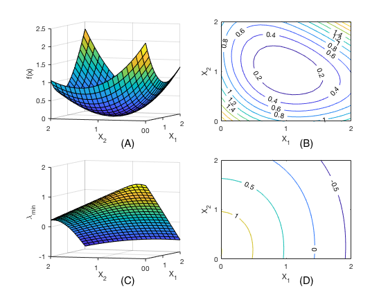
Refer to caption
Figure 1: Simulation results for the Lyapunov Function PDE (47): (a) f⁡(x)f(x); (b) the contours of f⁡(x)f(x); (c) λmin\lambda_{\mathrm{min}}; (d) the contours of λm​i​n\lambda_{min}.

7 Conclusion and a Conjecture

This paper is devoted to developing the Lyapunov function with clear physical meaning for stability analysis for chemical reaction networks. We have attempted to address this issue by establishing approximation from a microscopic concept of CRNs, the scaling non-equilibrium potential, to the macroscopic notation of the candidate Lyapunov function. After rewriting the Chemical Master Equation skillfully, we have succeeded in implementing the approximation and transformed the ODE into a PDE, which together with the developed boundary condition yields the Lyapunov Function PDEs. And then, we have proved that the solution (if exists) of the PDEs is dissipative, and thus has great potential to become a Lyapunov function. Next, we have applied the Lyapunov Function PDEs to complex-balanced CRNs and general CRNs with 11-dimensional stoichiometric subspace. For both cases, we construct their solutions that can act as Lyapunov functions rendering the respective system to be locally asymptotically stable. Finally, we have extended the applications of the Lyapunov Function PDEs to some special CRNs with more than 22-dimensional stoichiometric subspace, and showed that the PDEs also work validly for them in stability analysis.

Notwithstanding the performance illustrated by the Lyapunov Function PDEs is very encouraging, there are still some problems needed to be explored in the future. One of the most urgent problems is to prove that the Lyapunov Function PDEs CAN or CANNOT serve for general CRNs with more than 22-dimensional stoichiometric subspace. This may be an extremely arduous task, however, we are inclined to think they can. We summarize the proof task as a conjecture: “For any mass action system that admits a stable positive equilibrium, if the boundary complex set is equipped properly, then the Lyapunov Function PDEs induced by this system have a solution qualified as a Lyapunov function to suggest the system to be locally asymptotically stable at the equilibrium.” The converse problem is also interesting, i.e., will all Lyapunov functions be solutions to the PDEs in some sense?

References

  • [1] M. Ali Al-Radhawi and D. Angeli, New approach to the stability of chemical reaction networks: Piecewise linear in rates lyapunov functions, IEEE T. Automat. Contr., 61 (2016), pp. 76–89.
  • [2] D. F. Anderson, G. Craciun, M. Gopalkrishnan, and C. Wiuf, Lyapunov functions, stationary distributions, and non-equilibrium potential for reaction networks, B. Math. Biol., 77 (2015), pp. 1744–1767.
  • [3] D. F. Anderson, G. Craciun, and T. G. Kurtz, Product-form stationary distributions for deficiency zero chemical reaction networks, B. Math. Biol., 72 (2010), pp. 1947–1970.
  • [4] D. F. Anderson and T. G. Kurtz, Continuous time markov chain models for chemical reaction networks, in Design and analysis of biomolecular circuits, Springer, 2011, pp. 3–42.
  • [5] D. F. Anderson and T. G. Kurtz, Stochastic analysis of biochemical systems, vol. 1, Springer, 2015.
  • [6] D. Angeli, A tutorial on chemical reaction network dynamics, Eur. J. Control, 15 (2009), pp. 398–406.
  • [7] D. Angeli, P. De Leenheer, and E. D. Sontag, A petri net approach to the study of persistence in chemical reaction networks, Math. Biosci., 210 (2007), pp. 598–618.
  • [8] G. Craciun, F. Nazarov, and C. Pantea, Persistence and permanence of mass-action and power-law dynamical systems, SIAM Journal on Applied Mathematics, 73 (2013), pp. 305–329.
  • [9] S. N. Ethier and T. G. Kurtz, Markov processes: characterization and convergence, vol. 282, John Wiley & Sons, 2009.
  • [10] M. Feinberg, Complex balancing in general kinetic systems, Arch. Ration. Mech. An., 49 (1972), pp. 187–194.
  • [11] M. Feinberg, Chemical reaction network structure and the stability of complex isothermal reactors??i. the deficiency zero and deficiency one theorems, Chem. Eng. Sci., 42 (1987), pp. 2229–2268.
  • [12] M. Feinberg, Chemical reaction network structure and the stability of complex isothermal reactors??ii. multiple steady states for networks of deficiency one, Chem. Eng. Sci., 43 (1988), pp. 1–25.
  • [13] M. Feinberg, Necessary and sufficient conditions for detailed balancing in mass action systems of arbitrary complexity, Chem. Eng. Sci., 44 (1989), pp. 1819–1827.
  • [14] M. Feinberg, The existence and uniqueness of steady states for a class of chemical reaction networks, Arch. Ration. Mech. An., 132 (1995), pp. 311–370.
  • [15] M. Gopalkrishnan, E. Miller, and A. Shiu, A geometric approach to the global attractor conjecture, SIAM Journal on Applied Dynamical Systems, 13 (2014), pp. 758–797.
  • [16] A. N. Gorban, General h-theorem and entropies that violate the second law, Entropy, 16 (2014), pp. 2408–2432.
  • [17] D. J. Higham, Modeling and simulating chemical reactions, SIAM Rev., 50 (2008), pp. 347–368.
  • [18] F. Horn and R. Jackson, General mass action kinetics, Arch. Ration. Mech. An., 47 (1972), pp. 81–116.
  • [19] T. G. Kurtz, The relationship between stochastic and deterministic models for chemical reactions, The Journal of Chemical Physics, 57 (1972), pp. 2976–2978.
  • [20] Y. Li and Y. Yi, Systematic measures of biological networks ii: Degeneracy, complexity, and robustness, Commun. Pur. Appl. Math., 69 (2016), pp. 1952–1983.
  • [21] Y. Li and Y. Yi, Systematic measures of biological networks, part i: Invariant measures and entropy, Commun. Pur. Appl. Math., 69 (2016), pp. 1777–1811.
  • [22] B. K. Øksendal and A. Sulem, Applied stochastic control of jump diffusions, vol. 498, Springer, 2005.
  • [23] C. Pantea, On the persistence and global stability of mass-action systems, SIAM Journal on Mathematical Analysis, 44 (2012), pp. 1636–1673.
  • [24] S. Rao, A. van der Schaft, and B. Jayawardhana, A graph-theoretical approach for the analysis and model reduction of complex-balanced chemical reaction networks, J. Math. Chem., 51 (2013), pp. 2401–2422.
  • [25] S. I. Resnick, Adventures in stochastic processes, Springer Science & Business Media, 2013.
  • [26] D. Siegel and D. MacLean, Global stability of complex balanced mechanisms, Journal of Mathematical Chemistry, 27 (2000), pp. 89–110.
  • [27] E. D. Sontag, Structure and stability of certain chemical networks and applications to the kinetic proofreading model of t-cell receptor signal transduction, IEEE T. Automat. Contr., 46 (2001), pp. 1028–1047.
  • [28] G. Szederkényi and K. M. Hangos, Finding complex balanced and detailed balanced realizations of chemical reaction networks, J. Math. Chem., 49 (2011), pp. 1163–1179.
  • [29] A. van der Schaft, S. Rao, and B. Jayawardhana, On the mathematical structure of balanced chemical reaction networks governed by mass action kinetics, SIAM J. Appl. Math., 73 (2013), pp. 953–973.