跳到论文正文
W Papers独立论文阅读器 arXiv:1510.03483 论文正文 计算阅读时间 · 0%
引用这篇论文根据当前论文元数据生成,正式投稿前建议核对。


License: arXiv.org perpetual non-exclusive license
arXiv:1510.03483v2 [math.GT] 05 Apr 2019

Quantum 𝔤​𝔩1|1\mathfrak{gl}_{1|1} and tangle Floer homology

Alexander P. Ellis Email address: apellis@gmail.com URL: http://ape.wtf , Ina Petkova Address: Department of Mathematics, Dartmouth College
Hanover, NH 03755
Email address: ina.petkova@dartmouth.edu URL: http://math.dartmouth.edu/˜ina
and Vera Vértesi Address: Institut de Recherche Mathématique Avancée
Université de Strasbourg
Email address: vertesi@math.unistra.fr
Abstract.

We identify the Grothendieck group of the tangle Floer dg algebra with a tensor product of certain Uq​(𝔤​𝔩1|1)U_{q}(\mathfrak{gl}_{1|1}) representations. Under this identification, up to a scalar factor, the map on the Grothendieck group induced by the tangle Floer dg bimodule associated to a tangle agrees with the Reshetikhin-Turaev homomorphism for that tangle. We also introduce dg bimodules which act on the Grothendieck group as the generators EE and FF of Uq​(𝔤​𝔩1|1)U_{q}(\mathfrak{gl}_{1|1}).

Key words and phrases: 
tangles, knot Floer homology, quantum groups, TQFT
2010 Mathematics Subject Classification
57M27; 20G42

1. Introduction

1.1. Alexander and Jones

The Reshetikhin-Turaev construction [RT91] is a machine for turning a representation WW of a quantized enveloping algebra Uq​(𝔤)U_{q}(\mathfrak{g}) into a tangle invariant. It takes:

  1. (1)

    a sequence of oriented points to a tensor product of copies of WW and W∗W^{*} and

  2. (2)

    a tangle 𝒯\mathcal{T} to a Uq​(𝔤)U_{q}(\mathfrak{g}) intertwiner RT⁡(𝒯){\rm{RT}}(\mathcal{T}) between the representations associated to its incoming and outgoing boundaries.

The map associated to a tangle is an invariant of the tangle.

Special cases include the Jones polynomial (𝔤=𝔰​𝔩2\mathfrak{g}=\mathfrak{sl}_{2}, WW the vector representation UU) and the Alexander polynomial (𝔤=𝔤​𝔩1|1\mathfrak{g}=\mathfrak{gl}_{1|1}, WW the vector representation VV). As interesting as these invariants are, more interesting still are their lifts—categorifications—to more complicated invariants.

Khovanov homology is the poster child for categorification. In its formulation for tangles [CK14, BS11], it takes:

  1. (1)

    a sequence of nn points to a graded ring HnH_{n} and

  2. (2)

    an (m,n)(m,n)-tangle 𝒯\mathcal{T} to a complex C𝐾ℎ​(𝒯)C_{\mathit{Kh}}(\mathcal{T}) of bimodules over (Hm,Hn)(H_{m},H_{n}).

(See also the earlier work in [Kho02] and the more geometrically flavored [BN05] when mm and nn are even.) The homotopy equivalence class of C𝐾ℎ​(𝒯)C_{\mathit{Kh}}(\mathcal{T}) is an invariant of the tangle. Identifying a basis for the (complexified) Grothendieck group of the category of such complexes with a basis for HomUq​(𝔰​𝔩2)⁡(U⊗m,U⊗n)\Hom_{U_{q}(\mathfrak{sl}_{2})}(U^{\otimes m},U^{\otimes n}), the functor given by tensor product with C𝐾ℎ​(𝒯)C_{\mathit{Kh}}(\mathcal{T}) acts by RT⁡(𝒯){\rm{RT}}(\mathcal{T}).

Furthermore, Khovanov homology is functorial: with some adjustments, one can associate a homotopy class of homomorphisms of complexes of bimodules over (Hm,Hn)(H_{m},H_{n}) that is an invariant of tangle cobordisms [Kho06, Jac04, MSK09]. The total package, then, is an extended 2D TQFT which categorifies the Reshetikhin-Turaev 1D TQFT.

A more recent approach, initiated by Khovanov-Lauda [KL09, KL10] and Rouquier [Rou08],

seeks to categorify an even wider swath of quantum algebra: quantized enveloping algebras themselves, tensor products of their integrable highest weight representations, the Reshetikhin-Turaev intertwiners, and more. Webster has used this approach to construct link homology theories which categorify the Reshetikhin-Turaev invariant for all representations and Kac-Moody types [Web13] (without the maps for cobordisms).

None of these constructions, however, extend to the case of the Alexander polynomial. There has been some work on the categorification of Uq​(𝔤​𝔩1|1)U_{q}(\mathfrak{gl}_{1|1}) [Kho14, Tia16, Tia14] (see also an approach via u−1​(𝔰​𝔩2)u_{\sqrt{-1}}(\mathfrak{sl}_{2}) [Vir06, EQ16]), but so far, the only categorification of the Alexander polynomial has a rather different, non-representation theoretic origin.

Knot Floer homology, introduced by Ozsváth-Szabó [OS04] and Rasmussen [Ras03], associates a bigraded chain complex CFK^​(ℋ){\rm{\widehat{CFK}}}(\mathcal{H}) to a Heegaard diagram ℋ\mathcal{H} for a link LL. The differential on CFK^​(ℋ){\rm{\widehat{CFK}}}(\mathcal{H}) counts pseudoholomorphic curves with prescribed boundary conditions in an almost complex manifold defined in terms of ℋ\mathcal{H}. The homology of CFK^​(ℋ){\rm{\widehat{CFK}}}(\mathcal{H}) is an invariant of LL denoted HFK^​(L){\rm{\widehat{HFK}}}(L).

Like its distant cousin Khovanov homology, HFK^​(L){\rm{\widehat{HFK}}}(L) has proven to be a powerful invariant. Unfortunately, despite a completely combinatorial description of CFK^​(ℋ){\rm{\widehat{CFK}}}(\mathcal{H}) [MOS09], the invariant is still global in nature; local modifications are only partly understood [OS04, OS09, Man07]. In order to fit HFK^​(L){\rm{\widehat{HFK}}}(L) into the general pattern of Reshetikhin-Turaev invariants, then, two initial hurdles must be addressed: locality and the relation to Uq​(𝔤​𝔩1|1)U_{q}(\mathfrak{gl}_{1|1}).

1.2. Jumping hurdles

In 2014, the second and third authors introduced a local construction of knot Floer homology [PV16a]. A dg algebra A⁡(P)A(P) is associated to each oriented 00-manifold PP, and a dg bimodule CT~​(𝒯)\widetilde{\rm{CT}}(\mathcal{T}) is associated to each oriented tangle 𝒯\mathcal{T}. For a closed tangle, i.e. a link, this bimodule agrees with knot Floer homology tensored with a 22-dimensional vector space. The general structure should feel familiar to any bordered Heegaard Floer homologist: the bimodules in question are type 𝐷𝐴\mathit{DA} structures in the sense of [LOT15], composition of these bimodules is via the box tensor product, and while the algebras and bimodules of [PV16a] admit combinatorial descriptions inspired by Heegaard diagrams, the proof of invariance is topological and analytic.

The Alexander polynomial, then, admits a categorification with local pieces very much like its construction as a Reshetikhin-Turaev invariant. The wildly optimistic reader will expect these local pieces to categorify their Reshetikhin-Turaev counterparts.

Fortunately, this optimism is rewarded.

In Subsection 2.3, to a sign sequence P∈{±1}nP\in\{\pm 1\}^{n} we associate the Uq​(𝔤​𝔩1|1)U_{q}(\mathfrak{gl}_{1|1})-representation VP⊗L⁡(λP)V_{P}\otimes L(\lambda_{P}), where VPV_{P} is a tensor product of copies of VV and V∗V^{*} (VV for plus and V∗V^{*} for minus) and L⁡(λP)L(\lambda_{P}) is an appropriately chosen 22-dimensional representation depending on PP, and a basis BB for VP⊗L⁡(λP)V_{P}\otimes L(\lambda_{P}) whose vectors are in bijection with subsets of [n]={0,1,…,n}[n]=\{0,1,\ldots,n\}.

The dg algebra A⁡(P)A(P) has primitive idempotents in bijection with subsets of the set [n][n]. Write e𝐬e_{{\bf s}} for the primitive idempotent corresponding to 𝐬⊆[n]{\bf s}\subseteq[n].

Theorem A.

Let P=(P1,…,Pn)∈{±1}nP=(P_{1},\ldots,P_{n})\in\{\pm 1\}^{n} be a sign sequence. Then the Grothendieck group of dg modules over the dg algebra A⁡(P)A(P) is a free ℤ⁡[q±1]\mathbb{Z}[q^{\pm 1}]-module with basis {[A⁡(P)​e𝐬]∣𝐬⊆[n]}\{[A(P)e_{{\bf s}}]\mid{\bf s}\subseteq[n]\}. Identifying the basis vector [A⁡(P)​e𝐬][A(P)e_{{\bf s}}] with the basis vector in BB associated to the subset 𝐬{\bf s} determines an isomorphism of vector spaces

K0​(A⁡(P))⊗ℤ⁡[q±1]ℂ⁡(q)≅VP⊗L⁡(λP).K_{0}(A(P))\otimes_{\mathbb{Z}[q^{\pm 1}]}\mathbb{C}(q)\cong V_{P}\otimes L(\lambda_{P}).

Let 𝒯\mathcal{T} be a tangle and color each strand of 𝒯\mathcal{T} by the vector representation VV. Under the identification above, up to an overall factor of a positive integer power of (1−q−2)(1-q^{-2}) , box tensor product with the type 𝐷𝐴\mathit{DA} bimodule CT~​(𝒯)\widetilde{\rm{CT}}(\mathcal{T}) acts on K0​(A​(P))K_{0}(A(P)) as the Reshetikhin-Turaev intertwiner associated to the colored tangle 𝒯\mathcal{T} tensored with idL⁡(λP)\id_{L(\lambda_{P})} (see Figure 1). The precise statement is given in Equation (50). 11 1 The appearance of the extra representation L⁡(λP)L(\lambda_{P}) is possibly related to the fact that tangle Floer homology recovers knot Floer homology tensored with a 22-dimensional vector space, rather than knot Floer homology alone.

\labellist\pinlabel

𝒯\mathcal{T} at 128 90 \pinlabel 𝒯\mathcal{T} at 360 80 \pinlabelK0(A(−∂0𝒯))←[CT~]K0(A(∂1𝒯))K_{0}(A(-\partial^{0}\mathcal{T}))\xleftarrow{[\widetilde{\rm{CT}}]}K_{0}(A(\partial^{1}\mathcal{T})) at 126 25 \pinlabel== at 282 80 \pinlabelV∂1𝒯V_{\partial^{1}\mathcal{T}} at 432 30 \pinlabel↑\Big\uparrow at 432 80 \pinlabelV−∂0𝒯V_{-\partial^{0}\mathcal{T}} at 432 130 \pinlabelRT{\rm{RT}} at 418 80 \pinlabel⊗\otimes at 484 80 \pinlabelL⁡(λ∂1𝒯)L(\lambda_{\partial^{1}\mathcal{T}}) at 544 30 \pinlabel↑\Big\uparrow at 544 80 \pinlabelL⁡(λ∂1𝒯)L(\lambda_{\partial^{1}\mathcal{T}}) at 544 130 \pinlabelid\id at 556 80 \endlabellistRefer to caption

Figure 1. The Reshetikhin-Turaev invariant RT⁡(𝒯){\rm{RT}}(\mathcal{T}) for the Uq​(𝔤​𝔩1|1)U_{q}(\mathfrak{gl}_{1|1})-representation VV, later denoted by Q⁡(𝒯)Q(\mathcal{T}), corresponds to the action of CT~​(𝒯)\widetilde{\rm{CT}}(\mathcal{T}) on K0​(A​(P))K_{0}(A(P)).

Theorem A is proved in Subsections 4.1 and 4.2.

We also introduce dg bimodules E⁡(P)E(P) and F⁡(P)F(P) over (A⁡(P),A⁡(P))(A(P),A(P)) which act on K0​(A​(P))K_{0}(A(P)) as the elements EE and FF of Uq​(𝔤​𝔩1|1)U_{q}(\mathfrak{gl}_{1|1}). In disanalogy with other categorifications of quantized enveloping algebras, these dg bimodules do not arise from induction and restriction with respect to a tower of algebras comprising the dg algebras A⁡(P)A(P).

Theorem B.

For any sign sequence PP, under the identification of the elementary basis with the basis BB from the previous theorem, the actions of the dg bimodules E⁡(P)E(P) and F⁡(P)F(P) on K0​(A​(P))K_{0}(A(P)) equal the actions of E,F∈Uq​(𝔤​𝔩1|1)E,F\in U_{q}(\mathfrak{gl}_{1|1}) on VP⊗L⁡(λP)V_{P}\otimes L(\lambda_{P}).

There are quasi-isomorphisms

E(P)⊗~A⁡(P)E(P)≃0,F(P)⊗~A⁡(P)F(P)≃0.E(P)\mathbin{\widetilde{\otimes}}_{A(P)}E(P)\simeq 0,\quad F(P)\mathbin{\widetilde{\otimes}}_{A(P)}F(P)\simeq 0.

Furthermore, there is a distinguished triangle

E(P)⊗~A⁡(P)F(P)\textstyle{E(P)\mathbin{\widetilde{\otimes}}_{A(P)}F(P)\ignorespaces\ignorespaces\ignorespaces\ignorespaces}A⁡(P)\textstyle{A(P)\ignorespaces\ignorespaces\ignorespaces\ignorespaces}F(P)⊗~A⁡(P)E(P)\textstyle{F(P)\mathbin{\widetilde{\otimes}}_{A(P)}E(P)\ignorespaces\ignorespaces\ignorespaces\ignorespaces}E(P)⊗~A⁡(P)F(P)[1],\textstyle{E(P)\mathbin{\widetilde{\otimes}}_{A(P)}F(P)[1],}

in 𝒟⁡(A⁡(P))\mathcal{D}(A(P)). For any tangle 𝒯\mathcal{T},

E(−∂0𝒯)⊠CT~(𝒯)≃A(−∂0𝒯)⊠CT~(𝒯)⊗~A⁡(∂1𝒯)E(∂1𝒯),F(−∂0𝒯)⊠CT~(𝒯)≃A(−∂0𝒯)⊠CT~(𝒯)⊗~A⁡(∂1𝒯)F(∂1𝒯)\begin{split}&E(-\partial^{0}\mathcal{T})\boxtimes\widetilde{\rm{CT}}(\mathcal{T})\simeq A(-\partial^{0}\mathcal{T})\boxtimes\widetilde{\rm{CT}}(\mathcal{T})\mathbin{\widetilde{\otimes}}_{A(\partial^{1}\mathcal{T})}E(\partial^{1}\mathcal{T}),\\ &F(-\partial^{0}\mathcal{T})\boxtimes\widetilde{\rm{CT}}(\mathcal{T})\simeq A(-\partial^{0}\mathcal{T})\boxtimes\widetilde{\rm{CT}}(\mathcal{T})\mathbin{\widetilde{\otimes}}_{A(\partial^{1}\mathcal{T})}F(\partial^{1}\mathcal{T})\end{split}

as type 𝐴𝐴\mathit{AA} bimodules over (A(−∂0𝒯),A(∂1𝒯))(A(-\partial^{0}\mathcal{T}),A(\partial^{1}\mathcal{T})).

Theorem B is proved in Subsection 4.3.

1.3. Outline

The reader already conversant with A∞A_{\infty} algebra in the context of bordered Heegaard Floer homology is encouraged to skip Subsections 2.1 and 2.2, which review dg and A∞A_{\infty} algebras, including derived categories of type A\mathit{A} and type D\mathit{D} structures.

In Subsection 2.3, we review the decategorified setting: Uq​(𝔤​𝔩1|1)U_{q}(\mathfrak{gl}_{1|1}), the particular representations we will be concerned with, a canonical basis for these representations, and the Reshetikhin-Turaev maps on these representations. This subsection concludes with a description of how to construct the Alexander polynomial in this language.

Section 3 is an exposition of the tangle Floer package in the language of strand diagrams (see also [PV16a, Section 3]). Since we only need a special case of the general construction, we are able to make several simplifications; see the dictionary in Subsection 3.6. Subsections 3.1 through 3.4 review the construction, and Subsection 3.5 recalls the main theorems of [PV16a].

Theorems A and B are proved in the aptly named Section 4. Subsection 4.1 computes the Grothendieck group of A⁡(P)A(P). Subsection 4.2 computes the action of CT~​(𝒯)\widetilde{\rm{CT}}(\mathcal{T}) on this group and relates the result to the representations VP⊗L⁡(λP)V_{P}\otimes L(\lambda_{P}) and the Reshetikhin-Turaev maps of Subsection 2.3. Subsection 4.3 gives the categorical Uq​(𝔤​𝔩1|1)U_{q}(\mathfrak{gl}_{1|1})-module structure on the derived category of compact dg modules over A⁡(P)A(P).

For the reader uninterested in the details, Section 4 can be understood at a purely formal level after giving Section 3 not much more than a good skim.

Acknowledgments

We thank Mikhail Khovanov, Anthony Licata, Robert Lipshitz, Andy Manion, You Qi, and Joshua Sussan for many helpful comments and conversations. We thank the referees for many useful suggestions. A.P.E. and I.P. each received support from an AMS-Simons travel grant. V.V. was supported by ERC Geodycon, OTKA grant number NK81203 and NSF grant number 1104690.

2. Preliminaries

2.1. A∞A_{\infty} algebras and modules

In this and the following subsection, we review some definitions and constructions from [LOT18, LOT15]. This subsection will review modules and bimodules over dg and A∞A_{\infty} algebras; the next will discuss categories of modules and their Grothendieck groups. For more details, see [LOT15, Section 2]. Throughout, we work over a ground ring 𝐤{\bf k} that is assumed to be a direct sum of a finite number of copies of the two-element field 𝔽2\mathbb{F}_{2}. Although the A∞A_{\infty} algebras in our main construction are all dg algebras, the general A∞A_{\infty} context is more natural, so we will work in that generality. Our review will be brief and mostly serves to establish notation; see [Kel06, LOT15] for more details.

Throughout, we will need to distinguish between homological (later, “Maslov”) and inner (later, “(twice) Alexander”) gradings. The former is the grading which interacts with differentials, A∞A_{\infty} structure maps, and so forth. Structure maps will preserve inner gradings. For a bigraded chain complex VV, we write V⁡[k]V[k] for the complex obtained from VV by decreasing the homological grading by kk. It has graded pieces V​[k]i=Vk+iV[k]_{i}=V_{k+i}. To shift inner rather than homological gradings, we write V​{k}V\{k\}.

Throughout, all algebras and modules will be assumed to be finitely generated.

Write T∗​(V)=⨁k=0∞V⊗kT^{*}(V)=\bigoplus_{k=0}^{\infty}V^{\otimes k} for the tensor algebra of VV and T¯∗​(V)=∏k=0∞V⊗k\overline{T}^{*}(V)=\prod_{k=0}^{\infty}V^{\otimes k} for its completion. The kk-th graded piece of T∗​(V​[1])T^{*}(V[1]) is V⊗k​[k]V^{\otimes k}[k].

Definition 2.1.1.

An A∞A_{\infty} algebra over 𝐤{\bf k} is a (homologically) ℤ\mathbb{Z}-graded 𝐤{\bf k}-bimodule AA equipped with degree 00 𝐤{\bf k}-linear maps

μi:A⊗i→A⁡[2−i]​ for ​i=1,2,…\mu_{i}:A^{\otimes i}\to A[2-i]\text{ for }i=1,2,\ldots

satisfying a certain compatibility condition. To state this condition, we first define a degree 11 𝐤{\bf k}-linear map DA:T∗​(A⁡[1])→T∗​(A⁡[1])D^{A}:T^{*}(A[1])\to T^{*}(A[1]). On (A⁡[1])⊗n(A[1])^{\otimes n}, DAD^{A} acts as

DA|(A⁡[1])⊗n=∑j=1n∑ℓ=1n−j+1idA⊗(j−1)⊗μℓ⊗idA⊗(n−ℓ−j+1).D^{A}|_{(A[1])^{\otimes n}}=\sum_{j=1}^{n}\sum_{\ell=1}^{n-j+1}\id_{A}^{\otimes(j-1)}\otimes\mu_{\ell}\otimes\id_{A}^{\otimes(n-\ell-j+1)}. (1)

The compatibility condition is that

DA∘DA=0D^{A}\circ D^{A}=0 (2)

(or, equivalently, that the part of DA∘DAD^{A}\circ D^{A} with image in A⁡[1]A[1] is zero).

Intuitively, the condition says that the sum over all ways to apply two of the μi\mu_{i}’s in sequence is zero. There is also a graphical formulation in terms of trees (see, for instance, [LOT15]).

Definition 2.1.2.

We say an A∞A_{\infty} algebra AA is (strictly) unital if there is an element 1∈A1\in A such that μ2​(1,a)=μ2​(a,1)=a\mu_{2}(1,a)=\mu_{2}(a,1)=a for all a∈Aa\in A and μk​(a1,…,ak)=0\mu_{k}(a_{1},\ldots,a_{k})=0 if k>2k>2 and aj=1a_{j}=1 for some jj. A strictly unital A∞A_{\infty} algebra AA is augmented if it is equipped with a 𝐤{\bf k}-linear map ϵ:A→𝐤\epsilon:A\to{\bf k} such that ϵ⁡(1)=1\epsilon(1)=1, ϵ⁡(μ2​(a1,a2))=ϵ⁡(a1)​ϵ​(a2)\epsilon(\mu_{2}(a_{1},a_{2}))=\epsilon(a_{1})\epsilon(a_{2}), and ϵ∘μk=0\epsilon\circ\mu_{k}=0 for k≠2k\neq 2. If AA is unital and augmented, we write A+A_{+} for ker⁡(ϵ)\ker(\epsilon).

From now on, we assume all A∞A_{\infty} algebras to be strictly unital and augmented. Let AA be an A∞A_{\infty} algebra over 𝐤{\bf k}. Undecorated tensor products are assumed to be taken over 𝐤{\bf k}.

Definition 2.1.3.

A right A∞A_{\infty} module over AA (also called a right type A\mathit{A} structure over AA) is a graded 𝐤{\bf k}-module MM equipped with degree 11 𝐤{\bf k}-linear maps

mi+1:M⊗(A⁡[1])⊗i→M​ for ​i=0,1,2,…,m_{i+1}:M\otimes(A[1])^{\otimes i}\to M\text{ for }i=0,1,2,\ldots, (3)

satisfying a certain compatibility condition. Assemble all the mim_{i}’s to form a single degree 11 map m:M⊗T∗​(A⁡[1])→Mm:M\otimes T^{*}(A[1])\to M, as we did for DAD^{A} above. Then the compatibility condition is that

m1∘m+m∘(idM⊗DA)=0.m_{1}\circ m+m\circ(\id_{M}\otimes D^{A})=0. (4)

A type A\mathit{A} structure is strictly unital if m2​(x,1)=xm_{2}(x,1)=x and mi​(x,a1,⋯,ai−1)=0m_{i}(x,a_{1},\cdots,a_{i-1})=0 if i>2i>2 and some aj∈𝐤a_{j}\in{\bf k}. If MM is strictly unital, then equivalently, we can restrict mm to M⊗T∗​(A+​[1])M\otimes T^{*}(A_{+}[1]) and impose the same condition (4) on this restriction.

In the case that AA is a dg algebra (meaning μi=0\mu_{i}=0 for i>2i>2) with differential dA=μ1d_{A}=\mu_{1}, the type A\mathit{A} module condition simplifies to

0=∑i+j=n+1mi​(mj​(x,a1,⋯,aj−1),⋯,an−1)+∑i=1n−1mn(x,a1,⋯,ai−1,dA(ai),⋯,an−1)+∑i=1n−2mn−1(x,a1,⋯,ai−1,aiai+1,⋯,an−1)\begin{split}0&=\sum_{i+j=n+1}m_{i}(m_{j}(x,a_{1},\cdots,a_{j-1}),\cdots,a_{n-1})\\ &\qquad+\sum_{i=1}^{n-1}m_{n}(x,a_{1},\cdots,a_{i-1},d_{A}(a_{i}),\cdots,a_{n-1})\\ &\qquad+\sum_{i=1}^{n-2}m_{n-1}(x,a_{1},\cdots,a_{i-1},a_{i}a_{i+1},\cdots,a_{n-1})\end{split}

for all n≥1n\geq 1. If we further assume that MM is a dg module (meaning mi=0m_{i}=0 for i>2i>2) with differential dM=m1d_{M}=m_{1}, the condition simplifies to

n=1:dM2=0,n=2:m2(dM(x),a)+dM(m2(x,a))+m2(x,dA(a))=0,n=3:m2(m2(x,a),b)+m2(x,ab)=0.\begin{split}&n=1:\qquad d_{M}^{2}=0,\\ &n=2:\qquad m_{2}(d_{M}(x),a)+d_{M}(m_{2}(x,a))+m_{2}(x,d_{A}(a))=0,\\ &n=3:\qquad m_{2}(m_{2}(x,a),b)+m_{2}(x,ab)=0.\end{split}

We assume all type A\mathit{A} structures to be strictly unital. Left type A\mathit{A} structures can be defined analogously. We will write MA\prescript{}{A}{M} (respectively MAM_{A}) to indicate that MM is a left (respectively right) module over AA.

We say that MM is bounded if mi=0m_{i}=0 for all sufficiently large ii.

Definition 2.1.4.

A left type D\mathit{D} structure over AA is a graded 𝐤{\bf k}-module NN equipped with a degree 00 𝐤{\bf k}-linear homogeneous map

δ1:N→(A⊗N)​[1]\delta^{1}:N\to(A\otimes N)[1]

satisfying a certain compatibility condition. To state this condition, define maps

δk:N→(A⁡[1])⊗k⊗N\delta^{k}:N\to(A[1])^{\otimes k}\otimes N

for k≥0k\geq 0 inductively by δ0=idN\delta^{0}=\id_{N} and

δk=(idA⊗(k−1)⊗δ1)∘δk−1​ for ​k≥2.\delta^{k}=(\id_{A^{\otimes(k-1)}}\otimes\delta^{1})\circ\delta^{k-1}\text{ for }k\geq 2. (5)

Define a map δ:N→T¯∗​(A⁡[1])\delta:N\to\overline{T}^{*}(A[1]) by

δ⁡(x)=∑i=0∞δi​(x).\delta(x)=\sum_{i=0}^{\infty}\delta^{i}(x).

The compatibility condition is then

(μ⊗idN)∘δ⁡(x)=0.(\mu\otimes\id_{N})\circ\delta(x)=0. (6)

Right type D\mathit{D} structures can be defined analogously. We write NA\prescript{A}{}{N} (respectively NAN^{A}) to indicate that NN is a left (respectively right) type D\mathit{D} structure over AA.

A type D\mathit{D} structure is bounded if for any x∈Nx\in N, δi​(x)=0\delta^{i}(x)=0 for all sufficiently large ii.

If MAM_{A} is a right A∞A_{\infty} module over AA and NA\prescript{A}{}{N} is a left type D\mathit{D} structure over AA, and at least one of them is bounded, we can define the box tensor product M⊠N=MA⊠NAM\boxtimes N=M_{A}\boxtimes\prescript{A}{}{N} to be the vector space M⊗𝐤NM\otimes_{\bf k}N with differential

∂:M⊗N→(M⊗N)​[1]\partial:M\otimes N\to(M\otimes N)[1]

defined by

∂=∑k=1∞(mk⊗idN)∘(idM⊗δk−1).\partial=\sum_{k=1}^{\infty}(m_{k}\otimes\id_{N})\circ(\id_{M}\otimes\delta^{k-1}).

The boundedness condition guarantees that the above sum is finite. In that case ∂2=0\partial^{2}=0, and M⊠NM\boxtimes N is a graded chain complex. The box tensor product is a model for the derived tensor product of two type A\mathit{A} modules, as we explain in the following subsection. The idea: AAA⊠NA\prescript{}{A}{A}_{A}\boxtimes\prescript{A}{}{N} is a left type A\mathit{A} module, and M⊠NM\boxtimes N is homotopy equivalent to the usual derived tensor product (which we define below) M⊗~A(A⊠N)M\mathbin{\widetilde{\otimes}}_{A}(A\boxtimes N). The advantage to M⊠NM\boxtimes N is that it is often finite dimensional, while M⊗~A(A⊠N)M\mathbin{\widetilde{\otimes}}_{A}(A\boxtimes N) is always infinite dimensional.

Given dg algebras AA and BB over 𝐤{\bf k} and 𝐣{\bf j} with differentials and multiplications dAd_{A}, dBd_{B}, μA\mu_{A}, and μB\mu_{B}, respectively, four types of bimodules can be defined in a similar way: types 𝐷𝐷\mathit{DD}, 𝐴𝐴\mathit{AA}, 𝐷𝐴\mathit{DA}, and 𝐴𝐷\mathit{AD}. See [LOT15, Section 2.2.4] for details; we will review them briefly.

An A∞A_{\infty} bimodule or type 𝐴𝐴\mathit{AA} bimodule over (A,B)(A,B) is a graded (𝐤,𝐣)({\bf k},{\bf j})-bimodule MM, together with degree 00 maps

mi,1,j:(A⁡[1])⊗i⊗M⊗(B⁡[1])⊗j→Mm_{i,1,j}:(A[1])^{\otimes i}\otimes M\otimes(B[1])^{\otimes j}\to M

subject to compatibility conditions analogous to those for type AA structures, see [LOT15, Equation 2.2.38].

We assume all type 𝐴𝐴\mathit{AA} bimodules to be strictly unital: m1,1,0​(1,x)=x=m0,1,1​(x,1)m_{1,1,0}(1,x)=x=m_{0,1,1}(x,1) and mi,1,j​(a1,…,ai,x,b1,…,bj)=0m_{i,1,j}(a_{1},\ldots,a_{i},x,b_{1},\ldots,b_{j})=0 if i+j>1i+j>1 and some aia_{i} or bjb_{j} lies in 𝐤{\bf k} or 𝐣{\bf j}.

A type 𝐷𝐴\mathit{DA} bimodule over (A,B)(A,B) is a graded (𝐤,𝐣)({\bf k},{\bf j})-bimodule MM, together with degree 00, (𝐤,𝐣)({\bf k},{\bf j})-linear maps

δ1+j1:M⊗B​[1]⊗j→A⊗M⁡[1],\delta^{1}_{1+j}:M\otimes B[1]^{\otimes j}\to A\otimes M[1],

satisfying a compatibility condition combining those for type A\mathit{A} and D\mathit{D} structures, see [LOT15, Definition 2.2.42].

A type 𝐴𝐷\mathit{AD} structure can be defined similarly, with the roles of AA and BB interchanged.

A type 𝐷𝐷\mathit{DD} structure over (A,B)(A,B) is a type D\mathit{D} structure over A⊗𝔽2BopA\otimes_{\mathbb{F}_{2}}B^{\mathrm{op}}. In other words, it is a graded (𝐤,𝐣)({\bf k},{\bf j})-bimodule MM and a degree 00 map δ1:M→A⊗M⊗B⁡[1]\delta^{1}:M\to A\otimes M\otimes B[1], again with an appropriate compatibility condition.

When AA is the trivial algebra {1}\{1\}, a type 𝐴𝐷\mathit{AD} structure over (A,B)(A,B) is the same thing as a right type D\mathit{D} structure over BB. Similar statements hold for other bimodule structure types, mut. mut.

There are notions of boundedness for bimodules similar to those for one-sided modules. For each compatible pair of bimodule types, there is a corresponding box tensor product. When forming a box tensor product, we always assume that one of the factors is bounded. We illustrate the idea below for the box tensor product of two type 𝐷𝐴\mathit{DA} structures; for details, see [LOT15, Section 2.3.2].

Let MM be a type 𝐷𝐴\mathit{DA} module over (A,B)(A,B) and NN a type 𝐷𝐴\mathit{DA} bimodule over (B,C)(B,C). As a chain complex, define

MBA⊠NCB=ℱ1​(MBA)⊠ℱ2​(NCB),\prescript{A}{}{M}_{B}\boxtimes\prescript{B}{}{N}_{C}=\mathcal{F}_{1}(\prescript{A}{}{M}_{B})\boxtimes\mathcal{F}_{2}(\prescript{B}{}{N}_{C}), (7)

where ℱ1​(MBA)\mathcal{F}_{1}(\prescript{A}{}{M}_{B}) is the right type A\mathit{A} structure over BB obtained from MBA\prescript{A}{}{M}_{B} by forgetting its left type D\mathit{D} structure over AA (and analogously for ℱ2​(NCB)\mathcal{F}_{2}(\prescript{B}{}{N}_{C})). This chain complex can be given the structure of a type 𝐷𝐴\mathit{DA} bimodule over (A,C)(A,C) in a natural way.

2.2. Categories and Grothendieck groups of A∞A_{\infty} modules

Besides [LOT15, Section 2], helpful references for the material in this section include [BL94, Kel06, Kho14]. We will work in the language of A∞A_{\infty} and dg categories. While we recommend [Kel06] as a reference for these, the reader is invited to not worry about the details and instead let the analogy “A∞A_{\infty} categories over 𝐤{\bf k} are to A∞A_{\infty} algebras over 𝐤{\bf k} as 𝐤{\bf k}-linear categories are to 𝐤{\bf k}-algebras” be their guide. In other words, A∞A_{\infty} categories have higher compositions, and compositions hold up to homotopies of homotopies of…ad. inf.

2.2.1. Categories of type A\mathit{A} modules

Let AA be an A∞A_{\infty} algebra and MA,NAM_{A},N_{A} right type A\mathit{A} modules over AA. Define

MorA​(M,N)=Hom𝐤⁡(M⊗T∗​(A+​[1]),N),\mathrm{Mor}_{A}(M,N)=\Hom_{\bf k}(M\otimes T^{*}(A_{+}[1]),N),

the morphism space of type A\mathit{A} maps from MM to NN. The usual differential

d⁡(f)=dN∘f+f∘dMd(f)=d_{N}\circ f+f\circ d_{M}

makes MorA​(M,N)\mathrm{Mor}_{A}(M,N) into a chain complex. We use these as the morphism spaces to define the A∞A_{\infty} category ModA\mathrm{Mod}_{A} of right type A\mathit{A} modules over AA. The cycles of MorA​(M,N)\mathrm{Mor}_{A}(M,N) are the A∞A_{\infty} homomorphisms from MAM_{A} to NAN_{A}, and the boundaries are called null-homotopic morphisms. Explicitly, a morphism f:M→Nf:M\to N is null-homotopic if there is a degree −1-1 map hh such that

h∘μ1M+μ1N∘h=f.h\circ\mu_{1}^{M}+\mu_{1}^{N}\circ h=f. (8)

Define the dg category ModA\prescript{}{A}{\mathrm{Mod}} of left type A\mathit{A} modules over AA analogously.

When AA is an A∞A_{\infty} algebra, there are two models for the derived category of AA-modules:

  • •

    the 00-th homology category H⁡(ModA)H(\prescript{}{A}{\mathrm{Mod}}) (same objects as ModA\prescript{}{A}{\mathrm{Mod}}, quotient each morphism space by the subspace of null-homotopic morphisms);

  • •

    the localization of ModA\prescript{}{A}{\mathrm{Mod}} at the class of quasi-isomorphisms (morphisms which induce an isomorphism on homology).

These two categories are equivalent as triangulated categories [LOT15, Proposition 2.4.1].

If AA is a dg algebra, then there are three more models for the derived category:

  • •

    dg modules and homotopy classes of dg module homomorphisms, localized at the class of quasi-isomorphisms;

  • •

    dg modules and homotopy classes of A∞A_{\infty} homomorphisms;

  • •

    the localization of the previous at the class of quasi-isomorphisms.

All five models are equivalent as triangulated categories [LOT15, Proposition 2.4.1]. By abuse of notation, write 𝒟⁡(A)\mathcal{D}(A) for any of these triangulated categories.

For the rest of this subsection, we restrict to the case where AA is a dg algebra and use the dg modules, dg homomorphisms model of 𝒟⁡(A)\mathcal{D}(A). In our main construction later, all A∞A_{\infty} algebras will be dg algebras.

In this case, the shift functor 𝒟⁡(A)→𝒟⁡(A)\mathcal{D}(A)\to\mathcal{D}(A) is given on objects by (M,dM)↦(M⁡[1],−dM)(M,d_{M})\mapsto(M[1],-d_{M}). The distinguished triangles are those isomorphic to triangles of the form

M\textstyle{M\ignorespaces\ignorespaces\ignorespaces\ignorespaces}f\scriptstyle{f}N\textstyle{N\ignorespaces\ignorespaces\ignorespaces\ignorespaces}C⁡(f)\textstyle{C(f)\ignorespaces\ignorespaces\ignorespaces\ignorespaces}M⁡[1],\textstyle{M[1],}

where C⁡(f)C(f) is the cone of ff, and the maps in and out of C⁡(f)C(f) are the evident inclusion and projection maps. This triangulated structure can also be obtained by viewing the category of dg modules and dg module homomorphisms as a Frobenius category and identifying 𝒟⁡(A)\mathcal{D}(A) with its stable category [Kel06].

Let ℋ⁡(A)\mathcal{H}(A) be the usual homotopy category of dg modules over AA: objects are left dg modules over AA, and morphisms spaces are the quotient of all dg homomorphisms by the null-homotopic homomorphisms.

In the derived category of an ordinary algebra, morphism spaces can be computed by taking projective resolutions. The analogous notion in dg algebra is that of a cofibrant module (also called “projective” in [Kho14], “K-projective” in [BL94]). We say a dg module PP over AA is cofibrant if whenever we are given a surjective quasi-isomorphism L→ML\to M and a morphism P→MP\to M, we can factor the latter through LL,

P\textstyle{P\ignorespaces\ignorespaces\ignorespaces\ignorespaces}L\textstyle{L\ignorespaces\ignorespaces\ignorespaces\ignorespaces\ignorespaces\ignorespaces\ignorespaces\ignorespaces}≃\scriptstyle{\simeq}∃\scriptstyle{\exists}M.\textstyle{M.}

Let ℋ𝑐𝑓​(A)\mathcal{H}_{\mathit{cf}}(A) be the smallest subcategory of ℋ⁡(A)\mathcal{H}(A) containing all cofibrant modules and closed under arbitrary direct sums. Then the restriction of the localization functor ℋ⁡(A)→𝒟⁡(A)\mathcal{H}(A)\to\mathcal{D}(A) to ℋ𝑐𝑓​(A)\mathcal{H}_{\mathit{cf}}(A) is an equivalence of triangulated categories,

ℋ⁡(A)\textstyle{\mathcal{H}(A)\ignorespaces\ignorespaces\ignorespaces\ignorespaces}𝒟⁡(A).\textstyle{\mathcal{D}(A).}ℋ𝑐𝑓​(A)\textstyle{\mathcal{H}_{\mathit{cf}}(A)\ignorespaces\ignorespaces\ignorespaces\ignorespaces\ignorespaces\ignorespaces\ignorespaces\ignorespaces}≃\scriptstyle{\simeq}

There is a standard way to choose a cofibrant replacement for a dg (or A∞A_{\infty}) module MM. There is a type 𝐷𝐷\mathit{DD} bimodule BarA(A)A\prescript{A}{}{\BBar}(A)^{A} (see [LOT15, Definition 2.3.16]) such that

Bar(MA)=MA⊠BarA(A)A⊠AAA\BBar(M_{A})=M_{A}\boxtimes\prescript{A}{}{\BBar}(A)^{A}\boxtimes\prescript{}{A}{A}_{A} (9)

is cofibrant for any MAM_{A}. This bar resolution is functorial in MAM_{A} and comes with a canonical map Bar⁡(MA)→MA\BBar(M_{A})\to M_{A}. There is the obvious definition for left modules as well.

Remark.

We do not need to localize at the class of quasi-isomorphisms when we use the “dg modules and A∞A_{\infty} homomorphisms modulo homotopy” model because the definition of MorA\prescript{}{A}{\mathrm{Mor}} already includes the bar resolution.

We now turn to Grothendieck groups. If 𝒞\mathcal{C} is a triangulated category (assumed to be essentially small) with shift functor X↦X⁡[1]X\mapsto X[1], then its Grothendieck group K0​(𝒞)K_{0}(\mathcal{C}) is the quotient of the free abelian group on the set of symbols

{[X]∣X​ is an isomorphism class of objects of ​𝒞}\{[X]\mid X\text{ is an isomorphism class of objects of }\mathcal{C}\}

by the following two relations:

  1. (1)

    [Y]=[X]+[Z][Y]=[X]+[Z] for every triangle X→Y→Z→X⁡[1]X\to Y\to Z\to X[1] isomorphic to a distinguished triangle;

  2. (2)

    [X⁡[1]]=−[X][X[1]]=-[X] for every object XX.

As with ordinary algebras, we must restrict to a class of suitably small modules in order to get a nontrivial Grothendieck group (recall the “Eilenberg swindle”, A⊕∞⊕A≅A⊕∞A^{\oplus\infty}\oplus A\cong A^{\oplus\infty}). A useful condition is the following: we say a dg module MM over AA is compact (also called “small” in [Kel06]) if the functor Hom𝒟⁡(A)⁡(M,−)\Hom_{\mathcal{D}(A)}(M,-) commutes with arbitrary direct sums. Let 𝒟c​(A)\mathcal{D}_{c}(A) be the smallest full triangulated subcategory of 𝒟⁡(A)\mathcal{D}(A) that contains all compact objects and is closed under isomorphisms; we call this the compact (or perfect) derived category of AA. Define the Grothendieck group of the dg algebra AA to be

K0​(A)=K0​(𝒟c​(A)).K_{0}(A)=K_{0}(\mathcal{D}_{c}(A)). (10)

This is not necessarily the same as the Grothendieck group of the category of finitely generated (non-dg) projective modules over AA.

A dg bimodule MM over (A,B)(A,B) gives rise to a derived tensor functor

M⊗~B(−):𝒟(B)→𝒟⁡(A),N↦M⊗BBar⁡(N).\begin{split}M\mathbin{\widetilde{\otimes}}_{B}(-):\mathcal{D}(B)&\to\mathcal{D}(A),\\ N&\mapsto M\otimes_{B}\BBar(N).\end{split}

There is also a derived hom functor, right adjoint to the derived tensor functor. If M⊗~B(−)M\mathbin{\widetilde{\otimes}}_{B}(-) sends compact objects to compact objects, then there is an induced homomorphism

[M⊗~B−]:K0(B)→K0(A).[M\mathbin{\widetilde{\otimes}}_{B}-]:K_{0}(B)\to K_{0}(A).

2.2.2. Categories of type D\mathit{D} modules; bimodules and functors

If MA\prescript{A}{}{M} and NA\prescript{A}{}{N} are left type D\mathit{D} structures over AA with respective structure maps δM\delta^{M} and δN\delta^{N}, let

MorA​(MA,NA)=Hom𝐤⁡(M,A⊗N).\prescript{A}{}{\mathrm{Mor}}(\prescript{A}{}{M},\prescript{A}{}{N})=\Hom_{\bf k}(M,A\otimes N). (11)

Write h1h^{1} for an element of this morphism space, and for each i≥2i\geq 2, define hi:M→A⊗i⊗Nh^{i}:M\to A^{\otimes i}\otimes N by

hi=∑j=0i−1(idA⊗(j−1)⊗(δN)i−j−1)∘(idA⊗j⊗h1)∘(δM)jh^{i}=\sum_{j=0}^{i-1}(\id_{A^{\otimes(j-1)}}\otimes(\delta^{N})^{i-j-1})\circ(\id_{A^{\otimes j}}\otimes h^{1})\circ(\delta^{M})^{j} (12)

and h:M→T¯∗​(A)⊗Nh:M\to\overline{T}^{*}(A)\otimes N by h=∑i=1∞hih=\sum_{i=1}^{\infty}h^{i}. We give this space a differential ∂\partial defined by

(∂h)1=(μ⊗idN)∘h.(\partial h)^{1}=(\mu\otimes\id_{N})\circ h. (13)

Let Mod𝔲A\prescript{A}{\mathfrak{u}}{\mathrm{Mod}} be the A∞A_{\infty} category of left type D\mathit{D} structures over AA with these morphism complexes (see [LOT15, Lemma 2.2.27] for the definition of the higher composition maps). When AA is a dg algebra, Mod𝔲A\prescript{A}{\mathfrak{u}}{\mathrm{Mod}} will be a dg category.

Cycles in Mor𝔲A\prescript{A}{\mathfrak{u}}{\mathrm{Mor}} are called homomorphisms of type D\mathit{D} structures. Since any morphism between bounded type D\mathit{D} structures is bounded [LOT15, 2.2.30], the subcategory of bounded type D\mathit{D} structures and bounded morphisms in Mod𝔲A\prescript{A}{\mathfrak{u}}{\mathrm{Mod}} is a full A∞A_{\infty} subcategory. Let ModA\prescript{A}{}{\mathrm{Mod}} be the full A∞A_{\infty} subcategory of left type D\mathit{D} structures homotopy equivalent to a bounded type D\mathit{D} structure.

Functors between categories of left type A\mathit{A} or type D\mathit{D} structures can be constructed using bimodules of appropriate types. For example, suppose MBA\prescript{}{A}{M}^{B} is a type 𝐴𝐷\mathit{AD} bimodule over (A,B)(A,B), bounded as a type D\mathit{D} module. The assignment

NB↦MBA⊠NB\prescript{}{B}{N}\mapsto\prescript{}{A}{M}^{B}\boxtimes\prescript{}{B}{N}

induces functors

ModB→ModA\prescript{}{B}{\mathrm{Mod}}\to\prescript{}{A}{\mathrm{Mod}}

and

𝒟⁡(B)→𝒟⁡(A).\mathcal{D}(B)\to\mathcal{D}(A).

If we were to define functors on the derived category using dg bimodules (rather than type AA or D\mathit{D} bimodules), we would have to use the derived tensor product. This requires taking a cofibrant replacement of one of the factors; in practice, cofibrant replacements of finite dimensional modules are often infinite dimensional (functorial ones, always so). As we presently explain, the category of type D\mathit{D} structures can be used as a model of the category of cofibrant dg modules. Box tensor product with a type 𝐷𝐴\mathit{DA} bimodule takes the place of derived tensor product with a dg (or type 𝐴𝐴\mathit{AA}) bimodule. In our main construction, this technique will allow us to compute classes in K0​(A)K_{0}(A) by dimension counting.

Given a left type D\mathit{D} structure NA\prescript{A}{}{N} over a dg algebra AA, the left box tensor product with the dg bimodule AA over (A,A)(A,A) makes AAA⊠NA\prescript{}{A}{A}_{A}\boxtimes\prescript{A}{}{N} a cofibrant left dg module over AA. If the resulting module is compact, then there is a corresponding class in K0​(A)K_{0}(A). In fact, up to quasi-isomorphism, we get all dg modules over AA in this way:

Proposition 2.2.1 ([LOT15], Proposition 2.3.18).

Let AA be a dg algebra and NA\prescript{A}{}{N} a left type D\mathit{D} structure over AA. The A∞A_{\infty} functors

ModA→ModANA↦AAA⊠NA\begin{split}\prescript{A}{}{\mathrm{Mod}}&\to\prescript{}{A}{\mathrm{Mod}}\\ \prescript{A}{}{N}&\mapsto\prescript{}{A}{A}_{A}\boxtimes\prescript{A}{}{N}\end{split}

and

ModA→ModAMA↦ABar(A)A⊠AM\begin{split}\prescript{}{A}{\mathrm{Mod}}&\to\prescript{A}{}{\mathrm{Mod}}\\ \prescript{}{A}{M}&\mapsto\prescript{A}{}{\BBar(A)}^{A}\boxtimes\prescript{}{A}{M}\end{split}

are homotopy inverse via canonical homotopies.

They intertwine the tensor products ⊠\boxtimes and ⊗~\mathbin{\widetilde{\otimes}} in the sense that there is a canonical homotopy equivalence

MA⊠NA≃MA⊗~(AAA⊠NA)M_{A}\boxtimes\prescript{A}{}{N}\simeq M_{A}\mathbin{\widetilde{\otimes}}(\prescript{}{A}{A}_{A}\boxtimes\prescript{A}{}{N})

for any right type A\mathit{A} module MM and left type D\mathit{D} module NN over AA. In particular, the categories ModA\prescript{A}{}{\mathrm{Mod}} and ModA\prescript{}{A}{\mathrm{Mod}} are quasi-equivalent. Hence their derived categories are equivalent, and their Grothendieck groups are isomorphic.

Corresponding statements hold with left and right exchanged.

We will use Proposition 2.2.1 in the proof of Proposition 4.1.1 below.

Remark.

If a dg algebra AA is considered as a dg category AcA_{c} (objects: primitive idempotents e∈Ae\in A; morphism complexes: primitive idempotented pieces e′​A​ee^{\prime}Ae), then (bounded) type D\mathit{D} structures over AA are equivalent to one-sided twisted complexes over AcA_{c}. We have chosen to use the language of type D\mathit{D} structures because it is more standard in the low dimensional topology literature. For more on twisted complexes, see [BK90].

2.3. Quantum 𝔤​𝔩1|1\mathfrak{gl}_{1|1} and bases for tensor powers of VV and V∗V^{*}

Much of the exposition of this subsection follows the development of [Sar15].

2.3.1. Quantum 𝔤​𝔩1|1\mathfrak{gl}_{1|1}

Let

𝔤​𝔩1|1=Endℂ⁡(ℂ1|1)\mathfrak{gl}_{1|1}=\End_{\mathbb{C}}(\mathbb{C}^{1|1}) (14)

be the Lie superalgebra of superlinear endomorphisms of a (1,1)(1,1) dimensional supervector space. Its Cartan subalgebra is the supervector space

𝔥=span⁡(h1,h2)⊂𝔤​𝔩1|1,\mathfrak{h}=\mathrm{span}(h_{1},h_{2})\subset\mathfrak{gl}_{1|1},

where h1h_{1} (respectively h2h_{2}) is projection onto the subspace ℂ1|0\mathbb{C}^{1|0} (respectively ℂ0|1\mathbb{C}^{0|1}). Let ε1,ε2\varepsilon_{1},\varepsilon_{2} be the basis vectors of 𝔥∗\mathfrak{h}^{*} dual to h1,h2h_{1},h_{2} respectively. We have weight and coweight lattices

𝐏=ℤ​ε1⊕ℤ​ε2⊂𝔥∗,𝐏∗=ℤ​h1⊕ℤ​h2⊂𝔥,\mathbf{P}=\mathbb{Z}\varepsilon_{1}\oplus\mathbb{Z}\varepsilon_{2}\subset\mathfrak{h}^{*},\qquad\mathbf{P}^{*}=\mathbb{Z}h_{1}\oplus\mathbb{Z}h_{2}\subset\mathfrak{h},

respectively. The unique positive root is

α=ε1−ε2.\alpha=\varepsilon_{1}-\varepsilon_{2}.

Let ⟨⋅,⋅⟩\langle\cdot,\cdot\rangle denote the canonical pairing between 𝔥\mathfrak{h} and 𝔥∗\mathfrak{h}^{*},

⟨hi,εj⟩=δi,j.\langle h_{i},\varepsilon_{j}\rangle=\delta_{i,j}. (15)

We define a non-degenerate symmetric bilinear form on 𝔥∗\mathfrak{h}^{*} by

(εi,εj)={1if ​i=j=1,−1if ​i=j=2,0if ​i≠j.(\varepsilon_{i},\varepsilon_{j})=\begin{cases}1&\text{if }i=j=1,\\ -1&\text{if }i=j=2,\\ 0&\text{if }i\neq j.\end{cases} (16)

We give a ℤ/2​ℤ\mathbb{Z}/2\mathbb{Z}-grading to the additive group 𝐏\mathbf{P} by

p⁡(ε1)=0,p⁡(ε2)=1,p(\varepsilon_{1})=0,\quad p(\varepsilon_{2})=1,

so that p⁡(n1​ε1+n2​ε2)=n2p(n_{1}\varepsilon_{1}+n_{2}\varepsilon_{2})=n_{2}.

The Hopf superalgebra Uq=Uq​(𝔤​𝔩1|1)U_{q}=U_{q}(\mathfrak{gl}_{1|1}) is defined as follows. The underlying superalgebra is generated over ℂ⁡(q)\mathbb{C}(q) by EE (odd), FF (odd), and {𝐪h:h∈𝐏∗}\{\mathbf{q}^{h}:h\in\mathbf{P}^{*}\} (all even) subject to the relations

𝐪0=1,𝐪h𝐪h′=𝐪h+h′ for all h,h′∈𝐏∗,𝐪hE=q⟨h,α⟩E𝐪h, for all h∈𝐏∗,𝐪h​F=q−⟨h,α⟩​F​𝐪h​ for all ​h∈𝐏∗,E2=F2=0,E​F+F​E=K−K−1q−q−1.\begin{split}&\mathbf{q}^{0}=1,\\ &\mathbf{q}^{h}\mathbf{q}^{h^{\prime}}=\mathbf{q}^{h+h^{\prime}}\text{ for all }h,h^{\prime}\in\mathbf{P}^{*},\\ &\mathbf{q}^{h}E=q^{\langle h,\alpha\rangle}E\mathbf{q}^{h},\text{ for all }h\in\mathbf{P}^{*},\\ &\mathbf{q}^{h}F=q^{-\langle h,\alpha\rangle}F\mathbf{q}^{h}\text{ for all }h\in\mathbf{P}^{*},\\ &E^{2}=F^{2}=0,\\ &EF+FE=\frac{K-K^{-1}}{q-q^{-1}}.\end{split}

We have used the shorthand definition K=𝐪h1+h2K=\mathbf{q}^{h_{1}+h_{2}}. Since ⟨h1+h2,α⟩=0\langle h_{1}+h_{2},\alpha\rangle=0, it follows that K∈Z⁡(Uq​(𝔤​𝔩1|1))K\in Z(U_{q}(\mathfrak{gl}_{1|1})). The coproduct on Uq​(𝔤​𝔩1|1)U_{q}(\mathfrak{gl}_{1|1}) is defined by

Δ⁡(E)=E⊗K−1+1⊗E,Δ⁡(F)=F⊗1+K⊗F,Δ⁡(𝐪h)=𝐪h⊗𝐪h.\begin{split}&\Delta(E)=E\otimes K^{-1}+1\otimes E,\\ &\Delta(F)=F\otimes 1+K\otimes F,\\ &\Delta(\mathbf{q}^{h})=\mathbf{q}^{h}\otimes\mathbf{q}^{h}.\end{split}

The antipode of Uq​(𝔤​𝔩1|1)U_{q}(\mathfrak{gl}_{1|1}) is defined by

S⁡(E)=−E​K,S⁡(F)=−K−1​F,S⁡(𝐪h)=𝐪−h.\begin{split}&S(E)=-EK,\\ &S(F)=-K^{-1}F,\\ &S(\mathbf{q}^{h})=\mathbf{q}^{-h}.\end{split}

Recall that a Hopf superalgebra AA over ℂ⁡(q)\mathbb{C}(q) acts on a tensor product of AA-modules M⊗NM\otimes N by a⋅(m⊗n)=Δ⁡(a)⋅(m⊗n)a\cdot(m\otimes n)=\Delta(a)\cdot(m\otimes n), where A⊗AA\otimes A acts on M⊗NM\otimes N by (a1⊗a2)⋅(m⊗n)=(−1)p⁡(a2)​p​(m)​(a1⋅m)⊗(a2⋅n)(a_{1}\otimes a_{2})\cdot(m\otimes n)=(-1)^{p(a_{2})p(m)}(a_{1}\cdot m)\otimes(a_{2}\cdot n). Also recall that AA acts on the dual M∗=Homℂ⁡(q)⁡(M;ℂ⁡(q))M^{*}=\Hom_{\mathbb{C}(q)}(M;\mathbb{C}(q)) of an AA-module MM by (a⋅φ)​(m)=(−1)p⁡(φ)​p​(a)​φ​(S⁡(a)⋅m)(a\cdot\varphi)(m)=(-1)^{p(\varphi)p(a)}\varphi(S(a)\cdot m).

Some more notation: if n∈ℤn\in\mathbb{Z}, we set

[n]q=qn−q−nq−q−1∈ℤ⁡[q,q−1].[n]_{q}=\frac{q^{n}-q^{-n}}{q-q^{-1}}\in\mathbb{Z}[q,q^{-1}].

For λ∈𝐏\lambda\in\mathbf{P}, define

[λ]q=[⟨h1+h2,λ⟩]q.[\lambda]_{q}=[\langle h_{1}+h_{2},\lambda\rangle]_{q}.

For a sequence λ¯=(λ1,…,λn)∈𝐏n\underline{\lambda}=(\lambda_{1},\ldots,\lambda_{n})\in\mathbf{P}^{n}, set [λ¯]q=[λ1+…+λn]q[\underline{\lambda}]_{q}=[\lambda_{1}+\ldots+\lambda_{n}]_{q} and ⟨h,λ¯⟩=∑j⟨h,λj⟩\langle h,\underline{\lambda}\rangle=\sum_{j}\langle h,\lambda_{j}\rangle.

2.3.2. The representations L⁡(λ)L(\lambda)

For each λ∈𝔥∗\lambda\in\mathfrak{h}^{*}, let L⁡(λ)L(\lambda) be a two dimensional vector space over ℂ⁡(q)\mathbb{C}(q) with basis {v0λ,v1λ}\{v_{0}^{\lambda},v_{1}^{\lambda}\}. We give this the structure of a UqU_{q}-module by declaring v0λv_{0}^{\lambda} and v1λv_{1}^{\lambda} to have weights λ\lambda and λ−α\lambda-\alpha and gradings p⁡(λ)p(\lambda) and p⁡(λ)−1p(\lambda)-1, respectively, and setting

E(v0λ)=0,F(v0λ)=[λ]qv1λ,E(v1λ)=v0λ,F(v1λ)=0,𝐪h(v0λ)=q⟨h,λ⟩v0λ,𝐪h(v1λ)=q⟨h,λ−α⟩v1λ.\begin{split}&E(v_{0}^{\lambda})=0,\quad F(v_{0}^{\lambda})=[\lambda]_{q}v_{1}^{\lambda},\\ &E(v_{1}^{\lambda})=v_{0}^{\lambda},\quad F(v_{1}^{\lambda})=0,\\ &\mathbf{q}^{h}(v_{0}^{\lambda})=q^{\langle h,\lambda\rangle}v_{0}^{\lambda},\quad\mathbf{q}^{h}(v_{1}^{\lambda})=q^{\langle h,\lambda-\alpha\rangle}v_{1}^{\lambda}.\\ \end{split}

The representation L⁡(λ)L(\lambda) is irreducible if and only if λ\lambda does not annihilate h1+h2h_{1}+h_{2}. For a sequence λ¯=(λ1,…,λn)\underline{\lambda}=(\lambda_{1},\ldots,\lambda_{n}) of weights, let L⁡(λ¯)=L⁡(λ1)⊗…⊗L⁡(λn)L(\underline{\lambda})=L(\lambda_{1})\otimes\ldots\otimes L(\lambda_{n}).

For a binary sequence a¯=(a1,…,an)\underline{a}=(a_{1},\ldots,a_{n}), let

va¯=va1λ1⊗⋯⊗vanλn∈L(λ1)⊗⋯⊗L(λn).v_{\underline{a}}=v_{a_{1}}^{\lambda_{1}}\otimes\cdots\otimes v_{a_{n}}^{\lambda_{n}}\in L(\lambda_{1})\otimes\cdots\otimes L(\lambda_{n}).

An example of the action of FF on a tensor product: on L​(ε1)⊗3L(\varepsilon_{1})^{\otimes 3},

F⁡(v100)=(F⊗1⊗1+K⊗F⊗1+K⊗K⊗F)​(v100)=−q​v110−q2​v101.\begin{split}F(v_{100})&=(F\otimes 1\otimes 1+K\otimes F\otimes 1+K\otimes K\otimes F)(v_{100})\\ &=-qv_{110}-q^{2}v_{101}.\end{split} (17)

There is a handy exterior algebra model for L⁡(λ¯)L(\underline{\lambda}). Let WW be a vector space over ℂ⁡(q)\mathbb{C}(q) with basis e1,…,ene_{1},\ldots,e_{n}. If λ¯∈𝐏n\underline{\lambda}\in\mathbf{P}^{n}, then for each 1≤j≤n1\leq j\leq n, let

λ¯<j=(λ1,…,λj−1),λ¯>j=(λj+1,…,λn).\underline{\lambda}_{<j}=(\lambda_{1},\ldots,\lambda_{j-1}),\quad\underline{\lambda}_{>j}=(\lambda_{j+1},\ldots,\lambda_{n}).

and similarly let

λ¯≤j=(λ1,…,λj),λ¯≥j=(λj,…,λn).\underline{\lambda}_{\leq j}=(\lambda_{1},\ldots,\lambda_{j}),\quad\underline{\lambda}_{\geq j}=(\lambda_{j},\ldots,\lambda_{n}).

For λ∈𝐏\lambda\in\mathbf{P}, define

qλ=q⟨h1+h2,λ⟩,q^{\lambda}=q^{\langle h_{1}+h_{2},\lambda\rangle},

and for any sequence λ¯∈𝐏n\underline{\lambda}\in\mathbf{P}^{n}, let

p⁡(λ¯)=∑j=1np⁡(λj),qλ¯=q∑j=1nλj.p(\underline{\lambda})=\sum_{j=1}^{n}p(\lambda_{j}),\quad q^{\underline{\lambda}}=q^{\sum_{j=1}^{n}\lambda_{j}}.

Define the vectors

ℓE=∑j=1n(−1)p⁡(λ¯<j)​q−λ¯>j​ej,ℓF=∑j=1n(−1)p⁡(λ¯<j)​qλ¯<j​[λj]q​ej\ell_{E}=\sum_{j=1}^{n}(-1)^{p(\underline{\lambda}_{<j})}q^{-\underline{\lambda}_{>j}}e_{j},\quad\ell_{F}=\sum_{j=1}^{n}(-1)^{p(\underline{\lambda}_{<j})}q^{\underline{\lambda}_{<j}}[\lambda_{j}]_{q}e_{j} (18)

and the operators

E=ℓE​⌟,F=ℓF∧E=\ell_{E}\lrcorner,\quad F=\ell_{F}\wedge (19)

on Λ∗​W\Lambda^{*}W. Here ⌟\lrcorner is the contraction operator,

ej​⌟​ek=δj,k.e_{j}\lrcorner e_{k}=\delta_{j,k}.

Note that

(ei​⌟)​(ej∧)+(ej∧)​(ei​⌟)=δi,j​id.(e_{i}\lrcorner)(e_{j}\wedge)+(e_{j}\wedge)(e_{i}\lrcorner)=\delta_{i,j}\id.

It is easy to check that

E​F+F​E=[λ¯]q​id.EF+FE=[\underline{\lambda}]_{q}\id.

In fact, it is not hard to check that we have an isomorphism of Uq​(𝔤​𝔩1|1)U_{q}(\mathfrak{gl}_{1|1})-modules

Λ∗​W→L⁡(λ¯)ei1∧⋯∧eik↦vS⁡(i¯),\begin{split}\Lambda^{*}W&\to L(\underline{\lambda})\\ e_{i_{1}}\wedge\cdots\wedge e_{i_{k}}&\mapsto v_{S(\underline{\mathrm{i}})},\end{split} (20)

where i¯=(i1,…,ik)\underline{\mathrm{i}}=(i_{1},\ldots,i_{k}), and S⁡(i¯)S(\underline{\mathrm{i}}) is the binary sequence of length nn with a 11 in the jj-th slot if and only if j∈i¯j\in\underline{\mathrm{i}}.

The subspace of highest weight vectors of L⁡(λ¯)L(\underline{\lambda}) (i.e., those v∈L⁡(λ¯)v\in L(\underline{\lambda}) such that E⁡(v)=0E(v)=0) has half the dimension of L⁡(λ¯)L(\underline{\lambda}). For each i=1,2,…,n−1i=1,2,\ldots,n-1, let

ℓi=−(−1)p⁡(λi)​ei+q−λi+1​ei+1.\ell_{i}=-(-1)^{p(\lambda_{i})}e_{i}+q^{-\lambda_{i+1}}e_{i+1}. (21)

For I⊆{1,2,…,n−1}I\subseteq\{1,2,\ldots,n-1\} with elements i1<…<iki_{1}<\ldots<i_{k}, let

ℓI=ℓi1∧⋯∧ℓik.\ell_{I}=\ell_{i_{1}}\wedge\cdots\wedge\ell_{i_{k}}. (22)

It is easy to check that {ℓI∣I⊆{1,2,…,n−1}}\{\ell_{I}\mid I\subseteq\{1,2,\ldots,n-1\}\} is a basis for the space of highest weight vectors of L⁡(λ¯)L(\underline{\lambda}). If ⟨h1+h2,λ¯⟩≠0\langle h_{1}+h_{2},\underline{\lambda}\rangle\neq 0, then L⁡(λ¯)L(\underline{\lambda}) splits into a direct sum of two-dimensional simple modules, so that

{ℓI,ℓF∧ℓI∣I⊆{1,2,…,n−1}}\{\ell_{I},\ell_{F}\wedge\ell_{I}\mid I\subseteq\{1,2,\ldots,n-1\}\}

is a basis of L⁡(λ¯)L(\underline{\lambda}). If ⟨h,λ¯⟩=0\langle h,\underline{\lambda}\rangle=0, however, F⁡(ℓI)F(\ell_{I}) is still a highest weight vector, so the highest weight vectors do not generate L⁡(λ¯)L(\underline{\lambda}). In this case, Bn​s​s={ℓI,ℓE∧ℓI}B_{nss}=\{\ell_{I},\ell_{E}\wedge\ell_{I}\} is a basis with several desirable properties. This is a basis in both the semisimple and non-semisimple cases, and the matrix coefficients of EE and FF with respect to this basis admit a uniform description across all cases.

Our main construction in Section 3, however, categorifies a different basis than Bn​s​sB_{nss} and only makes use of the semisimple case. We now turn to the representations and bases we will categorify.

2.3.3. The representations VP⊗L⁡(λn+1)V_{P}\otimes L(\lambda_{n+1})

For short, set V=L⁡(ε1)V=L(\varepsilon_{1}) (the vector representation) and V∗=L⁡(−ε2)V^{*}=L(-\varepsilon_{2}) (the dual vector representation). We also write V1V_{1} for VV and V−1V_{-1} for V∗V^{*}. For a sign sequence P=(P1,…,Pn)∈{±1}nP=(P_{1},\ldots,P_{n})\in\{\pm 1\}^{n}, let

VP=VP1⊗VP2⊗⋯⊗VPn.V_{P}=V_{P_{1}}\otimes V_{P_{2}}\otimes\cdots\otimes V_{P_{n}}.

Define a weight sequence λ¯=(λ1,…,λn+1)\underline{\lambda}=(\lambda_{1},\ldots,\lambda_{n+1}) by setting

λi={ε1if ​1≤i≤n​ and ​Pi=1,−ε2if ​1≤i≤n​ and ​Pi=−1,\lambda_{i}=\begin{cases}\varepsilon_{1}&\text{if }1\leq i\leq n\text{ and }P_{i}=1,\\ -\varepsilon_{2}&\text{if }1\leq i\leq n\text{ and }P_{i}=-1,\end{cases} (23)

and λn+1=ε1−∑i=1nλi\lambda_{n+1}=\varepsilon_{1}-\sum_{i=1}^{n}\lambda_{i} (in fact, any weight λn+1\lambda_{n+1} such that ⟨h1+h2,λn+1⟩=1−∑i=1nPi\langle h_{1}+h_{2},\lambda_{n+1}\rangle=1-\sum_{i=1}^{n}P_{i} would work in this paper). It follows that

[λn+1]q=[1−∑iPi]q,qλn+1=q1−∑iPi.[\lambda_{n+1}]_{q}=\left[1-\sum_{i}P_{i}\right]_{q},\quad q^{\lambda_{n+1}}=q^{1-\sum_{i}P_{i}}.

For the remainder of this subsection we work with the tensor product L⁡(λ¯)=VP⊗L⁡(λn+1)L(\underline{\lambda})=V_{P}\otimes L(\lambda_{n+1}). Since λn+1\lambda_{n+1} depends on the sum of the elements in PP, rather than on the length of PP, we use the notation λP\lambda_{P} for λn+1\lambda_{n+1} in all other sections.

When regarding the formulas below, bear in mind that L⁡(λ¯)L(\underline{\lambda}) is a tensor product of n+1n+1 two dimensional representations, instead of nn as in Section 2.3.2. The representation L⁡(λ¯)L(\underline{\lambda}) has exterior-generating highest weight vectors ℓ1,…,ℓn\ell_{1},\ldots,\ell_{n} as described above:

ℓi=−(−1)p⁡(λi)​ei+q−λi+1​ei+1.\ell_{i}=-(-1)^{p(\lambda_{i})}e_{i}+q^{-\lambda_{i+1}}e_{i+1}.

Note that ⟨h1+h2,λi⟩=Pi\langle h_{1}+h_{2},\lambda_{i}\rangle=P_{i} and (−1)p⁡(λi)=Pi(-1)^{p(\lambda_{i})}=P_{i} for 1≤i≤n1\leq i\leq n , so we can write

ℓi=−Pi​ei+q−λi+1​ei+1\ell_{i}=-P_{i}e_{i}+q^{-\lambda_{i+1}}e_{i+1}

and

ℓE=∑j=1n+1(∏i=1j−1Pi​qPi)​qλj−1​ej,ℓF=∑j=1n+1(∏i=1j−1Pi​qPi)​[λj]q​ej\ell_{E}=\sum_{j=1}^{n+1}(\prod_{i=1}^{j-1}P_{i}q^{P_{i}})q^{\lambda_{j}-1}e_{j},\quad\ell_{F}=\sum_{j=1}^{n+1}(\prod_{i=1}^{j-1}P_{i}q^{P_{i}})[\lambda_{j}]_{q}e_{j}

Let

ℓ0=ℓF−∑j=1n(∏i=1jPi​q−Pi)​ℓj.\ell_{0}=\ell_{F}-\sum_{j=1}^{n}(\prod_{i=1}^{j}P_{i}q^{-P_{i}})\ell_{j}. (24)

Note that

E⁡(ℓ0)=E⁡(ℓF)=E​F​(1)=1.E(\ell_{0})=E(\ell_{F})=EF(1)=1.

Using the derivation property of contraction, it follows that

E⁡(ℓ0∧ℓI)=ℓIE(\ell_{0}\wedge\ell_{I})=\ell_{I} (25)

for any I⊆{1,…,n}I\subseteq\{1,\ldots,n\}. We also have

F⁡(ℓI)=ℓ0∧ℓI+∑j=1n(∏i=1jPi​q−Pi)​ℓj∧ℓI,F(ℓ0∧ℓI)=−∑j=1n(∏i=1jPiq−Pi)ℓ0∧ℓj∧ℓI.\begin{split}&F(\ell_{I})=\ell_{0}\wedge\ell_{I}+\sum_{j=1}^{n}(\prod_{i=1}^{j}P_{i}q^{-P_{i}})\ell_{j}\wedge\ell_{I},\\ &F(\ell_{0}\wedge\ell_{I})=-\sum_{j=1}^{n}(\prod_{i=1}^{j}P_{i}q^{-P_{i}})\ell_{0}\wedge\ell_{j}\wedge\ell_{I}.\end{split} (26)

It follows that {ℓ0,ℓ1,…,ℓn}\{\ell_{0},\ell_{1},\ldots,\ell_{n}\} is a basis for WW, so that

B={ℓI,ℓ0∧ℓI∣I⊆{1,…,n}}B=\{\ell_{I},\ell_{0}\wedge\ell_{I}\mid I\subseteq\{1,\ldots,n\}\} (27)

is a basis for Λ∗​W\Lambda^{*}W. We will always consider BB with respect to the complement reverse lexicographic order: let ℓ𝐬\ell_{{\bf s}}, ℓ𝐭\ell_{{\bf t}} be two elements of BB; 𝐬,𝐭⊆{0,…,n}{\bf s},{\bf t}\subseteq\{0,\ldots,n\}. Let 𝐬′,𝐭′{\bf s}^{\prime},{\bf t}^{\prime} be the complements of 𝐬,𝐭{\bf s},{\bf t} respectively. Let w⁡(𝐬′),w⁡(𝐭′)w({\bf s}^{\prime}),w({\bf t}^{\prime}) be the words in the alphabet {0,…,n}\{0,\ldots,n\} obtained respectively by reading the elements of 𝐬′,𝐭′{\bf s}^{\prime},{\bf t}^{\prime} backwards. We say that ℓ𝐬\ell_{{\bf s}} precedes ℓ𝐭\ell_{{\bf t}} if w⁡(𝐬′)w({\bf s}^{\prime}) precedes w⁡(𝐭′)w({\bf t}^{\prime}) in the lexicographic (“alphabetical”) order. A word precedes any of its initial subwords. For example, if n=2n=2, the lexicographic order on the subsets 𝐬′{\bf s}^{\prime} is

∅<{0}<{1}<{0,1}<{2}<{0,2}<{1,2}<{0,1,2}.\emptyset\enskip<\enskip\{0\}\enskip<\enskip\{1\}\enskip<\enskip\{0,1\}\enskip<\enskip\{2\}\enskip<\enskip\{0,2\}\enskip<\enskip\{1,2\}\enskip<\enskip\{0,1,2\}.

The induced order on BB is

ℓ0∧ℓ1∧ℓ2<ℓ1∧ℓ2<ℓ0∧ℓ2<ℓ2<ℓ0∧ℓ1<ℓ1<ℓ0<1.\ell_{0}\wedge\ell_{1}\wedge\ell_{2}\enskip<\enskip\ell_{1}\wedge\ell_{2}\enskip<\enskip\ell_{0}\wedge\ell_{2}\enskip<\enskip\ell_{2}\enskip<\enskip\ell_{0}\wedge\ell_{1}\enskip<\enskip\ell_{1}\enskip<\enskip\ell_{0}\enskip<\enskip 1.

Zhang has constructed a canonical basis for the representations V⊗nV^{\otimes n} (n>0n>0) coming from a super Howe duality with the Hecke algebra in type AA [Zha09]. Since we study a different representation (except in the trivial case P=()P=()), we cannot directly compare our basis with that of [Zha09]. Zhang’s basis also appears in [Sar16], the results of which we expect to be related to ours.

An easy inductive argument computes the matrices [E]B,[F]B[E]_{B},[F]_{B} of EE and FF with respect to BB. In the base case n=0n=0, ℓE=ℓF=ℓ0=e1\ell_{E}=\ell_{F}=\ell_{0}=e_{1}, so E⁡(1)=e1​⌟​1=0E(1)=e_{1}\lrcorner 1=0, E⁡(l0)=e1​⌟​e1=1E(l_{0})=e_{1}\lrcorner e_{1}=1, F⁡(1)=e1=l0F(1)=e_{1}=l_{0}, and F⁡(l0)=e1∧e1=0F(l_{0})=e_{1}\wedge e_{1}=0. The ordering on the basis is ℓ0<1\ell_{0}<1, so the matrices are

[E]B=(0010),[F]B=(0100).[E]_{B}=\begin{pmatrix}0&0\\ 1&0\end{pmatrix},\quad[F]_{B}=\begin{pmatrix}0&1\\ 0&0\end{pmatrix}.

The inductive step: let P=(P1,…,Pn)P=(P_{1},\ldots,P_{n}) and P′=(P1,…,Pn−1)P^{\prime}=(P_{1},\ldots,P_{n-1}). The subsets sequence for the ordered basis B′B^{\prime} for VP′⊗L⁡(λn)V_{P^{\prime}}\otimes L(\lambda_{n}) is just the first half of the corresponding sequence for the ordered basis BB for VP⊗L⁡(λn+1)V_{P}\otimes L(\lambda_{n+1}). Looking at (25) and (26), we see that [E]B[E]_{B} and [F]B[F]_{B} have block forms

[E]B=([E]B′00[E]B′),[F]B=([F]B′DB0[F]B′),[E]_{B}=\begin{pmatrix}[E]_{B^{\prime}}&0\\ 0&[E]_{B^{\prime}}\end{pmatrix},\quad[F]_{B}=\begin{pmatrix}[F]_{B^{\prime}}&D_{B}\\ 0&[F]_{B^{\prime}}\end{pmatrix}, (28)

where DBD_{B} is a diagonal matrix. For a subset 𝐬⊆{0,1,…,n−1}{\bf s}\subseteq\{0,1,\ldots,n-1\}, the 𝐬,𝐬⊔{n}{\bf s},{\bf s}\sqcup\{n\} matrix entry (which is in the DBD_{B} part) is

(−1)|𝐬|​∏i=1n(−(−1)p⁡(λi)​q−λi)=(−1)|𝐬|+n+p⁡(λ¯≤n)​q−λ¯≤n.(-1)^{|{\bf s}|}\prod_{i=1}^{n}\left(-(-1)^{p(\lambda_{i})}q^{-\lambda_{i}}\right)=(-1)^{|{\bf s}|+n+p(\underline{\lambda}_{\leq n})}q^{-\underline{\lambda}_{\leq n}}.

2.3.4. Ribbon category structure

Although UqU_{q} is not a ribbon Hopf superalgebra, its module category is a ribbon category [Sar15]. One way of specifying this extra data is to give a functor from oriented framed tangles to the category of UqU_{q}-modules. So we will need to write down maps of UqU_{q}-modules that are the images of ribbon twists, crossings, caps, and cups under this functor.

We begin with crossings. If Wi,WjW_{i},W_{j} are UqU_{q}-modules, let Rˇ=RˇWi,Wj:Wi⊗Wj→Wj⊗Wi\check{R}=\check{R}_{W_{i},W_{j}}:W_{i}\otimes W_{j}\to W_{j}\otimes W_{i} be the intertwiner coming from the braiding structure, so that

(RˇW2,W3⊗idW1)​(idW2⊗RˇW1,W3)​(RˇW1,W2⊗idW3)=(idW3⊗RˇW1,W2)​(RˇW1,W3⊗idW2)​(idW1⊗RˇW2,W3).\begin{split}&(\check{R}_{W_{2},W_{3}}\otimes\id_{W_{1}})(\id_{W_{2}}\otimes\check{R}_{W_{1},W_{3}})(\check{R}_{W_{1},W_{2}}\otimes\id_{W_{3}})\\ &\qquad=(\id_{W_{3}}\otimes\check{R}_{W_{1},W_{2}})(\check{R}_{W_{1},W_{3}}\otimes\id_{W_{2}})(\id_{W_{1}}\otimes\check{R}_{W_{2},W_{3}}).\end{split}

On the representations VP⊗L⁡(λn+1)V_{P}\otimes L(\lambda_{n+1}) of our main construction, we will only need to consider crossings among the factors coming from VPV_{P}, all of which are isomorphic to either VV or V∗V^{*}. For 1≤i≤n−11\leq i\leq n-1, define

Rˇi:VP⊗L⁡(λn+1)→Vsi​(P)⊗L⁡(λn+1),Rˇi=idVP<i⊗RˇVPi,Pi+1⊗idVP>(i+1)⊗L⁡(λn+1).\begin{split}&\check{R}_{i}:V_{P}\otimes L(\lambda_{n+1})\to V_{s_{i}(P)}\otimes L(\lambda_{n+1}),\\ &\check{R}_{i}=\id_{V_{P_{<i}}}\otimes\check{R}_{V_{P_{i},P_{i+1}}}\otimes\id_{V_{P_{>(i+1)}}\otimes L(\lambda_{n+1})}.\end{split}

(Here, the simple transposition sis_{i} acts on {±1}n\{\pm 1\}^{n} in the obvious way.) We never apply the RR-matrix that crosses VPnV_{P_{n}} with L⁡(λn+1)L(\lambda_{n+1}). Denote the weight sequences for VP⊗L⁡(λn+1)V_{P}\otimes L(\lambda_{n+1}) and Vsi​(P)⊗L⁡(λn+1)V_{s_{i}(P)}\otimes L(\lambda_{n+1}) by λ¯\underline{\lambda} and λ¯′\underline{\lambda}^{\prime}, the vector spaces for the exterior algebra models by WW and W′W^{\prime}, the generating vectors by eie_{i} and ei′e_{i}^{\prime} (or ℓi\ell_{i} and ℓi′\ell_{i}^{\prime}), and the ordered bases from Section 2.3.3 by BB and B′B^{\prime}, respectively. Define a linear map fi:W′→Wf_{i}:W^{\prime}\to W by

fi​(ej′)={ejif ​j≠i,i+1,Pi​Pi+1​(1−q2​Pi+1)​ei+Pi​qPi​ei+1if ​j=i,Pi+1​qPi+1​eiif ​j=i+1.f_{i}(e_{j}^{\prime})=\begin{cases}e_{j}&\text{if }j\neq i,i+1,\\ P_{i}P_{i+1}(1-q^{2P_{i+1}})e_{i}+P_{i}q^{P_{i}}e_{i+1}&\text{if }j=i,\\ P_{i+1}q^{P_{i+1}}e_{i}&\text{if }j=i+1.\end{cases} (29)

If we extend fif_{i} to a map from Λ∗​W′\Lambda^{*}W^{\prime} to Λ∗​W\Lambda^{*}W by defining

fi​(x∧y)=fi​(x)∧fi​(y),f_{i}(x\wedge y)=f_{i}(x)\wedge f_{i}(y), (30)

then the inverse of Rˇi\check{R}_{i} is given by

Rˇi−1=(Pi​q−Pi)δPi,Pi+1​fi.\check{R}_{i}^{-1}=\left(P_{i}q^{-P_{i}}\right)^{\delta_{P_{i},P_{i+1}}}f_{i}. (31)

From this description it follows that Rˇi\check{R}_{i} intertwines the action of EE and FF on VP⊗L⁡(λn+1)V_{P}\otimes L(\lambda_{n+1}) and Vsi​(P)⊗L⁡(λn+1)V_{s_{i}(P)}\otimes L(\lambda_{n+1}). Thus

Rˇi−1​(ℓF′∧ℓI′)=ℓF∧Rˇi−1​(ℓI′),\check{R}_{i}^{-1}(\ell_{F}^{\prime}\wedge\ell_{I}^{\prime})=\ell_{F}\wedge\check{R}_{i}^{-1}(\ell_{I}^{\prime}), (32)

and in particular,

Rˇi−1​(ℓF′)=(Pi​q−Pi)δPi,Pi+1​ℓF.\check{R}_{i}^{-1}(\ell_{F}^{\prime})=\left(P_{i}q^{-P_{i}}\right)^{\delta_{P_{i},P_{i+1}}}\ell_{F}.

It is easy to check that the action of Rˇi−1\check{R}_{i}^{-1} on ℓ0,…,ℓn\ell_{0},\ldots,\ell_{n} is given by

Rˇi−1​(ℓj′)=(Piq−Pi)δPi,Pi+1ℓj if j≠i−1,i,i+1Rˇi−1​(ℓi−1′)=(Pi​q−Pi)δPi,Pi+1​ℓi−1+(Pi​qPi)δPi,−Pi+1​ℓi,Rˇi−1​(ℓi′)=(−Pi​qPi)δPi,Pi+1​ℓi,Rˇi−1​(ℓi+1′)=(Pi+1​qPi+1)δPi,−Pi+1​ℓi+(Pi​q−Pi)δPi,Pi+1​ℓi+1.\begin{split}\check{R}_{i}^{-1}(\ell_{j}^{\prime})&=\left(P_{i}q^{-P_{i}}\right)^{\delta_{P_{i},P_{i+1}}}\ell_{j}\quad\textrm{ if }j\neq i-1,i,i+1\\ \check{R}_{i}^{-1}(\ell_{i-1}^{\prime})&=\left(P_{i}q^{-P_{i}}\right)^{\delta_{P_{i},P_{i+1}}}\ell_{i-1}+\left(P_{i}q^{P_{i}}\right)^{\delta_{P_{i},-P_{i+1}}}\ell_{i},\\ \check{R}_{i}^{-1}(\ell_{i}^{\prime})&=\left(-P_{i}q^{P_{i}}\right)^{\delta_{P_{i},P_{i+1}}}\ell_{i},\\ \check{R}_{i}^{-1}(\ell_{i+1}^{\prime})&=\left(P_{i+1}q^{P_{i+1}}\right)^{\delta_{P_{i},-P_{i+1}}}\ell_{i}+\left(P_{i}q^{-P_{i}}\right)^{\delta_{P_{i},P_{i+1}}}\ell_{i+1}.\end{split} (33)

Equations (32) and (33) and the exterior homomorphism property (30) suffice to compute the matrix [Rˇi−1]B,B′[\check{R}_{i}^{-1}]_{B,B^{\prime}} (where rows correspond to the basis BB and columns correspond to B′B^{\prime}).

The image of Rˇi−1\check{R}_{i}^{-1} restricted to the subspace spanned by ℓi−1′,ℓi′,ℓi+1′\ell_{i-1}^{\prime},\ell_{i}^{\prime},\ell_{i+1}^{\prime} is contained in the subspace spanned by ℓi−1,ℓi,ℓi+1\ell_{i-1},\ell_{i},\ell_{i+1}. Below, subsets of basis elements are listed in the order we get if we first sort by weight, and then use the induced ordering from Section 2.3.3 within each weight. With columns corresponding to ℓi−1′∧ℓi′∧ℓi+1′\ell_{i-1}^{\prime}\wedge\ell_{i}^{\prime}\wedge\ell_{i+1}^{\prime}, ℓi′∧ℓi+1′\ell_{i}^{\prime}\wedge\ell_{i+1}^{\prime}, ℓi−1′∧ℓi+1′\ell_{i-1}^{\prime}\wedge\ell_{i+1}^{\prime}, ℓi−1′∧ℓi′\ell_{i-1}^{\prime}\wedge\ell_{i}^{\prime}, ℓi+1′\ell_{i+1}^{\prime}, ℓi′\ell_{i}^{\prime}, ℓi−1′\ell_{i-1}^{\prime}, 11 and rows corresponding to ℓi−1∧ℓi∧ℓi+1\ell_{i-1}\wedge\ell_{i}\wedge\ell_{i+1}, ℓi∧ℓi+1\ell_{i}\wedge\ell_{i+1}, ℓi−1∧ℓi+1\ell_{i-1}\wedge\ell_{i+1}, ℓi−1∧ℓi\ell_{i-1}\wedge\ell_{i}, ℓi+1\ell_{i+1}, ℓi\ell_{i}, ℓi−1\ell_{i-1}, 11, the submatrix for Rˇi−1\check{R}_{i}^{-1} is

(−q−q100q−1001−qq−1001−q100q−1q−1)\left(\begin{array}[]{c| c c c | c c c | c}-q&&&&&&&\\ \hline\cr&-q&1&0&&&&\\ &0&q^{-1}&0&&&&\\ &0&1&-q&&&&\\ \hline\cr&&&&q^{-1}&0&0&\\ &&&&1&-q&1&\\ &&&&0&0&q^{-1}&\\ \hline\cr&&&&&&&q^{-1}\end{array}\right) if (Pi,Pi+1)=(+,+)(P_{i},P_{i+1})=(+,+),
(11q00100−q−11100−q−11q0011)\left(\begin{array}[]{c| c c c | c c c | c}1&&&&&&&\\ \hline\cr&1&q&0&&&&\\ &0&1&0&&&&\\ &0&-q^{-1}&1&&&&\\ \hline\cr&&&&1&0&0&\\ &&&&-q^{-1}&1&q&\\ &&&&0&0&1&\\ \hline\cr&&&&&&&1\end{array}\right) if (Pi,Pi+1)=(+,−)(P_{i},P_{i+1})=(+,-),
(11−q−100100q1100q1−q−10011)\left(\begin{array}[]{c| c c c | c c c | c}1&&&&&&&\\ \hline\cr&1&-q^{-1}&0&&&&\\ &0&1&0&&&&\\ &0&q&1&&&&\\ \hline\cr&&&&1&0&0&\\ &&&&q&1&-q^{-1}&\\ &&&&0&0&1&\\ \hline\cr&&&&&&&1\end{array}\right) if (Pi,Pi+1)=(−,+)(P_{i},P_{i+1})=(-,+),
(q−1q−1100−q001q−1−q001q−1100−q−q)\left(\begin{array}[]{c| c c c | c c c | c}q^{-1}&&&&&&&\\ \hline\cr&q^{-1}&1&0&&&&\\ &0&-q&0&&&&\\ &0&1&q^{-1}&&&&\\ \hline\cr&&&&-q&0&0&\\ &&&&1&q^{-1}&1&\\ &&&&0&0&-q&\\ \hline\cr&&&&&&&-q\end{array}\right) if (Pi,Pi+1)=(−,−)(P_{i},P_{i+1})=(-,-),

where all omitted entries are zeros, since they correspond to incompatible pairs of weights. For I⊆{0,…,n}∖{i−1,i,i+1}I\subseteq\{0,\ldots,n\}\setminus\{i-1,i,i+1\} and J⊆{i−1,i,i+1}J\subseteq\{i-1,i,i+1\}, we have Rˇi−1​(ℓI′∧ℓJ′)=ℓI∧Rˇi−1​(ℓJ)\check{R}_{i}^{-1}(\ell_{I}^{\prime}\wedge\ell_{J}^{\prime})=\ell_{I}\wedge\check{R}_{i}^{-1}(\ell_{J}). Note that PiP_{i} and Pi+1P_{i+1} refer to the codomain of Rˇi−1\check{R}_{i}^{-1}. For example, the third matrix covers the case (Pi,Pi+1)=(−,+)(P_{i},P_{i+1})=(-,+) and (si​(Pi),si​(Pi+1))=(+,−)(s_{i}(P_{i}),s_{i}(P_{i+1}))=(+,-), i.e. locally Rˇi−1\check{R}_{i}^{-1} is applied to V⊗V∗V\otimes V^{*}.

The maps assigned to left-oriented caps and cups are just the canonical evaluation and coevaluation maps. With label VV, in the standard basis we have been using for VV and V∗V^{*}, they are

lcap=ev:V∗⊗V→ℂ⁡(q)v00,v11↦0,v10↦1,v01↦−q,\begin{split}\mathrm{lcap}=\mathrm{ev}:V^{*}\otimes V&\to\mathbb{C}(q)\\ v_{00},v_{11}&\mapsto 0,\\ v_{10}&\mapsto 1,\\ v_{01}&\mapsto-q,\end{split} (34)
lcup=coev:ℂ⁡(q)↦V⊗V∗1↦−q−1​v10+v01.\begin{split}\mathrm{lcup}=\mathrm{coev}:\mathbb{C}(q)&\mapsto V\otimes V^{*}\\ 1&\mapsto-q^{-1}v_{10}+v_{01}.\end{split} (35)

For any two representations WiW_{i} and WjW_{j}, let σWi​Wj\sigma_{W_{i}W_{j}} be the super-flip map which takes wi⊗wj↦(−1)p⁡(wi)​p​(wj)​wj⊗wiw_{i}\otimes w_{j}\mapsto(-1)^{p(w_{i})p(w_{j})}w_{j}\otimes w_{i}. The adjusted evaluation and coevaluation maps

ev^=ev∘σV​V∗,coev^=σV​V∗∘coev\widehat{\mathrm{ev}}=\mathrm{ev}\circ\sigma_{VV^{*}},\quad\widehat{\mathrm{coev}}=\sigma_{VV^{*}}\circ\mathrm{coev}

are intertwiners. To account for framing, though, we will adjust these by a ribbon element which is defined in a variant UℏU_{\hbar} of UqU_{q} (see [Sar15, Section 2] for details as well as definitions of the notation used below). Let

u=(1+(q−q−1)​E​F​K)​eℏ​(H22−H12),v=K−1​u=u​K−1\begin{split}u&=\left(1+(q-q^{-1})EFK\right)e^{\hbar(H_{2}^{2}-H_{1}^{2})},\\ v&=K^{-1}u=uK^{-1}\end{split} (36)

in UℏU_{\hbar}. The elements uu and vv are both central; vv acts by 11 on both VV and V∗V^{*}, and uu acts by qq on VV and by q−1q^{-1} on V∗V^{*}. Define the right-oriented cap and cup maps to be rcap=ev^∘(uv−1⊗id)\mathrm{rcap}=\widehat{\mathrm{ev}}\circ(uv^{-1}\otimes\id), rcup=(id⊗v​u−1)∘coev^\mathrm{rcup}=(\id\otimes vu^{-1})\circ\widehat{\mathrm{coev}}. For VV, these are

rcap:V⊗V∗→ℂ⁡(q)v00,v11↦0,v10↦q2,v01↦q,\begin{split}\mathrm{rcap}:V\otimes V^{*}&\to\mathbb{C}(q)\\ v_{00},v_{11}&\mapsto 0,\\ v_{10}&\mapsto q^{2},\\ v_{01}&\mapsto q,\end{split} (37)
rcup:ℂ⁡(q)→V∗⊗V,1↦q−1​v10+q−2​v01.\begin{split}\mathrm{rcup}:\mathbb{C}(q)&\to V^{*}\otimes V,\\ 1&\mapsto q^{-1}v_{10}+q^{-2}v_{01}.\end{split} (38)

As with crossings, we can define lcapi\mathrm{lcap}_{i} to act as lcap\mathrm{lcap} on VPi⊗VPi+1V_{P_{i}}\otimes V_{P_{i+1}} and the identity elsewhere; and analogously for rcapi,lcupi,rcupi\mathrm{rcap}_{i},\mathrm{lcup}_{i},\mathrm{rcup}_{i}. We only do this for 1≤i≤n−11\leq i\leq n-1 (we never cap or cup with the L⁡(λn+1)L(\lambda_{n+1}) factor). For a sign sequence P=(P1,…,Pn)P=(P_{1},\ldots,P_{n}), we compute the cap and cup maps on VP⊗L⁡(λn+1)V_{P}\otimes L(\lambda_{n+1}) with respect to the bases of interest. Denote the weight sequences for the codomain and domain by λ¯\underline{\lambda} and λ¯′\underline{\lambda}^{\prime}, the vector spaces for the exterior algebra models by WW and W′W^{\prime}, the generating vectors by eie_{i} and ei′e_{i}^{\prime} (or ℓi\ell_{i} and ℓi′\ell_{i}^{\prime}), and the ordered bases from Section 2.3.3 by BB and B′B^{\prime}, respectively.

The image of lcapi\mathrm{lcap}_{i} (and similarly the image of rcapi\mathrm{rcap}_{i}) restricted to the subspace spanned by ℓi−1′,ℓi′,ℓi+1′\ell_{i-1}^{\prime},\ell_{i}^{\prime},\ell_{i+1}^{\prime} is contained in the subspace spanned by ℓi−1\ell_{i-1}. With columns corresponding to ℓi−1′∧ℓi′∧ℓi+1′,ℓi′∧ℓi+1′,ℓi−1′∧ℓi+1′,ℓi−1′∧ℓi′,ℓi+1′,ℓi′,ℓi−1′,1\ell_{i-1}^{\prime}\wedge\ell_{i}^{\prime}\wedge\ell_{i+1}^{\prime},\ell_{i}^{\prime}\wedge\ell_{i+1}^{\prime},\ell_{i-1}^{\prime}\wedge\ell_{i+1}^{\prime},\ell_{i-1}^{\prime}\wedge\ell_{i}^{\prime},\ell_{i+1}^{\prime},\ell_{i}^{\prime},\ell_{i-1}^{\prime},1 and rows corresponding to ℓi−1,1\ell_{i-1},1 (again we use the induced ordering from Section 2.3.3, but sorted by weight), the submatrices for lcapi\mathrm{lcap}_{i} and rcapi\mathrm{rcap}_{i} are the same, given by

(0q0q0q).\left(\begin{array}[]{c| c c c | c c c | c}&0&q&0&&&&\\ \hline\cr&&&&q&0&q&\end{array}\right).

For I1⊆{0,…,i−2}I_{1}\subseteq\{0,\ldots,i-2\}, I2⊆{i+2,…,n}I_{2}\subseteq\{i+2,\ldots,n\}, and J⊆{i−1,i,i+1}J\subseteq\{i-1,i,i+1\}, we have

lcapi​(ℓI1′∧ℓJ′∧ℓI2)\displaystyle\mathrm{lcap}_{i}(\ell_{I_{1}}^{\prime}\wedge\ell_{J}^{\prime}\wedge\ell_{I_{2}}) =ℓI1∧lcapi​(ℓJ)∧ℓI2​(−2),\displaystyle=\ell_{I_{1}}\wedge\mathrm{lcap}_{i}(\ell_{J})\wedge\ell_{I_{2}(-2)},
rcapi​(ℓI1′∧ℓJ′∧ℓI2)\displaystyle\mathrm{rcap}_{i}(\ell_{I_{1}}^{\prime}\wedge\ell_{J}^{\prime}\wedge\ell_{I_{2}}) =ℓI1∧rcapi​(ℓJ)∧ℓI2​(−2),\displaystyle=\ell_{I_{1}}\wedge\mathrm{rcap}_{i}(\ell_{J})\wedge\ell_{I_{2}(-2)},

where I2​(−2)I_{2}(-2) is the set obtained from I2I_{2} by subtracting 22 from each element.

Similarly, the image of lcupi\mathrm{lcup}_{i} (and similarly the image of rcupi\mathrm{rcup}_{i}) restricted to the subspace spanned by ℓi−1′\ell_{i-1}^{\prime} is contained in the subspace spanned by ℓi−1,ℓi,ℓi+1\ell_{i-1},\ell_{i},\ell_{i+1}. With columns corresponding to ℓi−1′,1\ell_{i-1}^{\prime},1 and rows corresponding to ℓi−1∧ℓi∧ℓi+1,ℓi∧ℓi+1,ℓi−1∧ℓi+1,ℓi−1∧ℓi,ℓi+1,ℓi,ℓi−1,1\ell_{i-1}\wedge\ell_{i}\wedge\ell_{i+1},\ell_{i}\wedge\ell_{i+1},\ell_{i-1}\wedge\ell_{i+1},\ell_{i-1}\wedge\ell_{i},\ell_{i+1},\ell_{i},\ell_{i-1},1, the submatrices for lcapi\mathrm{lcap}_{i} and rcapi\mathrm{rcap}_{i} are the same, given by

(q−10q−10q−10).\left(\begin{array}[]{c| c}&\\ \hline\cr q^{-1}&\\ 0&\\ q^{-1}&\\ \hline\cr&0\\ &q^{-1}\\ &0\\ \hline\cr&\end{array}\right).

For I1⊆{0,…,i−2}I_{1}\subseteq\{0,\ldots,i-2\}, I2⊆{i,…,n}I_{2}\subseteq\{i,\ldots,n\}, and J⊆{i−1}J\subseteq\{i-1\}, we have

lcupi(ℓI1′∧ℓJ′∧I2)\displaystyle\mathrm{lcup}_{i}(\ell_{I_{1}}^{\prime}\wedge\ell_{J}^{\prime}\wedge_{I_{2}}) =ℓI1∧lcupi​(ℓJ)∧ℓI2​(2),\displaystyle=\ell_{I_{1}}\wedge\mathrm{lcup}_{i}(\ell_{J})\wedge\ell_{I_{2}(2)},
rcupi(ℓI1′∧ℓJ′∧I2)\displaystyle\mathrm{rcup}_{i}(\ell_{I_{1}}^{\prime}\wedge\ell_{J}^{\prime}\wedge_{I_{2}}) =ℓI1∧rcupi​(ℓJ)∧ℓI2​(2),\displaystyle=\ell_{I_{1}}\wedge\mathrm{rcup}_{i}(\ell_{J})\wedge\ell_{I_{2}(2)},

where I2​(2)I_{2}(2) is the set obtained from I2I_{2} by adding 22 to each element.

2.3.5. The Alexander polynomial from Uq​(𝔤​𝔩1|1)U_{q}(\mathfrak{gl}_{1|1})

Let 𝒪​𝒯​𝒜​𝒩\mathcal{OTAN} be the monoidal category of oriented tangles. The crossing, cap, and cup maps from Section 2.3.4 give a monoidal functor

Q:𝒪​𝒯​𝒜​𝒩→Uq–modQ:\mathcal{OTAN}\to\text{$U_{q}$--mod}

as follows.

Q⁡(                    )=     V⊗V   V⊗V         Rˇ     Q\left(\vbox{\hbox{$\hbox to19.07pt{\vbox to30.45pt{\pgfpicture\makeatletter\hbox{\hskip 9.5359pt\lower-15.22638pt\hbox to0.0pt{\lxSVG@begingroup@{_scopebegin=1} \lxSVG@begingroup@{stroke=#000000} \lxSVG@begingroup@{fill=#000000} \lxSVG@setlinewidth{\the\pgflinewidth}\lxSVG@begingroup@{stroke-width=0.4pt} \lx@inpgf@ignorespaces\nullfont\hbox to0.0pt{\lxSVG@begingroup@{_scopebegin=1} {{}}\lx@inpgf@ignorespaces\hbox{\hbox{{\lxSVG@begingroup@{_scopebegin=1} {{}{}{{ {}{}}}{ {}{}} {{}{{\lx@inpgf@ignorespaces}}}{{}{\lx@inpgf@ignorespaces}}{}{{}{\lx@inpgf@ignorespaces}} {\lx@inpgf@ignorespaces }{{{{\lx@inpgf@ignorespaces}}\lxSVG@begingroup@{_scopebegin=1} \lxSVG@transformcm{1.0}{0.0}{0.0}{1.0}{-8.5359pt}{-14.22638pt}\lxSVG@begingroup@{transform=matrix(1.0 0.0 0.0 1.0 -11.81 -19.69)} \pgfsys@hbox{67}\lxSVG@closescope }}} \lxSVG@closescope }}} {{}}\lx@inpgf@ignorespaces\hbox{\hbox{{\lxSVG@begingroup@{_scopebegin=1} {{}{}{{ {}{}}}{ {}{}} {{}{{\lx@inpgf@ignorespaces}}}{{}{\lx@inpgf@ignorespaces}}{}{{}{\lx@inpgf@ignorespaces}} {\lx@inpgf@ignorespaces }{{{{\lx@inpgf@ignorespaces}}\lxSVG@begingroup@{_scopebegin=1} \lxSVG@transformcm{1.0}{0.0}{0.0}{1.0}{8.5359pt}{-14.22638pt}\lxSVG@begingroup@{transform=matrix(1.0 0.0 0.0 1.0 11.81 -19.69)} \pgfsys@hbox{67}\lxSVG@closescope }}} \lxSVG@closescope }}} {{}}\lx@inpgf@ignorespaces\hbox{\hbox{{\lxSVG@begingroup@{_scopebegin=1} {{}{}{{ {}{}}}{ {}{}} {{}{{\lx@inpgf@ignorespaces}}}{{}{\lx@inpgf@ignorespaces}}{}{{}{\lx@inpgf@ignorespaces}} {\lx@inpgf@ignorespaces }{{{{\lx@inpgf@ignorespaces}}\lxSVG@begingroup@{_scopebegin=1} \lxSVG@transformcm{1.0}{0.0}{0.0}{1.0}{-8.5359pt}{14.22638pt}\lxSVG@begingroup@{transform=matrix(1.0 0.0 0.0 1.0 -11.81 19.69)} \pgfsys@hbox{67}\lxSVG@closescope }}} \lxSVG@closescope }}} {{}}\lx@inpgf@ignorespaces\hbox{\hbox{{\lxSVG@begingroup@{_scopebegin=1} {{}{}{{ {}{}}}{ {}{}} {{}{{\lx@inpgf@ignorespaces}}}{{}{\lx@inpgf@ignorespaces}}{}{{}{\lx@inpgf@ignorespaces}} {\lx@inpgf@ignorespaces }{{{{\lx@inpgf@ignorespaces}}\lxSVG@begingroup@{_scopebegin=1} \lxSVG@transformcm{1.0}{0.0}{0.0}{1.0}{8.5359pt}{14.22638pt}\lxSVG@begingroup@{transform=matrix(1.0 0.0 0.0 1.0 11.81 19.69)} \pgfsys@hbox{67}\lxSVG@closescope }}} \lxSVG@closescope }}} {{}}\lx@inpgf@ignorespaces\hbox{\hbox{{\lxSVG@begingroup@{_scopebegin=1} {{}{}{{ {}{}}}{ {}{}} {{}{{\lx@inpgf@ignorespaces}}}{{}{\lx@inpgf@ignorespaces}}{}{{}{\lx@inpgf@ignorespaces}} {\lx@inpgf@ignorespaces }{{{{\lx@inpgf@ignorespaces}}\lxSVG@begingroup@{_scopebegin=1} \lxSVG@transformcm{1.0}{0.0}{0.0}{1.0}{0.0pt}{0.0pt}\lxSVG@begingroup@{transform=matrix(1.0 0.0 0.0 1.0 0 0)} \pgfsys@hbox{67}\lxSVG@closescope }}} \lxSVG@closescope }}} { {}{}{}}{}{ {}{}{}} {{{{{}}{ {}{}}{}{}{{}{}}}}}{}{{{{{}}{ {}{}}{}{}{{}{}}}}}{{}}{}{}{}\lxSVG@begingroup@{_scopebegin=1} \lxSVG@setlinewidth{\the\pgflinewidth}\lxSVG@begingroup@{stroke-width=0.8pt} \lx@inpgf@ignorespaces\color[rgb]{1,0,0}{}{{ {\lxSVG@setlinewidth{\the\pgflinewidth}\lx@inpgf@ignorespaces\lxSVG@setdash{0.0pt}\lx@inpgf@ignorespaces\lxSVG@roundcap\lx@inpgf@ignorespaces\lxSVG@roundjoin\lx@inpgf@ignorespaces{} {}{}{} {}{}{} \lxSVG@stroke}} }{}{}{{}}\lxSVG@stroke\lxSVG@drawpath@unclipped{M -10.82 -18.02 L 10.31 17.18}{fill:none} {{}{{}}{}{}{{}}{{{\lx@inpgf@ignorespaces}}{{{\lx@inpgf@ignorespaces}}{\lxSVG@begingroup@{_scopebegin=1} \lxSVG@transformcm{0.51451}{0.85748}{-0.85748}{0.51451}{7.4507pt}{12.41756pt}\lxSVG@begingroup@{transform=matrix(0.51451 0.85748 -0.85748 0.51451 10.31 17.18)} \lxSVG@begingroup@{_scopebegin=1} \lxSVG@begingroup@{stroke-width=0.64pt} \lxSVG@begingroup@{stroke-dasharray=none,stroke-dashoffset=0.0pt} \lxSVG@begingroup@{stroke-linecap=round} \lxSVG@begingroup@{stroke-linejoin=round} \lxSVG@drawpath@unclipped{M -2.16 2.88 C -1.98 1.8 0 0.18 0.54 0 C 0 -0.18 -1.98 -1.8 -2.16 -2.88}{fill:none} \lxSVG@closescope \lxSVG@closescope }}{{\lx@inpgf@ignorespaces}}}}\lx@inpgf@ignorespaces \lxSVG@closescope { {}{}{}}{}{ {}{}{}} {{{{{}}{ {}{}}{}{}{{}{}}}}}{}{{{{{}}{ {}{}}{}{}{{}{}}}}}{{}}{}{}{}\lxSVG@begingroup@{_scopebegin=1} \lxSVG@setlinewidth{\the\pgflinewidth}\lxSVG@begingroup@{stroke-width=0.8pt} \lx@inpgf@ignorespaces\color[rgb]{1,0,0}{}\lxSVG@stroke\lxSVG@drawpath@unclipped{M 10.81 -18.02 L 2.93 -4.89}{fill:none} \lx@inpgf@ignorespaces \lxSVG@closescope { {}{}{}}{}{ {}{}{}} {{{{{}}{ {}{}}{}{}{{}{}}}}}{}{{{{{}}{ {}{}}{}{}{{}{}}}}}{{}}{}{}{}\lxSVG@begingroup@{_scopebegin=1} \lxSVG@setlinewidth{\the\pgflinewidth}\lxSVG@begingroup@{stroke-width=0.8pt} \lx@inpgf@ignorespaces\color[rgb]{1,0,0}{}{}{}{}{{}}\lxSVG@stroke\lxSVG@drawpath@unclipped{M -2.93 4.89 L -10.31 17.18}{fill:none} {{}{{}}{}{}{{}}{{{\lx@inpgf@ignorespaces}}{{{\lx@inpgf@ignorespaces}}{\lxSVG@begingroup@{_scopebegin=1} \lxSVG@transformcm{-0.51451}{0.85748}{-0.85748}{-0.51451}{-7.4507pt}{12.41756pt}\lxSVG@begingroup@{transform=matrix(-0.51451 0.85748 -0.85748 -0.51451 -10.31 17.18)} \lxSVG@begingroup@{_scopebegin=1} \lxSVG@begingroup@{stroke-width=0.64pt} \lxSVG@begingroup@{stroke-dasharray=none,stroke-dashoffset=0.0pt} \lxSVG@begingroup@{stroke-linecap=round} \lxSVG@begingroup@{stroke-linejoin=round} \lxSVG@drawpath@unclipped{M -2.16 2.88 C -1.98 1.8 0 0.18 0.54 0 C 0 -0.18 -1.98 -1.8 -2.16 -2.88}{fill:none} \lxSVG@closescope \lxSVG@closescope }}{{\lx@inpgf@ignorespaces}}}}\lx@inpgf@ignorespaces \lxSVG@closescope \lxSVG@closescope {\lx@inpgf@ignorespaces}{\lx@inpgf@ignorespaces}{\lx@inpgf@ignorespaces}\hss}\lxSVG@discardpath\lxSVG@closescope \hss}}\lxSVG@closescope\endpgfpicture}}$}}\right)=\vbox{\hbox{$\hbox to32.33pt{\vbox to51.5pt{\pgfpicture\makeatletter\hbox{\hskip 16.16663pt\lower-25.75015pt\hbox to0.0pt{\lxSVG@begingroup@{_scopebegin=1} \lxSVG@begingroup@{stroke=#000000} \lxSVG@begingroup@{fill=#000000} \lxSVG@setlinewidth{\the\pgflinewidth}\lxSVG@begingroup@{stroke-width=0.4pt} \lx@inpgf@ignorespaces\nullfont\hbox to0.0pt{\lxSVG@begingroup@{_scopebegin=1} {{}}\lx@inpgf@ignorespaces\hbox{\hbox{{\lxSVG@begingroup@{_scopebegin=1} {{}{}{{ {}{}}}{ {}{}} {{}{{\lx@inpgf@ignorespaces}}}{{}{\lx@inpgf@ignorespaces}}{}{{}{\lx@inpgf@ignorespaces}} {\lx@inpgf@ignorespaces }{{{{\lx@inpgf@ignorespaces}}\lxSVG@begingroup@{_scopebegin=1} \lxSVG@transformcm{1.0}{0.0}{0.0}{1.0}{-14.16663pt}{-22.91684pt}\lxSVG@begingroup@{transform=matrix(1.0 0.0 0.0 1.0 -19.6 -31.71)} \pgfsys@hbox{67}\lxSVG@closescope }}} \lxSVG@closescope }}} {{}}\lx@inpgf@ignorespaces\hbox{\hbox{{\lxSVG@begingroup@{_scopebegin=1} {{}{}{{ {}{}}}{ {}{}} {{}{{\lx@inpgf@ignorespaces}}}{{}{\lx@inpgf@ignorespaces}}{}{{}{\lx@inpgf@ignorespaces}} {\lx@inpgf@ignorespaces }{{{{\lx@inpgf@ignorespaces}}\lxSVG@begingroup@{_scopebegin=1} \lxSVG@transformcm{1.0}{0.0}{0.0}{1.0}{-14.16663pt}{16.91684pt}\lxSVG@begingroup@{transform=matrix(1.0 0.0 0.0 1.0 -19.6 23.41)} \pgfsys@hbox{67}\lxSVG@closescope }}} \lxSVG@closescope }}} { {}{}{}}{}{ {}{}{}} {{{{{}}{ {}{}}{}{}{{}{}}}}}{}{{{{{}}{ {}{}}{}{}{{}{}}}}}{{}}{}{}{}{}{}{{{}{}}}\lxSVG@begingroup@{_scopebegin=1} \lxSVG@setlinewidth{\the\pgflinewidth}\lxSVG@begingroup@{stroke-width=0.8pt} \lx@inpgf@ignorespaces{}{}{}{}{{}}\lxSVG@stroke\lxSVG@drawpath@unclipped{M 0 -19.21 L 0 18.23}{fill:none} {{}{{}}{}{}{{}}{{{\lx@inpgf@ignorespaces}}{{{\lx@inpgf@ignorespaces}}{\lxSVG@begingroup@{_scopebegin=1} \lxSVG@transformcm{0.0}{1.0}{-1.0}{0.0}{0.0pt}{13.17352pt}\lxSVG@begingroup@{transform=matrix(0.0 1.0 -1.0 0.0 0 18.23)} \lxSVG@begingroup@{_scopebegin=1} \lxSVG@begingroup@{stroke-width=0.64pt} \lxSVG@begingroup@{stroke-dasharray=none,stroke-dashoffset=0.0pt} \lxSVG@begingroup@{stroke-linecap=round} \lxSVG@begingroup@{stroke-linejoin=round} \lxSVG@drawpath@unclipped{M -2.16 2.88 C -1.98 1.8 0 0.18 0.54 0 C 0 -0.18 -1.98 -1.8 -2.16 -2.88}{fill:none} \lxSVG@closescope \lxSVG@closescope }}{{\lx@inpgf@ignorespaces}}}}\lx@inpgf@ignorespaces\hbox{\hbox{{\lxSVG@begingroup@{_scopebegin=1} {{}{}{{{}{}}}{{}{}} {{}{{\lx@inpgf@ignorespaces}}}{{}{\lx@inpgf@ignorespaces}}{}{{}{\lx@inpgf@ignorespaces}} {\lx@inpgf@ignorespaces }{{{{\lx@inpgf@ignorespaces}}\lxSVG@begingroup@{_scopebegin=1} \lxSVG@transformcm{1.0}{0.0}{0.0}{1.0}{-7.4pt}{-3.14236pt}\lxSVG@begingroup@{transform=matrix(1.0 0.0 0.0 1.0 -10.24 -4.35)} \pgfsys@hbox{67}\lxSVG@closescope }}} \lxSVG@closescope }}} \lxSVG@closescope \lxSVG@closescope {\lx@inpgf@ignorespaces}{\lx@inpgf@ignorespaces}{\lx@inpgf@ignorespaces}\hss}\lxSVG@discardpath\lxSVG@closescope \hss}}\lxSVG@closescope\endpgfpicture}}$}} Q⁡(                    )=     V∗⊗V   V⊗V∗         Rˇ     Q\left(\vbox{\hbox{$\hbox to19.07pt{\vbox to30.45pt{\pgfpicture\makeatletter\hbox{\hskip 9.5359pt\lower-15.22638pt\hbox to0.0pt{\lxSVG@begingroup@{_scopebegin=1} \lxSVG@begingroup@{stroke=#000000} \lxSVG@begingroup@{fill=#000000} \lxSVG@setlinewidth{\the\pgflinewidth}\lxSVG@begingroup@{stroke-width=0.4pt} \lx@inpgf@ignorespaces\nullfont\hbox to0.0pt{\lxSVG@begingroup@{_scopebegin=1} {{}}\lx@inpgf@ignorespaces\hbox{\hbox{{\lxSVG@begingroup@{_scopebegin=1} {{}{}{{ {}{}}}{ {}{}} {{}{{\lx@inpgf@ignorespaces}}}{{}{\lx@inpgf@ignorespaces}}{}{{}{\lx@inpgf@ignorespaces}} {\lx@inpgf@ignorespaces }{{{{\lx@inpgf@ignorespaces}}\lxSVG@begingroup@{_scopebegin=1} \lxSVG@transformcm{1.0}{0.0}{0.0}{1.0}{-8.5359pt}{-14.22638pt}\lxSVG@begingroup@{transform=matrix(1.0 0.0 0.0 1.0 -11.81 -19.69)} \pgfsys@hbox{67}\lxSVG@closescope }}} \lxSVG@closescope }}} {{}}\lx@inpgf@ignorespaces\hbox{\hbox{{\lxSVG@begingroup@{_scopebegin=1} {{}{}{{ {}{}}}{ {}{}} {{}{{\lx@inpgf@ignorespaces}}}{{}{\lx@inpgf@ignorespaces}}{}{{}{\lx@inpgf@ignorespaces}} {\lx@inpgf@ignorespaces }{{{{\lx@inpgf@ignorespaces}}\lxSVG@begingroup@{_scopebegin=1} \lxSVG@transformcm{1.0}{0.0}{0.0}{1.0}{8.5359pt}{-14.22638pt}\lxSVG@begingroup@{transform=matrix(1.0 0.0 0.0 1.0 11.81 -19.69)} \pgfsys@hbox{67}\lxSVG@closescope }}} \lxSVG@closescope }}} {{}}\lx@inpgf@ignorespaces\hbox{\hbox{{\lxSVG@begingroup@{_scopebegin=1} {{}{}{{ {}{}}}{ {}{}} {{}{{\lx@inpgf@ignorespaces}}}{{}{\lx@inpgf@ignorespaces}}{}{{}{\lx@inpgf@ignorespaces}} {\lx@inpgf@ignorespaces }{{{{\lx@inpgf@ignorespaces}}\lxSVG@begingroup@{_scopebegin=1} \lxSVG@transformcm{1.0}{0.0}{0.0}{1.0}{-8.5359pt}{14.22638pt}\lxSVG@begingroup@{transform=matrix(1.0 0.0 0.0 1.0 -11.81 19.69)} \pgfsys@hbox{67}\lxSVG@closescope }}} \lxSVG@closescope }}} {{}}\lx@inpgf@ignorespaces\hbox{\hbox{{\lxSVG@begingroup@{_scopebegin=1} {{}{}{{ {}{}}}{ {}{}} {{}{{\lx@inpgf@ignorespaces}}}{{}{\lx@inpgf@ignorespaces}}{}{{}{\lx@inpgf@ignorespaces}} {\lx@inpgf@ignorespaces }{{{{\lx@inpgf@ignorespaces}}\lxSVG@begingroup@{_scopebegin=1} \lxSVG@transformcm{1.0}{0.0}{0.0}{1.0}{8.5359pt}{14.22638pt}\lxSVG@begingroup@{transform=matrix(1.0 0.0 0.0 1.0 11.81 19.69)} \pgfsys@hbox{67}\lxSVG@closescope }}} \lxSVG@closescope }}} {{}}\lx@inpgf@ignorespaces\hbox{\hbox{{\lxSVG@begingroup@{_scopebegin=1} {{}{}{{ {}{}}}{ {}{}} {{}{{\lx@inpgf@ignorespaces}}}{{}{\lx@inpgf@ignorespaces}}{}{{}{\lx@inpgf@ignorespaces}} {\lx@inpgf@ignorespaces }{{{{\lx@inpgf@ignorespaces}}\lxSVG@begingroup@{_scopebegin=1} \lxSVG@transformcm{1.0}{0.0}{0.0}{1.0}{0.0pt}{0.0pt}\lxSVG@begingroup@{transform=matrix(1.0 0.0 0.0 1.0 0 0)} \pgfsys@hbox{67}\lxSVG@closescope }}} \lxSVG@closescope }}} { {}{}{}}{}{ {}{}{}} {{{{{}}{ {}{}}{}{}{{}{}}}}}{}{{{{{}}{ {}{}}{}{}{{}{}}}}}{{}}{}{}{}\lxSVG@begingroup@{_scopebegin=1} \lxSVG@setlinewidth{\the\pgflinewidth}\lxSVG@begingroup@{stroke-width=0.8pt} \lx@inpgf@ignorespaces\color[rgb]{1,0,0}{}{}{}{}{{}}\lxSVG@stroke\lxSVG@drawpath@unclipped{M 10.82 18.02 L -10.31 -17.18}{fill:none} {{}{{}}{}{}{{}}{{{\lx@inpgf@ignorespaces}}{{{\lx@inpgf@ignorespaces}}{\lxSVG@begingroup@{_scopebegin=1} \lxSVG@transformcm{-0.51451}{-0.85748}{0.85748}{-0.51451}{-7.4507pt}{-12.41756pt}\lxSVG@begingroup@{transform=matrix(-0.51451 -0.85748 0.85748 -0.51451 -10.31 -17.18)} \lxSVG@begingroup@{_scopebegin=1} \lxSVG@begingroup@{stroke-width=0.64pt} \lxSVG@begingroup@{stroke-dasharray=none,stroke-dashoffset=0.0pt} \lxSVG@begingroup@{stroke-linecap=round} \lxSVG@begingroup@{stroke-linejoin=round} \lxSVG@drawpath@unclipped{M -2.16 2.88 C -1.98 1.8 0 0.18 0.54 0 C 0 -0.18 -1.98 -1.8 -2.16 -2.88}{fill:none} \lxSVG@closescope \lxSVG@closescope }}{{\lx@inpgf@ignorespaces}}}}\lx@inpgf@ignorespaces \lxSVG@closescope { {}{}{}}{}{ {}{}{}} {{{{{}}{ {}{}}{}{}{{}{}}}}}{}{{{{{}}{ {}{}}{}{}{{}{}}}}}{{}}{}{}{}\lxSVG@begingroup@{_scopebegin=1} \lxSVG@setlinewidth{\the\pgflinewidth}\lxSVG@begingroup@{stroke-width=0.8pt} \lx@inpgf@ignorespaces\color[rgb]{1,0,0}{}\lxSVG@stroke\lxSVG@drawpath@unclipped{M 10.81 -18.02 L 2.93 -4.89}{fill:none} \lx@inpgf@ignorespaces \lxSVG@closescope { {}{}{}}{}{ {}{}{}} {{{{{}}{ {}{}}{}{}{{}{}}}}}{}{{{{{}}{ {}{}}{}{}{{}{}}}}}{{}}{}{}{}\lxSVG@begingroup@{_scopebegin=1} \lxSVG@setlinewidth{\the\pgflinewidth}\lxSVG@begingroup@{stroke-width=0.8pt} \lx@inpgf@ignorespaces\color[rgb]{1,0,0}{}{}{}{}{{}}\lxSVG@stroke\lxSVG@drawpath@unclipped{M -2.93 4.89 L -10.31 17.18}{fill:none} {{}{{}}{}{}{{}}{{{\lx@inpgf@ignorespaces}}{{{\lx@inpgf@ignorespaces}}{\lxSVG@begingroup@{_scopebegin=1} \lxSVG@transformcm{-0.51451}{0.85748}{-0.85748}{-0.51451}{-7.4507pt}{12.41756pt}\lxSVG@begingroup@{transform=matrix(-0.51451 0.85748 -0.85748 -0.51451 -10.31 17.18)} \lxSVG@begingroup@{_scopebegin=1} \lxSVG@begingroup@{stroke-width=0.64pt} \lxSVG@begingroup@{stroke-dasharray=none,stroke-dashoffset=0.0pt} \lxSVG@begingroup@{stroke-linecap=round} \lxSVG@begingroup@{stroke-linejoin=round} \lxSVG@drawpath@unclipped{M -2.16 2.88 C -1.98 1.8 0 0.18 0.54 0 C 0 -0.18 -1.98 -1.8 -2.16 -2.88}{fill:none} \lxSVG@closescope \lxSVG@closescope }}{{\lx@inpgf@ignorespaces}}}}\lx@inpgf@ignorespaces \lxSVG@closescope \lxSVG@closescope {\lx@inpgf@ignorespaces}{\lx@inpgf@ignorespaces}{\lx@inpgf@ignorespaces}\hss}\lxSVG@discardpath\lxSVG@closescope \hss}}\lxSVG@closescope\endpgfpicture}}$}}\right)=\vbox{\hbox{$\hbox to36.93pt{\vbox to51.55pt{\pgfpicture\makeatletter\hbox{\hskip 18.46524pt\lower-25.77643pt\hbox to0.0pt{\lxSVG@begingroup@{_scopebegin=1} \lxSVG@begingroup@{stroke=#000000} \lxSVG@begingroup@{fill=#000000} \lxSVG@setlinewidth{\the\pgflinewidth}\lxSVG@begingroup@{stroke-width=0.4pt} \lx@inpgf@ignorespaces\nullfont\hbox to0.0pt{\lxSVG@begingroup@{_scopebegin=1} {{}}\lx@inpgf@ignorespaces\hbox{\hbox{{\lxSVG@begingroup@{_scopebegin=1} {{}{}{{ {}{}}}{ {}{}} {{}{{\lx@inpgf@ignorespaces}}}{{}{\lx@inpgf@ignorespaces}}{}{{}{\lx@inpgf@ignorespaces}} {\lx@inpgf@ignorespaces }{{{{\lx@inpgf@ignorespaces}}\lxSVG@begingroup@{_scopebegin=1} \lxSVG@transformcm{1.0}{0.0}{0.0}{1.0}{-15.35416pt}{-22.94312pt}\lxSVG@begingroup@{transform=matrix(1.0 0.0 0.0 1.0 -21.25 -31.75)} \pgfsys@hbox{67}\lxSVG@closescope }}} \lxSVG@closescope }}} {{}}\lx@inpgf@ignorespaces\hbox{\hbox{{\lxSVG@begingroup@{_scopebegin=1} {{}{}{{ {}{}}}{ {}{}} {{}{{\lx@inpgf@ignorespaces}}}{{}{\lx@inpgf@ignorespaces}}{}{{}{\lx@inpgf@ignorespaces}} {\lx@inpgf@ignorespaces }{{{{\lx@inpgf@ignorespaces}}\lxSVG@begingroup@{_scopebegin=1} \lxSVG@transformcm{1.0}{0.0}{0.0}{1.0}{-16.46524pt}{16.89056pt}\lxSVG@begingroup@{transform=matrix(1.0 0.0 0.0 1.0 -22.78 23.37)} \pgfsys@hbox{67}\lxSVG@closescope }}} \lxSVG@closescope }}} { {}{}{}}{}{ {}{}{}} {{{{{}}{ {}{}}{}{}{{}{}}}}}{}{{{{{}}{ {}{}}{}{}{{}{}}}}}{{}}{}{}{}{}{}{{{}{}}}\lxSVG@begingroup@{_scopebegin=1} \lxSVG@setlinewidth{\the\pgflinewidth}\lxSVG@begingroup@{stroke-width=0.8pt} \lx@inpgf@ignorespaces{}{}{}{}{{}}\lxSVG@stroke\lxSVG@drawpath@unclipped{M 0 -19.17 L 0 18.19}{fill:none} {{}{{}}{}{}{{}}{{{\lx@inpgf@ignorespaces}}{{{\lx@inpgf@ignorespaces}}{\lxSVG@begingroup@{_scopebegin=1} \lxSVG@transformcm{0.0}{1.0}{-1.0}{0.0}{0.0pt}{13.14725pt}\lxSVG@begingroup@{transform=matrix(0.0 1.0 -1.0 0.0 0 18.19)} \lxSVG@begingroup@{_scopebegin=1} \lxSVG@begingroup@{stroke-width=0.64pt} \lxSVG@begingroup@{stroke-dasharray=none,stroke-dashoffset=0.0pt} \lxSVG@begingroup@{stroke-linecap=round} \lxSVG@begingroup@{stroke-linejoin=round} \lxSVG@drawpath@unclipped{M -2.16 2.88 C -1.98 1.8 0 0.18 0.54 0 C 0 -0.18 -1.98 -1.8 -2.16 -2.88}{fill:none} \lxSVG@closescope \lxSVG@closescope }}{{\lx@inpgf@ignorespaces}}}}\lx@inpgf@ignorespaces\hbox{\hbox{{\lxSVG@begingroup@{_scopebegin=1} {{}{}{{{}{}}}{{}{}} {{}{{\lx@inpgf@ignorespaces}}}{{}{\lx@inpgf@ignorespaces}}{}{{}{\lx@inpgf@ignorespaces}} {\lx@inpgf@ignorespaces }{{{{\lx@inpgf@ignorespaces}}\lxSVG@begingroup@{_scopebegin=1} \lxSVG@transformcm{1.0}{0.0}{0.0}{1.0}{-8.733pt}{-3.14236pt}\lxSVG@begingroup@{transform=matrix(1.0 0.0 0.0 1.0 -12.08 -4.35)} \pgfsys@hbox{67}\lxSVG@closescope }}} \lxSVG@closescope }}} \lxSVG@closescope \lxSVG@closescope {\lx@inpgf@ignorespaces}{\lx@inpgf@ignorespaces}{\lx@inpgf@ignorespaces}\hss}\lxSVG@discardpath\lxSVG@closescope \hss}}\lxSVG@closescope\endpgfpicture}}$}} Q⁡(                    )=     V∗⊗V∗   V∗⊗V∗         Rˇ     Q\left(\vbox{\hbox{$\hbox to19.07pt{\vbox to30.45pt{\pgfpicture\makeatletter\hbox{\hskip 9.5359pt\lower-15.22638pt\hbox to0.0pt{\lxSVG@begingroup@{_scopebegin=1} \lxSVG@begingroup@{stroke=#000000} \lxSVG@begingroup@{fill=#000000} \lxSVG@setlinewidth{\the\pgflinewidth}\lxSVG@begingroup@{stroke-width=0.4pt} \lx@inpgf@ignorespaces\nullfont\hbox to0.0pt{\lxSVG@begingroup@{_scopebegin=1} {{}}\lx@inpgf@ignorespaces\hbox{\hbox{{\lxSVG@begingroup@{_scopebegin=1} {{}{}{{ {}{}}}{ {}{}} {{}{{\lx@inpgf@ignorespaces}}}{{}{\lx@inpgf@ignorespaces}}{}{{}{\lx@inpgf@ignorespaces}} {\lx@inpgf@ignorespaces }{{{{\lx@inpgf@ignorespaces}}\lxSVG@begingroup@{_scopebegin=1} \lxSVG@transformcm{1.0}{0.0}{0.0}{1.0}{-8.5359pt}{-14.22638pt}\lxSVG@begingroup@{transform=matrix(1.0 0.0 0.0 1.0 -11.81 -19.69)} \pgfsys@hbox{67}\lxSVG@closescope }}} \lxSVG@closescope }}} {{}}\lx@inpgf@ignorespaces\hbox{\hbox{{\lxSVG@begingroup@{_scopebegin=1} {{}{}{{ {}{}}}{ {}{}} {{}{{\lx@inpgf@ignorespaces}}}{{}{\lx@inpgf@ignorespaces}}{}{{}{\lx@inpgf@ignorespaces}} {\lx@inpgf@ignorespaces }{{{{\lx@inpgf@ignorespaces}}\lxSVG@begingroup@{_scopebegin=1} \lxSVG@transformcm{1.0}{0.0}{0.0}{1.0}{8.5359pt}{-14.22638pt}\lxSVG@begingroup@{transform=matrix(1.0 0.0 0.0 1.0 11.81 -19.69)} \pgfsys@hbox{67}\lxSVG@closescope }}} \lxSVG@closescope }}} {{}}\lx@inpgf@ignorespaces\hbox{\hbox{{\lxSVG@begingroup@{_scopebegin=1} {{}{}{{ {}{}}}{ {}{}} {{}{{\lx@inpgf@ignorespaces}}}{{}{\lx@inpgf@ignorespaces}}{}{{}{\lx@inpgf@ignorespaces}} {\lx@inpgf@ignorespaces }{{{{\lx@inpgf@ignorespaces}}\lxSVG@begingroup@{_scopebegin=1} \lxSVG@transformcm{1.0}{0.0}{0.0}{1.0}{-8.5359pt}{14.22638pt}\lxSVG@begingroup@{transform=matrix(1.0 0.0 0.0 1.0 -11.81 19.69)} \pgfsys@hbox{67}\lxSVG@closescope }}} \lxSVG@closescope }}} {{}}\lx@inpgf@ignorespaces\hbox{\hbox{{\lxSVG@begingroup@{_scopebegin=1} {{}{}{{ {}{}}}{ {}{}} {{}{{\lx@inpgf@ignorespaces}}}{{}{\lx@inpgf@ignorespaces}}{}{{}{\lx@inpgf@ignorespaces}} {\lx@inpgf@ignorespaces }{{{{\lx@inpgf@ignorespaces}}\lxSVG@begingroup@{_scopebegin=1} \lxSVG@transformcm{1.0}{0.0}{0.0}{1.0}{8.5359pt}{14.22638pt}\lxSVG@begingroup@{transform=matrix(1.0 0.0 0.0 1.0 11.81 19.69)} \pgfsys@hbox{67}\lxSVG@closescope }}} \lxSVG@closescope }}} {{}}\lx@inpgf@ignorespaces\hbox{\hbox{{\lxSVG@begingroup@{_scopebegin=1} {{}{}{{ {}{}}}{ {}{}} {{}{{\lx@inpgf@ignorespaces}}}{{}{\lx@inpgf@ignorespaces}}{}{{}{\lx@inpgf@ignorespaces}} {\lx@inpgf@ignorespaces }{{{{\lx@inpgf@ignorespaces}}\lxSVG@begingroup@{_scopebegin=1} \lxSVG@transformcm{1.0}{0.0}{0.0}{1.0}{0.0pt}{0.0pt}\lxSVG@begingroup@{transform=matrix(1.0 0.0 0.0 1.0 0 0)} \pgfsys@hbox{67}\lxSVG@closescope }}} \lxSVG@closescope }}} { {}{}{}}{}{ {}{}{}} {{{{{}}{ {}{}}{}{}{{}{}}}}}{}{{{{{}}{ {}{}}{}{}{{}{}}}}}{{}}{}{}{}\lxSVG@begingroup@{_scopebegin=1} \lxSVG@setlinewidth{\the\pgflinewidth}\lxSVG@begingroup@{stroke-width=0.8pt} \lx@inpgf@ignorespaces\color[rgb]{1,0,0}{}{}{}{}{{}}\lxSVG@stroke\lxSVG@drawpath@unclipped{M -10.82 -18.02 L 10.31 17.18}{fill:none} {{}{{}}{}{}{{}}{{{\lx@inpgf@ignorespaces}}{{{\lx@inpgf@ignorespaces}}{\lxSVG@begingroup@{_scopebegin=1} \lxSVG@transformcm{0.51451}{0.85748}{-0.85748}{0.51451}{7.4507pt}{12.41756pt}\lxSVG@begingroup@{transform=matrix(0.51451 0.85748 -0.85748 0.51451 10.31 17.18)} \lxSVG@begingroup@{_scopebegin=1} \lxSVG@begingroup@{stroke-width=0.64pt} \lxSVG@begingroup@{stroke-dasharray=none,stroke-dashoffset=0.0pt} \lxSVG@begingroup@{stroke-linecap=round} \lxSVG@begingroup@{stroke-linejoin=round} \lxSVG@drawpath@unclipped{M -2.16 2.88 C -1.98 1.8 0 0.18 0.54 0 C 0 -0.18 -1.98 -1.8 -2.16 -2.88}{fill:none} \lxSVG@closescope \lxSVG@closescope }}{{\lx@inpgf@ignorespaces}}}}\lx@inpgf@ignorespaces \lxSVG@closescope { {}{}{}}{}{ {}{}{}} {{{{{}}{ {}{}}{}{}{{}{}}}}}{}{{{{{}}{ {}{}}{}{}{{}{}}}}}{{}}{}{}{}\lxSVG@begingroup@{_scopebegin=1} \lxSVG@setlinewidth{\the\pgflinewidth}\lxSVG@begingroup@{stroke-width=0.8pt} \lx@inpgf@ignorespaces\color[rgb]{1,0,0}{}{}{}{}{{}}\lxSVG@stroke\lxSVG@drawpath@unclipped{M 2.93 -4.89 L 10.31 -17.18}{fill:none} {{}{{}}{}{}{{}}{{{\lx@inpgf@ignorespaces}}{{{\lx@inpgf@ignorespaces}}{\lxSVG@begingroup@{_scopebegin=1} \lxSVG@transformcm{0.51451}{-0.85748}{0.85748}{0.51451}{7.4507pt}{-12.41756pt}\lxSVG@begingroup@{transform=matrix(0.51451 -0.85748 0.85748 0.51451 10.31 -17.18)} \lxSVG@begingroup@{_scopebegin=1} \lxSVG@begingroup@{stroke-width=0.64pt} \lxSVG@begingroup@{stroke-dasharray=none,stroke-dashoffset=0.0pt} \lxSVG@begingroup@{stroke-linecap=round} \lxSVG@begingroup@{stroke-linejoin=round} \lxSVG@drawpath@unclipped{M -2.16 2.88 C -1.98 1.8 0 0.18 0.54 0 C 0 -0.18 -1.98 -1.8 -2.16 -2.88}{fill:none} \lxSVG@closescope \lxSVG@closescope }}{{\lx@inpgf@ignorespaces}}}}\lx@inpgf@ignorespaces \lxSVG@closescope { {}{}{}}{}{ {}{}{}} {{{{{}}{ {}{}}{}{}{{}{}}}}}{}{{{{{}}{ {}{}}{}{}{{}{}}}}}{{}}{}{}{}\lxSVG@begingroup@{_scopebegin=1} \lxSVG@setlinewidth{\the\pgflinewidth}\lxSVG@begingroup@{stroke-width=0.8pt} \lx@inpgf@ignorespaces\color[rgb]{1,0,0}{}\lxSVG@stroke\lxSVG@drawpath@unclipped{M -10.81 18.02 L -2.93 4.89}{fill:none} \lx@inpgf@ignorespaces \lxSVG@closescope \lxSVG@closescope {\lx@inpgf@ignorespaces}{\lx@inpgf@ignorespaces}{\lx@inpgf@ignorespaces}\hss}\lxSVG@discardpath\lxSVG@closescope \hss}}\lxSVG@closescope\endpgfpicture}}$}}\right)=\vbox{\hbox{$\hbox to39.31pt{\vbox to51.55pt{\pgfpicture\makeatletter\hbox{\hskip 19.65277pt\lower-25.77643pt\hbox to0.0pt{\lxSVG@begingroup@{_scopebegin=1} \lxSVG@begingroup@{stroke=#000000} \lxSVG@begingroup@{fill=#000000} \lxSVG@setlinewidth{\the\pgflinewidth}\lxSVG@begingroup@{stroke-width=0.4pt} \lx@inpgf@ignorespaces\nullfont\hbox to0.0pt{\lxSVG@begingroup@{_scopebegin=1} {{}}\lx@inpgf@ignorespaces\hbox{\hbox{{\lxSVG@begingroup@{_scopebegin=1} {{}{}{{ {}{}}}{ {}{}} {{}{{\lx@inpgf@ignorespaces}}}{{}{\lx@inpgf@ignorespaces}}{}{{}{\lx@inpgf@ignorespaces}} {\lx@inpgf@ignorespaces }{{{{\lx@inpgf@ignorespaces}}\lxSVG@begingroup@{_scopebegin=1} \lxSVG@transformcm{1.0}{0.0}{0.0}{1.0}{-17.65277pt}{-22.94312pt}\lxSVG@begingroup@{transform=matrix(1.0 0.0 0.0 1.0 -24.43 -31.75)} \pgfsys@hbox{67}\lxSVG@closescope }}} \lxSVG@closescope }}} {{}}\lx@inpgf@ignorespaces\hbox{\hbox{{\lxSVG@begingroup@{_scopebegin=1} {{}{}{{ {}{}}}{ {}{}} {{}{{\lx@inpgf@ignorespaces}}}{{}{\lx@inpgf@ignorespaces}}{}{{}{\lx@inpgf@ignorespaces}} {\lx@inpgf@ignorespaces }{{{{\lx@inpgf@ignorespaces}}\lxSVG@begingroup@{_scopebegin=1} \lxSVG@transformcm{1.0}{0.0}{0.0}{1.0}{-17.65277pt}{16.89056pt}\lxSVG@begingroup@{transform=matrix(1.0 0.0 0.0 1.0 -24.43 23.37)} \pgfsys@hbox{67}\lxSVG@closescope }}} \lxSVG@closescope }}} { {}{}{}}{}{ {}{}{}} {{{{{}}{ {}{}}{}{}{{}{}}}}}{}{{{{{}}{ {}{}}{}{}{{}{}}}}}{{}}{}{}{}{}{}{{{}{}}}\lxSVG@begingroup@{_scopebegin=1} \lxSVG@setlinewidth{\the\pgflinewidth}\lxSVG@begingroup@{stroke-width=0.8pt} \lx@inpgf@ignorespaces{}{}{}{}{{}}\lxSVG@stroke\lxSVG@drawpath@unclipped{M 0 -19.17 L 0 18.19}{fill:none} {{}{{}}{}{}{{}}{{{\lx@inpgf@ignorespaces}}{{{\lx@inpgf@ignorespaces}}{\lxSVG@begingroup@{_scopebegin=1} \lxSVG@transformcm{0.0}{1.0}{-1.0}{0.0}{0.0pt}{13.14725pt}\lxSVG@begingroup@{transform=matrix(0.0 1.0 -1.0 0.0 0 18.19)} \lxSVG@begingroup@{_scopebegin=1} \lxSVG@begingroup@{stroke-width=0.64pt} \lxSVG@begingroup@{stroke-dasharray=none,stroke-dashoffset=0.0pt} \lxSVG@begingroup@{stroke-linecap=round} \lxSVG@begingroup@{stroke-linejoin=round} \lxSVG@drawpath@unclipped{M -2.16 2.88 C -1.98 1.8 0 0.18 0.54 0 C 0 -0.18 -1.98 -1.8 -2.16 -2.88}{fill:none} \lxSVG@closescope \lxSVG@closescope }}{{\lx@inpgf@ignorespaces}}}}\lx@inpgf@ignorespaces\hbox{\hbox{{\lxSVG@begingroup@{_scopebegin=1} {{}{}{{{}{}}}{{}{}} {{}{{\lx@inpgf@ignorespaces}}}{{}{\lx@inpgf@ignorespaces}}{}{{}{\lx@inpgf@ignorespaces}} {\lx@inpgf@ignorespaces }{{{{\lx@inpgf@ignorespaces}}\lxSVG@begingroup@{_scopebegin=1} \lxSVG@transformcm{1.0}{0.0}{0.0}{1.0}{-8.733pt}{-3.14236pt}\lxSVG@begingroup@{transform=matrix(1.0 0.0 0.0 1.0 -12.08 -4.35)} \pgfsys@hbox{67}\lxSVG@closescope }}} \lxSVG@closescope }}} \lxSVG@closescope \lxSVG@closescope {\lx@inpgf@ignorespaces}{\lx@inpgf@ignorespaces}{\lx@inpgf@ignorespaces}\hss}\lxSVG@discardpath\lxSVG@closescope \hss}}\lxSVG@closescope\endpgfpicture}}$}} Q⁡(                    )=     V⊗V∗   V∗⊗V         Rˇ     Q\left(\vbox{\hbox{$\hbox to19.07pt{\vbox to30.45pt{\pgfpicture\makeatletter\hbox{\hskip 9.5359pt\lower-15.22638pt\hbox to0.0pt{\lxSVG@begingroup@{_scopebegin=1} \lxSVG@begingroup@{stroke=#000000} \lxSVG@begingroup@{fill=#000000} \lxSVG@setlinewidth{\the\pgflinewidth}\lxSVG@begingroup@{stroke-width=0.4pt} \lx@inpgf@ignorespaces\nullfont\hbox to0.0pt{\lxSVG@begingroup@{_scopebegin=1} {{}}\lx@inpgf@ignorespaces\hbox{\hbox{{\lxSVG@begingroup@{_scopebegin=1} {{}{}{{ {}{}}}{ {}{}} {{}{{\lx@inpgf@ignorespaces}}}{{}{\lx@inpgf@ignorespaces}}{}{{}{\lx@inpgf@ignorespaces}} {\lx@inpgf@ignorespaces }{{{{\lx@inpgf@ignorespaces}}\lxSVG@begingroup@{_scopebegin=1} \lxSVG@transformcm{1.0}{0.0}{0.0}{1.0}{-8.5359pt}{-14.22638pt}\lxSVG@begingroup@{transform=matrix(1.0 0.0 0.0 1.0 -11.81 -19.69)} \pgfsys@hbox{67}\lxSVG@closescope }}} \lxSVG@closescope }}} {{}}\lx@inpgf@ignorespaces\hbox{\hbox{{\lxSVG@begingroup@{_scopebegin=1} {{}{}{{ {}{}}}{ {}{}} {{}{{\lx@inpgf@ignorespaces}}}{{}{\lx@inpgf@ignorespaces}}{}{{}{\lx@inpgf@ignorespaces}} {\lx@inpgf@ignorespaces }{{{{\lx@inpgf@ignorespaces}}\lxSVG@begingroup@{_scopebegin=1} \lxSVG@transformcm{1.0}{0.0}{0.0}{1.0}{8.5359pt}{-14.22638pt}\lxSVG@begingroup@{transform=matrix(1.0 0.0 0.0 1.0 11.81 -19.69)} \pgfsys@hbox{67}\lxSVG@closescope }}} \lxSVG@closescope }}} {{}}\lx@inpgf@ignorespaces\hbox{\hbox{{\lxSVG@begingroup@{_scopebegin=1} {{}{}{{ {}{}}}{ {}{}} {{}{{\lx@inpgf@ignorespaces}}}{{}{\lx@inpgf@ignorespaces}}{}{{}{\lx@inpgf@ignorespaces}} {\lx@inpgf@ignorespaces }{{{{\lx@inpgf@ignorespaces}}\lxSVG@begingroup@{_scopebegin=1} \lxSVG@transformcm{1.0}{0.0}{0.0}{1.0}{-8.5359pt}{14.22638pt}\lxSVG@begingroup@{transform=matrix(1.0 0.0 0.0 1.0 -11.81 19.69)} \pgfsys@hbox{67}\lxSVG@closescope }}} \lxSVG@closescope }}} {{}}\lx@inpgf@ignorespaces\hbox{\hbox{{\lxSVG@begingroup@{_scopebegin=1} {{}{}{{ {}{}}}{ {}{}} {{}{{\lx@inpgf@ignorespaces}}}{{}{\lx@inpgf@ignorespaces}}{}{{}{\lx@inpgf@ignorespaces}} {\lx@inpgf@ignorespaces }{{{{\lx@inpgf@ignorespaces}}\lxSVG@begingroup@{_scopebegin=1} \lxSVG@transformcm{1.0}{0.0}{0.0}{1.0}{8.5359pt}{14.22638pt}\lxSVG@begingroup@{transform=matrix(1.0 0.0 0.0 1.0 11.81 19.69)} \pgfsys@hbox{67}\lxSVG@closescope }}} \lxSVG@closescope }}} {{}}\lx@inpgf@ignorespaces\hbox{\hbox{{\lxSVG@begingroup@{_scopebegin=1} {{}{}{{ {}{}}}{ {}{}} {{}{{\lx@inpgf@ignorespaces}}}{{}{\lx@inpgf@ignorespaces}}{}{{}{\lx@inpgf@ignorespaces}} {\lx@inpgf@ignorespaces }{{{{\lx@inpgf@ignorespaces}}\lxSVG@begingroup@{_scopebegin=1} \lxSVG@transformcm{1.0}{0.0}{0.0}{1.0}{0.0pt}{0.0pt}\lxSVG@begingroup@{transform=matrix(1.0 0.0 0.0 1.0 0 0)} \pgfsys@hbox{67}\lxSVG@closescope }}} \lxSVG@closescope }}} { {}{}{}}{}{ {}{}{}} {{{{{}}{ {}{}}{}{}{{}{}}}}}{}{{{{{}}{ {}{}}{}{}{{}{}}}}}{{}}{}{}{}\lxSVG@begingroup@{_scopebegin=1} \lxSVG@setlinewidth{\the\pgflinewidth}\lxSVG@begingroup@{stroke-width=0.8pt} \lx@inpgf@ignorespaces\color[rgb]{1,0,0}{}{}{}{}{{}}\lxSVG@stroke\lxSVG@drawpath@unclipped{M 10.82 18.02 L -10.31 -17.18}{fill:none} {{}{{}}{}{}{{}}{{{\lx@inpgf@ignorespaces}}{{{\lx@inpgf@ignorespaces}}{\lxSVG@begingroup@{_scopebegin=1} \lxSVG@transformcm{-0.51451}{-0.85748}{0.85748}{-0.51451}{-7.4507pt}{-12.41756pt}\lxSVG@begingroup@{transform=matrix(-0.51451 -0.85748 0.85748 -0.51451 -10.31 -17.18)} \lxSVG@begingroup@{_scopebegin=1} \lxSVG@begingroup@{stroke-width=0.64pt} \lxSVG@begingroup@{stroke-dasharray=none,stroke-dashoffset=0.0pt} \lxSVG@begingroup@{stroke-linecap=round} \lxSVG@begingroup@{stroke-linejoin=round} \lxSVG@drawpath@unclipped{M -2.16 2.88 C -1.98 1.8 0 0.18 0.54 0 C 0 -0.18 -1.98 -1.8 -2.16 -2.88}{fill:none} \lxSVG@closescope \lxSVG@closescope }}{{\lx@inpgf@ignorespaces}}}}\lx@inpgf@ignorespaces \lxSVG@closescope { {}{}{}}{}{ {}{}{}} {{{{{}}{ {}{}}{}{}{{}{}}}}}{}{{{{{}}{ {}{}}{}{}{{}{}}}}}{{}}{}{}{}\lxSVG@begingroup@{_scopebegin=1} \lxSVG@setlinewidth{\the\pgflinewidth}\lxSVG@begingroup@{stroke-width=0.8pt} \lx@inpgf@ignorespaces\color[rgb]{1,0,0}{}{}{}{}{{}}\lxSVG@stroke\lxSVG@drawpath@unclipped{M 2.93 -4.89 L 10.31 -17.18}{fill:none} {{}{{}}{}{}{{}}{{{\lx@inpgf@ignorespaces}}{{{\lx@inpgf@ignorespaces}}{\lxSVG@begingroup@{_scopebegin=1} \lxSVG@transformcm{0.51451}{-0.85748}{0.85748}{0.51451}{7.4507pt}{-12.41756pt}\lxSVG@begingroup@{transform=matrix(0.51451 -0.85748 0.85748 0.51451 10.31 -17.18)} \lxSVG@begingroup@{_scopebegin=1} \lxSVG@begingroup@{stroke-width=0.64pt} \lxSVG@begingroup@{stroke-dasharray=none,stroke-dashoffset=0.0pt} \lxSVG@begingroup@{stroke-linecap=round} \lxSVG@begingroup@{stroke-linejoin=round} \lxSVG@drawpath@unclipped{M -2.16 2.88 C -1.98 1.8 0 0.18 0.54 0 C 0 -0.18 -1.98 -1.8 -2.16 -2.88}{fill:none} \lxSVG@closescope \lxSVG@closescope }}{{\lx@inpgf@ignorespaces}}}}\lx@inpgf@ignorespaces \lxSVG@closescope { {}{}{}}{}{ {}{}{}} {{{{{}}{ {}{}}{}{}{{}{}}}}}{}{{{{{}}{ {}{}}{}{}{{}{}}}}}{{}}{}{}{}\lxSVG@begingroup@{_scopebegin=1} \lxSVG@setlinewidth{\the\pgflinewidth}\lxSVG@begingroup@{stroke-width=0.8pt} \lx@inpgf@ignorespaces\color[rgb]{1,0,0}{}\lxSVG@stroke\lxSVG@drawpath@unclipped{M -10.81 18.02 L -2.93 4.89}{fill:none} \lx@inpgf@ignorespaces \lxSVG@closescope \lxSVG@closescope {\lx@inpgf@ignorespaces}{\lx@inpgf@ignorespaces}{\lx@inpgf@ignorespaces}\hss}\lxSVG@discardpath\lxSVG@closescope \hss}}\lxSVG@closescope\endpgfpicture}}$}}\right)=\vbox{\hbox{$\hbox to36.93pt{\vbox to51.55pt{\pgfpicture\makeatletter\hbox{\hskip 18.46524pt\lower-25.77643pt\hbox to0.0pt{\lxSVG@begingroup@{_scopebegin=1} \lxSVG@begingroup@{stroke=#000000} \lxSVG@begingroup@{fill=#000000} \lxSVG@setlinewidth{\the\pgflinewidth}\lxSVG@begingroup@{stroke-width=0.4pt} \lx@inpgf@ignorespaces\nullfont\hbox to0.0pt{\lxSVG@begingroup@{_scopebegin=1} {{}}\lx@inpgf@ignorespaces\hbox{\hbox{{\lxSVG@begingroup@{_scopebegin=1} {{}{}{{ {}{}}}{ {}{}} {{}{{\lx@inpgf@ignorespaces}}}{{}{\lx@inpgf@ignorespaces}}{}{{}{\lx@inpgf@ignorespaces}} {\lx@inpgf@ignorespaces }{{{{\lx@inpgf@ignorespaces}}\lxSVG@begingroup@{_scopebegin=1} \lxSVG@transformcm{1.0}{0.0}{0.0}{1.0}{-16.46524pt}{-22.94312pt}\lxSVG@begingroup@{transform=matrix(1.0 0.0 0.0 1.0 -22.78 -31.75)} \pgfsys@hbox{67}\lxSVG@closescope }}} \lxSVG@closescope }}} {{}}\lx@inpgf@ignorespaces\hbox{\hbox{{\lxSVG@begingroup@{_scopebegin=1} {{}{}{{ {}{}}}{ {}{}} {{}{{\lx@inpgf@ignorespaces}}}{{}{\lx@inpgf@ignorespaces}}{}{{}{\lx@inpgf@ignorespaces}} {\lx@inpgf@ignorespaces }{{{{\lx@inpgf@ignorespaces}}\lxSVG@begingroup@{_scopebegin=1} \lxSVG@transformcm{1.0}{0.0}{0.0}{1.0}{-15.35416pt}{16.89056pt}\lxSVG@begingroup@{transform=matrix(1.0 0.0 0.0 1.0 -21.25 23.37)} \pgfsys@hbox{67}\lxSVG@closescope }}} \lxSVG@closescope }}} { {}{}{}}{}{ {}{}{}} {{{{{}}{ {}{}}{}{}{{}{}}}}}{}{{{{{}}{ {}{}}{}{}{{}{}}}}}{{}}{}{}{}{}{}{{{}{}}}\lxSVG@begingroup@{_scopebegin=1} \lxSVG@setlinewidth{\the\pgflinewidth}\lxSVG@begingroup@{stroke-width=0.8pt} \lx@inpgf@ignorespaces{}{}{}{}{{}}\lxSVG@stroke\lxSVG@drawpath@unclipped{M 0 -19.17 L 0 18.19}{fill:none} {{}{{}}{}{}{{}}{{{\lx@inpgf@ignorespaces}}{{{\lx@inpgf@ignorespaces}}{\lxSVG@begingroup@{_scopebegin=1} \lxSVG@transformcm{0.0}{1.0}{-1.0}{0.0}{0.0pt}{13.14725pt}\lxSVG@begingroup@{transform=matrix(0.0 1.0 -1.0 0.0 0 18.19)} \lxSVG@begingroup@{_scopebegin=1} \lxSVG@begingroup@{stroke-width=0.64pt} \lxSVG@begingroup@{stroke-dasharray=none,stroke-dashoffset=0.0pt} \lxSVG@begingroup@{stroke-linecap=round} \lxSVG@begingroup@{stroke-linejoin=round} \lxSVG@drawpath@unclipped{M -2.16 2.88 C -1.98 1.8 0 0.18 0.54 0 C 0 -0.18 -1.98 -1.8 -2.16 -2.88}{fill:none} \lxSVG@closescope \lxSVG@closescope }}{{\lx@inpgf@ignorespaces}}}}\lx@inpgf@ignorespaces\hbox{\hbox{{\lxSVG@begingroup@{_scopebegin=1} {{}{}{{{}{}}}{{}{}} {{}{{\lx@inpgf@ignorespaces}}}{{}{\lx@inpgf@ignorespaces}}{}{{}{\lx@inpgf@ignorespaces}} {\lx@inpgf@ignorespaces }{{{{\lx@inpgf@ignorespaces}}\lxSVG@begingroup@{_scopebegin=1} \lxSVG@transformcm{1.0}{0.0}{0.0}{1.0}{-8.733pt}{-3.14236pt}\lxSVG@begingroup@{transform=matrix(1.0 0.0 0.0 1.0 -12.08 -4.35)} \pgfsys@hbox{67}\lxSVG@closescope }}} \lxSVG@closescope }}} \lxSVG@closescope \lxSVG@closescope {\lx@inpgf@ignorespaces}{\lx@inpgf@ignorespaces}{\lx@inpgf@ignorespaces}\hss}\lxSVG@discardpath\lxSVG@closescope \hss}}\lxSVG@closescope\endpgfpicture}}$}}
Q⁡(                    )=     V⊗V   V⊗V         Rˇ−1     Q\left(\vbox{\hbox{$\hbox to19.07pt{\vbox to30.45pt{\pgfpicture\makeatletter\hbox{\hskip 9.5359pt\lower-15.22638pt\hbox to0.0pt{\lxSVG@begingroup@{_scopebegin=1} \lxSVG@begingroup@{stroke=#000000} \lxSVG@begingroup@{fill=#000000} \lxSVG@setlinewidth{\the\pgflinewidth}\lxSVG@begingroup@{stroke-width=0.4pt} \lx@inpgf@ignorespaces\nullfont\hbox to0.0pt{\lxSVG@begingroup@{_scopebegin=1} {{}}\lx@inpgf@ignorespaces\hbox{\hbox{{\lxSVG@begingroup@{_scopebegin=1} {{}{}{{ {}{}}}{ {}{}} {{}{{\lx@inpgf@ignorespaces}}}{{}{\lx@inpgf@ignorespaces}}{}{{}{\lx@inpgf@ignorespaces}} {\lx@inpgf@ignorespaces }{{{{\lx@inpgf@ignorespaces}}\lxSVG@begingroup@{_scopebegin=1} \lxSVG@transformcm{1.0}{0.0}{0.0}{1.0}{-8.5359pt}{-14.22638pt}\lxSVG@begingroup@{transform=matrix(1.0 0.0 0.0 1.0 -11.81 -19.69)} \pgfsys@hbox{67}\lxSVG@closescope }}} \lxSVG@closescope }}} {{}}\lx@inpgf@ignorespaces\hbox{\hbox{{\lxSVG@begingroup@{_scopebegin=1} {{}{}{{ {}{}}}{ {}{}} {{}{{\lx@inpgf@ignorespaces}}}{{}{\lx@inpgf@ignorespaces}}{}{{}{\lx@inpgf@ignorespaces}} {\lx@inpgf@ignorespaces }{{{{\lx@inpgf@ignorespaces}}\lxSVG@begingroup@{_scopebegin=1} \lxSVG@transformcm{1.0}{0.0}{0.0}{1.0}{8.5359pt}{-14.22638pt}\lxSVG@begingroup@{transform=matrix(1.0 0.0 0.0 1.0 11.81 -19.69)} \pgfsys@hbox{67}\lxSVG@closescope }}} \lxSVG@closescope }}} {{}}\lx@inpgf@ignorespaces\hbox{\hbox{{\lxSVG@begingroup@{_scopebegin=1} {{}{}{{ {}{}}}{ {}{}} {{}{{\lx@inpgf@ignorespaces}}}{{}{\lx@inpgf@ignorespaces}}{}{{}{\lx@inpgf@ignorespaces}} {\lx@inpgf@ignorespaces }{{{{\lx@inpgf@ignorespaces}}\lxSVG@begingroup@{_scopebegin=1} \lxSVG@transformcm{1.0}{0.0}{0.0}{1.0}{-8.5359pt}{14.22638pt}\lxSVG@begingroup@{transform=matrix(1.0 0.0 0.0 1.0 -11.81 19.69)} \pgfsys@hbox{67}\lxSVG@closescope }}} \lxSVG@closescope }}} {{}}\lx@inpgf@ignorespaces\hbox{\hbox{{\lxSVG@begingroup@{_scopebegin=1} {{}{}{{ {}{}}}{ {}{}} {{}{{\lx@inpgf@ignorespaces}}}{{}{\lx@inpgf@ignorespaces}}{}{{}{\lx@inpgf@ignorespaces}} {\lx@inpgf@ignorespaces }{{{{\lx@inpgf@ignorespaces}}\lxSVG@begingroup@{_scopebegin=1} \lxSVG@transformcm{1.0}{0.0}{0.0}{1.0}{8.5359pt}{14.22638pt}\lxSVG@begingroup@{transform=matrix(1.0 0.0 0.0 1.0 11.81 19.69)} \pgfsys@hbox{67}\lxSVG@closescope }}} \lxSVG@closescope }}} {{}}\lx@inpgf@ignorespaces\hbox{\hbox{{\lxSVG@begingroup@{_scopebegin=1} {{}{}{{ {}{}}}{ {}{}} {{}{{\lx@inpgf@ignorespaces}}}{{}{\lx@inpgf@ignorespaces}}{}{{}{\lx@inpgf@ignorespaces}} {\lx@inpgf@ignorespaces }{{{{\lx@inpgf@ignorespaces}}\lxSVG@begingroup@{_scopebegin=1} \lxSVG@transformcm{1.0}{0.0}{0.0}{1.0}{0.0pt}{0.0pt}\lxSVG@begingroup@{transform=matrix(1.0 0.0 0.0 1.0 0 0)} \pgfsys@hbox{67}\lxSVG@closescope }}} \lxSVG@closescope }}} { {}{}{}}{}{ {}{}{}} {{{{{}}{ {}{}}{}{}{{}{}}}}}{}{{{{{}}{ {}{}}{}{}{{}{}}}}}{{}}{}{}{}\lxSVG@begingroup@{_scopebegin=1} \lxSVG@setlinewidth{\the\pgflinewidth}\lxSVG@begingroup@{stroke-width=0.8pt} \lx@inpgf@ignorespaces\color[rgb]{1,0,0}{}{}{}{}{{}}\lxSVG@stroke\lxSVG@drawpath@unclipped{M 10.82 -18.02 L -10.31 17.18}{fill:none} {{}{{}}{}{}{{}}{{{\lx@inpgf@ignorespaces}}{{{\lx@inpgf@ignorespaces}}{\lxSVG@begingroup@{_scopebegin=1} \lxSVG@transformcm{-0.51451}{0.85748}{-0.85748}{-0.51451}{-7.4507pt}{12.41756pt}\lxSVG@begingroup@{transform=matrix(-0.51451 0.85748 -0.85748 -0.51451 -10.31 17.18)} \lxSVG@begingroup@{_scopebegin=1} \lxSVG@begingroup@{stroke-width=0.64pt} \lxSVG@begingroup@{stroke-dasharray=none,stroke-dashoffset=0.0pt} \lxSVG@begingroup@{stroke-linecap=round} \lxSVG@begingroup@{stroke-linejoin=round} \lxSVG@drawpath@unclipped{M -2.16 2.88 C -1.98 1.8 0 0.18 0.54 0 C 0 -0.18 -1.98 -1.8 -2.16 -2.88}{fill:none} \lxSVG@closescope \lxSVG@closescope }}{{\lx@inpgf@ignorespaces}}}}\lx@inpgf@ignorespaces \lxSVG@closescope { {}{}{}}{}{ {}{}{}} {{{{{}}{ {}{}}{}{}{{}{}}}}}{}{{{{{}}{ {}{}}{}{}{{}{}}}}}{{}}{}{}{}\lxSVG@begingroup@{_scopebegin=1} \lxSVG@setlinewidth{\the\pgflinewidth}\lxSVG@begingroup@{stroke-width=0.8pt} \lx@inpgf@ignorespaces\color[rgb]{1,0,0}{}\lxSVG@stroke\lxSVG@drawpath@unclipped{M -10.81 -18.02 L -2.93 -4.89}{fill:none} \lx@inpgf@ignorespaces \lxSVG@closescope { {}{}{}}{}{ {}{}{}} {{{{{}}{ {}{}}{}{}{{}{}}}}}{}{{{{{}}{ {}{}}{}{}{{}{}}}}}{{}}{}{}{}\lxSVG@begingroup@{_scopebegin=1} \lxSVG@setlinewidth{\the\pgflinewidth}\lxSVG@begingroup@{stroke-width=0.8pt} \lx@inpgf@ignorespaces\color[rgb]{1,0,0}{}{}{}{}{{}}\lxSVG@stroke\lxSVG@drawpath@unclipped{M 2.93 4.89 L 10.31 17.18}{fill:none} {{}{{}}{}{}{{}}{{{\lx@inpgf@ignorespaces}}{{{\lx@inpgf@ignorespaces}}{\lxSVG@begingroup@{_scopebegin=1} \lxSVG@transformcm{0.51451}{0.85748}{-0.85748}{0.51451}{7.4507pt}{12.41756pt}\lxSVG@begingroup@{transform=matrix(0.51451 0.85748 -0.85748 0.51451 10.31 17.18)} \lxSVG@begingroup@{_scopebegin=1} \lxSVG@begingroup@{stroke-width=0.64pt} \lxSVG@begingroup@{stroke-dasharray=none,stroke-dashoffset=0.0pt} \lxSVG@begingroup@{stroke-linecap=round} \lxSVG@begingroup@{stroke-linejoin=round} \lxSVG@drawpath@unclipped{M -2.16 2.88 C -1.98 1.8 0 0.18 0.54 0 C 0 -0.18 -1.98 -1.8 -2.16 -2.88}{fill:none} \lxSVG@closescope \lxSVG@closescope }}{{\lx@inpgf@ignorespaces}}}}\lx@inpgf@ignorespaces \lxSVG@closescope \lxSVG@closescope {\lx@inpgf@ignorespaces}{\lx@inpgf@ignorespaces}{\lx@inpgf@ignorespaces}\hss}\lxSVG@discardpath\lxSVG@closescope \hss}}\lxSVG@closescope\endpgfpicture}}$}}\right)=\vbox{\hbox{$\hbox to32.33pt{\vbox to51.5pt{\pgfpicture\makeatletter\hbox{\hskip 16.16663pt\lower-25.75015pt\hbox to0.0pt{\lxSVG@begingroup@{_scopebegin=1} \lxSVG@begingroup@{stroke=#000000} \lxSVG@begingroup@{fill=#000000} \lxSVG@setlinewidth{\the\pgflinewidth}\lxSVG@begingroup@{stroke-width=0.4pt} \lx@inpgf@ignorespaces\nullfont\hbox to0.0pt{\lxSVG@begingroup@{_scopebegin=1} {{}}\lx@inpgf@ignorespaces\hbox{\hbox{{\lxSVG@begingroup@{_scopebegin=1} {{}{}{{ {}{}}}{ {}{}} {{}{{\lx@inpgf@ignorespaces}}}{{}{\lx@inpgf@ignorespaces}}{}{{}{\lx@inpgf@ignorespaces}} {\lx@inpgf@ignorespaces }{{{{\lx@inpgf@ignorespaces}}\lxSVG@begingroup@{_scopebegin=1} \lxSVG@transformcm{1.0}{0.0}{0.0}{1.0}{-14.16663pt}{-22.91684pt}\lxSVG@begingroup@{transform=matrix(1.0 0.0 0.0 1.0 -19.6 -31.71)} \pgfsys@hbox{67}\lxSVG@closescope }}} \lxSVG@closescope }}} {{}}\lx@inpgf@ignorespaces\hbox{\hbox{{\lxSVG@begingroup@{_scopebegin=1} {{}{}{{ {}{}}}{ {}{}} {{}{{\lx@inpgf@ignorespaces}}}{{}{\lx@inpgf@ignorespaces}}{}{{}{\lx@inpgf@ignorespaces}} {\lx@inpgf@ignorespaces }{{{{\lx@inpgf@ignorespaces}}\lxSVG@begingroup@{_scopebegin=1} \lxSVG@transformcm{1.0}{0.0}{0.0}{1.0}{-14.16663pt}{16.91684pt}\lxSVG@begingroup@{transform=matrix(1.0 0.0 0.0 1.0 -19.6 23.41)} \pgfsys@hbox{67}\lxSVG@closescope }}} \lxSVG@closescope }}} { {}{}{}}{}{ {}{}{}} {{{{{}}{ {}{}}{}{}{{}{}}}}}{}{{{{{}}{ {}{}}{}{}{{}{}}}}}{{}}{}{}{}{}{}{{{}{}}}\lxSVG@begingroup@{_scopebegin=1} \lxSVG@setlinewidth{\the\pgflinewidth}\lxSVG@begingroup@{stroke-width=0.8pt} \lx@inpgf@ignorespaces{}{}{}{}{{}}\lxSVG@stroke\lxSVG@drawpath@unclipped{M 0 -19.21 L 0 18.23}{fill:none} {{}{{}}{}{}{{}}{{{\lx@inpgf@ignorespaces}}{{{\lx@inpgf@ignorespaces}}{\lxSVG@begingroup@{_scopebegin=1} \lxSVG@transformcm{0.0}{1.0}{-1.0}{0.0}{0.0pt}{13.17352pt}\lxSVG@begingroup@{transform=matrix(0.0 1.0 -1.0 0.0 0 18.23)} \lxSVG@begingroup@{_scopebegin=1} \lxSVG@begingroup@{stroke-width=0.64pt} \lxSVG@begingroup@{stroke-dasharray=none,stroke-dashoffset=0.0pt} \lxSVG@begingroup@{stroke-linecap=round} \lxSVG@begingroup@{stroke-linejoin=round} \lxSVG@drawpath@unclipped{M -2.16 2.88 C -1.98 1.8 0 0.18 0.54 0 C 0 -0.18 -1.98 -1.8 -2.16 -2.88}{fill:none} \lxSVG@closescope \lxSVG@closescope }}{{\lx@inpgf@ignorespaces}}}}\lx@inpgf@ignorespaces\hbox{\hbox{{\lxSVG@begingroup@{_scopebegin=1} {{}{}{{{}{}}}{{}{}} {{}{{\lx@inpgf@ignorespaces}}}{{}{\lx@inpgf@ignorespaces}}{}{{}{\lx@inpgf@ignorespaces}} {\lx@inpgf@ignorespaces }{{{{\lx@inpgf@ignorespaces}}\lxSVG@begingroup@{_scopebegin=1} \lxSVG@transformcm{1.0}{0.0}{0.0}{1.0}{-13.0806pt}{-4.07pt}\lxSVG@begingroup@{transform=matrix(1.0 0.0 0.0 1.0 -18.1 -5.63)} \pgfsys@hbox{67}\lxSVG@closescope }}} \lxSVG@closescope }}} \lxSVG@closescope \lxSVG@closescope {\lx@inpgf@ignorespaces}{\lx@inpgf@ignorespaces}{\lx@inpgf@ignorespaces}\hss}\lxSVG@discardpath\lxSVG@closescope \hss}}\lxSVG@closescope\endpgfpicture}}$}} Q⁡(                    )=     V∗⊗V   V⊗V∗         Rˇ−1     Q\left(\vbox{\hbox{$\hbox to19.07pt{\vbox to30.45pt{\pgfpicture\makeatletter\hbox{\hskip 9.5359pt\lower-15.22638pt\hbox to0.0pt{\lxSVG@begingroup@{_scopebegin=1} \lxSVG@begingroup@{stroke=#000000} \lxSVG@begingroup@{fill=#000000} \lxSVG@setlinewidth{\the\pgflinewidth}\lxSVG@begingroup@{stroke-width=0.4pt} \lx@inpgf@ignorespaces\nullfont\hbox to0.0pt{\lxSVG@begingroup@{_scopebegin=1} {{}}\lx@inpgf@ignorespaces\hbox{\hbox{{\lxSVG@begingroup@{_scopebegin=1} {{}{}{{ {}{}}}{ {}{}} {{}{{\lx@inpgf@ignorespaces}}}{{}{\lx@inpgf@ignorespaces}}{}{{}{\lx@inpgf@ignorespaces}} {\lx@inpgf@ignorespaces }{{{{\lx@inpgf@ignorespaces}}\lxSVG@begingroup@{_scopebegin=1} \lxSVG@transformcm{1.0}{0.0}{0.0}{1.0}{-8.5359pt}{-14.22638pt}\lxSVG@begingroup@{transform=matrix(1.0 0.0 0.0 1.0 -11.81 -19.69)} \pgfsys@hbox{67}\lxSVG@closescope }}} \lxSVG@closescope }}} {{}}\lx@inpgf@ignorespaces\hbox{\hbox{{\lxSVG@begingroup@{_scopebegin=1} {{}{}{{ {}{}}}{ {}{}} {{}{{\lx@inpgf@ignorespaces}}}{{}{\lx@inpgf@ignorespaces}}{}{{}{\lx@inpgf@ignorespaces}} {\lx@inpgf@ignorespaces }{{{{\lx@inpgf@ignorespaces}}\lxSVG@begingroup@{_scopebegin=1} \lxSVG@transformcm{1.0}{0.0}{0.0}{1.0}{8.5359pt}{-14.22638pt}\lxSVG@begingroup@{transform=matrix(1.0 0.0 0.0 1.0 11.81 -19.69)} \pgfsys@hbox{67}\lxSVG@closescope }}} \lxSVG@closescope }}} {{}}\lx@inpgf@ignorespaces\hbox{\hbox{{\lxSVG@begingroup@{_scopebegin=1} {{}{}{{ {}{}}}{ {}{}} {{}{{\lx@inpgf@ignorespaces}}}{{}{\lx@inpgf@ignorespaces}}{}{{}{\lx@inpgf@ignorespaces}} {\lx@inpgf@ignorespaces }{{{{\lx@inpgf@ignorespaces}}\lxSVG@begingroup@{_scopebegin=1} \lxSVG@transformcm{1.0}{0.0}{0.0}{1.0}{-8.5359pt}{14.22638pt}\lxSVG@begingroup@{transform=matrix(1.0 0.0 0.0 1.0 -11.81 19.69)} \pgfsys@hbox{67}\lxSVG@closescope }}} \lxSVG@closescope }}} {{}}\lx@inpgf@ignorespaces\hbox{\hbox{{\lxSVG@begingroup@{_scopebegin=1} {{}{}{{ {}{}}}{ {}{}} {{}{{\lx@inpgf@ignorespaces}}}{{}{\lx@inpgf@ignorespaces}}{}{{}{\lx@inpgf@ignorespaces}} {\lx@inpgf@ignorespaces }{{{{\lx@inpgf@ignorespaces}}\lxSVG@begingroup@{_scopebegin=1} \lxSVG@transformcm{1.0}{0.0}{0.0}{1.0}{8.5359pt}{14.22638pt}\lxSVG@begingroup@{transform=matrix(1.0 0.0 0.0 1.0 11.81 19.69)} \pgfsys@hbox{67}\lxSVG@closescope }}} \lxSVG@closescope }}} {{}}\lx@inpgf@ignorespaces\hbox{\hbox{{\lxSVG@begingroup@{_scopebegin=1} {{}{}{{ {}{}}}{ {}{}} {{}{{\lx@inpgf@ignorespaces}}}{{}{\lx@inpgf@ignorespaces}}{}{{}{\lx@inpgf@ignorespaces}} {\lx@inpgf@ignorespaces }{{{{\lx@inpgf@ignorespaces}}\lxSVG@begingroup@{_scopebegin=1} \lxSVG@transformcm{1.0}{0.0}{0.0}{1.0}{0.0pt}{0.0pt}\lxSVG@begingroup@{transform=matrix(1.0 0.0 0.0 1.0 0 0)} \pgfsys@hbox{67}\lxSVG@closescope }}} \lxSVG@closescope }}} { {}{}{}}{}{ {}{}{}} {{{{{}}{ {}{}}{}{}{{}{}}}}}{}{{{{{}}{ {}{}}{}{}{{}{}}}}}{{}}{}{}{}\lxSVG@begingroup@{_scopebegin=1} \lxSVG@setlinewidth{\the\pgflinewidth}\lxSVG@begingroup@{stroke-width=0.8pt} \lx@inpgf@ignorespaces\color[rgb]{1,0,0}{}{}{}{}{{}}\lxSVG@stroke\lxSVG@drawpath@unclipped{M 10.82 -18.02 L -10.31 17.18}{fill:none} {{}{{}}{}{}{{}}{{{\lx@inpgf@ignorespaces}}{{{\lx@inpgf@ignorespaces}}{\lxSVG@begingroup@{_scopebegin=1} \lxSVG@transformcm{-0.51451}{0.85748}{-0.85748}{-0.51451}{-7.4507pt}{12.41756pt}\lxSVG@begingroup@{transform=matrix(-0.51451 0.85748 -0.85748 -0.51451 -10.31 17.18)} \lxSVG@begingroup@{_scopebegin=1} \lxSVG@begingroup@{stroke-width=0.64pt} \lxSVG@begingroup@{stroke-dasharray=none,stroke-dashoffset=0.0pt} \lxSVG@begingroup@{stroke-linecap=round} \lxSVG@begingroup@{stroke-linejoin=round} \lxSVG@drawpath@unclipped{M -2.16 2.88 C -1.98 1.8 0 0.18 0.54 0 C 0 -0.18 -1.98 -1.8 -2.16 -2.88}{fill:none} \lxSVG@closescope \lxSVG@closescope }}{{\lx@inpgf@ignorespaces}}}}\lx@inpgf@ignorespaces \lxSVG@closescope { {}{}{}}{}{ {}{}{}} {{{{{}}{ {}{}}{}{}{{}{}}}}}{}{{{{{}}{ {}{}}{}{}{{}{}}}}}{{}}{}{}{}\lxSVG@begingroup@{_scopebegin=1} \lxSVG@setlinewidth{\the\pgflinewidth}\lxSVG@begingroup@{stroke-width=0.8pt} \lx@inpgf@ignorespaces\color[rgb]{1,0,0}{}{}{}{}{{}}\lxSVG@stroke\lxSVG@drawpath@unclipped{M -2.93 -4.89 L -10.31 -17.18}{fill:none} {{}{{}}{}{}{{}}{{{\lx@inpgf@ignorespaces}}{{{\lx@inpgf@ignorespaces}}{\lxSVG@begingroup@{_scopebegin=1} \lxSVG@transformcm{-0.51451}{-0.85748}{0.85748}{-0.51451}{-7.4507pt}{-12.41756pt}\lxSVG@begingroup@{transform=matrix(-0.51451 -0.85748 0.85748 -0.51451 -10.31 -17.18)} \lxSVG@begingroup@{_scopebegin=1} \lxSVG@begingroup@{stroke-width=0.64pt} \lxSVG@begingroup@{stroke-dasharray=none,stroke-dashoffset=0.0pt} \lxSVG@begingroup@{stroke-linecap=round} \lxSVG@begingroup@{stroke-linejoin=round} \lxSVG@drawpath@unclipped{M -2.16 2.88 C -1.98 1.8 0 0.18 0.54 0 C 0 -0.18 -1.98 -1.8 -2.16 -2.88}{fill:none} \lxSVG@closescope \lxSVG@closescope }}{{\lx@inpgf@ignorespaces}}}}\lx@inpgf@ignorespaces \lxSVG@closescope { {}{}{}}{}{ {}{}{}} {{{{{}}{ {}{}}{}{}{{}{}}}}}{}{{{{{}}{ {}{}}{}{}{{}{}}}}}{{}}{}{}{}\lxSVG@begingroup@{_scopebegin=1} \lxSVG@setlinewidth{\the\pgflinewidth}\lxSVG@begingroup@{stroke-width=0.8pt} \lx@inpgf@ignorespaces\color[rgb]{1,0,0}{}\lxSVG@stroke\lxSVG@drawpath@unclipped{M 2.93 4.89 L 10.82 18.02}{fill:none} \lx@inpgf@ignorespaces \lxSVG@closescope \lxSVG@closescope {\lx@inpgf@ignorespaces}{\lx@inpgf@ignorespaces}{\lx@inpgf@ignorespaces}\hss}\lxSVG@discardpath\lxSVG@closescope \hss}}\lxSVG@closescope\endpgfpicture}}$}}\right)=\vbox{\hbox{$\hbox to36.93pt{\vbox to51.55pt{\pgfpicture\makeatletter\hbox{\hskip 18.46524pt\lower-25.77643pt\hbox to0.0pt{\lxSVG@begingroup@{_scopebegin=1} \lxSVG@begingroup@{stroke=#000000} \lxSVG@begingroup@{fill=#000000} \lxSVG@setlinewidth{\the\pgflinewidth}\lxSVG@begingroup@{stroke-width=0.4pt} \lx@inpgf@ignorespaces\nullfont\hbox to0.0pt{\lxSVG@begingroup@{_scopebegin=1} {{}}\lx@inpgf@ignorespaces\hbox{\hbox{{\lxSVG@begingroup@{_scopebegin=1} {{}{}{{ {}{}}}{ {}{}} {{}{{\lx@inpgf@ignorespaces}}}{{}{\lx@inpgf@ignorespaces}}{}{{}{\lx@inpgf@ignorespaces}} {\lx@inpgf@ignorespaces }{{{{\lx@inpgf@ignorespaces}}\lxSVG@begingroup@{_scopebegin=1} \lxSVG@transformcm{1.0}{0.0}{0.0}{1.0}{-15.35416pt}{-22.94312pt}\lxSVG@begingroup@{transform=matrix(1.0 0.0 0.0 1.0 -21.25 -31.75)} \pgfsys@hbox{67}\lxSVG@closescope }}} \lxSVG@closescope }}} {{}}\lx@inpgf@ignorespaces\hbox{\hbox{{\lxSVG@begingroup@{_scopebegin=1} {{}{}{{ {}{}}}{ {}{}} {{}{{\lx@inpgf@ignorespaces}}}{{}{\lx@inpgf@ignorespaces}}{}{{}{\lx@inpgf@ignorespaces}} {\lx@inpgf@ignorespaces }{{{{\lx@inpgf@ignorespaces}}\lxSVG@begingroup@{_scopebegin=1} \lxSVG@transformcm{1.0}{0.0}{0.0}{1.0}{-16.46524pt}{16.89056pt}\lxSVG@begingroup@{transform=matrix(1.0 0.0 0.0 1.0 -22.78 23.37)} \pgfsys@hbox{67}\lxSVG@closescope }}} \lxSVG@closescope }}} { {}{}{}}{}{ {}{}{}} {{{{{}}{ {}{}}{}{}{{}{}}}}}{}{{{{{}}{ {}{}}{}{}{{}{}}}}}{{}}{}{}{}{}{}{{{}{}}}\lxSVG@begingroup@{_scopebegin=1} \lxSVG@setlinewidth{\the\pgflinewidth}\lxSVG@begingroup@{stroke-width=0.8pt} \lx@inpgf@ignorespaces{}{}{}{}{{}}\lxSVG@stroke\lxSVG@drawpath@unclipped{M 0 -19.17 L 0 18.19}{fill:none} {{}{{}}{}{}{{}}{{{\lx@inpgf@ignorespaces}}{{{\lx@inpgf@ignorespaces}}{\lxSVG@begingroup@{_scopebegin=1} \lxSVG@transformcm{0.0}{1.0}{-1.0}{0.0}{0.0pt}{13.14725pt}\lxSVG@begingroup@{transform=matrix(0.0 1.0 -1.0 0.0 0 18.19)} \lxSVG@begingroup@{_scopebegin=1} \lxSVG@begingroup@{stroke-width=0.64pt} \lxSVG@begingroup@{stroke-dasharray=none,stroke-dashoffset=0.0pt} \lxSVG@begingroup@{stroke-linecap=round} \lxSVG@begingroup@{stroke-linejoin=round} \lxSVG@drawpath@unclipped{M -2.16 2.88 C -1.98 1.8 0 0.18 0.54 0 C 0 -0.18 -1.98 -1.8 -2.16 -2.88}{fill:none} \lxSVG@closescope \lxSVG@closescope }}{{\lx@inpgf@ignorespaces}}}}\lx@inpgf@ignorespaces\hbox{\hbox{{\lxSVG@begingroup@{_scopebegin=1} {{}{}{{{}{}}}{{}{}} {{}{{\lx@inpgf@ignorespaces}}}{{}{\lx@inpgf@ignorespaces}}{}{{}{\lx@inpgf@ignorespaces}} {\lx@inpgf@ignorespaces }{{{{\lx@inpgf@ignorespaces}}\lxSVG@begingroup@{_scopebegin=1} \lxSVG@transformcm{1.0}{0.0}{0.0}{1.0}{-13.0806pt}{-4.07pt}\lxSVG@begingroup@{transform=matrix(1.0 0.0 0.0 1.0 -18.1 -5.63)} \pgfsys@hbox{67}\lxSVG@closescope }}} \lxSVG@closescope }}} \lxSVG@closescope \lxSVG@closescope {\lx@inpgf@ignorespaces}{\lx@inpgf@ignorespaces}{\lx@inpgf@ignorespaces}\hss}\lxSVG@discardpath\lxSVG@closescope \hss}}\lxSVG@closescope\endpgfpicture}}$}} Q⁡(                    )=     V⊗V∗   V∗⊗V         Rˇ−1     Q\left(\vbox{\hbox{$\hbox to19.07pt{\vbox to30.45pt{\pgfpicture\makeatletter\hbox{\hskip 9.5359pt\lower-15.22638pt\hbox to0.0pt{\lxSVG@begingroup@{_scopebegin=1} \lxSVG@begingroup@{stroke=#000000} \lxSVG@begingroup@{fill=#000000} \lxSVG@setlinewidth{\the\pgflinewidth}\lxSVG@begingroup@{stroke-width=0.4pt} \lx@inpgf@ignorespaces\nullfont\hbox to0.0pt{\lxSVG@begingroup@{_scopebegin=1} {{}}\lx@inpgf@ignorespaces\hbox{\hbox{{\lxSVG@begingroup@{_scopebegin=1} {{}{}{{ {}{}}}{ {}{}} {{}{{\lx@inpgf@ignorespaces}}}{{}{\lx@inpgf@ignorespaces}}{}{{}{\lx@inpgf@ignorespaces}} {\lx@inpgf@ignorespaces }{{{{\lx@inpgf@ignorespaces}}\lxSVG@begingroup@{_scopebegin=1} \lxSVG@transformcm{1.0}{0.0}{0.0}{1.0}{-8.5359pt}{-14.22638pt}\lxSVG@begingroup@{transform=matrix(1.0 0.0 0.0 1.0 -11.81 -19.69)} \pgfsys@hbox{67}\lxSVG@closescope }}} \lxSVG@closescope }}} {{}}\lx@inpgf@ignorespaces\hbox{\hbox{{\lxSVG@begingroup@{_scopebegin=1} {{}{}{{ {}{}}}{ {}{}} {{}{{\lx@inpgf@ignorespaces}}}{{}{\lx@inpgf@ignorespaces}}{}{{}{\lx@inpgf@ignorespaces}} {\lx@inpgf@ignorespaces }{{{{\lx@inpgf@ignorespaces}}\lxSVG@begingroup@{_scopebegin=1} \lxSVG@transformcm{1.0}{0.0}{0.0}{1.0}{8.5359pt}{-14.22638pt}\lxSVG@begingroup@{transform=matrix(1.0 0.0 0.0 1.0 11.81 -19.69)} \pgfsys@hbox{67}\lxSVG@closescope }}} \lxSVG@closescope }}} {{}}\lx@inpgf@ignorespaces\hbox{\hbox{{\lxSVG@begingroup@{_scopebegin=1} {{}{}{{ {}{}}}{ {}{}} {{}{{\lx@inpgf@ignorespaces}}}{{}{\lx@inpgf@ignorespaces}}{}{{}{\lx@inpgf@ignorespaces}} {\lx@inpgf@ignorespaces }{{{{\lx@inpgf@ignorespaces}}\lxSVG@begingroup@{_scopebegin=1} \lxSVG@transformcm{1.0}{0.0}{0.0}{1.0}{-8.5359pt}{14.22638pt}\lxSVG@begingroup@{transform=matrix(1.0 0.0 0.0 1.0 -11.81 19.69)} \pgfsys@hbox{67}\lxSVG@closescope }}} \lxSVG@closescope }}} {{}}\lx@inpgf@ignorespaces\hbox{\hbox{{\lxSVG@begingroup@{_scopebegin=1} {{}{}{{ {}{}}}{ {}{}} {{}{{\lx@inpgf@ignorespaces}}}{{}{\lx@inpgf@ignorespaces}}{}{{}{\lx@inpgf@ignorespaces}} {\lx@inpgf@ignorespaces }{{{{\lx@inpgf@ignorespaces}}\lxSVG@begingroup@{_scopebegin=1} \lxSVG@transformcm{1.0}{0.0}{0.0}{1.0}{8.5359pt}{14.22638pt}\lxSVG@begingroup@{transform=matrix(1.0 0.0 0.0 1.0 11.81 19.69)} \pgfsys@hbox{67}\lxSVG@closescope }}} \lxSVG@closescope }}} {{}}\lx@inpgf@ignorespaces\hbox{\hbox{{\lxSVG@begingroup@{_scopebegin=1} {{}{}{{ {}{}}}{ {}{}} {{}{{\lx@inpgf@ignorespaces}}}{{}{\lx@inpgf@ignorespaces}}{}{{}{\lx@inpgf@ignorespaces}} {\lx@inpgf@ignorespaces }{{{{\lx@inpgf@ignorespaces}}\lxSVG@begingroup@{_scopebegin=1} \lxSVG@transformcm{1.0}{0.0}{0.0}{1.0}{0.0pt}{0.0pt}\lxSVG@begingroup@{transform=matrix(1.0 0.0 0.0 1.0 0 0)} \pgfsys@hbox{67}\lxSVG@closescope }}} \lxSVG@closescope }}} { {}{}{}}{}{ {}{}{}} {{{{{}}{ {}{}}{}{}{{}{}}}}}{}{{{{{}}{ {}{}}{}{}{{}{}}}}}{{}}{}{}{}\lxSVG@begingroup@{_scopebegin=1} \lxSVG@setlinewidth{\the\pgflinewidth}\lxSVG@begingroup@{stroke-width=0.8pt} \lx@inpgf@ignorespaces\color[rgb]{1,0,0}{}{}{}{}{{}}\lxSVG@stroke\lxSVG@drawpath@unclipped{M -10.82 18.02 L 10.31 -17.18}{fill:none} {{}{{}}{}{}{{}}{{{\lx@inpgf@ignorespaces}}{{{\lx@inpgf@ignorespaces}}{\lxSVG@begingroup@{_scopebegin=1} \lxSVG@transformcm{0.51451}{-0.85748}{0.85748}{0.51451}{7.4507pt}{-12.41756pt}\lxSVG@begingroup@{transform=matrix(0.51451 -0.85748 0.85748 0.51451 10.31 -17.18)} \lxSVG@begingroup@{_scopebegin=1} \lxSVG@begingroup@{stroke-width=0.64pt} \lxSVG@begingroup@{stroke-dasharray=none,stroke-dashoffset=0.0pt} \lxSVG@begingroup@{stroke-linecap=round} \lxSVG@begingroup@{stroke-linejoin=round} \lxSVG@drawpath@unclipped{M -2.16 2.88 C -1.98 1.8 0 0.18 0.54 0 C 0 -0.18 -1.98 -1.8 -2.16 -2.88}{fill:none} \lxSVG@closescope \lxSVG@closescope }}{{\lx@inpgf@ignorespaces}}}}\lx@inpgf@ignorespaces \lxSVG@closescope { {}{}{}}{}{ {}{}{}} {{{{{}}{ {}{}}{}{}{{}{}}}}}{}{{{{{}}{ {}{}}{}{}{{}{}}}}}{{}}{}{}{}\lxSVG@begingroup@{_scopebegin=1} \lxSVG@setlinewidth{\the\pgflinewidth}\lxSVG@begingroup@{stroke-width=0.8pt} \lx@inpgf@ignorespaces\color[rgb]{1,0,0}{}\lxSVG@stroke\lxSVG@drawpath@unclipped{M -10.81 -18.02 L -2.93 -4.89}{fill:none} \lx@inpgf@ignorespaces \lxSVG@closescope { {}{}{}}{}{ {}{}{}} {{{{{}}{ {}{}}{}{}{{}{}}}}}{}{{{{{}}{ {}{}}{}{}{{}{}}}}}{{}}{}{}{}\lxSVG@begingroup@{_scopebegin=1} \lxSVG@setlinewidth{\the\pgflinewidth}\lxSVG@begingroup@{stroke-width=0.8pt} \lx@inpgf@ignorespaces\color[rgb]{1,0,0}{}{}{}{}{{}}\lxSVG@stroke\lxSVG@drawpath@unclipped{M 2.93 4.89 L 10.31 17.18}{fill:none} {{}{{}}{}{}{{}}{{{\lx@inpgf@ignorespaces}}{{{\lx@inpgf@ignorespaces}}{\lxSVG@begingroup@{_scopebegin=1} \lxSVG@transformcm{0.51451}{0.85748}{-0.85748}{0.51451}{7.4507pt}{12.41756pt}\lxSVG@begingroup@{transform=matrix(0.51451 0.85748 -0.85748 0.51451 10.31 17.18)} \lxSVG@begingroup@{_scopebegin=1} \lxSVG@begingroup@{stroke-width=0.64pt} \lxSVG@begingroup@{stroke-dasharray=none,stroke-dashoffset=0.0pt} \lxSVG@begingroup@{stroke-linecap=round} \lxSVG@begingroup@{stroke-linejoin=round} \lxSVG@drawpath@unclipped{M -2.16 2.88 C -1.98 1.8 0 0.18 0.54 0 C 0 -0.18 -1.98 -1.8 -2.16 -2.88}{fill:none} \lxSVG@closescope \lxSVG@closescope }}{{\lx@inpgf@ignorespaces}}}}\lx@inpgf@ignorespaces \lxSVG@closescope \lxSVG@closescope {\lx@inpgf@ignorespaces}{\lx@inpgf@ignorespaces}{\lx@inpgf@ignorespaces}\hss}\lxSVG@discardpath\lxSVG@closescope \hss}}\lxSVG@closescope\endpgfpicture}}$}}\right)=\vbox{\hbox{$\hbox to36.93pt{\vbox to51.55pt{\pgfpicture\makeatletter\hbox{\hskip 18.46524pt\lower-25.77643pt\hbox to0.0pt{\lxSVG@begingroup@{_scopebegin=1} \lxSVG@begingroup@{stroke=#000000} \lxSVG@begingroup@{fill=#000000} \lxSVG@setlinewidth{\the\pgflinewidth}\lxSVG@begingroup@{stroke-width=0.4pt} \lx@inpgf@ignorespaces\nullfont\hbox to0.0pt{\lxSVG@begingroup@{_scopebegin=1} {{}}\lx@inpgf@ignorespaces\hbox{\hbox{{\lxSVG@begingroup@{_scopebegin=1} {{}{}{{ {}{}}}{ {}{}} {{}{{\lx@inpgf@ignorespaces}}}{{}{\lx@inpgf@ignorespaces}}{}{{}{\lx@inpgf@ignorespaces}} {\lx@inpgf@ignorespaces }{{{{\lx@inpgf@ignorespaces}}\lxSVG@begingroup@{_scopebegin=1} \lxSVG@transformcm{1.0}{0.0}{0.0}{1.0}{-16.46524pt}{-22.94312pt}\lxSVG@begingroup@{transform=matrix(1.0 0.0 0.0 1.0 -22.78 -31.75)} \pgfsys@hbox{67}\lxSVG@closescope }}} \lxSVG@closescope }}} {{}}\lx@inpgf@ignorespaces\hbox{\hbox{{\lxSVG@begingroup@{_scopebegin=1} {{}{}{{ {}{}}}{ {}{}} {{}{{\lx@inpgf@ignorespaces}}}{{}{\lx@inpgf@ignorespaces}}{}{{}{\lx@inpgf@ignorespaces}} {\lx@inpgf@ignorespaces }{{{{\lx@inpgf@ignorespaces}}\lxSVG@begingroup@{_scopebegin=1} \lxSVG@transformcm{1.0}{0.0}{0.0}{1.0}{-15.35416pt}{16.89056pt}\lxSVG@begingroup@{transform=matrix(1.0 0.0 0.0 1.0 -21.25 23.37)} \pgfsys@hbox{67}\lxSVG@closescope }}} \lxSVG@closescope }}} { {}{}{}}{}{ {}{}{}} {{{{{}}{ {}{}}{}{}{{}{}}}}}{}{{{{{}}{ {}{}}{}{}{{}{}}}}}{{}}{}{}{}{}{}{{{}{}}}\lxSVG@begingroup@{_scopebegin=1} \lxSVG@setlinewidth{\the\pgflinewidth}\lxSVG@begingroup@{stroke-width=0.8pt} \lx@inpgf@ignorespaces{}{}{}{}{{}}\lxSVG@stroke\lxSVG@drawpath@unclipped{M 0 -19.17 L 0 18.19}{fill:none} {{}{{}}{}{}{{}}{{{\lx@inpgf@ignorespaces}}{{{\lx@inpgf@ignorespaces}}{\lxSVG@begingroup@{_scopebegin=1} \lxSVG@transformcm{0.0}{1.0}{-1.0}{0.0}{0.0pt}{13.14725pt}\lxSVG@begingroup@{transform=matrix(0.0 1.0 -1.0 0.0 0 18.19)} \lxSVG@begingroup@{_scopebegin=1} \lxSVG@begingroup@{stroke-width=0.64pt} \lxSVG@begingroup@{stroke-dasharray=none,stroke-dashoffset=0.0pt} \lxSVG@begingroup@{stroke-linecap=round} \lxSVG@begingroup@{stroke-linejoin=round} \lxSVG@drawpath@unclipped{M -2.16 2.88 C -1.98 1.8 0 0.18 0.54 0 C 0 -0.18 -1.98 -1.8 -2.16 -2.88}{fill:none} \lxSVG@closescope \lxSVG@closescope }}{{\lx@inpgf@ignorespaces}}}}\lx@inpgf@ignorespaces\hbox{\hbox{{\lxSVG@begingroup@{_scopebegin=1} {{}{}{{{}{}}}{{}{}} {{}{{\lx@inpgf@ignorespaces}}}{{}{\lx@inpgf@ignorespaces}}{}{{}{\lx@inpgf@ignorespaces}} {\lx@inpgf@ignorespaces }{{{{\lx@inpgf@ignorespaces}}\lxSVG@begingroup@{_scopebegin=1} \lxSVG@transformcm{1.0}{0.0}{0.0}{1.0}{-13.0806pt}{-4.07pt}\lxSVG@begingroup@{transform=matrix(1.0 0.0 0.0 1.0 -18.1 -5.63)} \pgfsys@hbox{67}\lxSVG@closescope }}} \lxSVG@closescope }}} \lxSVG@closescope \lxSVG@closescope {\lx@inpgf@ignorespaces}{\lx@inpgf@ignorespaces}{\lx@inpgf@ignorespaces}\hss}\lxSVG@discardpath\lxSVG@closescope \hss}}\lxSVG@closescope\endpgfpicture}}$}} Q⁡(                    )=     V∗⊗V∗   V∗⊗V∗         Rˇ−1     Q\left(\vbox{\hbox{$\hbox to19.07pt{\vbox to30.45pt{\pgfpicture\makeatletter\hbox{\hskip 9.5359pt\lower-15.22638pt\hbox to0.0pt{\lxSVG@begingroup@{_scopebegin=1} \lxSVG@begingroup@{stroke=#000000} \lxSVG@begingroup@{fill=#000000} \lxSVG@setlinewidth{\the\pgflinewidth}\lxSVG@begingroup@{stroke-width=0.4pt} \lx@inpgf@ignorespaces\nullfont\hbox to0.0pt{\lxSVG@begingroup@{_scopebegin=1} {{}}\lx@inpgf@ignorespaces\hbox{\hbox{{\lxSVG@begingroup@{_scopebegin=1} {{}{}{{ {}{}}}{ {}{}} {{}{{\lx@inpgf@ignorespaces}}}{{}{\lx@inpgf@ignorespaces}}{}{{}{\lx@inpgf@ignorespaces}} {\lx@inpgf@ignorespaces }{{{{\lx@inpgf@ignorespaces}}\lxSVG@begingroup@{_scopebegin=1} \lxSVG@transformcm{1.0}{0.0}{0.0}{1.0}{-8.5359pt}{-14.22638pt}\lxSVG@begingroup@{transform=matrix(1.0 0.0 0.0 1.0 -11.81 -19.69)} \pgfsys@hbox{67}\lxSVG@closescope }}} \lxSVG@closescope }}} {{}}\lx@inpgf@ignorespaces\hbox{\hbox{{\lxSVG@begingroup@{_scopebegin=1} {{}{}{{ {}{}}}{ {}{}} {{}{{\lx@inpgf@ignorespaces}}}{{}{\lx@inpgf@ignorespaces}}{}{{}{\lx@inpgf@ignorespaces}} {\lx@inpgf@ignorespaces }{{{{\lx@inpgf@ignorespaces}}\lxSVG@begingroup@{_scopebegin=1} \lxSVG@transformcm{1.0}{0.0}{0.0}{1.0}{8.5359pt}{-14.22638pt}\lxSVG@begingroup@{transform=matrix(1.0 0.0 0.0 1.0 11.81 -19.69)} \pgfsys@hbox{67}\lxSVG@closescope }}} \lxSVG@closescope }}} {{}}\lx@inpgf@ignorespaces\hbox{\hbox{{\lxSVG@begingroup@{_scopebegin=1} {{}{}{{ {}{}}}{ {}{}} {{}{{\lx@inpgf@ignorespaces}}}{{}{\lx@inpgf@ignorespaces}}{}{{}{\lx@inpgf@ignorespaces}} {\lx@inpgf@ignorespaces }{{{{\lx@inpgf@ignorespaces}}\lxSVG@begingroup@{_scopebegin=1} \lxSVG@transformcm{1.0}{0.0}{0.0}{1.0}{-8.5359pt}{14.22638pt}\lxSVG@begingroup@{transform=matrix(1.0 0.0 0.0 1.0 -11.81 19.69)} \pgfsys@hbox{67}\lxSVG@closescope }}} \lxSVG@closescope }}} {{}}\lx@inpgf@ignorespaces\hbox{\hbox{{\lxSVG@begingroup@{_scopebegin=1} {{}{}{{ {}{}}}{ {}{}} {{}{{\lx@inpgf@ignorespaces}}}{{}{\lx@inpgf@ignorespaces}}{}{{}{\lx@inpgf@ignorespaces}} {\lx@inpgf@ignorespaces }{{{{\lx@inpgf@ignorespaces}}\lxSVG@begingroup@{_scopebegin=1} \lxSVG@transformcm{1.0}{0.0}{0.0}{1.0}{8.5359pt}{14.22638pt}\lxSVG@begingroup@{transform=matrix(1.0 0.0 0.0 1.0 11.81 19.69)} \pgfsys@hbox{67}\lxSVG@closescope }}} \lxSVG@closescope }}} {{}}\lx@inpgf@ignorespaces\hbox{\hbox{{\lxSVG@begingroup@{_scopebegin=1} {{}{}{{ {}{}}}{ {}{}} {{}{{\lx@inpgf@ignorespaces}}}{{}{\lx@inpgf@ignorespaces}}{}{{}{\lx@inpgf@ignorespaces}} {\lx@inpgf@ignorespaces }{{{{\lx@inpgf@ignorespaces}}\lxSVG@begingroup@{_scopebegin=1} \lxSVG@transformcm{1.0}{0.0}{0.0}{1.0}{0.0pt}{0.0pt}\lxSVG@begingroup@{transform=matrix(1.0 0.0 0.0 1.0 0 0)} \pgfsys@hbox{67}\lxSVG@closescope }}} \lxSVG@closescope }}} { {}{}{}}{}{ {}{}{}} {{{{{}}{ {}{}}{}{}{{}{}}}}}{}{{{{{}}{ {}{}}{}{}{{}{}}}}}{{}}{}{}{}\lxSVG@begingroup@{_scopebegin=1} \lxSVG@setlinewidth{\the\pgflinewidth}\lxSVG@begingroup@{stroke-width=0.8pt} \lx@inpgf@ignorespaces\color[rgb]{1,0,0}{}{}{}{}{{}}\lxSVG@stroke\lxSVG@drawpath@unclipped{M -10.82 18.02 L 10.31 -17.18}{fill:none} {{}{{}}{}{}{{}}{{{\lx@inpgf@ignorespaces}}{{{\lx@inpgf@ignorespaces}}{\lxSVG@begingroup@{_scopebegin=1} \lxSVG@transformcm{0.51451}{-0.85748}{0.85748}{0.51451}{7.4507pt}{-12.41756pt}\lxSVG@begingroup@{transform=matrix(0.51451 -0.85748 0.85748 0.51451 10.31 -17.18)} \lxSVG@begingroup@{_scopebegin=1} \lxSVG@begingroup@{stroke-width=0.64pt} \lxSVG@begingroup@{stroke-dasharray=none,stroke-dashoffset=0.0pt} \lxSVG@begingroup@{stroke-linecap=round} \lxSVG@begingroup@{stroke-linejoin=round} \lxSVG@drawpath@unclipped{M -2.16 2.88 C -1.98 1.8 0 0.18 0.54 0 C 0 -0.18 -1.98 -1.8 -2.16 -2.88}{fill:none} \lxSVG@closescope \lxSVG@closescope }}{{\lx@inpgf@ignorespaces}}}}\lx@inpgf@ignorespaces \lxSVG@closescope { {}{}{}}{}{ {}{}{}} {{{{{}}{ {}{}}{}{}{{}{}}}}}{}{{{{{}}{ {}{}}{}{}{{}{}}}}}{{}}{}{}{}\lxSVG@begingroup@{_scopebegin=1} \lxSVG@setlinewidth{\the\pgflinewidth}\lxSVG@begingroup@{stroke-width=0.8pt} \lx@inpgf@ignorespaces\color[rgb]{1,0,0}{}{}{}{}{{}}\lxSVG@stroke\lxSVG@drawpath@unclipped{M -2.93 -4.89 L -10.31 -17.18}{fill:none} {{}{{}}{}{}{{}}{{{\lx@inpgf@ignorespaces}}{{{\lx@inpgf@ignorespaces}}{\lxSVG@begingroup@{_scopebegin=1} \lxSVG@transformcm{-0.51451}{-0.85748}{0.85748}{-0.51451}{-7.4507pt}{-12.41756pt}\lxSVG@begingroup@{transform=matrix(-0.51451 -0.85748 0.85748 -0.51451 -10.31 -17.18)} \lxSVG@begingroup@{_scopebegin=1} \lxSVG@begingroup@{stroke-width=0.64pt} \lxSVG@begingroup@{stroke-dasharray=none,stroke-dashoffset=0.0pt} \lxSVG@begingroup@{stroke-linecap=round} \lxSVG@begingroup@{stroke-linejoin=round} \lxSVG@drawpath@unclipped{M -2.16 2.88 C -1.98 1.8 0 0.18 0.54 0 C 0 -0.18 -1.98 -1.8 -2.16 -2.88}{fill:none} \lxSVG@closescope \lxSVG@closescope }}{{\lx@inpgf@ignorespaces}}}}\lx@inpgf@ignorespaces \lxSVG@closescope { {}{}{}}{}{ {}{}{}} {{{{{}}{ {}{}}{}{}{{}{}}}}}{}{{{{{}}{ {}{}}{}{}{{}{}}}}}{{}}{}{}{}\lxSVG@begingroup@{_scopebegin=1} \lxSVG@setlinewidth{\the\pgflinewidth}\lxSVG@begingroup@{stroke-width=0.8pt} \lx@inpgf@ignorespaces\color[rgb]{1,0,0}{}\lxSVG@stroke\lxSVG@drawpath@unclipped{M 2.93 4.89 L 10.82 18.02}{fill:none} \lx@inpgf@ignorespaces \lxSVG@closescope \lxSVG@closescope {\lx@inpgf@ignorespaces}{\lx@inpgf@ignorespaces}{\lx@inpgf@ignorespaces}\hss}\lxSVG@discardpath\lxSVG@closescope \hss}}\lxSVG@closescope\endpgfpicture}}$}}\right)=\vbox{\hbox{$\hbox to39.31pt{\vbox to51.55pt{\pgfpicture\makeatletter\hbox{\hskip 19.65277pt\lower-25.77643pt\hbox to0.0pt{\lxSVG@begingroup@{_scopebegin=1} \lxSVG@begingroup@{stroke=#000000} \lxSVG@begingroup@{fill=#000000} \lxSVG@setlinewidth{\the\pgflinewidth}\lxSVG@begingroup@{stroke-width=0.4pt} \lx@inpgf@ignorespaces\nullfont\hbox to0.0pt{\lxSVG@begingroup@{_scopebegin=1} {{}}\lx@inpgf@ignorespaces\hbox{\hbox{{\lxSVG@begingroup@{_scopebegin=1} {{}{}{{ {}{}}}{ {}{}} {{}{{\lx@inpgf@ignorespaces}}}{{}{\lx@inpgf@ignorespaces}}{}{{}{\lx@inpgf@ignorespaces}} {\lx@inpgf@ignorespaces }{{{{\lx@inpgf@ignorespaces}}\lxSVG@begingroup@{_scopebegin=1} \lxSVG@transformcm{1.0}{0.0}{0.0}{1.0}{-17.65277pt}{-22.94312pt}\lxSVG@begingroup@{transform=matrix(1.0 0.0 0.0 1.0 -24.43 -31.75)} \pgfsys@hbox{67}\lxSVG@closescope }}} \lxSVG@closescope }}} {{}}\lx@inpgf@ignorespaces\hbox{\hbox{{\lxSVG@begingroup@{_scopebegin=1} {{}{}{{ {}{}}}{ {}{}} {{}{{\lx@inpgf@ignorespaces}}}{{}{\lx@inpgf@ignorespaces}}{}{{}{\lx@inpgf@ignorespaces}} {\lx@inpgf@ignorespaces }{{{{\lx@inpgf@ignorespaces}}\lxSVG@begingroup@{_scopebegin=1} \lxSVG@transformcm{1.0}{0.0}{0.0}{1.0}{-17.65277pt}{16.89056pt}\lxSVG@begingroup@{transform=matrix(1.0 0.0 0.0 1.0 -24.43 23.37)} \pgfsys@hbox{67}\lxSVG@closescope }}} \lxSVG@closescope }}} { {}{}{}}{}{ {}{}{}} {{{{{}}{ {}{}}{}{}{{}{}}}}}{}{{{{{}}{ {}{}}{}{}{{}{}}}}}{{}}{}{}{}{}{}{{{}{}}}\lxSVG@begingroup@{_scopebegin=1} \lxSVG@setlinewidth{\the\pgflinewidth}\lxSVG@begingroup@{stroke-width=0.8pt} \lx@inpgf@ignorespaces{}{}{}{}{{}}\lxSVG@stroke\lxSVG@drawpath@unclipped{M 0 -19.17 L 0 18.19}{fill:none} {{}{{}}{}{}{{}}{{{\lx@inpgf@ignorespaces}}{{{\lx@inpgf@ignorespaces}}{\lxSVG@begingroup@{_scopebegin=1} \lxSVG@transformcm{0.0}{1.0}{-1.0}{0.0}{0.0pt}{13.14725pt}\lxSVG@begingroup@{transform=matrix(0.0 1.0 -1.0 0.0 0 18.19)} \lxSVG@begingroup@{_scopebegin=1} \lxSVG@begingroup@{stroke-width=0.64pt} \lxSVG@begingroup@{stroke-dasharray=none,stroke-dashoffset=0.0pt} \lxSVG@begingroup@{stroke-linecap=round} \lxSVG@begingroup@{stroke-linejoin=round} \lxSVG@drawpath@unclipped{M -2.16 2.88 C -1.98 1.8 0 0.18 0.54 0 C 0 -0.18 -1.98 -1.8 -2.16 -2.88}{fill:none} \lxSVG@closescope \lxSVG@closescope }}{{\lx@inpgf@ignorespaces}}}}\lx@inpgf@ignorespaces\hbox{\hbox{{\lxSVG@begingroup@{_scopebegin=1} {{}{}{{{}{}}}{{}{}} {{}{{\lx@inpgf@ignorespaces}}}{{}{\lx@inpgf@ignorespaces}}{}{{}{\lx@inpgf@ignorespaces}} {\lx@inpgf@ignorespaces }{{{{\lx@inpgf@ignorespaces}}\lxSVG@begingroup@{_scopebegin=1} \lxSVG@transformcm{1.0}{0.0}{0.0}{1.0}{-13.0806pt}{-4.07pt}\lxSVG@begingroup@{transform=matrix(1.0 0.0 0.0 1.0 -18.1 -5.63)} \pgfsys@hbox{67}\lxSVG@closescope }}} \lxSVG@closescope }}} \lxSVG@closescope \lxSVG@closescope {\lx@inpgf@ignorespaces}{\lx@inpgf@ignorespaces}{\lx@inpgf@ignorespaces}\hss}\lxSVG@discardpath\lxSVG@closescope \hss}}\lxSVG@closescope\endpgfpicture}}$}}
Q⁡(           )=     ℂ⁡(q)   V⊗V∗         lcup     Q\left(\vbox{\hbox{$\hbox to16.23pt{\vbox to22.02pt{\pgfpicture\makeatletter\hbox{\hskip 8.11319pt\lower-6.79099pt\hbox to0.0pt{\lxSVG@begingroup@{_scopebegin=1} \lxSVG@begingroup@{stroke=#000000} \lxSVG@begingroup@{fill=#000000} \lxSVG@setlinewidth{\the\pgflinewidth}\lxSVG@begingroup@{stroke-width=0.4pt} \lx@inpgf@ignorespaces\nullfont\hbox to0.0pt{\lxSVG@begingroup@{_scopebegin=1} {{}}\lx@inpgf@ignorespaces\hbox{\hbox{{\lxSVG@begingroup@{_scopebegin=1} {{}{}{{ {}{}}}{ {}{}} {{}{{\lx@inpgf@ignorespaces}}}{{}{\lx@inpgf@ignorespaces}}{}{{}{\lx@inpgf@ignorespaces}} {\lx@inpgf@ignorespaces }{{{{\lx@inpgf@ignorespaces}}\lxSVG@begingroup@{_scopebegin=1} \lxSVG@transformcm{1.0}{0.0}{0.0}{1.0}{-7.11319pt}{14.22638pt}\lxSVG@begingroup@{transform=matrix(1.0 0.0 0.0 1.0 -9.84 19.69)} \pgfsys@hbox{67}\lxSVG@closescope }}} \lxSVG@closescope }}} {{}}\lx@inpgf@ignorespaces\hbox{\hbox{{\lxSVG@begingroup@{_scopebegin=1} {{}{}{{ {}{}}}{ {}{}} {{}{{\lx@inpgf@ignorespaces}}}{{}{\lx@inpgf@ignorespaces}}{}{{}{\lx@inpgf@ignorespaces}} {\lx@inpgf@ignorespaces }{{{{\lx@inpgf@ignorespaces}}\lxSVG@begingroup@{_scopebegin=1} \lxSVG@transformcm{1.0}{0.0}{0.0}{1.0}{7.11319pt}{14.22638pt}\lxSVG@begingroup@{transform=matrix(1.0 0.0 0.0 1.0 9.84 19.69)} \pgfsys@hbox{67}\lxSVG@closescope }}} \lxSVG@closescope }}} { {}{}{}}{}{ {}{}{}}{ {}{}{}}{{{{}}{{\lx@inpgf@ignorespaces}}{{}}{{}}}{{{{}}{ {}{}}{}{}{{}{}}}} }{{{{}}{{\lx@inpgf@ignorespaces}}{{\lx@inpgf@ignorespaces}}{{}}{{}}}{{{{}}{ {}{}}{}{}{{}{}}}} }{{}{}\lx@inpgf@ignorespaces}{{}} {}{}{}{{{}}{{\lx@inpgf@ignorespaces}}{{}}} {{{}}{{\lx@inpgf@ignorespaces}}{{}}} {\lx@inpgf@ignorespaces}{{}}{}{{\lx@inpgf@ignorespaces}}{\lx@inpgf@ignorespaces}{{\lx@inpgf@ignorespaces}}{}{}{}\lxSVG@begingroup@{_scopebegin=1} \lxSVG@setlinewidth{\the\pgflinewidth}\lxSVG@begingroup@{stroke-width=0.8pt} \lx@inpgf@ignorespaces\color[rgb]{1,0,0}{}{}{}{}{{}}\lxSVG@stroke\lxSVG@drawpath@unclipped{M 9.84 18.02 C 9.84 -8.84 -9.84 -8.84 -9.84 17.04}{fill:none} {{}{{}}{}{}{{}}{{{\lx@inpgf@ignorespaces}}{{{\lx@inpgf@ignorespaces}}{\lxSVG@begingroup@{_scopebegin=1} \lxSVG@transformcm{0.0}{1.0}{-1.0}{0.0}{-7.11319pt}{12.31638pt}\lxSVG@begingroup@{transform=matrix(0.0 1.0 -1.0 0.0 -9.84 17.04)} \lxSVG@begingroup@{_scopebegin=1} \lxSVG@begingroup@{stroke-width=0.64pt} \lxSVG@begingroup@{stroke-dasharray=none,stroke-dashoffset=0.0pt} \lxSVG@begingroup@{stroke-linecap=round} \lxSVG@begingroup@{stroke-linejoin=round} \lxSVG@drawpath@unclipped{M -2.16 2.88 C -1.98 1.8 0 0.18 0.54 0 C 0 -0.18 -1.98 -1.8 -2.16 -2.88}{fill:none} \lxSVG@closescope \lxSVG@closescope }}{{\lx@inpgf@ignorespaces}}}}\lx@inpgf@ignorespaces \lxSVG@closescope \lxSVG@closescope {\lx@inpgf@ignorespaces}{\lx@inpgf@ignorespaces}{\lx@inpgf@ignorespaces}\hss}\lxSVG@discardpath\lxSVG@closescope \hss}}\lxSVG@closescope\endpgfpicture}}$}}\right)=\vbox{\hbox{$\hbox to39.2pt{\vbox to52.69pt{\pgfpicture\makeatletter\hbox{\hskip 20.73337pt\lower-26.91684pt\hbox to0.0pt{\lxSVG@begingroup@{_scopebegin=1} \lxSVG@begingroup@{stroke=#000000} \lxSVG@begingroup@{fill=#000000} \lxSVG@setlinewidth{\the\pgflinewidth}\lxSVG@begingroup@{stroke-width=0.4pt} \lx@inpgf@ignorespaces\nullfont\hbox to0.0pt{\lxSVG@begingroup@{_scopebegin=1} {{}}\lx@inpgf@ignorespaces\hbox{\hbox{{\lxSVG@begingroup@{_scopebegin=1} {{}{}{{ {}{}}}{ {}{}} {{}{{\lx@inpgf@ignorespaces}}}{{}{\lx@inpgf@ignorespaces}}{}{{}{\lx@inpgf@ignorespaces}} {\lx@inpgf@ignorespaces }{{{{\lx@inpgf@ignorespaces}}\lxSVG@begingroup@{_scopebegin=1} \lxSVG@transformcm{1.0}{0.0}{0.0}{1.0}{-9.91147pt}{-22.41684pt}\lxSVG@begingroup@{transform=matrix(1.0 0.0 0.0 1.0 -13.71 -31.02)} \pgfsys@hbox{67}\lxSVG@closescope }}} \lxSVG@closescope }}} {{}}\lx@inpgf@ignorespaces\hbox{\hbox{{\lxSVG@begingroup@{_scopebegin=1} {{}{}{{ {}{}}}{ {}{}} {{}{{\lx@inpgf@ignorespaces}}}{{}{\lx@inpgf@ignorespaces}}{}{{}{\lx@inpgf@ignorespaces}} {\lx@inpgf@ignorespaces }{{{{\lx@inpgf@ignorespaces}}\lxSVG@begingroup@{_scopebegin=1} \lxSVG@transformcm{1.0}{0.0}{0.0}{1.0}{-16.46524pt}{16.89056pt}\lxSVG@begingroup@{transform=matrix(1.0 0.0 0.0 1.0 -22.78 23.37)} \pgfsys@hbox{67}\lxSVG@closescope }}} \lxSVG@closescope }}} { {}{}{}}{}{ {}{}{}} {{{{{}}{ {}{}}{}{}{{}{}}}}}{}{{{{{}}{ {}{}}{}{}{{}{}}}}}{{}}{}{}{}{}{}{{{}{}}}\lxSVG@begingroup@{_scopebegin=1} \lxSVG@setlinewidth{\the\pgflinewidth}\lxSVG@begingroup@{stroke-width=0.8pt} \lx@inpgf@ignorespaces{}{}{}{}{{}}\lxSVG@stroke\lxSVG@drawpath@unclipped{M 0 -17.6 L 0 18.19}{fill:none} {{}{{}}{}{}{{}}{{{\lx@inpgf@ignorespaces}}{{{\lx@inpgf@ignorespaces}}{\lxSVG@begingroup@{_scopebegin=1} \lxSVG@transformcm{0.0}{1.0}{-1.0}{0.0}{0.0pt}{13.14725pt}\lxSVG@begingroup@{transform=matrix(0.0 1.0 -1.0 0.0 0 18.19)} \lxSVG@begingroup@{_scopebegin=1} \lxSVG@begingroup@{stroke-width=0.64pt} \lxSVG@begingroup@{stroke-dasharray=none,stroke-dashoffset=0.0pt} \lxSVG@begingroup@{stroke-linecap=round} \lxSVG@begingroup@{stroke-linejoin=round} \lxSVG@drawpath@unclipped{M -2.16 2.88 C -1.98 1.8 0 0.18 0.54 0 C 0 -0.18 -1.98 -1.8 -2.16 -2.88}{fill:none} \lxSVG@closescope \lxSVG@closescope }}{{\lx@inpgf@ignorespaces}}}}\lx@inpgf@ignorespaces\hbox{\hbox{{\lxSVG@begingroup@{_scopebegin=1} {{}{}{{{}{}}}{{}{}} {{}{{\lx@inpgf@ignorespaces}}}{{}{\lx@inpgf@ignorespaces}}{}{{}{\lx@inpgf@ignorespaces}} {\lx@inpgf@ignorespaces }{{{{\lx@inpgf@ignorespaces}}\lxSVG@begingroup@{_scopebegin=1} \lxSVG@transformcm{1.0}{0.0}{0.0}{1.0}{-19.73337pt}{-1.9298pt}\lxSVG@begingroup@{transform=matrix(1.0 0.0 0.0 1.0 -27.31 -2.67)} \pgfsys@hbox{67}\lxSVG@closescope }}} \lxSVG@closescope }}} \lxSVG@closescope \lxSVG@closescope {\lx@inpgf@ignorespaces}{\lx@inpgf@ignorespaces}{\lx@inpgf@ignorespaces}\hss}\lxSVG@discardpath\lxSVG@closescope \hss}}\lxSVG@closescope\endpgfpicture}}$}} Q⁡(           )=     ℂ⁡(q)   V∗⊗V         rcup     Q\left(\vbox{\hbox{$\hbox to16.23pt{\vbox to22.02pt{\pgfpicture\makeatletter\hbox{\hskip 8.11319pt\lower-6.79099pt\hbox to0.0pt{\lxSVG@begingroup@{_scopebegin=1} \lxSVG@begingroup@{stroke=#000000} \lxSVG@begingroup@{fill=#000000} \lxSVG@setlinewidth{\the\pgflinewidth}\lxSVG@begingroup@{stroke-width=0.4pt} \lx@inpgf@ignorespaces\nullfont\hbox to0.0pt{\lxSVG@begingroup@{_scopebegin=1} {{}}\lx@inpgf@ignorespaces\hbox{\hbox{{\lxSVG@begingroup@{_scopebegin=1} {{}{}{{ {}{}}}{ {}{}} {{}{{\lx@inpgf@ignorespaces}}}{{}{\lx@inpgf@ignorespaces}}{}{{}{\lx@inpgf@ignorespaces}} {\lx@inpgf@ignorespaces }{{{{\lx@inpgf@ignorespaces}}\lxSVG@begingroup@{_scopebegin=1} \lxSVG@transformcm{1.0}{0.0}{0.0}{1.0}{-7.11319pt}{14.22638pt}\lxSVG@begingroup@{transform=matrix(1.0 0.0 0.0 1.0 -9.84 19.69)} \pgfsys@hbox{67}\lxSVG@closescope }}} \lxSVG@closescope }}} {{}}\lx@inpgf@ignorespaces\hbox{\hbox{{\lxSVG@begingroup@{_scopebegin=1} {{}{}{{ {}{}}}{ {}{}} {{}{{\lx@inpgf@ignorespaces}}}{{}{\lx@inpgf@ignorespaces}}{}{{}{\lx@inpgf@ignorespaces}} {\lx@inpgf@ignorespaces }{{{{\lx@inpgf@ignorespaces}}\lxSVG@begingroup@{_scopebegin=1} \lxSVG@transformcm{1.0}{0.0}{0.0}{1.0}{7.11319pt}{14.22638pt}\lxSVG@begingroup@{transform=matrix(1.0 0.0 0.0 1.0 9.84 19.69)} \pgfsys@hbox{67}\lxSVG@closescope }}} \lxSVG@closescope }}} { {}{}{}}{}{ {}{}{}}{ {}{}{}}{{{{}}{{\lx@inpgf@ignorespaces}}{{}}{{}}}{{{{}}{ {}{}}{}{}{{}{}}}} }{{{{}}{{\lx@inpgf@ignorespaces}}{{\lx@inpgf@ignorespaces}}{{}}{{}}}{{{{}}{ {}{}}{}{}{{}{}}}} }{{}{}\lx@inpgf@ignorespaces}{{}} {}{}{}{{{}}{{\lx@inpgf@ignorespaces}}{{}}} {{{}}{{\lx@inpgf@ignorespaces}}{{}}} {\lx@inpgf@ignorespaces}{{}}{}{{\lx@inpgf@ignorespaces}}{\lx@inpgf@ignorespaces}{{\lx@inpgf@ignorespaces}}{}{}{}\lxSVG@begingroup@{_scopebegin=1} \lxSVG@setlinewidth{\the\pgflinewidth}\lxSVG@begingroup@{stroke-width=0.8pt} \lx@inpgf@ignorespaces\color[rgb]{1,0,0}{}{}{}{}{{}}\lxSVG@stroke\lxSVG@drawpath@unclipped{M -9.84 18.02 C -9.84 -8.84 9.84 -8.84 9.84 17.04}{fill:none} {{}{{}}{}{}{{}}{{{\lx@inpgf@ignorespaces}}{{{\lx@inpgf@ignorespaces}}{\lxSVG@begingroup@{_scopebegin=1} \lxSVG@transformcm{0.0}{1.0}{-1.0}{0.0}{7.11319pt}{12.31638pt}\lxSVG@begingroup@{transform=matrix(0.0 1.0 -1.0 0.0 9.84 17.04)} \lxSVG@begingroup@{_scopebegin=1} \lxSVG@begingroup@{stroke-width=0.64pt} \lxSVG@begingroup@{stroke-dasharray=none,stroke-dashoffset=0.0pt} \lxSVG@begingroup@{stroke-linecap=round} \lxSVG@begingroup@{stroke-linejoin=round} \lxSVG@drawpath@unclipped{M -2.16 2.88 C -1.98 1.8 0 0.18 0.54 0 C 0 -0.18 -1.98 -1.8 -2.16 -2.88}{fill:none} \lxSVG@closescope \lxSVG@closescope }}{{\lx@inpgf@ignorespaces}}}}\lx@inpgf@ignorespaces \lxSVG@closescope \lxSVG@closescope {\lx@inpgf@ignorespaces}{\lx@inpgf@ignorespaces}{\lx@inpgf@ignorespaces}\hss}\lxSVG@discardpath\lxSVG@closescope \hss}}\lxSVG@closescope\endpgfpicture}}$}}\right)=\vbox{\hbox{$\hbox to39.23pt{\vbox to52.69pt{\pgfpicture\makeatletter\hbox{\hskip 21.87225pt\lower-26.91684pt\hbox to0.0pt{\lxSVG@begingroup@{_scopebegin=1} \lxSVG@begingroup@{stroke=#000000} \lxSVG@begingroup@{fill=#000000} \lxSVG@setlinewidth{\the\pgflinewidth}\lxSVG@begingroup@{stroke-width=0.4pt} \lx@inpgf@ignorespaces\nullfont\hbox to0.0pt{\lxSVG@begingroup@{_scopebegin=1} {{}}\lx@inpgf@ignorespaces\hbox{\hbox{{\lxSVG@begingroup@{_scopebegin=1} {{}{}{{ {}{}}}{ {}{}} {{}{{\lx@inpgf@ignorespaces}}}{{}{\lx@inpgf@ignorespaces}}{}{{}{\lx@inpgf@ignorespaces}} {\lx@inpgf@ignorespaces }{{{{\lx@inpgf@ignorespaces}}\lxSVG@begingroup@{_scopebegin=1} \lxSVG@transformcm{1.0}{0.0}{0.0}{1.0}{-9.91147pt}{-22.41684pt}\lxSVG@begingroup@{transform=matrix(1.0 0.0 0.0 1.0 -13.71 -31.02)} \pgfsys@hbox{67}\lxSVG@closescope }}} \lxSVG@closescope }}} {{}}\lx@inpgf@ignorespaces\hbox{\hbox{{\lxSVG@begingroup@{_scopebegin=1} {{}{}{{ {}{}}}{ {}{}} {{}{{\lx@inpgf@ignorespaces}}}{{}{\lx@inpgf@ignorespaces}}{}{{}{\lx@inpgf@ignorespaces}} {\lx@inpgf@ignorespaces }{{{{\lx@inpgf@ignorespaces}}\lxSVG@begingroup@{_scopebegin=1} \lxSVG@transformcm{1.0}{0.0}{0.0}{1.0}{-15.35416pt}{16.89056pt}\lxSVG@begingroup@{transform=matrix(1.0 0.0 0.0 1.0 -21.25 23.37)} \pgfsys@hbox{67}\lxSVG@closescope }}} \lxSVG@closescope }}} { {}{}{}}{}{ {}{}{}} {{{{{}}{ {}{}}{}{}{{}{}}}}}{}{{{{{}}{ {}{}}{}{}{{}{}}}}}{{}}{}{}{}{}{}{{{}{}}}\lxSVG@begingroup@{_scopebegin=1} \lxSVG@setlinewidth{\the\pgflinewidth}\lxSVG@begingroup@{stroke-width=0.8pt} \lx@inpgf@ignorespaces{}{}{}{}{{}}\lxSVG@stroke\lxSVG@drawpath@unclipped{M 0 -17.6 L 0 18.19}{fill:none} {{}{{}}{}{}{{}}{{{\lx@inpgf@ignorespaces}}{{{\lx@inpgf@ignorespaces}}{\lxSVG@begingroup@{_scopebegin=1} \lxSVG@transformcm{0.0}{1.0}{-1.0}{0.0}{0.0pt}{13.14725pt}\lxSVG@begingroup@{transform=matrix(0.0 1.0 -1.0 0.0 0 18.19)} \lxSVG@begingroup@{_scopebegin=1} \lxSVG@begingroup@{stroke-width=0.64pt} \lxSVG@begingroup@{stroke-dasharray=none,stroke-dashoffset=0.0pt} \lxSVG@begingroup@{stroke-linecap=round} \lxSVG@begingroup@{stroke-linejoin=round} \lxSVG@drawpath@unclipped{M -2.16 2.88 C -1.98 1.8 0 0.18 0.54 0 C 0 -0.18 -1.98 -1.8 -2.16 -2.88}{fill:none} \lxSVG@closescope \lxSVG@closescope }}{{\lx@inpgf@ignorespaces}}}}\lx@inpgf@ignorespaces\hbox{\hbox{{\lxSVG@begingroup@{_scopebegin=1} {{}{}{{{}{}}}{{}{}} {{}{{\lx@inpgf@ignorespaces}}}{{}{\lx@inpgf@ignorespaces}}{}{{}{\lx@inpgf@ignorespaces}} {\lx@inpgf@ignorespaces }{{{{\lx@inpgf@ignorespaces}}\lxSVG@begingroup@{_scopebegin=1} \lxSVG@transformcm{1.0}{0.0}{0.0}{1.0}{-20.87225pt}{-0.61035pt}\lxSVG@begingroup@{transform=matrix(1.0 0.0 0.0 1.0 -28.88 -0.84)} \pgfsys@hbox{67}\lxSVG@closescope }}} \lxSVG@closescope }}} \lxSVG@closescope \lxSVG@closescope {\lx@inpgf@ignorespaces}{\lx@inpgf@ignorespaces}{\lx@inpgf@ignorespaces}\hss}\lxSVG@discardpath\lxSVG@closescope \hss}}\lxSVG@closescope\endpgfpicture}}$}} Q⁡(           )=     V∗⊗V   ℂ⁡(q)         lcap     Q\left(\vbox{\hbox{$\hbox to16.23pt{\vbox to22.02pt{\pgfpicture\makeatletter\hbox{\hskip 8.11319pt\lower-15.22638pt\hbox to0.0pt{\lxSVG@begingroup@{_scopebegin=1} \lxSVG@begingroup@{stroke=#000000} \lxSVG@begingroup@{fill=#000000} \lxSVG@setlinewidth{\the\pgflinewidth}\lxSVG@begingroup@{stroke-width=0.4pt} \lx@inpgf@ignorespaces\nullfont\hbox to0.0pt{\lxSVG@begingroup@{_scopebegin=1} {{}}\lx@inpgf@ignorespaces\hbox{\hbox{{\lxSVG@begingroup@{_scopebegin=1} {{}{}{{ {}{}}}{ {}{}} {{}{{\lx@inpgf@ignorespaces}}}{{}{\lx@inpgf@ignorespaces}}{}{{}{\lx@inpgf@ignorespaces}} {\lx@inpgf@ignorespaces }{{{{\lx@inpgf@ignorespaces}}\lxSVG@begingroup@{_scopebegin=1} \lxSVG@transformcm{1.0}{0.0}{0.0}{1.0}{-7.11319pt}{-14.22638pt}\lxSVG@begingroup@{transform=matrix(1.0 0.0 0.0 1.0 -9.84 -19.69)} \pgfsys@hbox{67}\lxSVG@closescope }}} \lxSVG@closescope }}} {{}}\lx@inpgf@ignorespaces\hbox{\hbox{{\lxSVG@begingroup@{_scopebegin=1} {{}{}{{ {}{}}}{ {}{}} {{}{{\lx@inpgf@ignorespaces}}}{{}{\lx@inpgf@ignorespaces}}{}{{}{\lx@inpgf@ignorespaces}} {\lx@inpgf@ignorespaces }{{{{\lx@inpgf@ignorespaces}}\lxSVG@begingroup@{_scopebegin=1} \lxSVG@transformcm{1.0}{0.0}{0.0}{1.0}{7.11319pt}{-14.22638pt}\lxSVG@begingroup@{transform=matrix(1.0 0.0 0.0 1.0 9.84 -19.69)} \pgfsys@hbox{67}\lxSVG@closescope }}} \lxSVG@closescope }}} { {}{}{}}{}{ {}{}{}}{ {}{}{}}{{{{}}{{\lx@inpgf@ignorespaces}}{{}}{{}}}{{{{}}{ {}{}}{}{}{{}{}}}} }{{{{}}{{\lx@inpgf@ignorespaces}}{{\lx@inpgf@ignorespaces}}{{}}{{}}}{{{{}}{ {}{}}{}{}{{}{}}}} }{{}{}\lx@inpgf@ignorespaces}{{}} {}{}{}{{{}}{{\lx@inpgf@ignorespaces}}{{}}} {{{}}{{\lx@inpgf@ignorespaces}}{{}}} {\lx@inpgf@ignorespaces}{{}}{}{{\lx@inpgf@ignorespaces}}{\lx@inpgf@ignorespaces}{{\lx@inpgf@ignorespaces}}{}{}{}\lxSVG@begingroup@{_scopebegin=1} \lxSVG@setlinewidth{\the\pgflinewidth}\lxSVG@begingroup@{stroke-width=0.8pt} \lx@inpgf@ignorespaces\color[rgb]{1,0,0}{}{}{}{}{{}}\lxSVG@stroke\lxSVG@drawpath@unclipped{M 9.84 -18.02 C 9.84 8.84 -9.84 8.84 -9.84 -17.04}{fill:none} {{}{{}}{}{}{{}}{{{\lx@inpgf@ignorespaces}}{{{\lx@inpgf@ignorespaces}}{\lxSVG@begingroup@{_scopebegin=1} \lxSVG@transformcm{0.0}{-1.0}{1.0}{0.0}{-7.11319pt}{-12.31638pt}\lxSVG@begingroup@{transform=matrix(0.0 -1.0 1.0 0.0 -9.84 -17.04)} \lxSVG@begingroup@{_scopebegin=1} \lxSVG@begingroup@{stroke-width=0.64pt} \lxSVG@begingroup@{stroke-dasharray=none,stroke-dashoffset=0.0pt} \lxSVG@begingroup@{stroke-linecap=round} \lxSVG@begingroup@{stroke-linejoin=round} \lxSVG@drawpath@unclipped{M -2.16 2.88 C -1.98 1.8 0 0.18 0.54 0 C 0 -0.18 -1.98 -1.8 -2.16 -2.88}{fill:none} \lxSVG@closescope \lxSVG@closescope }}{{\lx@inpgf@ignorespaces}}}}\lx@inpgf@ignorespaces \lxSVG@closescope \lxSVG@closescope {\lx@inpgf@ignorespaces}{\lx@inpgf@ignorespaces}{\lx@inpgf@ignorespaces}\hss}\lxSVG@discardpath\lxSVG@closescope \hss}}\lxSVG@closescope\endpgfpicture}}$}}\right)=\vbox{\hbox{$\hbox to37.53pt{\vbox to52.69pt{\pgfpicture\makeatletter\hbox{\hskip 20.1778pt\lower-25.77643pt\hbox to0.0pt{\lxSVG@begingroup@{_scopebegin=1} \lxSVG@begingroup@{stroke=#000000} \lxSVG@begingroup@{fill=#000000} \lxSVG@setlinewidth{\the\pgflinewidth}\lxSVG@begingroup@{stroke-width=0.4pt} \lx@inpgf@ignorespaces\nullfont\hbox to0.0pt{\lxSVG@begingroup@{_scopebegin=1} {{}}\lx@inpgf@ignorespaces\hbox{\hbox{{\lxSVG@begingroup@{_scopebegin=1} {{}{}{{ {}{}}}{ {}{}} {{}{{\lx@inpgf@ignorespaces}}}{{}{\lx@inpgf@ignorespaces}}{}{{}{\lx@inpgf@ignorespaces}} {\lx@inpgf@ignorespaces }{{{{\lx@inpgf@ignorespaces}}\lxSVG@begingroup@{_scopebegin=1} \lxSVG@transformcm{1.0}{0.0}{0.0}{1.0}{-15.35416pt}{-22.94312pt}\lxSVG@begingroup@{transform=matrix(1.0 0.0 0.0 1.0 -21.25 -31.75)} \pgfsys@hbox{67}\lxSVG@closescope }}} \lxSVG@closescope }}} {{}}\lx@inpgf@ignorespaces\hbox{\hbox{{\lxSVG@begingroup@{_scopebegin=1} {{}{}{{ {}{}}}{ {}{}} {{}{{\lx@inpgf@ignorespaces}}}{{}{\lx@inpgf@ignorespaces}}{}{{}{\lx@inpgf@ignorespaces}} {\lx@inpgf@ignorespaces }{{{{\lx@inpgf@ignorespaces}}\lxSVG@begingroup@{_scopebegin=1} \lxSVG@transformcm{1.0}{0.0}{0.0}{1.0}{-9.91147pt}{17.41684pt}\lxSVG@begingroup@{transform=matrix(1.0 0.0 0.0 1.0 -13.71 24.1)} \pgfsys@hbox{67}\lxSVG@closescope }}} \lxSVG@closescope }}} { {}{}{}}{}{ {}{}{}} {{{{{}}{ {}{}}{}{}{{}{}}}}}{}{{{{{}}{ {}{}}{}{}{{}{}}}}}{{}}{}{}{}{}{}{{{}{}}}\lxSVG@begingroup@{_scopebegin=1} \lxSVG@setlinewidth{\the\pgflinewidth}\lxSVG@begingroup@{stroke-width=0.8pt} \lx@inpgf@ignorespaces{}{}{}{}{{}}\lxSVG@stroke\lxSVG@drawpath@unclipped{M 0 -19.17 L 0 16.61}{fill:none} {{}{{}}{}{}{{}}{{{\lx@inpgf@ignorespaces}}{{{\lx@inpgf@ignorespaces}}{\lxSVG@begingroup@{_scopebegin=1} \lxSVG@transformcm{0.0}{1.0}{-1.0}{0.0}{0.0pt}{12.00684pt}\lxSVG@begingroup@{transform=matrix(0.0 1.0 -1.0 0.0 0 16.61)} \lxSVG@begingroup@{_scopebegin=1} \lxSVG@begingroup@{stroke-width=0.64pt} \lxSVG@begingroup@{stroke-dasharray=none,stroke-dashoffset=0.0pt} \lxSVG@begingroup@{stroke-linecap=round} \lxSVG@begingroup@{stroke-linejoin=round} \lxSVG@drawpath@unclipped{M -2.16 2.88 C -1.98 1.8 0 0.18 0.54 0 C 0 -0.18 -1.98 -1.8 -2.16 -2.88}{fill:none} \lxSVG@closescope \lxSVG@closescope }}{{\lx@inpgf@ignorespaces}}}}\lx@inpgf@ignorespaces\hbox{\hbox{{\lxSVG@begingroup@{_scopebegin=1} {{}{}{{{}{}}}{{}{}} {{}{{\lx@inpgf@ignorespaces}}}{{}{\lx@inpgf@ignorespaces}}{}{{}{\lx@inpgf@ignorespaces}} {\lx@inpgf@ignorespaces }{{{{\lx@inpgf@ignorespaces}}\lxSVG@begingroup@{_scopebegin=1} \lxSVG@transformcm{1.0}{0.0}{0.0}{1.0}{-19.1778pt}{-3.0702pt}\lxSVG@begingroup@{transform=matrix(1.0 0.0 0.0 1.0 -26.54 -4.25)} \pgfsys@hbox{67}\lxSVG@closescope }}} \lxSVG@closescope }}} \lxSVG@closescope \lxSVG@closescope {\lx@inpgf@ignorespaces}{\lx@inpgf@ignorespaces}{\lx@inpgf@ignorespaces}\hss}\lxSVG@discardpath\lxSVG@closescope \hss}}\lxSVG@closescope\endpgfpicture}}$}} Q⁡(           )=     V⊗V∗   ℂ⁡(q)         rcap     Q\left(\vbox{\hbox{$\hbox to16.23pt{\vbox to22.02pt{\pgfpicture\makeatletter\hbox{\hskip 8.11319pt\lower-15.22638pt\hbox to0.0pt{\lxSVG@begingroup@{_scopebegin=1} \lxSVG@begingroup@{stroke=#000000} \lxSVG@begingroup@{fill=#000000} \lxSVG@setlinewidth{\the\pgflinewidth}\lxSVG@begingroup@{stroke-width=0.4pt} \lx@inpgf@ignorespaces\nullfont\hbox to0.0pt{\lxSVG@begingroup@{_scopebegin=1} {{}}\lx@inpgf@ignorespaces\hbox{\hbox{{\lxSVG@begingroup@{_scopebegin=1} {{}{}{{ {}{}}}{ {}{}} {{}{{\lx@inpgf@ignorespaces}}}{{}{\lx@inpgf@ignorespaces}}{}{{}{\lx@inpgf@ignorespaces}} {\lx@inpgf@ignorespaces }{{{{\lx@inpgf@ignorespaces}}\lxSVG@begingroup@{_scopebegin=1} \lxSVG@transformcm{1.0}{0.0}{0.0}{1.0}{-7.11319pt}{-14.22638pt}\lxSVG@begingroup@{transform=matrix(1.0 0.0 0.0 1.0 -9.84 -19.69)} \pgfsys@hbox{67}\lxSVG@closescope }}} \lxSVG@closescope }}} {{}}\lx@inpgf@ignorespaces\hbox{\hbox{{\lxSVG@begingroup@{_scopebegin=1} {{}{}{{ {}{}}}{ {}{}} {{}{{\lx@inpgf@ignorespaces}}}{{}{\lx@inpgf@ignorespaces}}{}{{}{\lx@inpgf@ignorespaces}} {\lx@inpgf@ignorespaces }{{{{\lx@inpgf@ignorespaces}}\lxSVG@begingroup@{_scopebegin=1} \lxSVG@transformcm{1.0}{0.0}{0.0}{1.0}{7.11319pt}{-14.22638pt}\lxSVG@begingroup@{transform=matrix(1.0 0.0 0.0 1.0 9.84 -19.69)} \pgfsys@hbox{67}\lxSVG@closescope }}} \lxSVG@closescope }}} { {}{}{}}{}{ {}{}{}}{ {}{}{}}{{{{}}{{\lx@inpgf@ignorespaces}}{{}}{{}}}{{{{}}{ {}{}}{}{}{{}{}}}} }{{{{}}{{\lx@inpgf@ignorespaces}}{{\lx@inpgf@ignorespaces}}{{}}{{}}}{{{{}}{ {}{}}{}{}{{}{}}}} }{{}{}\lx@inpgf@ignorespaces}{{}} {}{}{}{{{}}{{\lx@inpgf@ignorespaces}}{{}}} {{{}}{{\lx@inpgf@ignorespaces}}{{}}} {\lx@inpgf@ignorespaces}{{}}{}{{\lx@inpgf@ignorespaces}}{\lx@inpgf@ignorespaces}{{\lx@inpgf@ignorespaces}}{}{}{}\lxSVG@begingroup@{_scopebegin=1} \lxSVG@setlinewidth{\the\pgflinewidth}\lxSVG@begingroup@{stroke-width=0.8pt} \lx@inpgf@ignorespaces\color[rgb]{1,0,0}{}{}{}{}{{}}\lxSVG@stroke\lxSVG@drawpath@unclipped{M -9.84 -18.02 C -9.84 8.84 9.84 8.84 9.84 -17.04}{fill:none} {{}{{}}{}{}{{}}{{{\lx@inpgf@ignorespaces}}{{{\lx@inpgf@ignorespaces}}{\lxSVG@begingroup@{_scopebegin=1} \lxSVG@transformcm{0.0}{-1.0}{1.0}{0.0}{7.11319pt}{-12.31638pt}\lxSVG@begingroup@{transform=matrix(0.0 -1.0 1.0 0.0 9.84 -17.04)} \lxSVG@begingroup@{_scopebegin=1} \lxSVG@begingroup@{stroke-width=0.64pt} \lxSVG@begingroup@{stroke-dasharray=none,stroke-dashoffset=0.0pt} \lxSVG@begingroup@{stroke-linecap=round} \lxSVG@begingroup@{stroke-linejoin=round} \lxSVG@drawpath@unclipped{M -2.16 2.88 C -1.98 1.8 0 0.18 0.54 0 C 0 -0.18 -1.98 -1.8 -2.16 -2.88}{fill:none} \lxSVG@closescope \lxSVG@closescope }}{{\lx@inpgf@ignorespaces}}}}\lx@inpgf@ignorespaces \lxSVG@closescope \lxSVG@closescope {\lx@inpgf@ignorespaces}{\lx@inpgf@ignorespaces}{\lx@inpgf@ignorespaces}\hss}\lxSVG@discardpath\lxSVG@closescope \hss}}\lxSVG@closescope\endpgfpicture}}$}}\right)=\vbox{\hbox{$\hbox to39.78pt{\vbox to52.69pt{\pgfpicture\makeatletter\hbox{\hskip 21.31668pt\lower-25.77643pt\hbox to0.0pt{\lxSVG@begingroup@{_scopebegin=1} \lxSVG@begingroup@{stroke=#000000} \lxSVG@begingroup@{fill=#000000} \lxSVG@setlinewidth{\the\pgflinewidth}\lxSVG@begingroup@{stroke-width=0.4pt} \lx@inpgf@ignorespaces\nullfont\hbox to0.0pt{\lxSVG@begingroup@{_scopebegin=1} {{}}\lx@inpgf@ignorespaces\hbox{\hbox{{\lxSVG@begingroup@{_scopebegin=1} {{}{}{{ {}{}}}{ {}{}} {{}{{\lx@inpgf@ignorespaces}}}{{}{\lx@inpgf@ignorespaces}}{}{{}{\lx@inpgf@ignorespaces}} {\lx@inpgf@ignorespaces }{{{{\lx@inpgf@ignorespaces}}\lxSVG@begingroup@{_scopebegin=1} \lxSVG@transformcm{1.0}{0.0}{0.0}{1.0}{-16.46524pt}{-22.94312pt}\lxSVG@begingroup@{transform=matrix(1.0 0.0 0.0 1.0 -22.78 -31.75)} \pgfsys@hbox{67}\lxSVG@closescope }}} \lxSVG@closescope }}} {{}}\lx@inpgf@ignorespaces\hbox{\hbox{{\lxSVG@begingroup@{_scopebegin=1} {{}{}{{ {}{}}}{ {}{}} {{}{{\lx@inpgf@ignorespaces}}}{{}{\lx@inpgf@ignorespaces}}{}{{}{\lx@inpgf@ignorespaces}} {\lx@inpgf@ignorespaces }{{{{\lx@inpgf@ignorespaces}}\lxSVG@begingroup@{_scopebegin=1} \lxSVG@transformcm{1.0}{0.0}{0.0}{1.0}{-9.91147pt}{17.41684pt}\lxSVG@begingroup@{transform=matrix(1.0 0.0 0.0 1.0 -13.71 24.1)} \pgfsys@hbox{67}\lxSVG@closescope }}} \lxSVG@closescope }}} { {}{}{}}{}{ {}{}{}} {{{{{}}{ {}{}}{}{}{{}{}}}}}{}{{{{{}}{ {}{}}{}{}{{}{}}}}}{{}}{}{}{}{}{}{{{}{}}}\lxSVG@begingroup@{_scopebegin=1} \lxSVG@setlinewidth{\the\pgflinewidth}\lxSVG@begingroup@{stroke-width=0.8pt} \lx@inpgf@ignorespaces{}{}{}{}{{}}\lxSVG@stroke\lxSVG@drawpath@unclipped{M 0 -19.17 L 0 16.61}{fill:none} {{}{{}}{}{}{{}}{{{\lx@inpgf@ignorespaces}}{{{\lx@inpgf@ignorespaces}}{\lxSVG@begingroup@{_scopebegin=1} \lxSVG@transformcm{0.0}{1.0}{-1.0}{0.0}{0.0pt}{12.00684pt}\lxSVG@begingroup@{transform=matrix(0.0 1.0 -1.0 0.0 0 16.61)} \lxSVG@begingroup@{_scopebegin=1} \lxSVG@begingroup@{stroke-width=0.64pt} \lxSVG@begingroup@{stroke-dasharray=none,stroke-dashoffset=0.0pt} \lxSVG@begingroup@{stroke-linecap=round} \lxSVG@begingroup@{stroke-linejoin=round} \lxSVG@drawpath@unclipped{M -2.16 2.88 C -1.98 1.8 0 0.18 0.54 0 C 0 -0.18 -1.98 -1.8 -2.16 -2.88}{fill:none} \lxSVG@closescope \lxSVG@closescope }}{{\lx@inpgf@ignorespaces}}}}\lx@inpgf@ignorespaces\hbox{\hbox{{\lxSVG@begingroup@{_scopebegin=1} {{}{}{{{}{}}}{{}{}} {{}{{\lx@inpgf@ignorespaces}}}{{}{\lx@inpgf@ignorespaces}}{}{{}{\lx@inpgf@ignorespaces}} {\lx@inpgf@ignorespaces }{{{{\lx@inpgf@ignorespaces}}\lxSVG@begingroup@{_scopebegin=1} \lxSVG@transformcm{1.0}{0.0}{0.0}{1.0}{-20.31668pt}{-1.75076pt}\lxSVG@begingroup@{transform=matrix(1.0 0.0 0.0 1.0 -28.11 -2.42)} \pgfsys@hbox{67}\lxSVG@closescope }}} \lxSVG@closescope }}} \lxSVG@closescope \lxSVG@closescope {\lx@inpgf@ignorespaces}{\lx@inpgf@ignorespaces}{\lx@inpgf@ignorespaces}\hss}\lxSVG@discardpath\lxSVG@closescope \hss}}\lxSVG@closescope\endpgfpicture}}$}}
Q⁡(           )=     V   V         id     Q\left(\hskip 2.0pt\vbox{\hbox{$\hbox to2pt{\vbox to30.45pt{\pgfpicture\makeatletter\hbox{\hskip 1.0pt\lower-15.22638pt\hbox to0.0pt{\lxSVG@begingroup@{_scopebegin=1} \lxSVG@begingroup@{stroke=#000000} \lxSVG@begingroup@{fill=#000000} \lxSVG@setlinewidth{\the\pgflinewidth}\lxSVG@begingroup@{stroke-width=0.4pt} \lx@inpgf@ignorespaces\nullfont\hbox to0.0pt{\lxSVG@begingroup@{_scopebegin=1} {{}}\lx@inpgf@ignorespaces\hbox{\hbox{{\lxSVG@begingroup@{_scopebegin=1} {{}{}{{ {}{}}}{ {}{}} {{}{{\lx@inpgf@ignorespaces}}}{{}{\lx@inpgf@ignorespaces}}{}{{}{\lx@inpgf@ignorespaces}} {\lx@inpgf@ignorespaces }{{{{\lx@inpgf@ignorespaces}}\lxSVG@begingroup@{_scopebegin=1} \lxSVG@transformcm{1.0}{0.0}{0.0}{1.0}{0.0pt}{-14.22638pt}\lxSVG@begingroup@{transform=matrix(1.0 0.0 0.0 1.0 0 -19.69)} \pgfsys@hbox{67}\lxSVG@closescope }}} \lxSVG@closescope }}} {{}}\lx@inpgf@ignorespaces\hbox{\hbox{{\lxSVG@begingroup@{_scopebegin=1} {{}{}{{ {}{}}}{ {}{}} {{}{{\lx@inpgf@ignorespaces}}}{{}{\lx@inpgf@ignorespaces}}{}{{}{\lx@inpgf@ignorespaces}} {\lx@inpgf@ignorespaces }{{{{\lx@inpgf@ignorespaces}}\lxSVG@begingroup@{_scopebegin=1} \lxSVG@transformcm{1.0}{0.0}{0.0}{1.0}{0.0pt}{14.22638pt}\lxSVG@begingroup@{transform=matrix(1.0 0.0 0.0 1.0 0 19.69)} \pgfsys@hbox{67}\lxSVG@closescope }}} \lxSVG@closescope }}} { {}{}{}}{}{ {}{}{}} {{{{{}}{ {}{}}{}{}{{}{}}}}}{}{{{{{}}{ {}{}}{}{}{{}{}}}}}{{}}{}{}{}\lxSVG@begingroup@{_scopebegin=1} \lxSVG@setlinewidth{\the\pgflinewidth}\lxSVG@begingroup@{stroke-width=0.8pt} \lx@inpgf@ignorespaces\color[rgb]{1,0,0}{}{}{}{}{{}}\lxSVG@stroke\lxSVG@drawpath@unclipped{M 0 -18.02 L 0 17.04}{fill:none} {{}{{}}{}{}{{}}{{{\lx@inpgf@ignorespaces}}{{{\lx@inpgf@ignorespaces}}{\lxSVG@begingroup@{_scopebegin=1} \lxSVG@transformcm{0.0}{1.0}{-1.0}{0.0}{0.0pt}{12.31638pt}\lxSVG@begingroup@{transform=matrix(0.0 1.0 -1.0 0.0 0 17.04)} \lxSVG@begingroup@{_scopebegin=1} \lxSVG@begingroup@{stroke-width=0.64pt} \lxSVG@begingroup@{stroke-dasharray=none,stroke-dashoffset=0.0pt} \lxSVG@begingroup@{stroke-linecap=round} \lxSVG@begingroup@{stroke-linejoin=round} \lxSVG@drawpath@unclipped{M -2.16 2.88 C -1.98 1.8 0 0.18 0.54 0 C 0 -0.18 -1.98 -1.8 -2.16 -2.88}{fill:none} \lxSVG@closescope \lxSVG@closescope }}{{\lx@inpgf@ignorespaces}}}}\lx@inpgf@ignorespaces \lxSVG@closescope \lxSVG@closescope {\lx@inpgf@ignorespaces}{\lx@inpgf@ignorespaces}{\lx@inpgf@ignorespaces}\hss}\lxSVG@discardpath\lxSVG@closescope \hss}}\lxSVG@closescope\endpgfpicture}}$}}\hskip 2.0pt\right)=\vbox{\hbox{$\hbox to23.08pt{\vbox to53.33pt{\pgfpicture\makeatletter\hbox{\hskip 15.716pt\lower-26.6665pt\hbox to0.0pt{\lxSVG@begingroup@{_scopebegin=1} \lxSVG@begingroup@{stroke=#000000} \lxSVG@begingroup@{fill=#000000} \lxSVG@setlinewidth{\the\pgflinewidth}\lxSVG@begingroup@{stroke-width=0.4pt} \lx@inpgf@ignorespaces\nullfont\hbox to0.0pt{\lxSVG@begingroup@{_scopebegin=1} {{}}\lx@inpgf@ignorespaces\hbox{\hbox{{\lxSVG@begingroup@{_scopebegin=1} {{}{}{{ {}{}}}{ {}{}} {{}{{\lx@inpgf@ignorespaces}}}{{}{\lx@inpgf@ignorespaces}}{}{{}{\lx@inpgf@ignorespaces}} {\lx@inpgf@ignorespaces }{{{{\lx@inpgf@ignorespaces}}\lxSVG@begingroup@{_scopebegin=1} \lxSVG@transformcm{1.0}{0.0}{0.0}{1.0}{-4.02777pt}{-23.3335pt}\lxSVG@begingroup@{transform=matrix(1.0 0.0 0.0 1.0 -5.57 -32.29)} \pgfsys@hbox{67}\lxSVG@closescope }}} \lxSVG@closescope }}} {{}}\lx@inpgf@ignorespaces\hbox{\hbox{{\lxSVG@begingroup@{_scopebegin=1} {{}{}{{ {}{}}}{ {}{}} {{}{{\lx@inpgf@ignorespaces}}}{{}{\lx@inpgf@ignorespaces}}{}{{}{\lx@inpgf@ignorespaces}} {\lx@inpgf@ignorespaces }{{{{\lx@inpgf@ignorespaces}}\lxSVG@begingroup@{_scopebegin=1} \lxSVG@transformcm{1.0}{0.0}{0.0}{1.0}{-4.02777pt}{16.50018pt}\lxSVG@begingroup@{transform=matrix(1.0 0.0 0.0 1.0 -5.57 22.83)} \pgfsys@hbox{67}\lxSVG@closescope }}} \lxSVG@closescope }}} { {}{}{}}{}{ {}{}{}} {{{{{}}{ {}{}}{}{}{{}{}}}}}{}{{{{{}}{ {}{}}{}{}{{}{}}}}}{{}}{}{}{}{}{}{{{}{}}}\lxSVG@begingroup@{_scopebegin=1} \lxSVG@setlinewidth{\the\pgflinewidth}\lxSVG@begingroup@{stroke-width=0.8pt} \lx@inpgf@ignorespaces{}{}{}{}{{}}\lxSVG@stroke\lxSVG@drawpath@unclipped{M 0 -17.94 L 0 16.96}{fill:none} {{}{{}}{}{}{{}}{{{\lx@inpgf@ignorespaces}}{{{\lx@inpgf@ignorespaces}}{\lxSVG@begingroup@{_scopebegin=1} \lxSVG@transformcm{0.0}{1.0}{-1.0}{0.0}{0.0pt}{12.25717pt}\lxSVG@begingroup@{transform=matrix(0.0 1.0 -1.0 0.0 0 16.96)} \lxSVG@begingroup@{_scopebegin=1} \lxSVG@begingroup@{stroke-width=0.64pt} \lxSVG@begingroup@{stroke-dasharray=none,stroke-dashoffset=0.0pt} \lxSVG@begingroup@{stroke-linecap=round} \lxSVG@begingroup@{stroke-linejoin=round} \lxSVG@drawpath@unclipped{M -2.16 2.88 C -1.98 1.8 0 0.18 0.54 0 C 0 -0.18 -1.98 -1.8 -2.16 -2.88}{fill:none} \lxSVG@closescope \lxSVG@closescope }}{{\lx@inpgf@ignorespaces}}}}\lx@inpgf@ignorespaces\hbox{\hbox{{\lxSVG@begingroup@{_scopebegin=1} {{}{}{{{}{}}}{{}{}} {{}{{\lx@inpgf@ignorespaces}}}{{}{\lx@inpgf@ignorespaces}}{}{{}{\lx@inpgf@ignorespaces}} {\lx@inpgf@ignorespaces }{{{{\lx@inpgf@ignorespaces}}\lxSVG@begingroup@{_scopebegin=1} \lxSVG@transformcm{1.0}{0.0}{0.0}{1.0}{-12.383pt}{-3.47221pt}\lxSVG@begingroup@{transform=matrix(1.0 0.0 0.0 1.0 -17.13 -4.8)} \pgfsys@hbox{67}\lxSVG@closescope }}} \lxSVG@closescope }}} \lxSVG@closescope \lxSVG@closescope {\lx@inpgf@ignorespaces}{\lx@inpgf@ignorespaces}{\lx@inpgf@ignorespaces}\hss}\lxSVG@discardpath\lxSVG@closescope \hss}}\lxSVG@closescope\endpgfpicture}}$}} Q⁡(           )=     V∗   V∗         id     Q\left(\hskip 2.0pt\vbox{\hbox{$\hbox to2pt{\vbox to30.45pt{\pgfpicture\makeatletter\hbox{\hskip 1.0pt\lower-15.22638pt\hbox to0.0pt{\lxSVG@begingroup@{_scopebegin=1} \lxSVG@begingroup@{stroke=#000000} \lxSVG@begingroup@{fill=#000000} \lxSVG@setlinewidth{\the\pgflinewidth}\lxSVG@begingroup@{stroke-width=0.4pt} \lx@inpgf@ignorespaces\nullfont\hbox to0.0pt{\lxSVG@begingroup@{_scopebegin=1} {{}}\lx@inpgf@ignorespaces\hbox{\hbox{{\lxSVG@begingroup@{_scopebegin=1} {{}{}{{ {}{}}}{ {}{}} {{}{{\lx@inpgf@ignorespaces}}}{{}{\lx@inpgf@ignorespaces}}{}{{}{\lx@inpgf@ignorespaces}} {\lx@inpgf@ignorespaces }{{{{\lx@inpgf@ignorespaces}}\lxSVG@begingroup@{_scopebegin=1} \lxSVG@transformcm{1.0}{0.0}{0.0}{1.0}{0.0pt}{-14.22638pt}\lxSVG@begingroup@{transform=matrix(1.0 0.0 0.0 1.0 0 -19.69)} \pgfsys@hbox{67}\lxSVG@closescope }}} \lxSVG@closescope }}} {{}}\lx@inpgf@ignorespaces\hbox{\hbox{{\lxSVG@begingroup@{_scopebegin=1} {{}{}{{ {}{}}}{ {}{}} {{}{{\lx@inpgf@ignorespaces}}}{{}{\lx@inpgf@ignorespaces}}{}{{}{\lx@inpgf@ignorespaces}} {\lx@inpgf@ignorespaces }{{{{\lx@inpgf@ignorespaces}}\lxSVG@begingroup@{_scopebegin=1} \lxSVG@transformcm{1.0}{0.0}{0.0}{1.0}{0.0pt}{14.22638pt}\lxSVG@begingroup@{transform=matrix(1.0 0.0 0.0 1.0 0 19.69)} \pgfsys@hbox{67}\lxSVG@closescope }}} \lxSVG@closescope }}} { {}{}{}}{}{ {}{}{}} {{{{{}}{ {}{}}{}{}{{}{}}}}}{}{{{{{}}{ {}{}}{}{}{{}{}}}}}{{}}{}{}{}\lxSVG@begingroup@{_scopebegin=1} \lxSVG@setlinewidth{\the\pgflinewidth}\lxSVG@begingroup@{stroke-width=0.8pt} \lx@inpgf@ignorespaces\color[rgb]{1,0,0}{}{}{}{}{{}}\lxSVG@stroke\lxSVG@drawpath@unclipped{M 0 18.02 L 0 -17.04}{fill:none} {{}{{}}{}{}{{}}{{{\lx@inpgf@ignorespaces}}{{{\lx@inpgf@ignorespaces}}{\lxSVG@begingroup@{_scopebegin=1} \lxSVG@transformcm{0.0}{-1.0}{1.0}{0.0}{0.0pt}{-12.31638pt}\lxSVG@begingroup@{transform=matrix(0.0 -1.0 1.0 0.0 0 -17.04)} \lxSVG@begingroup@{_scopebegin=1} \lxSVG@begingroup@{stroke-width=0.64pt} \lxSVG@begingroup@{stroke-dasharray=none,stroke-dashoffset=0.0pt} \lxSVG@begingroup@{stroke-linecap=round} \lxSVG@begingroup@{stroke-linejoin=round} \lxSVG@drawpath@unclipped{M -2.16 2.88 C -1.98 1.8 0 0.18 0.54 0 C 0 -0.18 -1.98 -1.8 -2.16 -2.88}{fill:none} \lxSVG@closescope \lxSVG@closescope }}{{\lx@inpgf@ignorespaces}}}}\lx@inpgf@ignorespaces \lxSVG@closescope \lxSVG@closescope {\lx@inpgf@ignorespaces}{\lx@inpgf@ignorespaces}{\lx@inpgf@ignorespaces}\hss}\lxSVG@discardpath\lxSVG@closescope \hss}}\lxSVG@closescope\endpgfpicture}}$}}\hskip 2.0pt\right)=\vbox{\hbox{$\hbox to25.38pt{\vbox to53.39pt{\pgfpicture\makeatletter\hbox{\hskip 15.716pt\lower-26.69278pt\hbox to0.0pt{\lxSVG@begingroup@{_scopebegin=1} \lxSVG@begingroup@{stroke=#000000} \lxSVG@begingroup@{fill=#000000} \lxSVG@setlinewidth{\the\pgflinewidth}\lxSVG@begingroup@{stroke-width=0.4pt} \lx@inpgf@ignorespaces\nullfont\hbox to0.0pt{\lxSVG@begingroup@{_scopebegin=1} {{}}\lx@inpgf@ignorespaces\hbox{\hbox{{\lxSVG@begingroup@{_scopebegin=1} {{}{}{{ {}{}}}{ {}{}} {{}{{\lx@inpgf@ignorespaces}}}{{}{\lx@inpgf@ignorespaces}}{}{{}{\lx@inpgf@ignorespaces}} {\lx@inpgf@ignorespaces }{{{{\lx@inpgf@ignorespaces}}\lxSVG@begingroup@{_scopebegin=1} \lxSVG@transformcm{1.0}{0.0}{0.0}{1.0}{-6.32639pt}{-23.35977pt}\lxSVG@begingroup@{transform=matrix(1.0 0.0 0.0 1.0 -8.75 -32.32)} \pgfsys@hbox{67}\lxSVG@closescope }}} \lxSVG@closescope }}} {{}}\lx@inpgf@ignorespaces\hbox{\hbox{{\lxSVG@begingroup@{_scopebegin=1} {{}{}{{ {}{}}}{ {}{}} {{}{{\lx@inpgf@ignorespaces}}}{{}{\lx@inpgf@ignorespaces}}{}{{}{\lx@inpgf@ignorespaces}} {\lx@inpgf@ignorespaces }{{{{\lx@inpgf@ignorespaces}}\lxSVG@begingroup@{_scopebegin=1} \lxSVG@transformcm{1.0}{0.0}{0.0}{1.0}{-6.32639pt}{16.4739pt}\lxSVG@begingroup@{transform=matrix(1.0 0.0 0.0 1.0 -8.75 22.79)} \pgfsys@hbox{67}\lxSVG@closescope }}} \lxSVG@closescope }}} { {}{}{}}{}{ {}{}{}} {{{{{}}{ {}{}}{}{}{{}{}}}}}{}{{{{{}}{ {}{}}{}{}{{}{}}}}}{{}}{}{}{}{}{}{{{}{}}}\lxSVG@begingroup@{_scopebegin=1} \lxSVG@setlinewidth{\the\pgflinewidth}\lxSVG@begingroup@{stroke-width=0.8pt} \lx@inpgf@ignorespaces{}{}{}{}{{}}\lxSVG@stroke\lxSVG@drawpath@unclipped{M 0 -17.91 L 0 16.92}{fill:none} {{}{{}}{}{}{{}}{{{\lx@inpgf@ignorespaces}}{{{\lx@inpgf@ignorespaces}}{\lxSVG@begingroup@{_scopebegin=1} \lxSVG@transformcm{0.0}{1.0}{-1.0}{0.0}{0.0pt}{12.2309pt}\lxSVG@begingroup@{transform=matrix(0.0 1.0 -1.0 0.0 0 16.92)} \lxSVG@begingroup@{_scopebegin=1} \lxSVG@begingroup@{stroke-width=0.64pt} \lxSVG@begingroup@{stroke-dasharray=none,stroke-dashoffset=0.0pt} \lxSVG@begingroup@{stroke-linecap=round} \lxSVG@begingroup@{stroke-linejoin=round} \lxSVG@drawpath@unclipped{M -2.16 2.88 C -1.98 1.8 0 0.18 0.54 0 C 0 -0.18 -1.98 -1.8 -2.16 -2.88}{fill:none} \lxSVG@closescope \lxSVG@closescope }}{{\lx@inpgf@ignorespaces}}}}\lx@inpgf@ignorespaces\hbox{\hbox{{\lxSVG@begingroup@{_scopebegin=1} {{}{}{{{}{}}}{{}{}} {{}{{\lx@inpgf@ignorespaces}}}{{}{\lx@inpgf@ignorespaces}}{}{{}{\lx@inpgf@ignorespaces}} {\lx@inpgf@ignorespaces }{{{{\lx@inpgf@ignorespaces}}\lxSVG@begingroup@{_scopebegin=1} \lxSVG@transformcm{1.0}{0.0}{0.0}{1.0}{-12.383pt}{-3.47221pt}\lxSVG@begingroup@{transform=matrix(1.0 0.0 0.0 1.0 -17.13 -4.8)} \pgfsys@hbox{67}\lxSVG@closescope }}} \lxSVG@closescope }}} \lxSVG@closescope \lxSVG@closescope {\lx@inpgf@ignorespaces}{\lx@inpgf@ignorespaces}{\lx@inpgf@ignorespaces}\hss}\lxSVG@discardpath\lxSVG@closescope \hss}}\lxSVG@closescope\endpgfpicture}}$}}

Applying this to a closed link, we get an element of the ground field ℂ⁡(q)\mathbb{C}(q). (The framing is irrelevant because with label VV on all strands, the ribbon element acts as 11.)

\labellist\pinlabel

LL at 25 50 \pinlabelTLT_{L} at 202 50 \pinlabel== at 115 50 \endlabellistRefer to caption

Figure 2. Left: A link LL. Right: The same link LL seen as the closure of a (1,1)(1,1)-tangle TLT_{L}.

This invariant vanishes on any closed link diagram. So to get an interesting invariant, we must modify this construction. It turns out that if we cut, say, the topmost strand of a link LL at some horizontal coordinate and isotope it to get a (1,1)(1,1)-tangle (see Figure 2), then the value of QQ on the resulting (1,1)(1,1)-tangle TLT_{L} is an invariant of the original link. That is, this assignment is unchanged if we apply Reidemeister moves at the beginning and cut a different strand. See [Sar15, Proposition 4.4, Proposition 4.5, Theorem 4.6] or [Vir06]. It is easy to show that

Rˇ=Rˇ−1+(q−q−1)​id,\check{R}=\check{R}^{-1}+(q-q^{-1})\id,

which matches the skein relation

Δ(                       )−Δ(                       )=(t1/2−t−1/2)Δ(                    )\Delta\left(\vbox{\hbox{$\hbox to35.12pt{\vbox to35.12pt{\pgfpicture\makeatletter\hbox{\hskip 17.55939pt\lower-17.55939pt\hbox to0.0pt{\lxSVG@begingroup@{_scopebegin=1} \lxSVG@begingroup@{stroke=#000000} \lxSVG@begingroup@{fill=#000000} \lxSVG@setlinewidth{\the\pgflinewidth}\lxSVG@begingroup@{stroke-width=0.4pt} \lx@inpgf@ignorespaces\nullfont\hbox to0.0pt{\lxSVG@begingroup@{_scopebegin=1} {{}}\lx@inpgf@ignorespaces\hbox{\hbox{{\lxSVG@begingroup@{_scopebegin=1} {{}{}{{ {}{}}}{ {}{}} {{}{{\lx@inpgf@ignorespaces}}}{{}{\lx@inpgf@ignorespaces}}{}{{}{\lx@inpgf@ignorespaces}} {\lx@inpgf@ignorespaces }{{{{\lx@inpgf@ignorespaces}}\lxSVG@begingroup@{_scopebegin=1} \lxSVG@transformcm{1.0}{0.0}{0.0}{1.0}{-14.22638pt}{-14.22638pt}\lxSVG@begingroup@{transform=matrix(1.0 0.0 0.0 1.0 -19.69 -19.69)} \pgfsys@hbox{67}\lxSVG@closescope }}} \lxSVG@closescope }}} {{}}\lx@inpgf@ignorespaces\hbox{\hbox{{\lxSVG@begingroup@{_scopebegin=1} {{}{}{{ {}{}}}{ {}{}} {{}{{\lx@inpgf@ignorespaces}}}{{}{\lx@inpgf@ignorespaces}}{}{{}{\lx@inpgf@ignorespaces}} {\lx@inpgf@ignorespaces }{{{{\lx@inpgf@ignorespaces}}\lxSVG@begingroup@{_scopebegin=1} \lxSVG@transformcm{1.0}{0.0}{0.0}{1.0}{14.22638pt}{-14.22638pt}\lxSVG@begingroup@{transform=matrix(1.0 0.0 0.0 1.0 19.69 -19.69)} \pgfsys@hbox{67}\lxSVG@closescope }}} \lxSVG@closescope }}} {{}}\lx@inpgf@ignorespaces\hbox{\hbox{{\lxSVG@begingroup@{_scopebegin=1} {{}{}{{ {}{}}}{ {}{}} {{}{{\lx@inpgf@ignorespaces}}}{{}{\lx@inpgf@ignorespaces}}{}{{}{\lx@inpgf@ignorespaces}} {\lx@inpgf@ignorespaces }{{{{\lx@inpgf@ignorespaces}}\lxSVG@begingroup@{_scopebegin=1} \lxSVG@transformcm{1.0}{0.0}{0.0}{1.0}{-14.22638pt}{14.22638pt}\lxSVG@begingroup@{transform=matrix(1.0 0.0 0.0 1.0 -19.69 19.69)} \pgfsys@hbox{67}\lxSVG@closescope }}} \lxSVG@closescope }}} {{}}\lx@inpgf@ignorespaces\hbox{\hbox{{\lxSVG@begingroup@{_scopebegin=1} {{}{}{{ {}{}}}{ {}{}} {{}{{\lx@inpgf@ignorespaces}}}{{}{\lx@inpgf@ignorespaces}}{}{{}{\lx@inpgf@ignorespaces}} {\lx@inpgf@ignorespaces }{{{{\lx@inpgf@ignorespaces}}\lxSVG@begingroup@{_scopebegin=1} \lxSVG@transformcm{1.0}{0.0}{0.0}{1.0}{14.22638pt}{14.22638pt}\lxSVG@begingroup@{transform=matrix(1.0 0.0 0.0 1.0 19.69 19.69)} \pgfsys@hbox{67}\lxSVG@closescope }}} \lxSVG@closescope }}} {{}}\lx@inpgf@ignorespaces\hbox{\hbox{{\lxSVG@begingroup@{_scopebegin=1} {{}{}{{ {}{}}}{ {}{}} {{}{{\lx@inpgf@ignorespaces}}}{{}{\lx@inpgf@ignorespaces}}{}{{}{\lx@inpgf@ignorespaces}} {\lx@inpgf@ignorespaces }{{{{\lx@inpgf@ignorespaces}}\lxSVG@begingroup@{_scopebegin=1} \lxSVG@transformcm{1.0}{0.0}{0.0}{1.0}{0.0pt}{0.0pt}\lxSVG@begingroup@{transform=matrix(1.0 0.0 0.0 1.0 0 0)} \pgfsys@hbox{67}\lxSVG@closescope }}} \lxSVG@closescope }}} { {}{}{}}{}{ {}{}{}} {{{{{}}{ {}{}}{}{}{{}{}}}}}{}{{{{{}}{ {}{}}{}{}{{}{}}}}}{{}}{}{}{}\lxSVG@begingroup@{_scopebegin=1} \lxSVG@setlinewidth{\the\pgflinewidth}\lxSVG@begingroup@{stroke-width=0.8pt} \lx@inpgf@ignorespaces\color[rgb]{1,0,0}{}{}{}{}{{}}\lxSVG@stroke\lxSVG@drawpath@unclipped{M -14.8 -14.8 L 14.1 14.1}{fill:none} {{}{{}}{}{}{{}}{{{\lx@inpgf@ignorespaces}}{{{\lx@inpgf@ignorespaces}}{\lxSVG@begingroup@{_scopebegin=1} \lxSVG@transformcm{0.7071}{0.70712}{-0.70712}{0.7071}{10.19186pt}{10.19131pt}\lxSVG@begingroup@{transform=matrix(0.7071 0.70712 -0.70712 0.7071 14.1 14.1)} \lxSVG@begingroup@{_scopebegin=1} \lxSVG@begingroup@{stroke-width=0.64pt} \lxSVG@begingroup@{stroke-dasharray=none,stroke-dashoffset=0.0pt} \lxSVG@begingroup@{stroke-linecap=round} \lxSVG@begingroup@{stroke-linejoin=round} \lxSVG@drawpath@unclipped{M -2.16 2.88 C -1.98 1.8 0 0.18 0.54 0 C 0 -0.18 -1.98 -1.8 -2.16 -2.88}{fill:none} \lxSVG@closescope \lxSVG@closescope }}{{\lx@inpgf@ignorespaces}}}}\lx@inpgf@ignorespaces \lxSVG@closescope { {}{}{}}{}{ {}{}{}} {{{{{}}{ {}{}}{}{}{{}{}}}}}{}{{{{{}}{ {}{}}{}{}{{}{}}}}}{{}}{}{}{}\lxSVG@begingroup@{_scopebegin=1} \lxSVG@setlinewidth{\the\pgflinewidth}\lxSVG@begingroup@{stroke-width=0.8pt} \lx@inpgf@ignorespaces\color[rgb]{1,0,0}{}\lxSVG@stroke\lxSVG@drawpath@unclipped{M 14.8 -14.8 L 4.89 -4.89}{fill:none} \lx@inpgf@ignorespaces \lxSVG@closescope { {}{}{}}{}{ {}{}{}} {{{{{}}{ {}{}}{}{}{{}{}}}}}{}{{{{{}}{ {}{}}{}{}{{}{}}}}}{{}}{}{}{}\lxSVG@begingroup@{_scopebegin=1} \lxSVG@setlinewidth{\the\pgflinewidth}\lxSVG@begingroup@{stroke-width=0.8pt} \lx@inpgf@ignorespaces\color[rgb]{1,0,0}{}{}{}{}{{}}\lxSVG@stroke\lxSVG@drawpath@unclipped{M -4.89 4.89 L -14.1 14.1}{fill:none} {{}{{}}{}{}{{}}{{{\lx@inpgf@ignorespaces}}{{{\lx@inpgf@ignorespaces}}{\lxSVG@begingroup@{_scopebegin=1} \lxSVG@transformcm{-0.7071}{0.7071}{-0.7071}{-0.7071}{-10.19186pt}{10.19131pt}\lxSVG@begingroup@{transform=matrix(-0.7071 0.7071 -0.7071 -0.7071 -14.1 14.1)} \lxSVG@begingroup@{_scopebegin=1} \lxSVG@begingroup@{stroke-width=0.64pt} \lxSVG@begingroup@{stroke-dasharray=none,stroke-dashoffset=0.0pt} \lxSVG@begingroup@{stroke-linecap=round} \lxSVG@begingroup@{stroke-linejoin=round} \lxSVG@drawpath@unclipped{M -2.16 2.88 C -1.98 1.8 0 0.18 0.54 0 C 0 -0.18 -1.98 -1.8 -2.16 -2.88}{fill:none} \lxSVG@closescope \lxSVG@closescope }}{{\lx@inpgf@ignorespaces}}}}\lx@inpgf@ignorespaces \lxSVG@closescope {}{{}}{}{{{}}{\lx@inpgf@ignorespaces}{}{}{}{}{}{}{}}\lxSVG@begingroup@{_scopebegin=1} \lxSVG@setdash{3.0pt,3.0pt}{0.0pt}\lxSVG@begingroup@{stroke-dasharray={3.0pt,3.0pt},stroke-dashoffset=0.0pt} \lx@inpgf@ignorespaces{}\lxSVG@stroke\lxSVG@drawpath@unclipped{M 0 0 M 20.47 0 C 20.47 11.31 11.31 20.47 0 20.47 C -11.31 20.47 -20.47 11.31 -20.47 0 C -20.47 -11.31 -11.31 -20.47 0 -20.47 C 11.31 -20.47 20.47 -11.31 20.47 0 Z M 0 0}{fill:none} \lx@inpgf@ignorespaces \lxSVG@closescope \lxSVG@closescope {\lx@inpgf@ignorespaces}{\lx@inpgf@ignorespaces}{\lx@inpgf@ignorespaces}\hss}\lxSVG@discardpath\lxSVG@closescope \hss}}\lxSVG@closescope\endpgfpicture}}$}}\right)-\Delta\left(\vbox{\hbox{$\hbox to35.12pt{\vbox to35.12pt{\pgfpicture\makeatletter\hbox{\hskip 17.55939pt\lower-17.55939pt\hbox to0.0pt{\lxSVG@begingroup@{_scopebegin=1} \lxSVG@begingroup@{stroke=#000000} \lxSVG@begingroup@{fill=#000000} \lxSVG@setlinewidth{\the\pgflinewidth}\lxSVG@begingroup@{stroke-width=0.4pt} \lx@inpgf@ignorespaces\nullfont\hbox to0.0pt{\lxSVG@begingroup@{_scopebegin=1} {{}}\lx@inpgf@ignorespaces\hbox{\hbox{{\lxSVG@begingroup@{_scopebegin=1} {{}{}{{ {}{}}}{ {}{}} {{}{{\lx@inpgf@ignorespaces}}}{{}{\lx@inpgf@ignorespaces}}{}{{}{\lx@inpgf@ignorespaces}} {\lx@inpgf@ignorespaces }{{{{\lx@inpgf@ignorespaces}}\lxSVG@begingroup@{_scopebegin=1} \lxSVG@transformcm{1.0}{0.0}{0.0}{1.0}{-14.22638pt}{-14.22638pt}\lxSVG@begingroup@{transform=matrix(1.0 0.0 0.0 1.0 -19.69 -19.69)} \pgfsys@hbox{67}\lxSVG@closescope }}} \lxSVG@closescope }}} {{}}\lx@inpgf@ignorespaces\hbox{\hbox{{\lxSVG@begingroup@{_scopebegin=1} {{}{}{{ {}{}}}{ {}{}} {{}{{\lx@inpgf@ignorespaces}}}{{}{\lx@inpgf@ignorespaces}}{}{{}{\lx@inpgf@ignorespaces}} {\lx@inpgf@ignorespaces }{{{{\lx@inpgf@ignorespaces}}\lxSVG@begingroup@{_scopebegin=1} \lxSVG@transformcm{1.0}{0.0}{0.0}{1.0}{14.22638pt}{-14.22638pt}\lxSVG@begingroup@{transform=matrix(1.0 0.0 0.0 1.0 19.69 -19.69)} \pgfsys@hbox{67}\lxSVG@closescope }}} \lxSVG@closescope }}} {{}}\lx@inpgf@ignorespaces\hbox{\hbox{{\lxSVG@begingroup@{_scopebegin=1} {{}{}{{ {}{}}}{ {}{}} {{}{{\lx@inpgf@ignorespaces}}}{{}{\lx@inpgf@ignorespaces}}{}{{}{\lx@inpgf@ignorespaces}} {\lx@inpgf@ignorespaces }{{{{\lx@inpgf@ignorespaces}}\lxSVG@begingroup@{_scopebegin=1} \lxSVG@transformcm{1.0}{0.0}{0.0}{1.0}{-14.22638pt}{14.22638pt}\lxSVG@begingroup@{transform=matrix(1.0 0.0 0.0 1.0 -19.69 19.69)} \pgfsys@hbox{67}\lxSVG@closescope }}} \lxSVG@closescope }}} {{}}\lx@inpgf@ignorespaces\hbox{\hbox{{\lxSVG@begingroup@{_scopebegin=1} {{}{}{{ {}{}}}{ {}{}} {{}{{\lx@inpgf@ignorespaces}}}{{}{\lx@inpgf@ignorespaces}}{}{{}{\lx@inpgf@ignorespaces}} {\lx@inpgf@ignorespaces }{{{{\lx@inpgf@ignorespaces}}\lxSVG@begingroup@{_scopebegin=1} \lxSVG@transformcm{1.0}{0.0}{0.0}{1.0}{14.22638pt}{14.22638pt}\lxSVG@begingroup@{transform=matrix(1.0 0.0 0.0 1.0 19.69 19.69)} \pgfsys@hbox{67}\lxSVG@closescope }}} \lxSVG@closescope }}} {{}}\lx@inpgf@ignorespaces\hbox{\hbox{{\lxSVG@begingroup@{_scopebegin=1} {{}{}{{ {}{}}}{ {}{}} {{}{{\lx@inpgf@ignorespaces}}}{{}{\lx@inpgf@ignorespaces}}{}{{}{\lx@inpgf@ignorespaces}} {\lx@inpgf@ignorespaces }{{{{\lx@inpgf@ignorespaces}}\lxSVG@begingroup@{_scopebegin=1} \lxSVG@transformcm{1.0}{0.0}{0.0}{1.0}{0.0pt}{0.0pt}\lxSVG@begingroup@{transform=matrix(1.0 0.0 0.0 1.0 0 0)} \pgfsys@hbox{67}\lxSVG@closescope }}} \lxSVG@closescope }}} { {}{}{}}{}{ {}{}{}} {{{{{}}{ {}{}}{}{}{{}{}}}}}{}{{{{{}}{ {}{}}{}{}{{}{}}}}}{{}}{}{}{}\lxSVG@begingroup@{_scopebegin=1} \lxSVG@setlinewidth{\the\pgflinewidth}\lxSVG@begingroup@{stroke-width=0.8pt} \lx@inpgf@ignorespaces\color[rgb]{1,0,0}{}{}{}{}{{}}\lxSVG@stroke\lxSVG@drawpath@unclipped{M 14.8 -14.8 L -14.1 14.1}{fill:none} {{}{{}}{}{}{{}}{{{\lx@inpgf@ignorespaces}}{{{\lx@inpgf@ignorespaces}}{\lxSVG@begingroup@{_scopebegin=1} \lxSVG@transformcm{-0.7071}{0.70712}{-0.70712}{-0.7071}{-10.19186pt}{10.19131pt}\lxSVG@begingroup@{transform=matrix(-0.7071 0.70712 -0.70712 -0.7071 -14.1 14.1)} \lxSVG@begingroup@{_scopebegin=1} \lxSVG@begingroup@{stroke-width=0.64pt} \lxSVG@begingroup@{stroke-dasharray=none,stroke-dashoffset=0.0pt} \lxSVG@begingroup@{stroke-linecap=round} \lxSVG@begingroup@{stroke-linejoin=round} \lxSVG@drawpath@unclipped{M -2.16 2.88 C -1.98 1.8 0 0.18 0.54 0 C 0 -0.18 -1.98 -1.8 -2.16 -2.88}{fill:none} \lxSVG@closescope \lxSVG@closescope }}{{\lx@inpgf@ignorespaces}}}}\lx@inpgf@ignorespaces \lxSVG@closescope { {}{}{}}{}{ {}{}{}} {{{{{}}{ {}{}}{}{}{{}{}}}}}{}{{{{{}}{ {}{}}{}{}{{}{}}}}}{{}}{}{}{}\lxSVG@begingroup@{_scopebegin=1} \lxSVG@setlinewidth{\the\pgflinewidth}\lxSVG@begingroup@{stroke-width=0.8pt} \lx@inpgf@ignorespaces\color[rgb]{1,0,0}{}\lxSVG@stroke\lxSVG@drawpath@unclipped{M -14.8 -14.8 L -4.89 -4.89}{fill:none} \lx@inpgf@ignorespaces \lxSVG@closescope { {}{}{}}{}{ {}{}{}} {{{{{}}{ {}{}}{}{}{{}{}}}}}{}{{{{{}}{ {}{}}{}{}{{}{}}}}}{{}}{}{}{}\lxSVG@begingroup@{_scopebegin=1} \lxSVG@setlinewidth{\the\pgflinewidth}\lxSVG@begingroup@{stroke-width=0.8pt} \lx@inpgf@ignorespaces\color[rgb]{1,0,0}{}{}{}{}{{}}\lxSVG@stroke\lxSVG@drawpath@unclipped{M 4.89 4.89 L 14.1 14.1}{fill:none} {{}{{}}{}{}{{}}{{{\lx@inpgf@ignorespaces}}{{{\lx@inpgf@ignorespaces}}{\lxSVG@begingroup@{_scopebegin=1} \lxSVG@transformcm{0.7071}{0.7071}{-0.7071}{0.7071}{10.19186pt}{10.19131pt}\lxSVG@begingroup@{transform=matrix(0.7071 0.7071 -0.7071 0.7071 14.1 14.1)} \lxSVG@begingroup@{_scopebegin=1} \lxSVG@begingroup@{stroke-width=0.64pt} \lxSVG@begingroup@{stroke-dasharray=none,stroke-dashoffset=0.0pt} \lxSVG@begingroup@{stroke-linecap=round} \lxSVG@begingroup@{stroke-linejoin=round} \lxSVG@drawpath@unclipped{M -2.16 2.88 C -1.98 1.8 0 0.18 0.54 0 C 0 -0.18 -1.98 -1.8 -2.16 -2.88}{fill:none} \lxSVG@closescope \lxSVG@closescope }}{{\lx@inpgf@ignorespaces}}}}\lx@inpgf@ignorespaces \lxSVG@closescope {}{{}}{}{{{}}{\lx@inpgf@ignorespaces}{}{}{}{}{}{}{}}\lxSVG@begingroup@{_scopebegin=1} \lxSVG@setdash{3.0pt,3.0pt}{0.0pt}\lxSVG@begingroup@{stroke-dasharray={3.0pt,3.0pt},stroke-dashoffset=0.0pt} \lx@inpgf@ignorespaces{}\lxSVG@stroke\lxSVG@drawpath@unclipped{M 0 0 M 20.47 0 C 20.47 11.31 11.31 20.47 0 20.47 C -11.31 20.47 -20.47 11.31 -20.47 0 C -20.47 -11.31 -11.31 -20.47 0 -20.47 C 11.31 -20.47 20.47 -11.31 20.47 0 Z M 0 0}{fill:none} \lx@inpgf@ignorespaces \lxSVG@closescope \lxSVG@closescope {\lx@inpgf@ignorespaces}{\lx@inpgf@ignorespaces}{\lx@inpgf@ignorespaces}\hss}\lxSVG@discardpath\lxSVG@closescope \hss}}\lxSVG@closescope\endpgfpicture}}$}}\right)=(t^{1/2}-t^{-1/2})\Delta\left(\vbox{\hbox{$\hbox to35.12pt{\vbox to35.12pt{\pgfpicture\makeatletter\hbox{\hskip 17.55939pt\lower-17.55939pt\hbox to0.0pt{\lxSVG@begingroup@{_scopebegin=1} \lxSVG@begingroup@{stroke=#000000} \lxSVG@begingroup@{fill=#000000} \lxSVG@setlinewidth{\the\pgflinewidth}\lxSVG@begingroup@{stroke-width=0.4pt} \lx@inpgf@ignorespaces\nullfont\hbox to0.0pt{\lxSVG@begingroup@{_scopebegin=1} {{}}\lx@inpgf@ignorespaces\hbox{\hbox{{\lxSVG@begingroup@{_scopebegin=1} {{}{}{{ {}{}}}{ {}{}} {{}{{\lx@inpgf@ignorespaces}}}{{}{\lx@inpgf@ignorespaces}}{}{{}{\lx@inpgf@ignorespaces}} {\lx@inpgf@ignorespaces }{{{{\lx@inpgf@ignorespaces}}\lxSVG@begingroup@{_scopebegin=1} \lxSVG@transformcm{1.0}{0.0}{0.0}{1.0}{-14.22638pt}{-14.22638pt}\lxSVG@begingroup@{transform=matrix(1.0 0.0 0.0 1.0 -19.69 -19.69)} \pgfsys@hbox{67}\lxSVG@closescope }}} \lxSVG@closescope }}} {{}}\lx@inpgf@ignorespaces\hbox{\hbox{{\lxSVG@begingroup@{_scopebegin=1} {{}{}{{ {}{}}}{ {}{}} {{}{{\lx@inpgf@ignorespaces}}}{{}{\lx@inpgf@ignorespaces}}{}{{}{\lx@inpgf@ignorespaces}} {\lx@inpgf@ignorespaces }{{{{\lx@inpgf@ignorespaces}}\lxSVG@begingroup@{_scopebegin=1} \lxSVG@transformcm{1.0}{0.0}{0.0}{1.0}{14.22638pt}{-14.22638pt}\lxSVG@begingroup@{transform=matrix(1.0 0.0 0.0 1.0 19.69 -19.69)} \pgfsys@hbox{67}\lxSVG@closescope }}} \lxSVG@closescope }}} {{}}\lx@inpgf@ignorespaces\hbox{\hbox{{\lxSVG@begingroup@{_scopebegin=1} {{}{}{{ {}{}}}{ {}{}} {{}{{\lx@inpgf@ignorespaces}}}{{}{\lx@inpgf@ignorespaces}}{}{{}{\lx@inpgf@ignorespaces}} {\lx@inpgf@ignorespaces }{{{{\lx@inpgf@ignorespaces}}\lxSVG@begingroup@{_scopebegin=1} \lxSVG@transformcm{1.0}{0.0}{0.0}{1.0}{-14.22638pt}{14.22638pt}\lxSVG@begingroup@{transform=matrix(1.0 0.0 0.0 1.0 -19.69 19.69)} \pgfsys@hbox{67}\lxSVG@closescope }}} \lxSVG@closescope }}} {{}}\lx@inpgf@ignorespaces\hbox{\hbox{{\lxSVG@begingroup@{_scopebegin=1} {{}{}{{ {}{}}}{ {}{}} {{}{{\lx@inpgf@ignorespaces}}}{{}{\lx@inpgf@ignorespaces}}{}{{}{\lx@inpgf@ignorespaces}} {\lx@inpgf@ignorespaces }{{{{\lx@inpgf@ignorespaces}}\lxSVG@begingroup@{_scopebegin=1} \lxSVG@transformcm{1.0}{0.0}{0.0}{1.0}{14.22638pt}{14.22638pt}\lxSVG@begingroup@{transform=matrix(1.0 0.0 0.0 1.0 19.69 19.69)} \pgfsys@hbox{67}\lxSVG@closescope }}} \lxSVG@closescope }}} { {}{}{}}{}{ {}{}{}}{ {}{}{}}{{{{}}{{\lx@inpgf@ignorespaces}}{{}}{{}}}{{{{}}{ {}{}}{}{}{{}{}}}} }{{{{}}{{\lx@inpgf@ignorespaces}}{{\lx@inpgf@ignorespaces}}{{}}{{}}}{{{{}}{ {}{}}{}{}{{}{}}}} }{{}{}\lx@inpgf@ignorespaces}{{}} {}{}{}{{{}}{{\lx@inpgf@ignorespaces}}{{}}} {{{}}{{\lx@inpgf@ignorespaces}}{{}}} {\lx@inpgf@ignorespaces}{{}}{}{{\lx@inpgf@ignorespaces}}{\lx@inpgf@ignorespaces}{{\lx@inpgf@ignorespaces}}{}{}{}\lxSVG@begingroup@{_scopebegin=1} \lxSVG@setlinewidth{\the\pgflinewidth}\lxSVG@begingroup@{stroke-width=0.8pt} \lx@inpgf@ignorespaces\color[rgb]{1,0,0}{}{}{}{}{{}}\lxSVG@stroke\lxSVG@drawpath@unclipped{M -14.8 -14.8 C -6.64 -6.64 -6.64 6.64 -14.1 14.1}{fill:none} {{}{{}}{}{}{{}}{{{\lx@inpgf@ignorespaces}}{{{\lx@inpgf@ignorespaces}}{\lxSVG@begingroup@{_scopebegin=1} \lxSVG@transformcm{-0.7071}{0.7071}{-0.7071}{-0.7071}{-10.19176pt}{10.19131pt}\lxSVG@begingroup@{transform=matrix(-0.7071 0.7071 -0.7071 -0.7071 -14.1 14.1)} \lxSVG@begingroup@{_scopebegin=1} \lxSVG@begingroup@{stroke-width=0.64pt} \lxSVG@begingroup@{stroke-dasharray=none,stroke-dashoffset=0.0pt} \lxSVG@begingroup@{stroke-linecap=round} \lxSVG@begingroup@{stroke-linejoin=round} \lxSVG@drawpath@unclipped{M -2.16 2.88 C -1.98 1.8 0 0.18 0.54 0 C 0 -0.18 -1.98 -1.8 -2.16 -2.88}{fill:none} \lxSVG@closescope \lxSVG@closescope }}{{\lx@inpgf@ignorespaces}}}}\lx@inpgf@ignorespaces \lxSVG@closescope { {}{}{}}{}{ {}{}{}}{ {}{}{}}{{{{}}{{\lx@inpgf@ignorespaces}}{{}}{{}}}{{{{}}{ {}{}}{}{}{{}{}}}} }{{{{}}{{\lx@inpgf@ignorespaces}}{{\lx@inpgf@ignorespaces}}{{}}{{}}}{{{{}}{ {}{}}{}{}{{}{}}}} }{{}{}\lx@inpgf@ignorespaces}{{}} {}{}{}{{{}}{{\lx@inpgf@ignorespaces}}{{}}} {{{}}{{\lx@inpgf@ignorespaces}}{{}}} {\lx@inpgf@ignorespaces}{{}}{}{{\lx@inpgf@ignorespaces}}{\lx@inpgf@ignorespaces}{{\lx@inpgf@ignorespaces}}{}{}{}\lxSVG@begingroup@{_scopebegin=1} \lxSVG@setlinewidth{\the\pgflinewidth}\lxSVG@begingroup@{stroke-width=0.8pt} \lx@inpgf@ignorespaces\color[rgb]{1,0,0}{}{}{}{}{{}}\lxSVG@stroke\lxSVG@drawpath@unclipped{M 14.8 -14.8 C 6.64 -6.64 6.64 6.64 14.1 14.1}{fill:none} {{}{{}}{}{}{{}}{{{\lx@inpgf@ignorespaces}}{{{\lx@inpgf@ignorespaces}}{\lxSVG@begingroup@{_scopebegin=1} \lxSVG@transformcm{0.7071}{0.7071}{-0.7071}{0.7071}{10.19176pt}{10.19131pt}\lxSVG@begingroup@{transform=matrix(0.7071 0.7071 -0.7071 0.7071 14.1 14.1)} \lxSVG@begingroup@{_scopebegin=1} \lxSVG@begingroup@{stroke-width=0.64pt} \lxSVG@begingroup@{stroke-dasharray=none,stroke-dashoffset=0.0pt} \lxSVG@begingroup@{stroke-linecap=round} \lxSVG@begingroup@{stroke-linejoin=round} \lxSVG@drawpath@unclipped{M -2.16 2.88 C -1.98 1.8 0 0.18 0.54 0 C 0 -0.18 -1.98 -1.8 -2.16 -2.88}{fill:none} \lxSVG@closescope \lxSVG@closescope }}{{\lx@inpgf@ignorespaces}}}}\lx@inpgf@ignorespaces \lxSVG@closescope {}{{}}{}{{{}}{\lx@inpgf@ignorespaces}{}{}{}{}{}{}{}}\lxSVG@begingroup@{_scopebegin=1} \lxSVG@setdash{3.0pt,3.0pt}{0.0pt}\lxSVG@begingroup@{stroke-dasharray={3.0pt,3.0pt},stroke-dashoffset=0.0pt} \lx@inpgf@ignorespaces{}\lxSVG@stroke\lxSVG@drawpath@unclipped{M 0 0 M 20.47 0 C 20.47 11.31 11.31 20.47 0 20.47 C -11.31 20.47 -20.47 11.31 -20.47 0 C -20.47 -11.31 -11.31 -20.47 0 -20.47 C 11.31 -20.47 20.47 -11.31 20.47 0 Z M 0 0}{fill:none} \lx@inpgf@ignorespaces \lxSVG@closescope \lxSVG@closescope {\lx@inpgf@ignorespaces}{\lx@inpgf@ignorespaces}{\lx@inpgf@ignorespaces}\hss}\lxSVG@discardpath\lxSVG@closescope \hss}}\lxSVG@closescope\endpgfpicture}}$}}\right)

for the Alexander-Conway polynomial if we let q2=tq^{2}=t. Since Q⁡(T−)Q(T_{-}) sends the unknot to idV\id_{V} and Δ\Delta sends the unknot to 11, it follows that

Q⁡(TL)=Δ⁡(L)​idV.Q(T_{L})=\Delta(L)\id_{V}.

Note that since there is no monoidal structure on tangle Floer homology, here we think of QQ as the regular functor coming from the maps Rˇi\check{R}_{i}, lcapi\mathrm{lcap}_{i}, rcapi\mathrm{rcap}_{i}, lcupi\mathrm{lcup}_{i}, and rcupi\mathrm{rcup}_{i}.

3. Tangle Floer homology

In this section, we give a brief review of Tangle Floer homology; a similar summary can be found in [PV16b]. An (m,n)(m,n)-tangle 𝒯\mathcal{T} is a proper, smoothly embedded oriented 1–manifold in [t0,t1]×ℝ2[t_{0},t_{1}]\times\mathbb{R}^{2}, with boundary ∂𝒯=∂0𝒯⊔∂1𝒯\partial\mathcal{T}=\partial^{0}\mathcal{T}\sqcup\partial^{1}\mathcal{T}, where ∂0𝒯={t0}×{12,…,m−12}×{0}\partial^{0}\mathcal{T}=\{t_{0}\}\times\{\frac{1}{2},\ldots,m-\frac{1}{2}\}\times\{0\} and ∂1𝒯={t1}×{12,…,n−12}×{0}\partial^{1}\mathcal{T}=\{t_{1}\}\times\{\frac{1}{2},\ldots,n-\frac{1}{2}\}\times\{0\}, treated as oriented sequences of points. A planar diagram of a tangle is a projection to [t0,t1]×ℝ×{0}[t_{0},t_{1}]\times\mathbb{R}\times\{0\} with no triple intersections, self-tangencies, or cusps, and with over- and under-crossing data preserved (as viewed from the positive zz direction). The boundaries of 𝒯\mathcal{T} can be thought of as sign sequences

−∂0𝒯∈{±1}m,∂1𝒯∈{±1}n,-\partial^{0}\mathcal{T}\in\{\pm 1\}^{m},\partial^{1}\mathcal{T}\in\{\pm 1\}^{n},

according to the orientation of the tangle at each point (++ if the tangle is oriented left-to-right, −- if the tangle is oriented right-to-left).

Refer to caption
Figure 3. A projection of a (3,1)(3,1)-tangle 𝒯\mathcal{T} to I×ℝI\times\mathbb{R}. Here −∂0𝒯=(+,+,−)-\partial^{0}\mathcal{T}=(+,+,-) and ∂1𝒯=(+)\partial^{1}\mathcal{T}=(+).

In [PV16a], the last two authors defined:

  • •

    a dg algebra A⁡(P)A(P) for any sign sequence P∈{±1}nP\in\{\pm 1\}^{n} and

  • •

    a type 𝐷𝐴\mathit{DA} bimodule CT~​(𝒯)\widetilde{\rm{CT}}(\mathcal{T}) over (A(−∂0𝒯)(A(-\partial^{0}\mathcal{T}), OPENA⁡(∂1𝒯))A(\partial^{1}\mathcal{T})) (defined up to homotopy equivalence and tensor-factors of 𝔽2⊕𝔽2​[1]​{2}\mathbb{F}_{2}\oplus\mathbb{F}_{2}[1]\{2\}).

In this section, we will give a combinatorial description of A⁡(P)A(P) and CT~​(𝒯)\widetilde{\rm{CT}}(\mathcal{T}). We start by describing A⁡(P)A(P) and a certain subalgebra I⁡(P)I(P) in Subsection 3.1. The subalgebra I⁡(P)I(P) will serve as our ground ring. After a digression in Subsection 3.2 on elementary decompositions of tangles, we describe in Subsection 3.3 a homogeneous 𝔽2\mathbb{F}_{2}-basis for CT~​(𝒯)\widetilde{\rm{CT}}(\mathcal{T}). In Subsection 3.4, we endow CT~​(𝒯)\widetilde{\rm{CT}}(\mathcal{T}) with the structure of a 𝐷𝐴\mathit{DA} bimodule. Subsection 3.5 is a summary of the main results from [PV16a] about invariance, pairing, and the relation to knot Floer homology. Lastly, Subsection 3.6 compares the notation used here with that of [PV16a].

3.1. The dg algebra of a sign sequence

Let P∈{±1}nP\in\{\pm 1\}^{n} be a sign sequence and let [n]={0,1,…,n}[n]=\{0,1,\ldots,n\}.

Definition 3.1.1.

A generator associated to PP is a partial bijection [n]→[n][n]\to[n] (that is, a bijection from a subset 𝐬⊆[n]{\bf s}\subseteq[n] to a possibly different subset 𝐭⊆[n]{\bf t}\subseteq[n]). If xx is a generator which is the identity function on some subset of [n][n], we say xx is an idempotent generator. The weight |x||x| of a generator xx is the number of elements in the subset on which it is defined.

Let x:[n]→[n]x:[n]\to[n] be a generator for PP with underlying bijection 𝐬→𝐭{\bf s}\to{\bf t}. The diagram associated to xx is drawn in [0,1]×[0,n][0,1]\times[0,n] as follows:

  • •

    draw red strands from (0,i−12)(0,i-\frac{1}{2}) to (1,i−12)(1,i-\frac{1}{2}) for i=1,2,…,ni=1,2,\ldots,n;

  • •

    orient the red strands according to the sign sequence PP (right for ++, left for −-);

  • •

    draw black dots at the 2​(n+1)2(n+1) points {0,1}×[n]\{0,1\}\times[n];

  • •

    draw a black strand from jj to x⁡(j)x(j) for each j∈𝐬j\in{\bf s}, such that:

    • –

      black strands have no critical points with respect to the horizontal coordinate (“don’t turn back”),

    • –

      there are no triple intersection points among red and/or black strands, and

    • –

      there are a minimal number of intersection points between strands (subject to the above conditions).

Up to the evident notion of equivalence fixing boundaries (allowing ambient isotopies and Reidemeister III moves among black and red strands), there is exactly one such diagram for each generator xx.

Refer to caption
Figure 4. The diagram of the generator of A⁡(+,−,−,+)A(+,-,-,+) of weight 33 which sends 0↦40\mapsto 4, 2↦22\mapsto 2, and 3↦13\mapsto 1.
Definition 3.1.2.

Let A⁡(P)A(P) be the 𝔽2\mathbb{F}_{2}-span of all generators for PP, and let I⁡(P)I(P) be the subspace of all idempotent generators for PP. Below, we will give both of these the structure of bigraded algebras and A⁡(P)A(P) the structure of a dg algebra over I⁡(P)I(P).

We define the Alexander grading A⁡(x)A(x) and Maslov grading M⁡(x)M(x) of a generator xx as follows:

2​A​(x)\displaystyle 2A(x) =\displaystyle= ╱↖(x)+╲↙(x)−╱↘(x)−╲↗(x),\displaystyle\diagup\hskip-10.66977pt{\color[rgb]{1,0,0}{\nwarrow}}(x)+\diagdown\hskip-10.66977pt{\color[rgb]{1,0,0}{\swarrow}}(x)-\diagup\hskip-10.52737pt{\color[rgb]{1,0,0}{\searrow}}(x)-\diagdown\hskip-10.52737pt{\color[rgb]{1,0,0}{\nearrow}}(x),
M⁡(x)\displaystyle M(x) =\displaystyle= ╱​╲​(x)−╱↘(x)−╲↗(x).\displaystyle\diagup\hskip-9.95863pt\diagdown(x)-\diagup\hskip-10.52737pt{\color[rgb]{1,0,0}{\searrow}}(x)-\diagdown\hskip-10.52737pt{\color[rgb]{1,0,0}{\nearrow}}(x).

Here, ╱↖(x)\diagup\hskip-10.66977pt{\color[rgb]{1,0,0}{\nwarrow}}(x) means the number of crossings between a left-oriented red strand and a black strand passing from below-left to above-right with respect to that red strand; and analogously for the other terms. The Maslov grading will be the homological grading and 22 times the Alexander grading will be the internal grading.

Let xx and yy be two generators for PP with underlying bijections 𝐬1→𝐭1{\bf s}_{1}\to{\bf t}_{1} and 𝐬2→𝐭2{\bf s}_{2}\to{\bf t}_{2} respectively. If 𝐭1≠𝐬2{\bf t}_{1}\neq{\bf s}_{2}, define their product in A⁡(P)A(P) to be 00. If 𝐭1=𝐬2{\bf t}_{1}={\bf s}_{2}, consider the diagram obtained from diagrams for xx and yy by concatenating them with xx on the left, yy on the right. If the resulting diagram has a minimal number of crossings, then define x​y=y∘xxy=y\circ x, so that the diagram of the product x​yxy is obtained from the concatenated diagram by horizontal scaling by 12\frac{1}{2}. If not, then the product is defined to be 00. See Figure 5 for examples.

Refer to caption
Figure 5. Examples of the multiplication. Left: the two diagrams cannot be concatenated. Middle: the concatenation does not have a minimal number of crossings. Right: the product is the concatenation followed by horizontal scaling by 12\frac{1}{2}.

It is clear that I⁡(P)≅𝔽2⊕2n+1I(P)\cong\mathbb{F}_{2}^{\oplus 2^{n+1}}, so I⁡(P)I(P) is a suitable ground ring of the form discussed in Section 2.

Given a black-black crossing in a diagram for a generator xx, there is (up to the evident equivalence) a unique picture in which that crossing is locally resolved, as in Figure 6. The differential on A⁡(P)A(P) sends a generator xx to the sum of all generators yy whose diagrams can be obtained from that of xx by resolving one crossing in such a way that the result has a minimal number of crossings. Figure 7 computes the differential of the generator of Figure 4.

Refer to caption
Figure 6. The resolution of a crossing. The diagram is unchanged outside the grey circle.
\labellist\pinlabel

∂\partial at 64 57 \endlabellistRefer to caption

Figure 7. The differential of a generator. The three diagrams after the arrow are those obtained from the leftmost diagram by resolving a crossing. The last one does not have minimal intersection.

The following lemma is an easy consequence of the definitions:

Lemma 3.1.3 ([PV16a], Theorem 3.9).

A⁡(P)A(P) is a differential graded algebra over the graded algebra I⁡(P)I(P) with respect to the Maslov grading. The Alexander grading is preserved by the differential and the multiplication. The primitive idempotents are precisely the idempotent generators.∎

For a subset 𝐬⊆[n]{\bf s}\subseteq[n], we write e𝐬e_{{\bf s}} for the corresponding primitive idempotent. If x:[n]→[n]x:[n]\to[n] is a generator defined on 𝐬{\bf s} with 𝐭=x⁡(𝐬){\bf t}=x({\bf s}), let

𝐬0A​(x)=𝐬,𝐬0D=[n]∖𝐬,𝐬1A​(x)=𝐭,𝐬1D​(x)=[n]∖𝐭.{\bf s}^{A}_{0}(x)={\bf s},\quad{\bf s}^{D}_{0}=[n]\setminus{\bf s},\quad{\bf s}^{A}_{1}(x)={\bf t},\quad{\bf s}^{D}_{1}(x)=[n]\setminus{\bf t}.

For short, we define

eiA​(x)=e𝐬iA​(x),eiD​(x)=e𝐬iD​(x)e_{i}^{A}(x)=e_{{\bf s}^{A}_{i}(x)},\quad e_{i}^{D}(x)=e_{{\bf s}^{D}_{i}(x)}

for i=0,1i=0,1, so that xx is an element of the idempotented piece e0A​(x)​A​(P)​e1A​(x)e_{0}^{A}(x)A(P)e_{1}^{A}(x).

Note that

A⁡(P)=⨁ℓ=0nAℓ​(P)A(P)=\bigoplus_{\ell=0}^{n}A_{\ell}(P)

as dg algebras, where Aℓ​(P)A_{\ell}(P) is the subspace spanned by all generators of weight ℓ\ell.

3.2. Decompositions of tangles

The notion of decomposing a tangle into elementary pieces is standard, and we don’t make use of any non-standard results in this direction. For convenience, we will insist on arranging these rather specifically, as we presently explain.

Definition 3.2.1.

An elementary tangle is a tangle of one of the following five types:

  1. (i)

    an (n,n)(n,n)-tangle consisting of only straight strands is trivial;

  2. (ii)

    an (n+1,n−1)(n+1,n-1)-tangle consisting of a single cup and straight strands is a cup;

  3. (iii)

    an (n−1,n+1)(n-1,n+1)-tangle consisting of a single cap and straight strands is a cap;

  4. (iv)

    an (n,n)(n,n)-tangle consisting of straight strands and a single crossing where the strand with the higher slope is over the strand with the lower slope is an e-crossing;

  5. (v)

    and an (n,n)(n,n)-tangle consisting of straight strands and a single crossing where the strand with the higher slope is under the strand with the lower slope is an o-crossing.

In all of the above cases we assume n>0n>0.

The choice of “cup” an “cap” terminology is made to match our view (for this paper) of tangles as running right-to-left, opposite to the indexing in the decompositions below. See for example the direction of the map [CT~][\widetilde{\rm{CT}}] in Figure 1.

Any (m,n)(m,n)-tangle diagram 𝒯\mathcal{T} admits a decomposition 𝕋=(𝒯1,…,𝒯k)\mathbb{T}=(\mathcal{T}_{1},\ldots,\mathcal{T}_{k}) such that 𝒯=𝒯1∘⋯∘𝒯k\mathcal{T}=\mathcal{T}_{1}\circ\cdots\circ\mathcal{T}_{k} with each 𝒯i\mathcal{T}_{i} an elementary (ni−1,ni)(n_{i-1},n_{i})-tangle. By an “inactive strand” of an elementary tangle we mean any strand other than one of the two crossing strands in a crossing, or the strand which forms the semi-circle part in a cap or a cup.

After possibly performing ambient isotopy rel boundary, we can and will always assume the following:

  • •

    𝒯i⊂[i−1,i]×ℝ\mathcal{T}_{i}\subset[i-1,i]\times\mathbb{R}, ∂0𝒯i={i−1}×{12,…,ni−1−12}\partial^{0}\mathcal{T}_{i}=\{i-1\}\times\{\frac{1}{2},\ldots,n_{i-1}-\frac{1}{2}\}, ∂1𝒯i={i}×{12,…,ni−12}\partial^{1}\mathcal{T}_{i}=\{i\}\times\{\frac{1}{2},\ldots,n_{i}-\frac{1}{2}\} for i=1,2,…,ki=1,2,\ldots,k;

We will refer to the pieces of the diagram lying above intervals of form [i,i+12][i,i+\frac{1}{2}] as the odd pieces/halves, and the pieces lying above intervals of form [i+12,i+1][i+\frac{1}{2},i+1] as the even pieces/halves. We further assume:

  • •

    if 𝒯i\mathcal{T}_{i} is an e-crossing (respectively an o-crossing), then all inactive strands are horizontal, and the two strands that cross do so in the even piece (respectively odd piece), and are horizontal in the other piece, whence the terms e-crossing and o-crossing;

  • •

    if 𝒯i\mathcal{T}_{i} is a cup (respectively cap), then the curved strand is a left-opening (respectively right-opening) semi-circle of radius 12\frac{1}{2} centered at {i−1}×{r}\{i-1\}\times\{r\} (respectively {i}×{r}\{i\}\times\{r\}) for some non-negative integer rr. In particular, cups occur in odd halves, caps occur in even halves. Strands below the “curved” strand are horizontal; strands above the curved strand are horizontal in the odd (respectively even) half, then connect to points 22 lower on the right (respectively left) boundary of 𝒯i\mathcal{T}_{i}.

A cap or a cup whose semi-circle is centered at {i}×{r}\{i\}\times\{r\} is said to be “at height rr.” Note that our cup/cap terminology is consistent with “reading tangles right-to-left”.

Figure 8 is an example of a decomposition of the form we will consider.

Refer to caption
Figure 8. The trefoil, decomposed as 𝕋=(𝒯1,…,𝒯7)\mathbb{T}=(\mathcal{T}_{1},\ldots,\mathcal{T}_{7}). The elementary tangles 𝒯1\mathcal{T}_{1} and 𝒯2\mathcal{T}_{2} are examples of caps, 𝒯3\mathcal{T}_{3} and 𝒯5\mathcal{T}_{5} are e-crossings, 𝒯4\mathcal{T}_{4} is an o-crossing, 𝒯6\mathcal{T}_{6} and 𝒯7\mathcal{T}_{7} are cups.

In the literature, trivial tangles are not usually considered to be elementary. For us, it is convenient to consider them to be.

3.3. Generators associated to tangles

Let 𝒯\mathcal{T} be a (m,n)(m,n)-tangle and fix a decomposition 𝕋=(𝒯1,𝒯2,…,𝒯k)\mathbb{T}=(\mathcal{T}_{1},\mathcal{T}_{2},\dots,\mathcal{T}_{k}) of the form described in Subsection 3.2; 𝒯i\mathcal{T}_{i} is a (ni−1,ni)(n_{i-1},n_{i})-tangle. To such a decomposition, we will associate a type 𝐷𝐴\mathit{DA} bimodule CT~​(𝕋)\widetilde{\rm{CT}}(\mathbb{T}) over (A(−∂0𝒯),A(∂1𝒯))(A(-\partial^{0}\mathcal{T}),A(\partial^{1}\mathcal{T})). In this subsection, we will describe CT~​(𝕋)\widetilde{\rm{CT}}(\mathbb{T}) as a bigraded bimodule over (I(−∂0𝒯),I(∂1𝒯))(I(-\partial^{0}\mathcal{T}),I(\partial^{1}\mathcal{T})), leaving the rest of the structure for the following subsections.

For each i=1,2,…,ki=1,2,\ldots,k, let Ni=max⁡(ni−1,ni)N_{i}=\max(n_{i-1},n_{i}), and define a subset Bi⊆[Ni]B_{i}\subseteq[N_{i}] by

Bi={[Ni]if ​𝒯i​ is trivial or a crossing,[Ni]∖{r}if ​𝒯i​ is a cap or cup at height ​r.B_{i}=\begin{cases}[N_{i}]&\text{if }\mathcal{T}_{i}\text{ is trivial or a crossing},\\ [N_{i}]\setminus\{r\}&\text{if }\mathcal{T}_{i}\text{ is a cap or cup at height }r.\\ \end{cases}

For i=0,1,…,ki=0,1,\ldots,k, let

Vi={i}×[ni],V_{i}=\{i\}\times[n_{i}],

and for i=1,2,…,ki=1,2,\ldots,k, let

Wi={i−12}×Bi.W_{i}=\{i-\frac{1}{2}\}\times B_{i}.

In Figures 9 and 10, the dark red dots are the sets ViV_{i} and the dark blue dots are the sets WiW_{i}. The vertical lines through the sets ViV_{i} and WjW_{j} cut the diagram for 𝕋\mathbb{T} into its even and odd pieces.

Refer to caption
Figure 9. The tangle from Figure 3 decomposed as 𝕋=(𝒯1,𝒯2,𝒯3,𝒯4)\mathbb{T}=(\mathcal{T}_{1},\mathcal{T}_{2},\mathcal{T}_{3},\mathcal{T}_{4}), along with the sets of points V0,…,V4V_{0},\ldots,V_{4} (in dark red) and W1,…,W4W_{1},\ldots,W_{4} (in dark blue). The even and the odd pieces are marked with an ee and an oo, respectively. The elementary tangles 𝒯1\mathcal{T}_{1} and 𝒯3\mathcal{T}_{3} are examples of an e-crossing, 𝒯2\mathcal{T}_{2} is an o-crossing, and 𝒯4\mathcal{T}_{4} is a cup.
Refer to caption
Figure 10. The trefoil decomposition from Figure 8, along with with the sets of points V0,…,V7V_{0},\ldots,V_{7} (in dark red) and W1,…,W7W_{1},\ldots,W_{7} (in dark blue).

Since e-crossings only occur inside even pieces, and o-crossings only occur inside odd pieces, we will work with singular projections of tangles from now on and not necessarily draw diagrams to scale. See, for example, Figure 11.

Definition 3.3.1.

A generator associated to the decomposition 𝕋\mathbb{T} of a tangle 𝒯\mathcal{T} is a choice of partial bijections Vi−1→WiV_{i-1}\to W_{i} and Wi→ViW_{i}\to V_{i} for each i=1,2,…,ki=1,2,\ldots,k such that every point of each ViV_{i} (i=1,2,…,k−1i=1,2,\ldots,k-1) and each WiW_{i} (i=1,2,…,ki=1,2,\ldots,k) is either in the domain or the range of one of the chosen partial bijections, but not both. Note that there is no restriction on the points of V0V_{0} and VkV_{k}.

We define diagrams of generators associated to 𝕋\mathbb{T} in analogy with our definition of those of algebra generators (no triple intersections, minimal number of intersections, etc.). In such a diagram, each point of ViV_{i} or WiW_{i} (except for V0V_{0} and VkV_{k}) is the boundary of exactly one black strand.

Definition 3.3.2.

Let CT~​(𝕋)\widetilde{\rm{CT}}(\mathbb{T}) be the 𝔽2\mathbb{F}_{2}-vector space spanned by all generators for 𝕋\mathbb{T}. Below in this subsection, we will give CT~​(𝕋)\widetilde{\rm{CT}}(\mathbb{T}) the structure of a bigraded bimodule over (I(−∂0𝒯),I(∂1𝒯))(I(-\partial^{0}\mathcal{T}),I(\partial^{1}\mathcal{T})). In the following subsection, we will give it the structure of a type 𝐷𝐴\mathit{DA} bimodule over (A(−∂0𝒯),A(∂1𝒯))(A(-\partial^{0}\mathcal{T}),A(\partial^{1}\mathcal{T})).

If x∈CT~​(𝕋)x\in\widetilde{\rm{CT}}(\mathbb{T}) is a generator, define 𝐬iA​(x){\bf s}^{A}_{i}(x), 𝐬iD​(x){\bf s}^{D}_{i}(x), eiA​(x)e_{i}^{A}(x), and eiD​(x)e_{i}^{D}(x) for i=0,1i=0,1 in analogy with the corresponding definitions for algebra generators in Subsection 3.1. For example, if the f:V0→W1f:V_{0}\to W_{1} part of xx has domain 𝐭{\bf t}, then 𝐬0A​(x)=𝐭{\bf s}^{A}_{0}(x)={\bf t} and 𝐬0D​(x)=[n0]∖𝐭{\bf s}^{D}_{0}(x)=[n_{0}]\setminus{\bf t}. The (I(−∂0𝒯),I(∂1𝒯))(I(-\partial^{0}\mathcal{T}),I(\partial^{1}\mathcal{T})) bimodule structure on CT~​(𝕋)\widetilde{\rm{CT}}(\mathbb{T}) is defined on generators xx as follows:

e𝐬​x={x𝐬0D​(x)=𝐬,0otherwise,x​e𝐬={x𝐬1A​(x)=𝐬,0otherwise.e_{{\bf s}}x=\begin{cases}x&{\bf s}^{D}_{0}(x)={\bf s},\\ 0&\text{otherwise},\end{cases}\qquad xe_{{\bf s}}=\begin{cases}x&{\bf s}^{A}_{1}(x)={\bf s},\\ 0&\text{otherwise}.\end{cases}

Figure 11 depicts the diagram of a generator for the tangle decomposition of Figure 9.

Refer to caption
Figure 11. A diagram for a generator associated to the decomposition 𝕋\mathbb{T} from Figure 9.

The degree of a generator xx is a sum of the degrees of its constituent partial bijections, which are defined in terms of diagrams as follows. The Alexander grading of a partial bijection diagram ff is defined by

2​A​(f)=╱↖(f)+╲↙(f)−╱↘(f)−╲↗(f)+↘↗(f)−↖↙(f)−←(f).2A(f)=\diagup\hskip-10.66977pt{\color[rgb]{1,0,0}{\nwarrow}}(f)+\diagdown\hskip-10.66977pt{\color[rgb]{1,0,0}{\swarrow}}(f)-\diagup\hskip-10.52737pt{\color[rgb]{1,0,0}{\searrow}}(f)-\diagdown\hskip-10.52737pt{\color[rgb]{1,0,0}{\nearrow}}(f)+{\color[rgb]{1,0,0}{\searrow}}\hskip-10.81218pt{\color[rgb]{1,0,0}{\nearrow}}(f)-{\color[rgb]{1,0,0}{\nwarrow}}\hskip-10.81218pt{\color[rgb]{1,0,0}{\swarrow}}(f)-{\color[rgb]{1,0,0}{\leftarrow}}(f).

All but the last term on the right-hand side are counts of the number of occurrences of the relevant crossing type in the diagram. The last term counts the total number of left-oriented red strands in the diagram. In the semi-circle part of a cap or a cup, we consider there to be one left- and one right-oriented strand.

The Maslov grading is defined differently on the partial bijections Vi−1→WiV_{i-1}\to W_{i} and on those Wi→ViW_{i}\to V_{i}. On the former,

M⁡(f)=−╱​╲​(f)+╱↖(f)+╲↙(f)−↙↖(f)−←(f),M(f)=-\diagup\hskip-9.67383pt\diagdown(f)+\diagup\hskip-10.66977pt{\color[rgb]{1,0,0}{\nwarrow}}(f)+\diagdown\hskip-10.66977pt{\color[rgb]{1,0,0}{\swarrow}}(f)-{\color[rgb]{1,0,0}{\swarrow}}\hskip-10.81218pt{\color[rgb]{1,0,0}{\nwarrow}}(f)-{\color[rgb]{1,0,0}{\leftarrow}}(f),

while on the latter,

M⁡(f)=╱​╲​(f)−╱↘(f)−╲↗(f)+↘↗(f).M(f)=\diagup\hskip-9.67383pt\diagdown(f)-\diagup\hskip-10.52737pt{\color[rgb]{1,0,0}{\searrow}}(f)-\diagdown\hskip-10.52737pt{\color[rgb]{1,0,0}{\nearrow}}(f)+{\color[rgb]{1,0,0}{\searrow}}\hskip-10.81218pt{\color[rgb]{1,0,0}{\nearrow}}(f).

As with the definition of A⁡(P)A(P), 22 times the Alexander grading will be the internal grading, and the Maslov grading will be the homological grading.

Example.

The Alexander grading of the generator in Figure 11 is −5-5, and the Maslov grading of the same generator is −1-1.

3.4. Bimodules associated to tangles

Let 𝕋\mathbb{T} be a decomposition of a tangle 𝒯\mathcal{T}. In this subsection we endow CT~​(𝕋)\widetilde{\rm{CT}}(\mathbb{T}) with the structure of a 𝐷𝐴\mathit{DA} bimodule.

We define an algebra action

CT~​(𝕋)⊗A⁡(∂1𝒯)→CT~​(𝕋)x⊗a↦x⋅a.\begin{split}\widetilde{\rm{CT}}(\mathbb{T})\otimes A(\partial^{1}\mathcal{T})&\to\widetilde{\rm{CT}}(\mathbb{T})\\ x\otimes a&\mapsto x\cdot a.\end{split}

similarly to how we defined the multiplication on the algebras. For generators x∈CT~​(𝕋)x\in\widetilde{\rm{CT}}(\mathbb{T}) and a∈A⁡(∂1𝒯)a\in A(\partial^{1}\mathcal{T}), if 𝐬1A​(x)≠𝐬0A​(a){\bf s}^{A}_{1}(x)\neq{\bf s}^{A}_{0}(a), define the product to be x⋅a=0x\cdot a=0. If 𝐬1A​(x)=𝐬0A​(a){\bf s}^{A}_{1}(x)={\bf s}^{A}_{0}(a) consider the diagram obtained from diagrams for xx and aa by concatenating them with xx on the left and aa on the right. If the resulting diagram has a minimal number of crossings, define x⋅a=a∘xx\cdot a=a\circ x, where the generator a∘xa\circ x is obtained from xx by composing the rightmost partial bijection for xx with the partial bijection aa, so that the diagram for x⋅ax\cdot a is obtained from the concatenated diagram by horizontal scaling of the rightmost piece for xx along with the diagram for aa by 12\frac{1}{2}. If not, then define x⋅a=0x\cdot a=0.

We sometimes write x​axa for x⋅ax\cdot a. Note that whether x​axa vanishes only depends on aa and on the rightmost piece for xx. See Figure 12 for an example where 𝕋=(𝒯2,𝒯3)\mathbb{T}=(\mathcal{T}_{2},\mathcal{T}_{3}) for the elementary tangles 𝒯2\mathcal{T}_{2} and 𝒯3\mathcal{T}_{3} from Figure 9.

Refer to caption
Figure 12. A non-zero product. The diagram for the result is the concatenation of diagrams for the input, followed by the appropriate scaling.

Next, we define a map

∂:CT~​(𝕋)→CT~​(𝕋)\partial:\widetilde{\rm{CT}}(\mathbb{T})\to\widetilde{\rm{CT}}(\mathbb{T})

as the sum ∂++∂−+∂m\partial_{+}+\partial_{-}+\partial_{m}, with the three components defined on generators below.

The map ∂+\partial_{+} modifies even pieces analogously to the differential on the algebra—it sends a generator xx to the sum of all generators yy whose diagram can be obtained from that of xx by resolving one black-black crossing in an even piece in such a way that the result has a minimal number of crossings.

The map ∂−\partial_{-} modifies odd pieces in a “dual” way—it sends a generator xx to the sum of all generators yy whose diagram can be obtained from that of xx by introducing a crossing between black-black strands that do not cross, in such a way that the total intersection number (taking into account both black and red strands) increases by one. This means we can introduce a crossing exactly when the change can be made local, as in Figure 13.

Refer to caption
Figure 13. Introducing a crossing. The diagram is unchanged outside the grey circle.

Observe that if we think of a map on CT~​(𝕋)\widetilde{\rm{CT}}(\mathbb{T}) which sends a generator xx to a sum of generators ∑yi\sum y_{i} graphically by drawing an arrow from xx to each yiy_{i}, then the graph representing ∂−\partial_{-} is obtained from the graph for ∂+\partial_{+} by changing the direction of each arrow.

The map ∂m\partial_{m} modifies pairs of adjacent pieces of 𝕋\mathbb{T}. It sends a generator xx to the sum of all generators yy whose diagram can be obtained from that of xx by exchanging endpoints of black strands as follows. Given a pair of endpoints pp and qq that lie on one and the same vertical line, we allow the two respective black strands to exchange these endpoints if:

  • •

    both strands are in an odd piece, they cross, and each black or red strand that ends between pp and qq is on the odd side and crosses both of the given strands;

  • •

    both strands are in an even piece, they don’t cross, and all black or red strands that end between pp and qq are on the even side, and do not cross either of the given strands; or

  • •

    the two strands are in two adjacent pieces, and the exchange does not gain new crossings with black or red strands on the odd side, or lose such crossings on the even side.

See Figure 14.
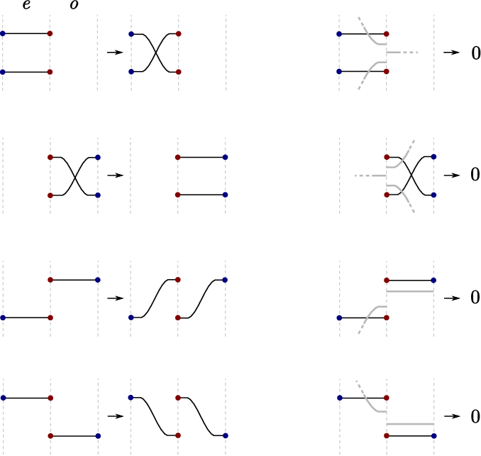
Refer to caption
Figure 14. The map ∂m\partial_{m} along a vertical line with an even piece to the left and an odd piece to the right. For the opposite case, one can simply reflect all diagrams about a vertical line and swap the colors of the dots. Left: The map ∂m\partial_{m} counts four types of exchanges (along the vertical line separating two adjacent pieces) of pairs of black strands, subject to a condition drawn to the right. Right: For a fixed pair of black strands, if there is a black or a red strand in the same relative position to the pair as one of the displayed grey strands, we do not exchange.

Last, we define a map

δL:CT~(𝕋)→A(−∂0𝒯)⊗CT~(𝕋)\delta^{L}:\widetilde{\rm{CT}}(\mathbb{T})\to A(-\partial^{0}\mathcal{T})\otimes\widetilde{\rm{CT}}(\mathbb{T})

as follows. First, we represent a non-zero generator a⊗xa\otimes x for A(−∂0𝒯)⊗CT~(𝕋)A(-\partial^{0}\mathcal{T})\otimes\widetilde{\rm{CT}}(\mathbb{T}) diagrammatically by gluing a diagram for aa to the left of a diagram for xx. Left (resp. right) multiplication is given by concatenating with the leftmost (resp. rightmost) piece of the diagram for a⊗xa\otimes x and scaling horizontally; the differential is given as the sum ∂++∂−+∂m\partial_{+}+\partial_{-}+\partial_{m} of maps defined as above, where we treat the leftmost piece (the diagram for aa) as even. For a generator xx, δL​(x)\delta^{L}(x) is the sum of all generators a⊗ya\otimes y whose diagram can be obtained by gluing a diagram for e0D​(x)e_{0}^{D}(x) (treated as an even diagram) to the left of a diagram for xx, and exchanging two endpoints of black strands that lie on the gluing line, as in the definition of ∂m\partial_{m}. See Figure 15 for an example.

\labellist\pinlabel

δL\delta^{L} at -10 30 \pinlabel⋯\cdots at 82 30 \pinlabel== at 99 30 \pinlabel apply ​∂m here\textrm{ apply }\partial_{m}\textrm{ here} at 160 -27 \pinlabel↑\uparrow at 156 -13 \pinlabel⋯\cdots at 235 30 \pinlabel== at 252 30 \pinlabel⋯\cdots at 386 30 \pinlabel++ at 402 30 \pinlabel⋯\cdots at 533 30 \endlabellist   Refer to caption

Figure 15. The map δL\delta^{L} applied to the generator from Figure 11.
Definition 3.4.1.

Given a tangle decomposition 𝕋\mathbb{T}, we give the (I(−∂0𝒯),I(∂1𝒯))(I(-\partial^{0}\mathcal{T}),I(\partial^{1}\mathcal{T})) bimodule of Definition 3.3.2 the structure of a type 𝐷𝐴\mathit{DA} bimodule over (A(−∂0𝒯),A(∂1𝒯))(A(-\partial^{0}\mathcal{T}),A(\partial^{1}\mathcal{T})) using the following structure maps: let δi1=0\delta_{i}^{1}=0 for i>2i>2, define

δ11:CT~(𝕋)→A(−∂0𝒯)⊗CT~(𝕋)\delta_{1}^{1}:\widetilde{\rm{CT}}(\mathbb{T})\to A(-\partial^{0}\mathcal{T})\otimes\widetilde{\rm{CT}}(\mathbb{T})

on generators by

δ11​(x)=e0D​(x)⊗∂(x)+δL​(x),\delta_{1}^{1}(x)=e_{0}^{D}(x)\otimes\partial(x)+\delta^{L}(x),

and define

δ21:CT~(𝕋)⊗A(∂1𝒯)→A(−∂0𝒯)⊗CT~(𝕋)\delta_{2}^{1}:\widetilde{\rm{CT}}(\mathbb{T})\otimes A(\partial^{1}\mathcal{T})\to A(-\partial^{0}\mathcal{T})\otimes\widetilde{\rm{CT}}(\mathbb{T})

on generators by

δ21​(x⊗a)=e0D​(x)⊗x​a.\delta_{2}^{1}(x\otimes a)=e_{0}^{D}(x)\otimes xa.

By Section 5.2. of [PV16a], the above structure is indeed a type 𝐷𝐴\mathit{DA} bimodule. Define the weight of a generator xx of CT~​(𝕋)\widetilde{\rm{CT}}(\mathbb{T}) just as we did for a generator of A⁡(P)A(P), so that |x|=|e1A​(x)||x|=|e_{1}^{A}(x)|. The bimodule CT~​(𝕋)\widetilde{\rm{CT}}(\mathbb{T}) decomposes as a I(−∂0𝒯)I(-\partial^{0}\mathcal{T}), I⁡(∂1𝒯)I(\partial^{1}\mathcal{T}) bimodule as

CT~​(𝕋)=⨁k=0max⁡{|∂0𝒯|,|∂1𝒯|}+1CT~k​(𝕋),\widetilde{\rm{CT}}(\mathbb{T})=\bigoplus_{k=0}^{\max\{|\partial^{0}\mathcal{T}|,|\partial^{1}\mathcal{T}|\}+1}\widetilde{\rm{CT}}_{k}(\mathbb{T}),

where CT~k​(𝕋)\widetilde{\rm{CT}}_{k}(\mathbb{T}) is the subspace of elements of weight kk.

Note that by forgetting the “right map” ⋅\cdot, the “left map” ∂L\partial^{L}, or both, we can view CT~​(𝕋)\widetilde{\rm{CT}}(\mathbb{T}) as a left type DD structure with δ1=δ11\delta^{1}=\delta_{1}^{1}, a right type AA structure with structure maps m1=∂m_{1}=\partial, m2=⋅m_{2}=\cdot, and mi=0m_{i}=0 for i>2i>2, or a chain complex with differential ∂\partial.

For any of the above four types of structures, the Maslov grading MM is the homological grading, and 22 times the Alexander grading AA is the internal grading.

3.5. Invariance, pairing, and relation to knot Floer homology

To state precise theorems below, we define the size |𝕋||\mathbb{T}| of a tangle decomposition 𝕋\mathbb{T} as one half of the sum ←(p)+→(p){\color[rgb]{1,0,0}{\leftarrow}}(p)+{\color[rgb]{1,0,0}{\rightarrow}}(p), taken over all even and odd pieces pp of the decomposition.

Up to a factor that depends on the size of the chosen decomposition, tangle Floer homology is an invariant of the topological tangle 𝒯\mathcal{T}.

Theorem 3.5.1 (Invariance, cf. [PV16a, Theorem 5.3]).

If 𝕋′\mathbb{T}^{\prime} and 𝕋′′\mathbb{T}^{\prime\prime} are two decompositions for a tangle 𝒯\mathcal{T} with |𝕋′|≥|𝕋′′||\mathbb{T}^{\prime}|\geq|\mathbb{T}^{\prime\prime}|, then there is a bigraded 𝐷𝐴\mathit{DA} homotopy equivalence

CT~​(𝕋′)≃CT~​(𝕋′′)⊗(𝔽2⊕(𝔽2​[1]​{2}))⊗(|𝕋′|−|𝕋′′|)\widetilde{\rm{CT}}(\mathbb{T}^{\prime})\simeq\widetilde{\rm{CT}}(\mathbb{T}^{\prime\prime})\otimes(\mathbb{F}_{2}\oplus(\mathbb{F}_{2}[1]\{2\}))^{\otimes(|\mathbb{T}^{\prime}|-|\mathbb{T}^{\prime\prime}|)}

Further, CT~\widetilde{\rm{CT}} is functorial under composition (this follows automatically from the definition of CT~\widetilde{\rm{CT}}; see also [PV16a, Definition 5.2]).

Theorem 3.5.2 (Pairing).

If 𝕋1\mathbb{T}_{1} and 𝕋2\mathbb{T}_{2} are decompositions for tangles 𝒯1\mathcal{T}_{1} and 𝒯2\mathcal{T}_{2} with ∂1𝒯1=−∂0𝒯2\partial^{1}\mathcal{T}_{1}=-\partial^{0}\mathcal{T}_{2}, then CT~​(𝕋)\widetilde{\rm{CT}}(\mathbb{T}) is bigraded isomorphic to CT~​(𝕋1)⊠CT~​(𝕋2)\widetilde{\rm{CT}}(\mathbb{T}_{1})\boxtimes\widetilde{\rm{CT}}(\mathbb{T}_{2}) as type 𝐷𝐴\mathit{DA} structures, where 𝕋\mathbb{T} is the decomposition for 𝒯1∘𝒯2\mathcal{T}_{1}\circ\mathcal{T}_{2} that is the concatenation of the two decompositions 𝕋1\mathbb{T}_{1} and 𝕋2\mathbb{T}_{2}.

In the case of a closed link, tangle Floer homology agrees with knot Floer homology HFK^​(𝒦){\rm{\widehat{HFK}}}(\mathcal{K}), the bigraded invariant of knots and links defined, in its various versions, in [OS04, Ras03, MOST07, OS08]. As defined here, given a link decomposition 𝕋\mathbb{T}, CT~​(𝕋)≅CT~0​(𝕋)⊕CT~1​(𝕋)\widetilde{\rm{CT}}(\mathbb{T})\cong\widetilde{\rm{CT}}_{0}(\mathbb{T})\oplus\widetilde{\rm{CT}}_{1}(\mathbb{T}). The two summands CT~0​(𝕋)\widetilde{\rm{CT}}_{0}(\mathbb{T}) and CT~1​(𝕋)\widetilde{\rm{CT}}_{1}(\mathbb{T}) are bigraded homotopy equivalent (for experts: each of CT~0​(𝕋)\widetilde{\rm{CT}}_{0}(\mathbb{T}) and CT~1​(𝕋)\widetilde{\rm{CT}}_{1}(\mathbb{T}) corresponds to a certain Heegaard diagram for the link for 𝕋\mathbb{T}), and the relation to knot Floer homology can be stated in terms of either.

Theorem 3.5.3 (cf. [PV16a, Theorem 6.1, item (4) of Corollary 12.5]).

Suppose that 𝕋\mathbb{T} is a decomposition for a closed link 𝒦\mathcal{K} with |𝒦||\mathcal{K}| connected components. Then there is a bigraded homotopy equivalence of complexes

CT~0​(𝕋)≃CT~1​(𝕋)≃HFK^​(𝒦)⊗(𝔽2⊕(𝔽2​[1]​{2}))⊗(|𝕋|−|𝒦|)⊗(𝔽2⊕(𝔽2​[1]​{0})).\widetilde{\rm{CT}}_{0}(\mathbb{T})\simeq\widetilde{\rm{CT}}_{1}(\mathbb{T})\simeq{\rm{\widehat{HFK}}}(\mathcal{K})\otimes(\mathbb{F}_{2}\oplus(\mathbb{F}_{2}[1]\{2\}))^{\otimes(|\mathbb{T}|-|\mathcal{K}|)}\otimes(\mathbb{F}_{2}\oplus(\mathbb{F}_{2}[1]\{0\})).

3.6. Dictionary

Section 3 can be thought of as a “user’s guide” to [PV16a]; the terminology and notation here are different from [PV16a] to ease readability. Below is a (non-comprehensive) list of the major correspondences between this section and [PV16a, Section 3].

Here In [PV16a]
a tangle decomposition an alternating sequence of shadows and mirror-
𝕋=(𝒯1,…,𝒯k)\mathbb{T}=(\mathcal{T}_{1},\ldots,\mathcal{T}_{k}) shadows 𝓟=(𝒫1∗,𝒫2,…,𝒫2​k−1∗,𝒫2​k)\boldsymbol{\mathcal{P}}=(\mathcal{P}_{1}^{*},\mathcal{P}_{2},\ldots,\mathcal{P}_{2k-1}^{*},\mathcal{P}_{2k})
the ii-th even piece in 𝕋\mathbb{T} the shadow 𝒫2​i\mathcal{P}_{2i}
(drawn over white background color)
the ii-th odd piece in 𝕋\mathbb{T} the mirror-shadow 𝒫2​i−1∗\mathcal{P}_{2i-1}^{*}
(drawn over grey background color)
⟶\longrightarrow in an even piece - - - - on 𝒫\mathcal{P}
⟵\longleftarrow in an odd piece - - - - on 𝒫∗\mathcal{P}^{*}
⟵\longleftarrow in an even piece ====\mathrel{\mkern-3.0mu}=\mathrel{\mkern-3.0mu}= on 𝒫\mathcal{P}
⟶\longrightarrow in an odd piece ====\mathrel{\mkern-3.0mu}=\mathrel{\mkern-3.0mu}= on 𝒫∗\mathcal{P}^{*}
P⊂{±1}nP\subset\{\pm 1\}^{n} ϵ∈(2{±})n\epsilon\in(2^{\{\pm\}})^{n}
ViV_{i} 𝐚\mathbf{a} for 𝒫2​i\mathcal{P}_{2i} and P2​i+1∗P_{2i+1}^{*} (called 𝐚i\mathbf{a}_{i} below)
WiW_{i} 𝐛\mathbf{b} for 𝒫2​i−1∗\mathcal{P}_{2i-1}^{*} and 𝒫2​i\mathcal{P}_{2i} (called 𝐛i\mathbf{b}_{i} below)

Further, fix a generator xx of 𝕋\mathbb{T}, where 𝕋\mathbb{T} is as above, and label the respective partial bijections as x2​i−1:Vi−1→Wix_{2i-1}:V_{i-1}\to W_{i} and x2​i:Wi→Vix_{2i}:W_{i}\to V_{i}. We have the following correspondences.

Here In [PV16a]
x2​i:Wi→Vix_{2i}:W_{i}\to V_{i} (S2​i,T2​i,ϕ2​i)(S_{2i},T_{2i},\phi_{2i}), where S2​i⊂𝐛i,T2​i⊂𝐚iS_{2i}\subset\mathbf{b}_{i},T_{2i}\subset\mathbf{a}_{i} and
ϕ2​i:S2​i→T2​i\phi_{2i}:S_{2i}\to T_{2i} is a bijection
x2​i−1:Vi−1→Wix_{2i-1}:V_{i-1}\to W_{i} (S2​i−1,T2​i−1,ϕ2​i−1)∗(S_{2i-1},T_{2i-1},\phi_{2i-1})^{*}, where S2​i−1⊂𝐛i−1S_{2i-1}\subset\mathbf{b}_{i-1}, T2​i−1⊂𝐚iT_{2i-1}\subset\mathbf{a}_{i}
and ϕ2​i−1:S2​i−1→T2​i−1\phi_{2i-1}:S_{2i-1}\to T_{2i-1} is a bijection
a black strand for xix_{i} a pair (s,ϕ​s)(s,\phi s) for s∈Sis\in S_{i}
𝐬1A​(x){\bf s}^{A}_{1}(x) T2​kT_{2k}
𝐬0D​(x){\bf s}^{D}_{0}(x) 𝐚0∖T0\mathbf{a}_{0}\setminus T_{0}

4. Proofs of the main results

4.1. The Grothendieck group of A⁡(P)A(P)

If an element x∈A⁡(P)x\in A(P) satisfies e𝐭​x=δ𝐬,𝐭​xe_{{\bf t}}x=\delta_{{\bf s},{\bf t}}x, we say that xx has left I⁡(P)I(P)-degree equal to 𝐬{\bf s}. We define right I⁡(P)I(P)-degree as well as such degrees for elements of A⁡(P)A(P)-modules analogously.

Let P∈{±1}nP\in\{\pm 1\}^{n} be a sign sequence, A⁡(P)A(P) the corresponding tangle Floer dg algebra, and I⁡(P)I(P) the ring of idempotents in A⁡(P)A(P). For a subset 𝐬⊆[n]{\bf s}\subseteq[n], let e𝐬e_{{\bf s}} be the corresponding primitive idempotent. Since I⁡(P)≅𝔽2⊕2n+1I(P)\cong\mathbb{F}_{2}^{\oplus 2^{n+1}} with zero differential, we have

K0​(I⁡(P))≅ℤ2n+1⊗ℤℤ⁡[q±1].K_{0}(I(P))\cong\mathbb{Z}^{2^{n+1}}\otimes_{\mathbb{Z}}\mathbb{Z}[q^{\pm 1}]. (39)

A free ℤ⁡[q±1]\mathbb{Z}[q^{\pm 1}]-basis for K0​(I​(P))K_{0}(I(P)) is given by {[I⁡(P)​e𝐬]∣𝐬⊆[n]}\{[I(P)e_{{\bf s}}]\mid{\bf s}\subseteq[n]\}. We call this the primitive basis of K0​(I​(P))K_{0}(I(P)).

Let VV be a bigraded 𝔽2\mathbb{F}_{2}-vector space and write Vi,jV_{i,j} for the part of VV in homological (Maslov) degree i∈ℤi\in\mathbb{Z} and internal (twice Alexander) degree j∈ℤj\in\mathbb{Z}. Suppose ⨁i∈ℤVi,j\bigoplus_{i\in\mathbb{Z}}V_{i,j} is finite dimensional for each j∈ℤj\in\mathbb{Z}. The graded Euler characteristic of VV is the formal series

χ⁡(V)=∑i,j∈ℤ(−1)i​qj​dim𝔽2(Vi,j).\chi(V)=\sum_{i,j\in\mathbb{Z}}(-1)^{i}q^{j}\dim_{\mathbb{F}_{2}}(V_{i,j}). (40)

In all our cases of interest, χ⁡(V)\chi(V) will be a polynomial in q±1q^{\pm 1}.

Let 𝔽2A​{𝐬}\prescript{A}{}{\mathbb{F}_{2}\{{\bf s}\}} be the one-dimensional left type D\mathit{D} structure over AA spanned by a homogeneous generator x𝐬x_{\bf s} of Maslov degree 00, Alexander degree 00, I⁡(P)I(P)-degree 𝐬{\bf s}, and satisfying δ1​(x𝐬)=0\delta^{1}(x_{\bf s})=0. The corresponding left type A\mathit{A} module

A⊠𝔽2A​{𝐬}≅A​e𝐬.A\boxtimes\prescript{A}{}{\mathbb{F}_{2}\{{\bf s}\}}\cong Ae_{{\bf s}}. (41)
Proposition 4.1.1.

Let P∈{±1}nP\in\{\pm 1\}^{n}.

  1. (1)

    Then the Grothendieck group of the compact derived category of left dg modules over A⁡(P)A(P) is

    K0​(A⁡(P))≅ℤ2n+1⊗ℤ⁡[q±1].K_{0}(A(P))\cong\mathbb{Z}^{2^{n+1}}\otimes\mathbb{Z}[q^{\pm 1}]. (42)
  2. (2)

    If MA⁡(P)\prescript{}{A(P)}{M} is a compact cofibrant dg module over A⁡(P)A(P), then [M]=∑𝐬⊆[n]c𝐬​[A⁡(P)​e𝐬][M]=\sum_{{\bf s}\subseteq[n]}c_{{\bf s}}[A(P)e_{{\bf s}}] for certain constants c𝐬∈ℤ⁡[q±1]c_{{\bf s}}\in\mathbb{Z}[q^{\pm 1}]. The set {[A​e𝐬]∣𝐬⊆[n]}\{[Ae_{{\bf s}}]\mid{\bf s}\subseteq[n]\} is a basis of K0​(A​(P))K_{0}(A(P)) over ℤ⁡[q±1]\mathbb{Z}[q^{\pm 1}].

  3. (3)

    Under the quasi-equivalence of Proposition 2.2.1, we can view the class of a bounded left type D\mathit{D} structure as an element of K0​(A​(P))K_{0}(A(P)). Under this identification, for any bounded left DD structure NA⁡(P)\prescript{A(P)}{}{N},

    [NA⁡(P)]=∑𝐬⊆[n]χ⁡(e𝐬​N)​[A⁡(P)​e𝐬].[\prescript{A(P)}{}{N}]=\sum_{{\bf s}\subseteq[n]}\chi(e_{{\bf s}}N)[A(P)e_{{\bf s}}]. (43)
Proof.

The idea of the proof is analogous to that of [Pet18, Theorem 21]. We give the details here for completeness.

The dg (I⁡(P),A⁡(P))(I(P),A(P))-bimodule A⁡(P)A(P) induces a derived tensor functor (as in Subsection 2.2) 𝒟⁡(A⁡(P))→𝒟⁡(I⁡(P))\mathcal{D}(A(P))\to\mathcal{D}(I(P)). This functor takes a dg module MM over A⁡(P)A(P) to M/(A​(P)+​M)M/(A(P)_{+}M). In particular, for a primitive idempotent e𝐬e_{{\bf s}}, the induced map on Grothendieck groups takes [A⁡(P)​e𝐬][A(P)e_{{\bf s}}] to the primitive basis vector [I⁡(P)​e𝐬][I(P)e_{{\bf s}}]. It follows that

{[A⁡(P)​e𝐬]∣𝐬⊆[n]}\{[A(P)e_{{\bf s}}]\mid{\bf s}\subseteq[n]\}

is a ℤ⁡[q±1]\mathbb{Z}[q^{\pm 1}]-linearly independent set in K0​(A​(P))K_{0}(A(P)).

It suffices, then, to express the symbol of any compact cofibrant dg module over A⁡(P)A(P) as a ℤ⁡[q±1]\mathbb{Z}[q^{\pm 1}]-linear combination of symbols of the form [A⁡(P)​e𝐬][A(P)e_{{\bf s}}]. By Proposition 2.2.1, it suffices to consider modules of the form A⁡(P)⊠NA(P)\boxtimes N, where NN is a bounded left type D\mathit{D} structure over A⁡(P)A(P).

Given such a module, choose an 𝔽2\mathbb{F}_{2}-basis x1,…,xrx_{1},\ldots,x_{r} for NN such that xi=e0D​(xi)​xix_{i}=e_{0}^{D}(x_{i})x_{i} for each ii. By boundedness, we can choose jj such that δ1​(xj)=0\delta^{1}(x_{j})=0. In the sum

d⁡(a⊗xj)=∑k=1∞[(mk⊗idN)∘(idM⊗δk−1)]​(a⊗xj),d(a\otimes x_{j})=\sum_{k=1}^{\infty}\left[(m_{k}\otimes\id_{N})\circ(\id_{M}\otimes\delta^{k-1})\right](a\otimes x_{j}),

only the k=1k=1 term survives. This term equals m1​(a)⊗xj=d⁡(a)⊗xjm_{1}(a)\otimes x_{j}=d(a)\otimes x_{j}. Hence A⁡(P)⊗xjA(P)\otimes x_{j} is a dg submodule isomorphic to A⁡(P)​exj​[−M⁡(xj)]​{−2​A​(xj)}A(P)e_{x_{j}}[-M(x_{j})]\{-2A(x_{j})\}, where exje_{x_{j}} is the primitive idempotent with the same I⁡(P)I(P)-degree as xjx_{j}. Write Mj=A⁡(P)​exj​[−M⁡(xj)]​{−2​A​(xj)}M_{j}=A(P)e_{x_{j}}[-M(x_{j})]\{-2A(x_{j})\} for short, and let ι\iota be the inclusion of this submodule. Then the triangle

Mj\textstyle{M_{j}\ignorespaces\ignorespaces\ignorespaces\ignorespaces}ι\scriptstyle{\iota}A⁡(P)⊠N\textstyle{A(P)\boxtimes N\ignorespaces\ignorespaces\ignorespaces\ignorespaces}C⁡(ι)\textstyle{C(\iota)\ignorespaces\ignorespaces\ignorespaces\ignorespaces}Mj​[1]\textstyle{M_{j}[1]}

is isomorphic to a distinguished triangle, so

[A⁡(P)⊠N]=[Mj]+[(A⁡(P)⊠N)/Mj].[A(P)\boxtimes N]=[M_{j}]+[(A(P)\boxtimes N)/M_{j}].

We have [Mj]=(−1)M⁡(xj)​q−2​A​(xj)​[A⁡(P)​exj][M_{j}]=(-1)^{M(x_{j})}q^{-2A(x_{j})}[A(P)e_{x_{j}}]. So by induction on the dimension of NN, [A⁡(P)⊠N][A(P)\boxtimes N] is a sum of terms of the form ±qk​[A⁡(P)​e𝐬]\pm q^{k}[A(P)e_{{\bf s}}]. So K0​(A​(P))K_{0}(A(P)) is a free ℤ⁡[q±1]\mathbb{Z}[q^{\pm 1}]-module with a basis given by the 2n+12^{n+1} symbols {[A​e𝐬]∣𝐬⊆[n]}\{[Ae_{{\bf s}}]\mid{\bf s}\subseteq[n]\}.

Equation (43) follows immediately from the above analysis and the quasi-equivalence of Proposition 2.2.1. ∎

Proposition 4.1.1 implies the first half of Theorem A of the Introduction.

We call {[A​e𝐬]∣𝐬⊆[n]}\{[Ae_{{\bf s}}]\mid{\bf s}\subseteq[n]\} the primitive basis of K0​(A)K_{0}(A). When discussing elements of and linear maps between Grothendieck groups of A⁡(P)A(P)’s, our default will be to use this basis. We call a𝐬a_{\bf s} the “𝐬{\bf s} component” of an element

∑𝐬a𝐬​[A​e𝐬]∈K0​(A),\sum_{{\bf s}}a_{\bf s}[Ae_{{\bf s}}]\in K_{0}(A),

and if X:K0​(A⁡(P))→K0​(A⁡(P′))X:K_{0}(A(P))\to K_{0}(A(P^{\prime})) is a ℤ⁡[q±1]\mathbb{Z}[q^{\pm 1}]-linear map and

X⁡([A⁡(P)​e𝐭])=∑𝐬X𝐬,𝐭​[A⁡(P′)​e𝐬],X([A(P)e_{{\bf t}}])=\sum_{{\bf s}}X_{{\bf s},{\bf t}}[A(P^{\prime})e_{{\bf s}}],

we call X𝐬,𝐭X_{{\bf s},{\bf t}} the “(𝐬,𝐭)({\bf s},{\bf t}) matrix entry” of XX. In our main construction, XX will usually be the linear map induced by the derived (or box) tensor product with some bimodule. In the case of a type 𝐷𝐴\mathit{DA} bimodule, the computation of the components X𝐬,𝐭X_{{\bf s},{\bf t}} is just a graded dimension count, as we presently explain.

Proposition 4.1.2.

Let MM be a bounded type 𝐷𝐴\mathit{DA} bimodule over (A⁡(P′),A⁡(P))(A(P^{\prime}),A(P)) for two sign sequences P,P′P,P^{\prime}. MM induces a homomorphism

[M⊠−]:K0(A(P))→K0(A(P′))[M\boxtimes-]:K_{0}(A(P))\to K_{0}(A(P^{\prime}))

via the rule

[M⊠−]:[M′A⁡(P)]↦[A(P′)⊠MA⁡(P)A⁡(P′)⊗~M′A⁡(P)].[M\boxtimes-]:[\prescript{}{A(P)}{M^{\prime}}]\mapsto[A(P^{\prime})\boxtimes\prescript{A(P^{\prime})}{}{M}_{A(P)}\mathbin{\widetilde{\otimes}}\prescript{}{A(P)}{M^{\prime}}]. (44)

Using the quasi-equivalence of Proposition 2.2.1, this rule can also be stated as

[M⊠−]:[NA⁡(P)]↦[MA⁡(P)A⁡(P′)⊠NA⁡(P)].[M\boxtimes-]:[\prescript{A(P)}{}{N}]\mapsto[\prescript{A(P^{\prime})}{}{M}_{A(P)}\boxtimes\prescript{A(P)}{}{N}]. (45)

This homomorphism has matrix entries

[M⊠−]𝐬,𝐭=χ(e𝐬Me𝐭).[M\boxtimes-]_{{\bf s},{\bf t}}=\chi(e_{{\bf s}}Me_{{\bf t}}). (46)
Proof.

That MM induces a homomorphism via (44) follows from the quasi-equivalence of Proposition 2.2.1 and the fact that the derived tensor product with a dg module induces a homomorphism of Grothendieck groups (cf. Section 2.2). Again by Proposition 2.2.1, the rules (44) and (45) are equivalent. Abbreviating A⁡(P)A(P) by AA and A⁡(P′)A(P^{\prime}) by A′A^{\prime}, the matrix entry description is an easy computation:

[MAA′⊗~A⊠𝔽2A​{𝐬}]​          (41)                ​[MAA′⊗~A​e𝐬]=∑𝐭[A′⊠e𝐭​M​e𝐬]=∑𝐭χ⁡(e𝐭​M​e𝐬)​[A′​e𝐭].∎[\prescript{A^{\prime}}{}{M}_{A}\mathbin{\widetilde{\otimes}}A\boxtimes\prescript{A}{}{\mathbb{F}_{2}\{{\bf s}\}}]\lx@xy@svg{\hbox{\raise 2.5pt\hbox{\kern 37.73973pt\hbox{\ignorespaces\ignorespaces\ignorespaces{}{}\ignorespaces\ignorespaces\ignorespaces\ignorespaces{}\ignorespaces{\hbox{\hbox{\kern 0.0pt\raise 1.0pt\hbox{\lx@xy@droprule}}\hbox{\kern 0.0pt\raise-1.0pt\hbox{\lx@xy@droprule}}}}\ignorespaces\ignorespaces\ignorespaces{\hbox{\kern-37.73973pt\raise 6.1111pt\hbox{{}\hbox{\kern 0.0pt\raise 0.0pt\hbox{\hbox{\kern 3.0pt\hbox{\hbox{\kern 0.0pt\raise-1.75pt\hbox{$\scriptstyle{\eqref{eqn-one-dim-type-D}}$}}}\kern 3.0pt}}}}}}\ignorespaces{}\ignorespaces{\hbox{\hbox{\kern 0.0pt\raise 1.0pt\hbox{\lx@xy@droprule}}\hbox{\kern 0.0pt\raise-1.0pt\hbox{\lx@xy@droprule}}}}{\hbox{\hbox{\kern 0.0pt\raise 1.0pt\hbox{\lx@xy@droprule}}\hbox{\kern 0.0pt\raise-1.0pt\hbox{\lx@xy@droprule}}}}\ignorespaces}}}}[\prescript{A^{\prime}}{}{M}_{A}\mathbin{\widetilde{\otimes}}Ae_{{\bf s}}]=\sum_{\bf t}[A^{\prime}\boxtimes e_{{\bf t}}Me_{{\bf s}}]=\sum_{\bf t}\chi(e_{{\bf t}}Me_{{\bf s}})[A^{\prime}e_{{\bf t}}].\qed
Corollary 4.1.3.

Let 𝒯\mathcal{T} be a tangle with decomposition 𝕋\mathbb{T}. Then the matrix entries of the homomorphism [CT~(𝕋)⊠−]:K0(A(∂1𝒯))→K0(A(−∂0𝒯))[\widetilde{\rm{CT}}(\mathbb{T})\boxtimes-]:K_{0}(A(\partial^{1}\mathcal{T}))\to K_{0}(A(-\partial^{0}\mathcal{T})) are given by

[CT~(𝕋)⊠−]𝐬,𝐭=χ(e𝐬CT~(𝕋)e𝐭).[\widetilde{\rm{CT}}(\mathbb{T})\boxtimes-]_{{\bf s},{\bf t}}=\chi(e_{{\bf s}}\widetilde{\rm{CT}}(\mathbb{T})e_{{\bf t}}). (47)

We will abbreviate [M⊠−]𝐬,𝐭[M\boxtimes-]_{{\bf s},{\bf t}} as [M]𝐬,𝐭[M]_{{\bf s},{\bf t}} below.

4.2. The action of CT~​(𝕋)\widetilde{\rm{CT}}(\mathbb{T}) on the Grothendieck group

In this subsection, we compute the symbol [CT~​(𝕋)][\widetilde{\rm{CT}}(\mathbb{T})] for any tangle decomposition by induction. Our base case is an explicit computation for the smallest elementary tangles. Then we induct by computing the result of adding a horizontal strand above or below a decomposition 𝕋\mathbb{T}.

Remark.

All matrices below are with respect to the primitive basis {[A⁡(P)​e𝐬]∣I⊆[n]}\{[A(P)e_{{\bf s}}]\mid I\subseteq[n]\} of K0​(A​(P))K_{0}(A(P)) as defined in the previous subsection. We give this basis the reverse lexicographic order with respect to the alphabet 0<1<…<n0<1<\ldots<n: a subset 𝐬{\bf s} is treated as a word w⁡(𝐬)w({\bf s}) spelled in decreasing order, and we say 𝐬<𝐭{\bf s}<{\bf t} if w⁡(𝐬)<w⁡(𝐭)w({\bf s})<w({\bf t}) in the lexicographic (“alphabetical”) order. For example, when |P|=2|P|=2, the ordering is

e∅<e{0}<e{1}<e{0,1}<e{2}<e{0,2}<e{1,2}<e{0,1,2}.e_{\emptyset}\enskip<\enskip e_{\{0\}}\enskip<\enskip e_{\{1\}}\enskip<\enskip e_{\{0,1\}}\enskip<\enskip e_{\{2\}}\enskip<\enskip e_{\{0,2\}}\enskip<\enskip e_{\{1,2\}}\enskip<\enskip e_{\{0,1,2\}}.

Suppose |P|=n|P|=n and P′P^{\prime} is the sign subsequence which omits the last entry of PP. The ordered primitive basis for PP has length 2n+12^{n+1}. Its first 2n2^{n} elements are exactly the ordered primitive basis for P′P^{\prime}, and the (2n+i)(2^{n}+i)-th element is 𝐬⊔{n}{\bf s}\sqcup\{n\}, where 𝐬{\bf s} is the ii-th element of either ordered basis.

From now on, using the previous remark and Proposition 4.1.1, we will identify

K0​(A⁡(P))⊗ℤ⁡[q±1]ℂ⁡(q)≅VP⊗L⁡(λP)[A⁡(P)​e𝐬]↔ℓj1∧…∧ℓjr,\begin{split}K_{0}(A(P))\otimes_{\mathbb{Z}[q^{\pm 1}]}\mathbb{C}(q)&\cong V_{P}\otimes L(\lambda_{P})\\ [A(P)e_{{\bf s}}]&\leftrightarrow\ell_{j_{1}}\wedge\ldots\wedge\ell_{j_{r}},\end{split} (48)

where {j1<…<jr}=[n]∖𝐬\{j_{1}<\ldots<j_{r}\}=[n]\setminus{\bf s}. Note that this identification is order preserving.

Although by invariance it suffices to compute only one of the eight possible oriented crossings, we provide the matrices for all crossings (but provide details for only one).

In the discussion below, let P=(P1,P2)P=(P_{1},P_{2}) be a sign sequence of length 22.

Let 𝚎P\mathtt{e}_{P} denote the elementary tangle that is an e-crossing of two strands such that ∂1(𝚎P)=P\partial^{1}(\mathtt{e}_{P})={P}.

Let 𝚘P\mathtt{o}_{P} denote the elementary tangle that is an o-crossing of two strands such that −∂0(𝚘P)=P-\partial^{0}(\mathtt{o}_{P})=P.

With this notation, 𝕋=(𝚎P,𝚘P)\mathbb{T}=(\mathtt{e}_{P},\mathtt{o}_{P}) is a decomposition for the tangle 𝒯=I×(P2,P1)\mathcal{T}=I\times(P_{2},P_{1}), and (𝚘P,𝚎P)(\mathtt{o}_{P},\mathtt{e}_{P}) is a decomposition for the tangle I×PI\times{P}.

To compute the action of CT~​(𝕋)\widetilde{\rm{CT}}(\mathbb{T}) on K0K_{0}, we just need to compute the bigradings of the generators, and take the graded Euler characteristic. Recall that the primitive idempotents are of form e𝐬e_{{\bf s}}, where 𝐬⊆{0,1,2}{\bf s}\subseteq\{0,1,2\}, and that a generator xx for CT~​(𝕋)\widetilde{\rm{CT}}(\mathbb{T}) occupies the black dot at height hh on the left (respectively right) exactly when h∉𝐬0D​(x)h\notin{\bf s}^{D}_{0}(x) (respectively h∈𝐬1A​(x)h\in{\bf s}^{A}_{1}(x)). For ease of reading, we give the matrices for each weight separately.

We discuss the computation of [CT~2​(𝚎+⁣+)]{0,2},{1,2}[\widetilde{\rm{CT}}_{2}(\mathtt{e}_{++})]_{\{0,2\},\{1,2\}} below. Since the induced order on subsets of size 22 is {0,1}<{0,2}<{1,2}\enskip\{0,1\}\enskip<\enskip\{0,2\}\enskip<\enskip\{1,2\}, this corresponds to the (2,3)(2,3) entry of the matrix for [CT~2​(𝚎+⁣+)][\widetilde{\rm{CT}}_{2}(\mathtt{e}_{++})].

The 𝐷𝐴\mathit{DA} bimodule CT~​(𝚎+⁣+)\widetilde{\rm{CT}}(\mathtt{e}_{++}) for the crossing 𝚎+⁣+\mathtt{e}_{++} (depicted on the left diagram below) is generated by pairs of partial bijections associated to the right diagram below.

[Uncaptioned image]

The vector space e{0,2}​CT~​(𝚎+⁣+)​e{1,2}e_{\{0,2\}}\widetilde{\rm{CT}}(\mathtt{e}_{++})e_{\{1,2\}} is generated over 𝔽2\mathbb{F}_{2} by the strand diagrams in Figure 16. The formulas from Section 3.3 yield the bigradings listed in Figure 16.

\labellist\pinlabel

(−1,−2)(-1,-2) at 40 -14 \pinlabel(−2,−4)(-2,-4) at 140 -14 \pinlabel(−1,−2)(-1,-2) at 238 -14 \pinlabel(0,0)(0,0) at 335 -14 \pinlabel(−1,−2)(-1,-2) at 435 -14 \pinlabel(0,−2)(0,-2) at 530 -14 \endlabellistRefer to caption

Figure 16. The generators of e{0,2}​CT~​(𝚎+⁣+)​e{1,2}e_{\{0,2\}}\widetilde{\rm{CT}}(\mathtt{e}_{++})e_{\{1,2\}} and their (M,2​A)(M,2A) bigradings.

Thus,

[CT~2​(𝚎+⁣+)]{0,2},{1,2}=χ⁡(e{0,2}​CT~​(𝚎+⁣+)​e{1,2})=∑x​ a generator(−1)M⁡(x)​q2​A​(x)=(1−q−2)2.[\widetilde{\rm{CT}}_{2}(\mathtt{e}_{++})]_{\{0,2\},\{1,2\}}=\chi(e_{\{0,2\}}\widetilde{\rm{CT}}(\mathtt{e}_{++})e_{\{1,2\}})=\sum_{x\textrm{ a generator}}(-1)^{M(x)}q^{2A(x)}=(1-q^{-2})^{2}.

Analogous computations for the remaining weights of CT~​(𝚎+⁣+)\widetilde{\rm{CT}}(\mathtt{e}_{++}) and for the remaining e-crossings yield the matrices in Table 1.

Tangle Diagram Action on K0K_{0}
\labellist\pinlabel 𝚎+⁣+\mathtt{e}_{++} at 28 40 \endlabellist[Uncaptioned image] [Uncaptioned image] =(1−q−2)2​(−q)[CT~1​(𝚎+⁣+)]=(1−q−2)2​(−q100q−1001−q)[CT~2​(𝚎+⁣+)]=(1−q−2)2​(q−1001−q100q−1)[CT~3​(𝚎+⁣+)]=(1−q−2)2​(q−1)\!\begin{aligned} &=(1-q^{-2})^{2}\begin{pmatrix}-q\end{pmatrix}\\ [\widetilde{\rm{CT}}_{1}(\mathtt{e}_{++})]&=(1-q^{-2})^{2}\begin{pmatrix}-q&1&0\\ 0&q^{-1}&0\\ 0&1&-q\end{pmatrix}\\ [\widetilde{\rm{CT}}_{2}(\mathtt{e}_{++})]&=(1-q^{-2})^{2}\begin{pmatrix}q^{-1}&0&0\\ 1&-q&1\\ 0&0&q^{-1}\end{pmatrix}\\ [\widetilde{\rm{CT}}_{3}(\mathtt{e}_{++})]&=(1-q^{-2})^{2}\begin{pmatrix}q^{-1}\end{pmatrix}\end{aligned}
\labellist\pinlabel 𝚎−⁣+\mathtt{e}_{-+} at 28 40 \endlabellist[Uncaptioned image] [Uncaptioned image] =(1−q−2)2​(1)[CT~1​(𝚎−⁣+)]=(1−q−2)2​(1q00100−q−11)[CT~2​(𝚎−⁣+)]=(1−q−2)2​(100−q−11q001)[CT~3​(𝚎−⁣+)]=(1−q−2)2​(1)\!\begin{aligned} &=(1-q^{-2})^{2}\begin{pmatrix}1\end{pmatrix}\\ [\widetilde{\rm{CT}}_{1}(\mathtt{e}_{-+})]&=(1-q^{-2})^{2}\begin{pmatrix}1&q&0\\ 0&1&0\\ 0&-q^{-1}&1\end{pmatrix}\\ [\widetilde{\rm{CT}}_{2}(\mathtt{e}_{-+})]&=(1-q^{-2})^{2}\begin{pmatrix}1&0&0\\ -q^{-1}&1&q\\ 0&0&1\end{pmatrix}\\ [\widetilde{\rm{CT}}_{3}(\mathtt{e}_{-+})]&=(1-q^{-2})^{2}\begin{pmatrix}1\end{pmatrix}\end{aligned}
\labellist\pinlabel 𝚎+⁣−\mathtt{e}_{+-} at 28 40 \endlabellist[Uncaptioned image] [Uncaptioned image] =(1−q−2)2​(1)[CT~1​(𝚎+⁣−)]=(1−q−2)2​(1−q−100100q1)[CT~2​(𝚎+⁣−)]=(1−q−2)2​(100q1−q−1001)[CT~3​(𝚎+⁣−)]=(1−q−2)2​(1)\!\begin{aligned} &=(1-q^{-2})^{2}\begin{pmatrix}1\end{pmatrix}\\ [\widetilde{\rm{CT}}_{1}(\mathtt{e}_{+-})]&=(1-q^{-2})^{2}\begin{pmatrix}1&-q^{-1}&0\\ 0&1&0\\ 0&q&1\end{pmatrix}\\ [\widetilde{\rm{CT}}_{2}(\mathtt{e}_{+-})]&=(1-q^{-2})^{2}\begin{pmatrix}1&0&0\\ q&1&-q^{-1}\\ 0&0&1\end{pmatrix}\\ [\widetilde{\rm{CT}}_{3}(\mathtt{e}_{+-})]&=(1-q^{-2})^{2}\begin{pmatrix}1\end{pmatrix}\end{aligned}
\labellist\pinlabel 𝚎−⁣−\mathtt{e}_{--} at 28 40 \endlabellist[Uncaptioned image] [Uncaptioned image] =(1−q−2)2​(q−1)[CT~1​(𝚎−⁣−)]=(1−q−2)2​(q−1100−q001q−1)[CT~2​(𝚎−⁣−)]=(1−q−2)2​(−q001q−1100−q)[CT~3​(𝚎−⁣−)]=(1−q−2)2​(−q)\!\begin{aligned} &=(1-q^{-2})^{2}\begin{pmatrix}q^{-1}\end{pmatrix}\\ [\widetilde{\rm{CT}}_{1}(\mathtt{e}_{--})]&=(1-q^{-2})^{2}\begin{pmatrix}q^{-1}&1&0\\ 0&-q&0\\ 0&1&q^{-1}\end{pmatrix}\\ [\widetilde{\rm{CT}}_{2}(\mathtt{e}_{--})]&=(1-q^{-2})^{2}\begin{pmatrix}-q&0&0\\ 1&q^{-1}&1\\ 0&0&-q\end{pmatrix}\\ [\widetilde{\rm{CT}}_{3}(\mathtt{e}_{--})]&=(1-q^{-2})^{2}\begin{pmatrix}-q\end{pmatrix}\end{aligned}
Table 1. The action of the crossing bimodules on the Grothendieck group

An elementary tangle trivP=I×P\mathrm{triv}_{P}=I\times{P} acts as a scalar multiple of the identity on K0K_{0},

[CT~​(trivP)]𝐬,𝐭=(1−q−2)2​id.[\widetilde{\rm{CT}}(\mathrm{triv}_{P})]_{{\bf s},{\bf t}}=(1-q^{-2})^{2}\id. (49)

One can see this by computing [CT~​(id())][\widetilde{\rm{CT}}(\id_{()})], and then applying Proposition 4.2.1 (below).

By invariance (Theorem 3.5.1), since (𝚘P,𝚎P)(\mathtt{o}_{P},\mathtt{e}_{P}) is isotopic to trivP\mathrm{triv}_{P}, we have

CT~​(𝚘P,𝚎P)≃CT~​(trivP)⊗(𝔽2⊕𝔽2​[1]​{2})⊗2,\widetilde{\rm{CT}}(\mathtt{o}_{P},\mathtt{e}_{P})\simeq\widetilde{\rm{CT}}(\mathrm{triv}_{P})\otimes(\mathbb{F}_{2}\oplus\mathbb{F}_{2}[1]\{2\})^{\otimes 2},

so [CT~​(𝚘P,𝚎P)]=(1−q−2)4​id[\widetilde{\rm{CT}}(\mathtt{o}_{P},\mathtt{e}_{P})]=(1-q^{-2})^{4}\id. Then

[CT~i​(𝚘P)]=(1−q−2)4​[CT~i​(𝚎P)]−1.[\widetilde{\rm{CT}}_{i}(\mathtt{o}_{P})]=(1-q^{-2})^{4}[\widetilde{\rm{CT}}_{i}(\mathtt{e}_{P})]^{-1}.

Alternatively, one can compute the Euler characteristic explicitly.

Let 𝚌𝚞𝚙+⁣−\mathtt{cup}_{+-} or 𝚌𝚞𝚙−⁣+\mathtt{cup}_{-+} denote the elementary tangle that is a single cup such that ∂0(𝚌𝚞𝚙+⁣−)=(+,−)\partial^{0}(\mathtt{cup}_{+-})=(+,-) or ∂0(𝚌𝚞𝚙−⁣+)=(−,+)\partial^{0}(\mathtt{cup}_{-+})=(-,+), respectively. Let 𝚌𝚊𝚙+⁣−\mathtt{cap}_{+-} or 𝚌𝚊𝚙−⁣+\mathtt{cap}_{-+} denote the elementary tangle that is a single cup such that ∂1(𝚌𝚊𝚙+⁣−)=(+,−)\partial^{1}(\mathtt{cap}_{+-})=(+,-) or ∂1(𝚌𝚊𝚙−⁣+)=(−,+)\partial^{1}(\mathtt{cap}_{-+})=(-,+), respectively.

The only nonzero summands of CT~\widetilde{\rm{CT}} for the two cups are those of weight 00 and 11, and the only nonzero summands of CT~\widetilde{\rm{CT}} for the two caps are those of weight 11 and 22. Their action on K0K_{0} is given by the matrices in Table 2.

Tangle Diagram Action on K0K_{0}
\labellist\pinlabel 𝚌𝚞𝚙−⁣+\mathtt{cup}_{-+} at 22 38 \endlabellist[Uncaptioned image] [Uncaptioned image] =(1−q−2)​(101)[CT~1​(𝚌𝚞𝚙−⁣+)]=(1−q−2)​(010)\!\begin{aligned} =(1-q^{-2})\begin{pmatrix}1\\ 0\\ 1\end{pmatrix}\\ [\widetilde{\rm{CT}}_{1}(\mathtt{cup}_{-+})]=(1-q^{-2})\begin{pmatrix}0\\ 1\\ 0\end{pmatrix}\end{aligned}
\labellist\pinlabel 𝚌𝚞𝚙+⁣−\mathtt{cup}_{+-} at 22 38 \endlabellist[Uncaptioned image] [Uncaptioned image] =(1−q−2)​(101)[CT~1​(𝚌𝚞𝚙+⁣−)]=(1−q−2)​(010)\!\begin{aligned} =(1-q^{-2})\begin{pmatrix}1\\ 0\\ 1\end{pmatrix}\\ [\widetilde{\rm{CT}}_{1}(\mathtt{cup}_{+-})]=(1-q^{-2})\begin{pmatrix}0\\ 1\\ 0\end{pmatrix}\end{aligned}
\labellist\pinlabel 𝚌𝚊𝚙+⁣−\mathtt{cap}_{+-} at 22 38 \endlabellist[Uncaptioned image] [Uncaptioned image] =(1−q−2)​(010)[CT~2​(𝚌𝚊𝚙+⁣−)]=(1−q−2)​(101)\!\begin{aligned} =(1-q^{-2})\begin{pmatrix}0&1&0\end{pmatrix}\\ [\widetilde{\rm{CT}}_{2}(\mathtt{cap}_{+-})]=(1-q^{-2})\begin{pmatrix}1&0&1\end{pmatrix}\end{aligned}
\labellist\pinlabel 𝚌𝚊𝚙−⁣+\mathtt{cap}_{-+} at 22 38 \endlabellist[Uncaptioned image] [Uncaptioned image] =(1−q−2)​(010)[CT~2​(𝚌𝚊𝚙−⁣+)]=(1−q−2)​(101)\!\begin{aligned} =(1-q^{-2})\begin{pmatrix}0&1&0\end{pmatrix}\\ [\widetilde{\rm{CT}}_{2}(\mathtt{cap}_{-+})]=(1-q^{-2})\begin{pmatrix}1&0&1\end{pmatrix}\end{aligned}
Table 2. The action of the cup and cap bimodules on the Grothendieck group

Any elementary tangle can be obtained from one of the small elementary tangles above by adding straight strands above and/or below it. We now discuss the effect that adding a strand has on [CT~​(𝕋)][\widetilde{\rm{CT}}(\mathbb{T})].

If 𝕋\mathbb{T} is a decomposition for a tangle 𝒯\mathcal{T}, let 𝕋+\mathbb{T}^{+} be the decomposition (for another tangle) obtained by adding a right-oriented horizontal strand above 𝕋\mathbb{T}, see Figure 17. Let 𝕋−\mathbb{T}^{-} be the decomposition obtained by adding a left-oriented horizontal strand above 𝕋\mathbb{T}. Similarly, let 𝕋+\mathbb{T}_{+} and 𝕋−\mathbb{T}_{-} be the decompositions obtained by adding a right- or left-oriented horizontal strand below 𝕋\mathbb{T}, respectively.

\labellist\pinlabel

𝕋\mathbb{T} at 60 35 \pinlabel ⋯\cdots at 15 35 \pinlabel ⋯\cdots at 110 35 \endlabellistRefer to caption

Figure 17. The decomposition 𝕋+\mathbb{T}^{+}, obtained by adding a strand oriented to the right above 𝕋\mathbb{T}.
Proposition 4.2.1.

Let 𝕋\mathbb{T} be a decomposition for an (m,n)(m,n)-tangle into kk elementary tangles, and let 𝕋′\mathbb{T}^{\prime} be one of 𝕋+,𝕋−,𝕋+,𝕋−\mathbb{T}^{+},\mathbb{T}^{-},\mathbb{T}_{+},\mathbb{T}_{-}. For any 𝐬⊆[m]{\bf s}\subseteq[m] and 𝐭⊆[n]{\bf t}\subseteq[n], let 𝐬′=𝐬,𝐭′=𝐭,𝐬′′=𝐬⊔{m+1},𝐭′′=𝐭⊔{n+1}{\bf s}^{\prime}={\bf s},{\bf t}^{\prime}={\bf t},{\bf s}^{\prime\prime}={\bf s}\sqcup\{m+1\},{\bf t}^{\prime\prime}={\bf t}\sqcup\{n+1\} if 𝕋′=𝕋±\mathbb{T}^{\prime}=\mathbb{T}^{\pm}, and 𝐬′={s+1∣s∈𝐬}{\bf s}^{\prime}=\{s+1\mid s\in{\bf s}\}, 𝐭′={t+1∣t∈𝐭}{\bf t}^{\prime}=\{t+1\mid t\in{\bf t}\}, 𝐬′′=𝐬⊔{0}{\bf s}^{\prime\prime}={\bf s}\sqcup\{0\}, 𝐭′′=𝐭⊔{0}{\bf t}^{\prime\prime}={\bf t}\sqcup\{0\} if 𝕋′=𝕋±\mathbb{T}^{\prime}=\mathbb{T}_{\pm}. Then

[CT~​(𝕋′)]𝐬′,𝐭′\displaystyle[\widetilde{\rm{CT}}(\mathbb{T}^{\prime})]_{{\bf s}^{\prime},{\bf t}^{\prime}} =(1−q−2)k​[CT~​(𝕋)]𝐬′,𝐭′,\displaystyle=(1-q^{-2})^{k}[\widetilde{\rm{CT}}(\mathbb{T})]_{{\bf s}^{\prime},{\bf t}^{\prime}},
[CT~​(𝕋′)]𝐬′′,𝐭′′\displaystyle[\widetilde{\rm{CT}}(\mathbb{T}^{\prime})]_{{\bf s}^{\prime\prime},{\bf t}^{\prime\prime}} =(1−q−2)k​[CT~​(𝕋)]𝐬′,𝐭′,\displaystyle=(1-q^{-2})^{k}[\widetilde{\rm{CT}}(\mathbb{T})]_{{\bf s}^{\prime},{\bf t}^{\prime}},
[CT~​(𝕋′)]𝐬′′,𝐭′\displaystyle[\widetilde{\rm{CT}}(\mathbb{T}^{\prime})]_{{\bf s}^{\prime\prime},{\bf t}^{\prime}} =0,\displaystyle=0,
[CT~​(𝕋′)]𝐬′,𝐭′′\displaystyle[\widetilde{\rm{CT}}(\mathbb{T}^{\prime})]_{{\bf s}^{\prime},{\bf t}^{\prime\prime}} =0.\displaystyle=0.
Proof.

We provide the proof for the case 𝕋′=𝕋+\mathbb{T}^{\prime}=\mathbb{T}^{+}. The other three cases are analogous.

It suffices to prove the proposition for an elementary tangle. The general case then follows from Theorem 3.5.2 and from the fact that tensoring 𝐷𝐴\mathit{DA} bimodules corresponds to composing homomorphisms on K0K_{0} (i.e. multiplying matrices).

Let 𝒯\mathcal{T} be an elementary tangle, and let V0={a0,…,am}V_{0}=\{a_{0},\ldots,a_{m}\}, W1={b0​…,bl}W_{1}=\{b_{0}\ldots,b_{l}\}, V1={c0​…​cn}V_{1}=\{c_{0}\ldots c_{n}\} be the three sets of points for 𝒯\mathcal{T} as in Section 3.3, with each of ai,bi,cia_{i},b_{i},c_{i} indexed by its height.

Recall that the generators for 𝒯\mathcal{T} are pairs of partial bijections V0→W1,W1→V1V_{0}\to W_{1},W_{1}\to V_{1}, such that each bib_{i} is either in the range of the former, or in the domain of the latter, but not both. The generators for 𝒯′\mathcal{T}^{\prime} are then pairs of partial bijections V0′→W1′,W1′→V1′V_{0}^{\prime}\to W_{1}^{\prime},W_{1}^{\prime}\to V_{1}^{\prime}, where V0′=V0⊔{am+1}V_{0}^{\prime}=V_{0}\sqcup\{a_{m+1}\}, W1′=W1⊔{bl+1}W_{1}^{\prime}=W_{1}\sqcup\{b_{l+1}\}, V1′=V1⊔{cn+1}V_{1}^{\prime}=V_{1}\sqcup\{c_{n+1}\}. We think of a generator xx for 𝒯′\mathcal{T}^{\prime} as x={(p1,q1),…,(pl+1,ql+1)}x=\{(p_{1},q_{1}),\ldots,(p_{l+1},q_{l+1})\}, where pip_{i} and qiq_{i} are matched by one of the two bijections for xx, i.e. they are connected by a black strand in a diagram for xx. We enumerate pairs that cancel out in Euler characteristic, and list the remaining ones and their bigradings.

Generators for which blb_{l} and bl+1b_{l+1} do not connect to am+1a_{m+1} or cn+1c_{n+1} cancel out in pars – if xx is such a generator with (bl,p),(bl+1,q)∈x(b_{l},p),(b_{l+1},q)\in x, then xx cancels out y=x∖{(bl,p),(bl+1,q)}∪{(bl,q),(bl+1,p)}y=x\setminus\{(b_{l},p),(b_{l+1},q)\}\cup\{(b_{l},q),(b_{l+1},p)\}. See Figure 18. One can explicitly compute the bigradings of xx and yy, or just observe that one generator is in the differential of the other.

\labellist\pinlabel

→\to at 100 35 \pinlabel→\to at 345 35 \pinlabel→\to at 590 35 \endlabellistRefer to caption

Figure 18. Generators for which blb_{l} and bl+1b_{l+1} do not connect to am+1a_{m+1} or cn+1c_{n+1} cancel out in pairs. Only the two strands at which a pair differs are shown.

Generators for which bl+1b_{l+1} connects to a point in {p,q}={am+1,cn+1}\{p,q\}=\{a_{m+1},c_{n+1}\}, and the other point in {am+1,cn+1}\{a_{m+1},c_{n+1}\} is also an endpoint of a strand also cancel out in pairs – if (bl+1,p),(q,t)∈x(b_{l+1},p),(q,t)\in x, then xx cancels out y=x∖{(bl+1,p),(q,t)}∪{(bl+1,q),(p,t)}y=x\setminus\{(b_{l+1},p),(q,t)\}\cup\{(b_{l+1},q),(p,t)\}. See Figure 19.

\labellist\pinlabel

→\to at 115 35 \endlabellistRefer to caption

Figure 19. Generators for which blb_{l} and bl+1b_{l+1} connect to points in V0∪V1∖{am+1,cn+1}V_{0}\cup V_{1}\setminus\{a_{m+1},c_{n+1}\} cancel out in pars. Only the two strands at which a pair differs are shown.

We pair up the remaining generators as (x,y)(x,y), so that M⁡(x)−M⁡(y)=1M(x)-M(y)=1 and A⁡(x)−A⁡(y)=1A(x)-A(y)=1, see Figure 20 (calculating the relative bigrading for each pair is an exercise left to the reader).

\labellist\pinlabel

[1]​{2}[1]\{2\} at 114 185 \pinlabel[1]​{2}[1]\{2\} at 114 45 \pinlabel[1]​{2}[1]\{2\} at 434 185 \pinlabel[1]​{2}[1]\{2\} at 434 45 \pinlabel→\to at 115 170 \pinlabel→\to at 116 30 \pinlabel→\to at 435 170 \pinlabel→\to at 435 30 \endlabellistRefer to caption

Figure 20. Remaining generators that cannot be cancelled, grouped into pairs (x,y)(x,y). Only the two strands at which xx and yy differ are shown.

The xx generators containing the strand (am+1,bl+1)(a_{m+1},b_{l+1}) do not have a strand ending at cn+1c_{n+1}, so they correspond bijectively with the generators of CT~​(𝕋)\widetilde{\rm{CT}}(\mathbb{T}), by removing the top of the diagram, namely, the strand (am+1,bl+1)(a_{m+1},b_{l+1}), the points am+1,bl+1,cn+1a_{m+1},b_{l+1},c_{n+1}, and the top (red) strand of 𝕋′\mathbb{T}^{\prime}. Thus,

[CT~​(𝕋′)]𝐬′,𝐭′=(1−q−2)​[CT~​(𝕋)]𝐬′,𝐭′.[\widetilde{\rm{CT}}(\mathbb{T}^{\prime})]_{{\bf s}^{\prime},{\bf t}^{\prime}}=(1-q^{-2})[\widetilde{\rm{CT}}(\mathbb{T})]_{{\bf s}^{\prime},{\bf t}^{\prime}}.

Similarly, the xx generators containing the strand (cn+1,bl+1)(c_{n+1},b_{l+1}) correspond bijectively with the generators of CT~​(𝕋)\widetilde{\rm{CT}}(\mathbb{T}), so

[CT~​(𝕋′)]𝐬′′,𝐭′′=(1−q−2)​[CT~​(𝕋)]𝐬′,𝐭′.∎[\widetilde{\rm{CT}}(\mathbb{T}^{\prime})]_{{\bf s}^{\prime\prime},{\bf t}^{\prime\prime}}=(1-q^{-2})[\widetilde{\rm{CT}}(\mathbb{T})]_{{\bf s}^{\prime},{\bf t}^{\prime}}.\qed

To summarize, the computations from this section agree with the computations from Section 2.3.4 in the following way. Let 𝕋\mathbb{T} be a decomposition for an (m,n)(m,n)-tangle 𝒯\mathcal{T}. Let 𝒯r​o​t\mathcal{T}^{rot} be the tangle obtained by rotating 𝒯\mathcal{T} clockwise by π/2\pi/2 and reversing the orientation. Then, under the identification (48),

[CT~​(𝕋)]=qm−n2​(1−q2)|𝕋|​Q​(𝒯r​o​t)⊗idL⁡(λ∂1𝒯),[\widetilde{\rm{CT}}(\mathbb{T})]=q^{\frac{m-n}{2}}(1-q^{2})^{|\mathbb{T}|}Q(\mathcal{T}^{rot})\otimes\id_{L(\lambda_{\partial^{1}\mathcal{T}})}, (50)

where QQ is the Reshetikhin-Turaev invariant from Section 2.3.5. (Note that λ∂1𝒯=λ−∂0𝒯\lambda_{\partial^{1}\mathcal{T}}=\lambda_{-\partial^{0}\mathcal{T}}.) See Figure 21.

\labellist\pinlabel

𝕋\mathbb{T} at 128 90 \pinlabel 𝒯\mathcal{T} at 450 80 \pinlabelK0(A(−∂0𝒯))←[CT~]K0(A(∂1𝒯))K_{0}(A(-\partial^{0}\mathcal{T}))\xleftarrow{[\widetilde{\rm{CT}}]}K_{0}(A(\partial^{1}\mathcal{T})) at 126 25 \pinlabel== at 267 80 \pinlabelV∂1𝒯V_{\partial^{1}\mathcal{T}} at 516 30 \pinlabel↑\Big\uparrow at 516 80 \pinlabelV−∂0𝒯V_{-\partial^{0}\mathcal{T}} at 516 130 \pinlabelQQ at 504 80 \pinlabel⊗\otimes at 568 80 \pinlabelL⁡(λ∂1𝒯)L(\lambda_{\partial^{1}\mathcal{T}}) at 624 30 \pinlabel↑\Big\uparrow at 624 80 \pinlabelL⁡(λ∂1𝒯)L(\lambda_{\partial^{1}\mathcal{T}}) at 624 130 \pinlabelid\id at 636 80 \pinlabelqm−n2​(1−q2)|𝕋|q^{\frac{m-n}{2}}(1-q^{2})^{|\mathbb{T}|} at 339 80 \endlabellistRefer to caption

Figure 21. The more precise version of Figure 1, showing the relation between tangle Floer homology and the Reshetikhin-Turaev invariant.

This concludes the proof of Theorem A.

4.3. Adding and removing black strands: EE and FF

Fix a sign sequence P∈{±1}nP\in\{\pm 1\}^{n}. In this subsection, we describe dg bimodules which induce maps on K0​(A​(P))K_{0}(A(P)) which correspond to the action of E,F∈UqE,F\in U_{q} via the identification (48).

Definition 4.3.1.

A lowering generator of weight kk associated to PP is a partial bijection x:{−1}⊔[n]→[n]x:\{-1\}\sqcup[n]\to[n] defined on a subset with kk elements which contains −1-1.

The diagram associated to a lowering generator xx of weight kk is drawn as follows. Draw nn horizontal red strands from (0,i−12)(0,i-\frac{1}{2}) to (1,i−12)(1,i-\frac{1}{2}) for 1≤i≤n1\leq i\leq n (oriented according to PP) and a black strand connecting (0,i)(0,i) to (1,x⁡(i))(1,x(i)) for each ii on which xx is defined. We constrain such diagrams to rules analogous to those in Subsection 3.1 (no horizontal coordinate critical points, no triple intersections, minimal number of crossings).

If xx is a lowering generator of weight kk associated to PP defined on a subset 𝐭⊆{−1}⊔[n]{\bf t}\subseteq\{-1\}\sqcup[n], let

𝐬0A​(x)=𝐭∖{−1},𝐬1A​(x)=x⁡(𝐭).{\bf s}^{A}_{0}(x)={\bf t}\setminus\{-1\},\quad{\bf s}^{A}_{1}(x)=x({\bf t}).
Definition 4.3.2.

Let Fk​(P)F_{k}(P) be the 𝔽2\mathbb{F}_{2}-span of all lowering generators of weight kk associated to PP. Give it the structure of a bigraded chain complex by using the same Alexander and Maslov degree formulas as for generators of A⁡(P)A(P),

2​A​(x)\displaystyle 2A(x) =\displaystyle= ╱↖(x)+╲↙(x)−╱↘(x)−╲↗(x),\displaystyle\diagup\hskip-10.66977pt{\color[rgb]{1,0,0}{\nwarrow}}(x)+\diagdown\hskip-10.66977pt{\color[rgb]{1,0,0}{\swarrow}}(x)-\diagup\hskip-10.52737pt{\color[rgb]{1,0,0}{\searrow}}(x)-\diagdown\hskip-10.52737pt{\color[rgb]{1,0,0}{\nearrow}}(x),
M⁡(x)\displaystyle M(x) =\displaystyle= ╱​╲​(x)−╱↘(x)−╲↗(x).\displaystyle\diagup\hskip-9.95863pt\diagdown(x)-\diagup\hskip-10.52737pt{\color[rgb]{1,0,0}{\searrow}}(x)-\diagdown\hskip-10.52737pt{\color[rgb]{1,0,0}{\nearrow}}(x).

We give Fk​(P)F_{k}(P) the structure of a dg bimodule over (Ak−1​(P),Ak​(P))(A_{k-1}(P),A_{k}(P)) as follows.

If aa is a generator of Ak−1​(P)A_{k-1}(P), 𝐬1A​(a)=𝐬0A​(x){\bf s}^{A}_{1}(a)={\bf s}^{A}_{0}(x), and the diagram obtained by concatenating that of xx with that of aa has a minimal number of crossings, let a⋅x=x∘a′a\cdot x=x\circ a^{\prime}, where a′:𝐬0A​(a)⊔{−1}→𝐬1A​(a)⊔{−1}a^{\prime}:{\bf s}^{A}_{0}(a)\sqcup\{-1\}\to{\bf s}^{A}_{1}(a)\sqcup\{-1\} is defined by

a′|𝐬0A​(a)=a,a′|{−1}=id{−1}.a^{\prime}|_{{\bf s}^{A}_{0}(a)}=a,\quad a^{\prime}|_{\{-1\}}=\id_{\{-1\}}.

Otherwise, let a⋅x=0a\cdot x=0. If bb is a generator of Ak​(P)A_{k}(P), 𝐬1A​(x)=𝐬0A​(b){\bf s}^{A}_{1}(x)={\bf s}^{A}_{0}(b), and the relevant concatenated diagram has a minimal number of crossings, let x⋅b=b∘xx\cdot b=b\circ x; otherwise, let x⋅b=0x\cdot b=0.

The differential of a generator of Fk​(P)F_{k}(P) is the sum of crossing resolutions, just as for the differential on the algebra A⁡(P)A(P).

Let Ek​(P)E_{k}(P) be the bimodule over (Ak​(P),Ak−1​(P))(A_{k}(P),A_{k-1}(P)) opposite to Fk​(−P)F_{k}(-P). Let

E⁡(P)=⨁k=0nEk​(P),F⁡(P)=⨁k=0nFk​(P).E(P)=\bigoplus_{k=0}^{n}E_{k}(P),\quad F(P)=\bigoplus_{k=0}^{n}F_{k}(P).

When the choice of PP is understood or unimportant, we will sometimes write Ak,Ik,Ek,FkA_{k},I_{k},E_{k},F_{k} for Ak​(P),Ik​(P),Ek​(P),Fk​(P)A_{k}(P),I_{k}(P),E_{k}(P),F_{k}(P).

Refer to caption
Figure 22. Left: the background diagram for the (A⁡(P),A⁡(P))(A(P),A(P)) bimodule F⁡(P)F(P), when P=(−,−,+,+)P=(-,-,+,+). Right: an example of the dg bimodule action.
Refer to caption
Figure 23. Left: the background diagram for the (A⁡(P),A⁡(P))(A(P),A(P)) bimodule E⁡(P)E(P), when P=(−,−,+,+)P=(-,-,+,+). Right: an example of the dg bimodule action.
Proposition 4.3.3.
  1. Fix a weight kk, and let GkG_{k} be the set of generators of FkF_{k}.

  2. (1)

    For i=1,2,…,ni=1,2,\ldots,n, let

    Fi=span𝔽2​{x∈Gk∣x⁡(−1)≤i}.F^{i}=\mathrm{span}_{\mathbb{F}_{2}}\{x\in G_{k}\mid x(-1)\leq i\}.

    Then F∙=(0⊂F0⊂F1⊂F2⊂⋯⊂Fn=Fk)F^{\bullet}=(0\subset F^{0}\subset F^{1}\subset F^{2}\subset\cdots\subset F^{n}=F_{k}) is a filtration of FkF_{k} by dg left submodules over Ak−1A_{k-1}. For each ii,

    Fi/Fi−1≅⨁𝐬⊆[n]∖{i}|𝐬|=k−1Ak−1​e𝐬​[−M⁡(yi,𝐬)]​{−2​A​(yi,𝐬)}.F^{i}/F^{i-1}\cong\bigoplus_{\begin{subarray}{c}{\bf s}\subseteq[n]\setminus\{i\}\\ |{\bf s}|=k-1\end{subarray}}A_{k-1}e_{{\bf s}}[-M(y_{i,{\bf s}})]\{-2A(y_{i,{\bf s}})\}. (51)

    Here, yi,𝐬y_{i,{\bf s}} is the generator defined on 𝐬⊔{i}{\bf s}\sqcup\{i\} which is the identity when restricted to 𝐬{\bf s} and takes −1-1 to ii (see Figure 24).

  3. (2)

    For any subset 𝐭={t1<…<tk}⊆[n]{\bf t}=\{t_{1}<\ldots<t_{k}\}\subseteq[n], let

    F𝐭i=Fti∩Fk​e𝐭.F^{i}_{\bf t}=F^{t_{i}}\cap F_{k}e_{{\bf t}}.

    This gives the filtration F𝐭∙F^{\bullet}_{\bf t} on Fk​e𝐭F_{k}e_{{\bf t}} induced by the filtration F∙F^{\bullet} (less some redundant pieces which yield subquotients equal to 00), and its subquotients are

    F𝐭i/F𝐭i−1≅Ak−1​e𝐭∖{ti}​[−M⁡(yti,𝐭∖{ti})]​{−2​A​(yti,𝐭∖{ti})}.F^{i}_{\bf t}/F^{i-1}_{\bf t}\cong A_{k-1}e_{{\bf t}\setminus\{t_{i}\}}[-M(y_{t_{i},{\bf t}\setminus\{t_{i}\}})]\{-2A(y_{t_{i},{\bf t}\setminus\{t_{i}\}})\}. (52)
  4. (3)

    Let

    F′=span𝔽2​{x∈Gk∣x​ is defined at ​0},F′′=span𝔽2​{x∈Gk∣x​ is not defined at ​0}.\begin{split}F^{\prime}&=\mathrm{span}_{\mathbb{F}_{2}}\{x\in G_{k}\mid x\text{ is defined at }0\},\\ F^{\prime\prime}&=\mathrm{span}_{\mathbb{F}_{2}}\{x\in G_{k}\mid x\text{ is not defined at }0\}.\\ \end{split}

    Then as dg right submodules over AkA_{k}, F=F′⊕F′′F=F^{\prime}\oplus F^{\prime\prime}. The submodule F′F^{\prime} is acyclic, and

    F′′≅⨁𝐬⊆[n]|𝐬|=k​ and ​0∈𝐬e𝐬​Ak.F^{\prime\prime}\cong\bigoplus_{\begin{subarray}{c}{\bf s}\subseteq[n]\\ |{\bf s}|=k\text{ and }0\in{\bf s}\end{subarray}}e_{{\bf s}}A_{k}. (53)
  5. (4)

    Let 𝐭⊆[n]{\bf t}\subseteq[n] with |𝐭|=k−1|{\bf t}|=k-1. If 0∈𝐭0\in{\bf t}, then e𝐭​Fke_{{\bf t}}F_{k} is acyclic. If 0∉𝐭0\notin{\bf t}, then e𝐭​Fk≅e𝐭⊔{0}​Ake_{{\bf t}}F_{k}\cong e_{{\bf t}\sqcup\{0\}}A_{k}.

Opposite (interchanging left with right actions) statements to (1)–(4) hold for the bimodule EkE_{k}.

Refer to caption
Figure 24. The generator yi,𝐬y_{i,{\bf s}} for i=1i=1, 𝐬={0,4}{\bf s}=\{0,4\}, when P=(−,−,+,+)P=(-,-,+,+).
Proof.

For (1), note that FiF^{i} is a filtration because the differential acting on a generator xx cannot increase x⁡(−1)x(-1). The subquotient is as described because in the diagram associated to any lowering generator, we can isotope the strand originating at −1-1 so as to make all its crossings to the left or to the right of all other crossings. Since the differential on a particular subquotient does not change any crossing of this strand, doing such an isotopy for all lowering generators sending −1-1 to ii and for fixed right-side idempotent e𝐬e_{{\bf s}} yields a dg left module isomorphic to A⁡(P)​e𝐬∖{i}A(P)e_{{\bf s}\setminus\{i\}} with the grading shift as described. From this description, (2) follows easily too.

For (3) and (4), we can factor F′F^{\prime} as

F0′⊗𝐤(    0          𝐤    1         𝐤          0    ),F^{\prime}_{0}\otimes_{{\bf k}}\left(\lx@xy@svg{\hbox{\raise 2.5pt\hbox{\kern 5.5pt\hbox{\ignorespaces\ignorespaces\ignorespaces\hbox{\vtop{\halign{\entry@#!@&&\entry@@#!@\cr&&&\crcr}}}\ignorespaces{\hbox{\kern-5.5pt\raise 0.0pt\hbox{\hbox{\kern 0.0pt\raise 0.0pt\hbox{\hbox{\kern 3.0pt\raise-2.5pt\hbox{$\textstyle{0\ignorespaces\ignorespaces\ignorespaces\ignorespaces}$}}}}}}}\ignorespaces\ignorespaces\ignorespaces\ignorespaces{}{\hbox{\lx@xy@droprule}}\ignorespaces{\hbox{\kern 29.5pt\raise 0.0pt\hbox{\hbox{\kern 0.0pt\raise 0.0pt\hbox{\lx@xy@tip{1}\lx@xy@tip{-1}}}}}}{\hbox{\lx@xy@droprule}}{\hbox{\lx@xy@droprule}}{\hbox{\kern 29.5pt\raise 0.0pt\hbox{\hbox{\kern 0.0pt\raise 0.0pt\hbox{\hbox{\kern 3.0pt\raise-2.5pt\hbox{$\textstyle{{\bf k}\ignorespaces\ignorespaces\ignorespaces\ignorespaces}$}}}}}}}\ignorespaces\ignorespaces\ignorespaces\ignorespaces{}{\hbox{\lx@xy@droprule}}\ignorespaces\ignorespaces\ignorespaces{\hbox{\kern 48.57634pt\raise 5.25555pt\hbox{{}\hbox{\kern 0.0pt\raise 0.0pt\hbox{\hbox{\kern 3.0pt\hbox{\hbox{\kern 0.0pt\raise-2.25555pt\hbox{$\scriptstyle{1}$}}}\kern 3.0pt}}}}}}\ignorespaces{\hbox{\kern 65.5694pt\raise 0.0pt\hbox{\hbox{\kern 0.0pt\raise 0.0pt\hbox{\lx@xy@tip{1}\lx@xy@tip{-1}}}}}}{\hbox{\lx@xy@droprule}}{\hbox{\lx@xy@droprule}}{\hbox{\kern 65.5694pt\raise 0.0pt\hbox{\hbox{\kern 0.0pt\raise 0.0pt\hbox{\hbox{\kern 3.0pt\raise-2.5pt\hbox{$\textstyle{{\bf k}\ignorespaces\ignorespaces\ignorespaces\ignorespaces}$}}}}}}}\ignorespaces\ignorespaces\ignorespaces\ignorespaces{}{\hbox{\lx@xy@droprule}}\ignorespaces{\hbox{\kern 101.6388pt\raise 0.0pt\hbox{\hbox{\kern 0.0pt\raise 0.0pt\hbox{\lx@xy@tip{1}\lx@xy@tip{-1}}}}}}{\hbox{\lx@xy@droprule}}{\hbox{\lx@xy@droprule}}{\hbox{\kern 101.6388pt\raise 0.0pt\hbox{\hbox{\kern 0.0pt\raise 0.0pt\hbox{\hbox{\kern 3.0pt\raise-2.5pt\hbox{$\textstyle{0}$}}}}}}}\ignorespaces}}}}\ignorespaces\right),

where F0′F^{\prime}_{0} is the span of all lowering generators in F′F^{\prime} with x⁡(−1)<x⁡(0)x(-1)<x(0). Hence F′F^{\prime} is acyclic. The description of F′′F^{\prime\prime} follows from the obvious isotopy.

The analogous results for EkE_{k} follow immediately, as the bimodule Ek​(P)E_{k}(P) is by definition the opposite bimodule to Fk​(−P)F_{k}(-P). ∎

Corollary 4.3.4.

As a dg left module over Ak−1A_{k-1}, FkF_{k} is cofibrant. As a dg right module over Ak−1A_{k-1}, EkE_{k} is cofibrant.

Proof.

By Proposition 4.3.3, FkF_{k} admits a left dg module filtration with cofibrant subquotients. This filtration splits when the dg structure is forgotten. By [Kel94, Section 3], then, FkF_{k} satisfies Property (P) and is thus cofibrant. ∎

We can now compute [F(P)⊗~A⁡(P)−][F(P)\mathbin{\widetilde{\otimes}}_{A(P)}-]. Since A​e𝐬Ae_{{\bf s}} is projective, we have that Fk⊗~A⁡(P)Ae𝐬≃Fk⊗A⁡(P)Ae𝐬=Fke𝐬F_{k}\mathbin{\widetilde{\otimes}}_{A(P)}Ae_{{\bf s}}\simeq F_{k}\otimes_{A(P)}Ae_{{\bf s}}=F_{k}e_{{\bf s}}. In other words, the action

[Fk⊗~Ak−]:K0(A(P))→K0(A(P))[F_{k}\mathbin{\widetilde{\otimes}}_{A_{k}}-]:K_{0}(A(P))\to K_{0}(A(P))

is given by

[Fk⊗~Ak−]:[Ae𝐬]↦[Fke𝐬].[F_{k}\mathbin{\widetilde{\otimes}}_{A_{k}}-]:[Ae_{{\bf s}}]\mapsto[F_{k}e_{{\bf s}}].

Writing 𝐬={s1<…<sk}⊆[n]{\bf s}=\{s_{1}<\ldots<s_{k}\}\subseteq[n] and using the filtration from Proposition 4.3.3 (2), we have

[Fk​e𝐬]=[F𝐬1]+[F𝐬2/F𝐬1]+⋯+[F𝐬k/F𝐬k−1]=∑i=1k[Ak−1​e𝐬∖{si}​[−M⁡(ysi,𝐭∖{si})]​{−2​A​(ysi,𝐬∖{si})}].[F_{k}e_{{\bf s}}]=[F^{1}_{\bf s}]+[F^{2}_{\bf s}/F^{1}_{\bf s}]+\cdots+[F^{k}_{\bf s}/F^{k-1}_{\bf s}]=\sum_{i=1}^{k}[A_{k-1}e_{{\bf s}\setminus\{s_{i}\}}[-M(y_{s_{i},{\bf t}\setminus\{s_{i}\}})]\{-2A(y_{s_{i},{\bf s}\setminus\{s_{i}\}})\}].

Observe that M⁡(ysi,𝐭∖{si})=i−1−si+M(y_{s_{i},{\bf t}\setminus\{s_{i}\}})=i-1-s_{i}^{+} and 2​A​(ysi,𝐬∖{si})=si−−si+2A(y_{s_{i},{\bf s}\setminus\{s_{i}\}})=s_{i}^{-}-s_{i}^{+}, where si+s_{i}^{+} is the number of plusses in the first sis_{i} elements of PP, and si−s_{i}^{-} is the number of minuses. So

[F(P)⊗~A⁡(P)−]𝐭,𝐬={(−1)i−1−si+​qsi−−si+if ​𝐭=𝐬∖{si},0otherwise.[F(P)\mathbin{\widetilde{\otimes}}_{A(P)}-]_{{\bf t},{\bf s}}=\begin{cases}(-1)^{i-1-s_{i}^{+}}q^{s_{i}^{-}-s_{i}^{+}}&\text{if }{\bf t}={\bf s}\setminus\{s_{i}\},\\ 0&\text{otherwise.}\end{cases} (54)

The easiest way to describe the general pattern of the matrix for [F(P)⊗~A⁡(P)−][F(P)\mathbin{\widetilde{\otimes}}_{A(P)}-] and compare it to the matrix from Subsection 2.3 is by induction on the length of PP. Recall from the end of Subsubsection 2.3.3 that the reverse lexicographic ordering on subsets of [n][n] has the following property: if we write the sequence of subsets as 𝐬1,𝐬2,…,𝐬2n+1{\bf s}_{1},{\bf s}_{2},\ldots,{\bf s}_{2^{n+1}}, then the first half (𝐬1{\bf s}_{1} through 𝐬2n{\bf s}_{2^{n}}) is the sequence of subsets for [n−1][n-1], and for 1≤i≤2n1\leq i\leq 2^{n}, we have 𝐬2n+i=𝐬i⊔{n}{\bf s}_{2^{n}+i}={\bf s}_{i}\sqcup\{n\}.

For P=()P=(), the empty sequence, we can directly see that F​e∅=0Fe_{\emptyset}=0 and F​e{0}≅A​e{0}Fe_{\{0\}}\cong Ae_{\{0\}}, so

[F⁡(())]=(0100).[F(())]=\begin{pmatrix}0&1\\ 0&0\end{pmatrix}.

Let P′P^{\prime} be the subsequence of PP consisting of all but the last element. Observe that for si<ns_{i}<n, the quantities si+s_{i}^{+} and si−s_{i}^{-} are the same with respect to both sequences, so [F⁡(P)][F(P)] has block form

[F⁡(P)]=([F⁡(P′)]DP0[F⁡(P′)]).[F(P)]=\left(\begin{array}[]{c|c}[F(P^{\prime})]&D_{P}\\ \hline\cr 0&[F(P^{\prime})]\end{array}\right).

By Equation 54, the matrix DPD_{P} is diagonal, with entry corresponding to (𝐬∖{n},𝐬)({\bf s}\setminus\{n\},{\bf s}) given by (−1)|𝐬|−1−p+​qp−−p+(-1)^{|{\bf s}|-1-p_{+}}q^{p_{-}-p_{+}}, where p+p_{+} is the number of plusses in PP and p−p_{-} is the number of minuses.

The computation for [E(P)⊗~A⁡(P)][E(P)\mathbin{\widetilde{\otimes}}_{A(P)}] is simpler. Since EkE_{k} is right cofibrant, we can compute the induced functor Ek⊗~Ak−E_{k}\mathbin{\widetilde{\otimes}}_{A_{k}}- with an underived tensor product,

Ek⊗~AkM≃Ek⊗AkM.E_{k}\mathbin{\widetilde{\otimes}}_{A_{k}}M\simeq E_{k}\otimes_{A_{k}}M.

In particular, Ek⊗A⁡(P)A​e𝐬=Ek​e𝐬E_{k}\otimes_{A(P)}Ae_{{\bf s}}=E_{k}e_{{\bf s}}, so the action

[Ek⊗~Ak−]:K0(A(P))→K0(A(P))[E_{k}\mathbin{\widetilde{\otimes}}_{A_{k}}-]:K_{0}(A(P))\to K_{0}(A(P))

is given by

[Ek⊗~Ak−]:[Ae𝐬]↦[Eke𝐬].[E_{k}\mathbin{\widetilde{\otimes}}_{A_{k}}-]:[Ae_{{\bf s}}]\mapsto[E_{k}e_{{\bf s}}].

By Proposition 4.3.3 (4) (the version for EE), if 0∈𝐬0\in{\bf s}, then Ek​e𝐬E_{k}e_{{\bf s}} is acyclic, so [Ek​e𝐬]=0[E_{k}e_{{\bf s}}]=0, and if 0∉𝐬0\notin{\bf s}, then Ek​e𝐬=Ak​e𝐬⊔{0}E_{k}e_{{\bf s}}=A_{k}e_{{\bf s}\sqcup\{0\}}, so [Ek​e𝐬]=[Ak​e𝐬⊔{0}][E_{k}e_{{\bf s}}]=[A_{k}e_{{\bf s}\sqcup\{0\}}]. Thus,

[E(P)⊗~A⁡(P)−]𝐬,𝐭={1if ​𝐬=𝐭⊔{0},0otherwise.[E(P)\mathbin{\widetilde{\otimes}}_{A(P)}-]_{{\bf s},{\bf t}}=\begin{cases}1&\text{if }{\bf s}={\bf t}\sqcup\{0\},\\ 0&\text{otherwise.}\end{cases}

or, recursively,

[E⁡(())]=(0010),[E⁡(P)]=([E⁡(P′)]00[E⁡(P′)]).[E(())]=\begin{pmatrix}0&0\\ 1&0\end{pmatrix},\quad[E(P)]=\left(\begin{array}[]{c|c}[E(P^{\prime})]&0\\ \hline\cr 0&[E(P^{\prime})]\end{array}\right).

The above discussion and the computations of Subsection 2.3 imply the following.

Corollary 4.3.5.

The matrices of [E⁡(P)],[F⁡(P)][E(P)],[F(P)] with respect to the primitive basis equal the matrices of E,F∈UqE,F\in U_{q} acting on VP⊗L⁡(λn+1)V_{P}\otimes L(\lambda_{n+1}) with respect to the basis of Subsection 2.3.∎

This completes the proof of the first part of Theorem B. We continue with proving the categorified relations.

Proposition 4.3.6.

Let PP be a sign sequence of length nn. We have homotopy equivalences

F(P)⊗~A⁡(P)F(P)\displaystyle F(P)\mathbin{\widetilde{\otimes}}_{A(P)}F(P) ≃0,\displaystyle\simeq 0,
E(P)⊗~A⁡(P)E(P)\displaystyle E(P)\mathbin{\widetilde{\otimes}}_{A(P)}E(P) ≃0,\displaystyle\simeq 0,

and an exact triangle

E(P)⊗~A⁡(P)F(P)\textstyle{E(P)\mathbin{\widetilde{\otimes}}_{A(P)}F(P)\ignorespaces\ignorespaces\ignorespaces\ignorespaces}A⁡(P)\textstyle{A(P)\ignorespaces\ignorespaces\ignorespaces\ignorespaces}F(P)⊗~A⁡(P)E(P)\textstyle{F(P)\mathbin{\widetilde{\otimes}}_{A(P)}E(P)\ignorespaces\ignorespaces\ignorespaces\ignorespaces}E(P)⊗~A⁡(P)F(P)[1],\textstyle{E(P)\mathbin{\widetilde{\otimes}}_{A(P)}F(P)[1],}

Further, for any tangle 𝒯\mathcal{T} and any decomposition 𝕋\mathbb{T} of 𝒯\mathcal{T},

E(−∂0𝒯)⊠CT~(𝕋)≃A(−∂0𝒯)⊠CT~(𝕋)⊗~A⁡(∂1𝒯)E(∂1𝒯),F(−∂0𝒯)⊠CT~(𝕋)≃A(−∂0𝒯)⊠CT~(𝕋)⊗~A⁡(∂1𝒯)F(∂1𝒯)\begin{split}&E(-\partial^{0}\mathcal{T})\boxtimes\widetilde{\rm{CT}}(\mathbb{T})\simeq A(-\partial^{0}\mathcal{T})\boxtimes\widetilde{\rm{CT}}(\mathbb{T})\mathbin{\widetilde{\otimes}}_{A(\partial^{1}\mathcal{T})}E(\partial^{1}\mathcal{T}),\\ &F(-\partial^{0}\mathcal{T})\boxtimes\widetilde{\rm{CT}}(\mathbb{T})\simeq A(-\partial^{0}\mathcal{T})\boxtimes\widetilde{\rm{CT}}(\mathbb{T})\mathbin{\widetilde{\otimes}}_{A(\partial^{1}\mathcal{T})}F(\partial^{1}\mathcal{T})\end{split}

as type 𝐴𝐴\mathit{AA} bimodules over (A(−∂0𝒯),A(∂1𝒯))(A(-\partial^{0}\mathcal{T}),A(\partial^{1}\mathcal{T})).

Proof.

For the first two equivalences and the exact triangle, we fix a sign sequence PP of length nn, and denote E⁡(P),F⁡(P),A⁡(P)E(P),F(P),A(P) by E,F,AE,F,A, respectively.

Since FF is left cofibrant, we have

F⊗~AF≃F⊗AF.F\mathbin{\widetilde{\otimes}}_{A}F\simeq F\otimes_{A}F.

We can represent the underived tensor product F⊗AFF\otimes_{A}F graphically by concatenating diagrams. Let x1,x2:{−1}⊔[n]→[n]x_{1},x_{2}:\{-1\}\sqcup[n]\to[n] be generators of FF such that y=(x1,x2)y=(x_{1},x_{2}) is nonzero in F⊗AFF\otimes_{A}F and such that x2∘x1​(−1)<x2​(−1)x_{2}\circ x_{1}(-1)<x_{2}(-1). This means the respective black strands in a diagram for (x1,x2)(x_{1},x_{2}) cross, or, equivalently, the black strands in a diagram for x2x_{2} cross. Let y2y_{2} be the generator whose diagram is obtained from that of x2x_{2} by resolving that crossing. Then f⁡(x)=(x1,y2)f(x)=(x_{1},y_{2}) is the generator whose diagram is obtained by resolving the respective crossing in (x1,x2)(x_{1},x_{2}), see Figure 25. Note that f⁡(x)f(x) is a term in the differential of xx, and ff is a bijection from those generators for F⊗AFF\otimes_{A}F for which the black strands starting at height −1-1 cross to the remaining generators. Taking this component ff of the differential on F⊗AFF\otimes_{A}F cancels out all pairs of generators, and shows that F⊗~AF≃0F\mathbin{\widetilde{\otimes}}_{A}F\simeq 0.

Refer to caption
Figure 25. The differential cancels generators of F⊗FF\otimes F in pairs.

Similarly, E⊗~AE≃0E\mathbin{\widetilde{\otimes}}_{A}E\simeq 0.

Next, we turn to the exact triangle.

Since EE is right cofibrant and FF is left cofibrant, E⊗~AF≃E⊗AFE\mathbin{\widetilde{\otimes}}_{A}F\simeq E\otimes_{A}F. Diagrammatically, one can represent E⊗AFE\otimes_{A}F by concatenating diagrams for EE and FF, see Figure 26. We can think of a strand diagram for a generator of E⊗AFE\otimes_{A}F as a partial bijection x:{−1}⊔[n]→{−1}⊔[n]x:\{-1\}\sqcup[n]\to\{-1\}\sqcup[n] with −1-1 both in the domain and range and x⁡(−1)≠−1x(-1)\neq-1.

\labellist\pinlabel

⊗\otimes at 58 49 \pinlabel== at 130 49 \pinlabel⊗\otimes at 319 49 \pinlabel== at 391 49 \endlabellistRefer to caption

Figure 26. The bimodule E⊗AFE\otimes_{A}F, when P=(−,−,+,+)P=(-,-,+,+). Left: The background diagram for E⊗AFE\otimes_{A}F is obtained by concatenating the background diagrams for EE and FF. Right: an example of a nonzero generator of E⊗AFE\otimes_{A}F.

Define a map f:E⊗AF→Af:E\otimes_{A}F\to A on generators as follows. If x:{−1}⊔[n]→{−1}⊔[n]x:\{-1\}\sqcup[n]\to\{-1\}\sqcup[n] is a generator for E⊗AFE\otimes_{A}F with x⁡(−1)=0x(-1)=0 or x⁡(0)=−1x(0)=-1, then f⁡(x)=yf(x)=y, where y⁡(x−1)=x⁡(−1)y(x^{-1})=x(-1) and y|[n]∖{x−1​(−1)}=x|[n]∖{x−1​(−1)}y|_{[n]\setminus\{x^{-1}(-1)\}}=x|_{[n]\setminus\{x^{-1}(-1)\}}. Otherwise, f⁡(x)=0f(x)=0. For example, ff takes the generator shown at the right of Figure 26 to 00. See Figure 27 for an example where f⁡(x)≠0f(x)\neq 0.

\labellist\pinlabel

ff at 70 62 \pinlabel↦\mapsto at 70 49 \endlabellistRefer to caption

Figure 27. An example of the map ff.

Observe that the cone of ff, C⁡(f)C(f), is generated over 𝔽2\mathbb{F}_{2} by partial bijections x:{−1}⊔[n]→{−1}⊔[n]x:\{-1\}\sqcup[n]\to\{-1\}\sqcup[n] with −1-1 both in the domain and range, with bimodule structure as follows. The diagram associated to a generator xx for C⁡(f)C(f) consists of nn horizontal red strands from (0,i−12)(0,i-\frac{1}{2}) to (1,i−12)(1,i-\frac{1}{2}) for 1≤i≤n1\leq i\leq n (oriented according to PP) and a black strand connecting (0,i)(0,i) to (1,x⁡(i))(1,x(i)) for each ii in the domain of xx. The left and right algebra actions are given by concatenation, and the differential is given by resolving crossings, subject to the same relations as for the algebra. See Figure 28.

Refer to caption
Figure 28. The bimodule C⁡(f)C(f) in the case P=(−,−,+,+)P=(-,-,+,+). Left: the background diagram for C⁡(f)C(f). Right: the generators for C⁡(f)C(f) corresponding to the two generators in Figure 27.

Below, we argue that F⊗~AE≃C(f)F\mathbin{\widetilde{\otimes}}_{A}E\simeq C(f).

By [PV16a, Theorem 5.4], A⊠CT~​(trivP)≃A⊗(𝔽2⊗𝔽2​[1]​{2})⊗nA\boxtimes\widetilde{\rm{CT}}(\mathrm{triv}_{P})\simeq A\otimes(\mathbb{F}_{2}\otimes\mathbb{F}_{2}[1]\{2\})^{\otimes n}, so

(F⊗~AE)⊗(𝔽2⊗𝔽2[1]{2})⊗n\displaystyle(F\mathbin{\widetilde{\otimes}}_{A}E)\otimes(\mathbb{F}_{2}\otimes\mathbb{F}_{2}[1]\{2\})^{\otimes n} ≃F⊗~A(A⊠CT~(trivP))⊗~AE\displaystyle\simeq F\mathbin{\widetilde{\otimes}}_{A}(A\boxtimes\widetilde{\rm{CT}}(\mathrm{triv}_{P}))\mathbin{\widetilde{\otimes}}_{A}E
=((F⊗~AA)⊠CT~(trivP))⊗~AE\displaystyle=((F\mathbin{\widetilde{\otimes}}_{A}A)\boxtimes\widetilde{\rm{CT}}(\mathrm{triv}_{P}))\mathbin{\widetilde{\otimes}}_{A}E
=(F⊠CT~(trivP))⊗~AE\displaystyle=(F\boxtimes\widetilde{\rm{CT}}(\mathrm{triv}_{P}))\mathbin{\widetilde{\otimes}}_{A}E
=F⊠(CT~(trivP)⊗~AE)\displaystyle=F\boxtimes(\widetilde{\rm{CT}}(\mathrm{triv}_{P})\mathbin{\widetilde{\otimes}}_{A}E)
=F⊠(CT~​(trivP)⊗AE),\displaystyle=F\boxtimes(\widetilde{\rm{CT}}(\mathrm{triv}_{P})\otimes_{A}E),

where the last equality holds since CT~​(trivP)\widetilde{\rm{CT}}(\mathrm{triv}_{P}) is both left and right cofibrant.

Given a generator xx of CT~​(trivP)\widetilde{\rm{CT}}(\mathrm{triv}_{P}) and a generator yy of EE, one can interpret x⊗yx\otimes y as a concatenation of diagrams by placing a diagram for yy to the right of a diagram for xx and scaling the right piece for xx and the diagram for yy by 12\frac{1}{2}. See Figure 29.

\labellist\pinlabel

⊗\otimes at 97 49 \pinlabel== at 174 49 \pinlabel⊗\otimes at 435 49 \pinlabel== at 510 49 \endlabellistRefer to caption

Figure 29. The 𝐷𝐴\mathit{DA} bimodule CT~​(trivP)⊗AE\widetilde{\rm{CT}}(\mathrm{triv}_{P})\otimes_{A}E, when P=(−,−,+,+)P=(-,-,+,+). Left: The background diagram for CT~​(trivP)⊗AE\widetilde{\rm{CT}}(\mathrm{triv}_{P})\otimes_{A}E is obtained by concatenating the even (right) piece of the background diagram for CT~​(trivP)\widetilde{\rm{CT}}(\mathrm{triv}_{P}) with the background diagram for EE. Right: The tensor product (x1,x2)⊗x3(x_{1},x_{2})\otimes x_{3} of generators is given by concatenating a diagram for x2x_{2} with a diagram for x3x_{3}.

Thus, we can represent F⊠(CT~​(trivP)⊗AE)F\boxtimes(\widetilde{\rm{CT}}(\mathrm{triv}_{P})\otimes_{A}E) diagrammatically as follows. Place the background diagram for FF to the left of the odd piece for trivP\mathrm{triv}_{P} and the background diagram for EE to the right of the odd piece for trivP\mathrm{triv}_{P}. Generators are sequences (x1,x2,x3)(x_{1},x_{2},x_{3}) of partial bijections such that

  • •

    x1:{−1}⊔[n]→[n]x_{1}:\{-1\}\sqcup[n]\to[n] with −1-1 in the domain of x1x_{1},

  • •

    x2:[n]→[n]x_{2}:[n]\to[n],

  • •

    x3:[n]→{−1}⊔[n]x_{3}:[n]\to\{-1\}\sqcup[n] with −1-1 in the range of x3x_{3}, and

  • •

    for i=1,2i=1,2, every element of [n][n] is either in the domain of xi+1x_{i+1} or in the range of xix_{i} but not both.

We draw diagrams for generators of F⊠(CT~​(trivP)⊗AE)F\boxtimes(\widetilde{\rm{CT}}(\mathrm{triv}_{P})\otimes_{A}E) as we have done for A⁡(P)A(P), CT~​(𝕋)\widetilde{\rm{CT}}(\mathbb{T}), and so forth. The differential is defined to be the sum ∂++∂−+∂m\partial_{+}+\partial_{-}+\partial_{m}, with each summand defined by the same conditions as the corresponding differential summand for CT~​(𝕋)\widetilde{\rm{CT}}(\mathbb{T}). The algebra action is the evident one defined in analogy with the actions on EE and FF; it appears diagrammatically as a modified concatenation. See Figure 30.

Refer to caption
Figure 30. The 𝐴𝐴\mathit{AA} bimodule F⊠(CT~​(trivP)⊗AE)F\boxtimes(\widetilde{\rm{CT}}(\mathrm{triv}_{P})\otimes_{A}E), when P=(−,−,+,+)P=(-,-,+,+). Left: the background diagram. Right: an example of a generator.

Next we show that F⊠(CT~​(trivP)⊗AE)F\boxtimes(\widetilde{\rm{CT}}(\mathrm{triv}_{P})\otimes_{A}E) is homotopy equivalent to A⊠CT~(trivP)⊗AC(f)A\boxtimes\widetilde{\rm{CT}}(\mathrm{triv}_{P})\otimes_{A}C(f). To do so, and to prove the last two equivalences in Theorem B, we appeal to the interpretation of our algebras and bimodules in terms of Heegaard diagrams (see [PV16a, Section 8], for example). Below, we briefly recall some basics about Heegaard diagrams, omitting technical details, and specializing to our needs.

Most generally, a bordered Heegaard diagram consists of a compact surface Σ\Sigma with one or more boundary components, along with two sets of pairwise disjoint, properly embedded curves (circles and/or arcs) on the surface, typically denoted as α\alpha-curves and β\beta-curves (drawn in red and blue below, respectively), and some additional arcs and/or points on the surface, typically denoted as 𝐳\mathbf{z}-arcs (drawn in green below), and XX- and OO-basepoints, satisfying certain conditions. Depending on which type of curves touch the boundary, the Heegaard diagram is called α\alpha-α\alpha bordered, β\beta-α\alpha bordered, and so on. A bordered Heegaard diagram specifies a topological object with boundary, such as a bordered 33-manifold, a bordered-sutured 33-manifold, or a tangle in a (bordered) 33-manifold. See [LOT18, LOT15, LOT11, Zar09, PV16a], among others.

A bordered Heegaard diagram is called admissible, if a certain technical condition is satisfied. We do not need the definition here, but we remark that every diagram can be “converted” to an admissible diagram that describes the same topological object, and that all diagrams described in this paper are admissible.

To the boundaries of an admissible bordered Heegaard diagram one can associate dg algebras, and to the diagram various bimodules (type 𝐴𝐴\mathit{AA}, 𝐷𝐷\mathit{DD}, etc.) over these algebras. The bimodules are generated by sets of intersection points between α\alpha-curves and β\beta-curves, with one point on each circle, and at most one point on each arc; the structure maps are defined by counting certain pseudo-holomorphic curves in Σ×I×ℝ\Sigma\times I\times\mathbb{R}; box tensor product corresponds to gluing diagrams along some common boundary. If two bordered Heegaard diagrams are related by a sequence of the usual Heegaard moves (isotopies, index one/two (de)stabilizations and handle slides of circles over arcs or circles), then the corresponding bimodules are homotopy equivalent, whereas an index zero/three stabilization results in tensoring with a two-dimensional vector space 𝔽2⊗𝔽2​[1]​{2}\mathbb{F}_{2}\otimes\mathbb{F}_{2}[1]\{2\}.

Next, we describe more precisely some specific types of bordered Heegaard diagrams relevant to this paper.

In [PV16a], there are descriptions of β\beta-α\alpha and α\alpha-α\alpha diagrams for the algebras A⁡(P)A(P) and tangle decompositions 𝕋\mathbb{T} respectively, such that the associated generators and structure maps are in bijection with those for the strand diagrams described in this paper. We give an outline below.

We describe the β\beta-α\alpha diagram ℋA⁡(P)\mathcal{H}_{A(P)} for A⁡(P)A(P); see the left diagram of Figure 32, for example. This diagram consists of n+1n+1 parallel α\alpha-arcs and n+1n+1 parallel β\beta-arcs on a genus zero surface Σ\Sigma with three boundary components, i.e. on a pair of pants, which form a grid. Label the α\alpha-arcs α0,…,αn\alpha_{0},\ldots,\alpha_{n} from bottom to top, and the β\beta-arcs β0,…,βn\beta_{0},\ldots,\beta_{n} from right to left, as seen in Figure 32. In the square formed by αi−1\alpha_{i-1}, αi\alpha_{i}, βi−1\beta_{i-1}, βi\beta_{i}, place an OO if pi=1p_{i}=1 or an XX if pi=−1p_{i}=-1. The bijection between Heegaard diagram and strand diagram generators is defined by the bijection between intersection points and black strands sending the point αi∩βj\alpha_{i}\cap\beta_{j} to the strand connecting (0,j)(0,j) to (1,i)(1,i). The differential is defined by counting empty rectangles (in bijection with resolving black-black crossings), and the algebra action by counting sets of partial rectangles (in bijection with concatenating with strand diagrams for algebra generators); see [PV16a, Chapter 4], where these counts are described in detail.

Given a tangle decomposition 𝕋\mathbb{T}, the α\alpha-α\alpha diagram ℋ𝕋\mathcal{H}_{\mathbb{T}} and the correspondence of its generators and structure maps with the strand diagrams ones are defined in a similar way. The precise description is rather lengthy, and not needed for the arguments in the remaining proof, so we direct the interested reader to [PV16a, Chapter 4], and illustrate an example in Figure 31.

\labellist\pinlabel

𝐳1\mathbf{z}_{1} at 100 100 \pinlabel𝐳2\mathbf{z}_{2} at 100 -5 \pinlabel𝜶1\mbox{\boldmath$\alpha$}^{1} at 215 50 \pinlabel𝜶c\mbox{\boldmath$\alpha$}^{c} at 110 22 \pinlabel𝜶0\mbox{\boldmath$\alpha$}^{0} at 7 50 \pinlabel𝜷\beta at 30 10 \endlabellistRefer to caption

Figure 31. Left: an α\alpha-α\alpha bordered Heegaard diagram for a tangle decomposition, along with a generator. Right: the corresponding tangle decomposition and generator.

Similarly, below we construct β\beta-α\alpha bordered Heegaard diagrams ℋE⁡(P)\mathcal{H}_{E(P)} and ℋF⁡(P)\mathcal{H}_{F(P)}, so that the generators and structure maps for the associated 𝐴𝐴\mathit{AA} bimodules are in bijection with those in the strand diagram descriptions for E⁡(P)E(P) and F⁡(P)F(P). These diagrams combine properties of diagrams seen in [LOT15, Zar09, PV16a] and the definition and properties of bordered Floer homology generalize to them in a straight forward way.

We start with ℋA⁡(P)\mathcal{H}_{A(P)}. To get ℋE⁡(P)\mathcal{H}_{E(P)}, we add a 11-handle to Σ\Sigma with feet just bottom-left and bottom-right of the grid, as well as an α\alpha-circle, denoted α−1\alpha_{-1}, going once over the handle. To get ℋF⁡(P)\mathcal{H}_{F(P)}, we add a 11-handle to Σ\Sigma with feet just bottom-right and top-right of the grid, as well as a β\beta-circle, denoted β−1\beta_{-1}, going once over the handle. See the middle and right diagrams in Figure 32, for example. The bijection between Heegaard diagram and strand diagram generators and structure maps is analogous to that for ℋA⁡(P)\mathcal{H}_{A(P)}. For the curious reader, we remark that the topological objects described by these diagrams are certain trivial tangles in S2×IS^{2}\times I with a solid torus drilled out.

\labellist\pinlabel

𝐳1\mathbf{z}_{1} at 30 105 \pinlabel𝐳2\mathbf{z}_{2} at 30 -5 \pinlabelα0\alpha_{0} at 73 35 \pinlabelα1\alpha_{1} at 73 48 \pinlabelα2\alpha_{2} at 73 60 \pinlabelβ0\beta_{0} at -5 6 \pinlabelβ1\beta_{1} at -5 17 \pinlabelβ2\beta_{2} at -5 28 \endlabellistRefer to caption

Figure 32. Left: the β\beta-α\alpha diagram ℋA⁡((,,,))\mathcal{H}_{A((+,-))} for the algebra A⁡((,,,))A((+,-)). Middle: The diagram ℋE⁡((,,,))\mathcal{H}_{E((+,-))}. Right: The diagram ℋF⁡((,,,))\mathcal{H}_{F((+,-))}.

We now return to the proof of Proposition 4.3.6.

The combinatorics (i.e. generators and structure maps) of the strand diagram presentation of the bimodule F⊠(CT~​(trivP)⊗AE)F\boxtimes(\widetilde{\rm{CT}}(\mathrm{triv}_{P})\otimes_{A}E) described earlier correspond to the combinatorics in the left Heegaard diagram of Figure 33. The β\beta-circle that goes over the dark grey 11-handle can be slid over the outermost β\beta-circle to its right, to produce the second Heegaard diagram in Figure 33. The handle slide induces a homotopy equivalence between the structures associated to the two Heegaard diagrams. The combinatorics of the right Heegaard diagram of Figure 33 correspond to the combinatorics of the strand diagram presentation for the bimodule A⊠CT~(trivP)⊗AC(f)A\boxtimes\widetilde{\rm{CT}}(\mathrm{triv}_{P})\otimes_{A}C(f).

\labellist\pinlabel

…\boldsymbol{\dots} at 134 50 \pinlabel …\boldsymbol{\dots} at 77 50 \pinlabel …\boldsymbol{\dots} at 32 50 \pinlabel …\boldsymbol{\dots} at 326 50 \pinlabel …\boldsymbol{\dots} at 269 50 \pinlabel …\boldsymbol{\dots} at 224 50 \pinlabel …\dots at 129 70 \pinlabel …\dots at 26 70 \pinlabel …\dots at 57 50 \pinlabel …\dots at 157 50 \pinlabel …\dots at 320 70 \pinlabel …\dots at 217 70 \pinlabel …\dots at 247 50 \pinlabel …\dots at 347 50 \pinlabel⏟\underbrace{\phantom{aaaaaa}} at 28 -7 \pinlabel⏟\underbrace{\phantom{aaaaaaaaaaaaa}} at 104 -7 \pinlabel⏟\underbrace{\phantom{aaaaaa}} at 221 -7 \pinlabel⏟\underbrace{\phantom{aaaaaaaaaaaaa}} at 297 -7 \pinlabelFF at 28 -27 \pinlabelCT~​(trivP)⊗AE\widetilde{\rm{CT}}(\mathrm{triv}_{P})\otimes_{A}E at 110 -27 \pinlabelAA at 215 -27 \pinlabelCT~​(trivP)⊗AC⁡(f)\widetilde{\rm{CT}}(\mathrm{triv}_{P})\otimes_{A}C(f) at 300 -27 \endlabellistRefer to caption

Figure 33. Left: a Heegaard diagram for the bimodule F⊠(CT~​(trivP)⊗AE)F\boxtimes(\widetilde{\rm{CT}}(\mathrm{triv}_{P})\otimes_{A}E). Right: a Heegaard diagram for the bimodule A⊠CT~(trivP)⊗AC(f)A\boxtimes\widetilde{\rm{CT}}(\mathrm{triv}_{P})\otimes_{A}C(f).

In terms of strand diagrams, the handle slide can be thought of as moving the dot at (0,−1)(0,-1) two units to the right. See Figure 34.

Refer to caption
Figure 34. Left: the background diagram for the bimodule F⊠(CT~​(trivP)⊗AE)F\boxtimes(\widetilde{\rm{CT}}(\mathrm{triv}_{P})\otimes_{A}E). Right: the background diagram for the bimodule A⊠CT~(trivP)⊗AC(f)A\boxtimes\widetilde{\rm{CT}}(\mathrm{triv}_{P})\otimes_{A}C(f). In this example, P=(−,−,+,+)P=(-,-,+,+).

Now, since A⊠CT~​(trivP)≃A⊗(𝔽2⊗𝔽2​[1]​{2})⊗nA\boxtimes\widetilde{\rm{CT}}(\mathrm{triv}_{P})\simeq A\otimes(\mathbb{F}_{2}\otimes\mathbb{F}_{2}[1]\{2\})^{\otimes n}, we have A⊠CT~(trivP)⊗AC(f)≃A⊗AC(f)⊗(𝔽2⊗𝔽2[1]{2})⊗n≃C(f)⊗(𝔽2⊗𝔽2[1]{2})⊗nA\boxtimes\widetilde{\rm{CT}}(\mathrm{triv}_{P})\otimes_{A}C(f)\simeq A\otimes_{A}C(f)\otimes(\mathbb{F}_{2}\otimes\mathbb{F}_{2}[1]\{2\})^{\otimes n}\simeq C(f)\otimes(\mathbb{F}_{2}\otimes\mathbb{F}_{2}[1]\{2\})^{\otimes n}.

Last, we observe there is a triangle

E⊗AF\textstyle{E\otimes_{A}F\ignorespaces\ignorespaces\ignorespaces\ignorespaces}f\scriptstyle{f}A\textstyle{A\ignorespaces\ignorespaces\ignorespaces\ignorespaces}C⁡(f)\textstyle{C(f)\ignorespaces\ignorespaces\ignorespaces\ignorespaces}E⊗AF⁡[1].\textstyle{E\otimes_{A}F[1].}

Replacing objects with equivalent ones, we get a triangle

E⊗~AF\textstyle{E\mathbin{\widetilde{\otimes}}_{A}F\ignorespaces\ignorespaces\ignorespaces\ignorespaces}A\textstyle{A\ignorespaces\ignorespaces\ignorespaces\ignorespaces}F⊗~AE\textstyle{F\mathbin{\widetilde{\otimes}}_{A}E\ignorespaces\ignorespaces\ignorespaces\ignorespaces}E⊗~AF[1].\textstyle{E\mathbin{\widetilde{\otimes}}_{A}F[1].}

Last, we show that EE and FF commute with CT~\widetilde{\rm{CT}}. We may assume that the rightmost elementary tangle of 𝕋\mathbb{T} is trivial, so that CT~​(𝕋)\widetilde{\rm{CT}}(\mathbb{T}) is automatically right cofibrant: For any decomposition 𝕋\mathbb{T} of a tangle 𝒯\mathcal{T}, we know that if 𝕋′\mathbb{T}^{\prime} is obtained from 𝕋\mathbb{T} by concatenating with a trivial elementary tangle to the right, then CT~​(𝕋′)≃CT~​(𝕋)⊗(𝔽2⊗𝔽2​[1]​{2})⊗|∂1𝒯|\widetilde{\rm{CT}}(\mathbb{T}^{\prime})\simeq\widetilde{\rm{CT}}(\mathbb{T})\otimes(\mathbb{F}_{2}\otimes\mathbb{F}_{2}[1]\{2\})^{\otimes|\partial^{1}\mathcal{T}|}. So if EE and FF commute with CT~​(𝕋′)\widetilde{\rm{CT}}(\mathbb{T}^{\prime}), as in the statement of the proposition, then it follows they commute with CT~​(𝕋)\widetilde{\rm{CT}}(\mathbb{T}).

So assume 𝕋\mathbb{T} is a decomposition for a tangle 𝒯\mathcal{T} and the rightmost elementary tangle in 𝕋\mathbb{T} is trivial. We use a Heegaard diagram interpretation of the bimodules, as above. The combinatorics of the bimodule F(−∂0𝒯)⊠CT~(𝕋)F(-\partial^{0}\mathcal{T})\boxtimes\widetilde{\rm{CT}}(\mathbb{T}) correspond to the combinatorics in the top left Heegaard diagram of Figure 35. The β\beta-circle that goes over the dark grey 11-handle can be slid over the outermost β\beta-circle corresponsing to each elementary tangle, one by one, to produce the top right Heegaard diagram in Figure 35. These handle sides induce homotopy equivalences between the algebraic structures for the respective Heegaard diagrams. Since the bimodule for the rightmost elementary tangle is cofibrant, the combinatorics of the top right Heegaard diagram correspond to the combinatorics for A(−∂0𝒯)⊠CT~(𝕋)⊗A⁡(∂1𝒯)F(∂1𝒯)A(-\partial^{0}\mathcal{T})\boxtimes\widetilde{\rm{CT}}(\mathbb{T})\otimes_{A(\partial^{1}\mathcal{T})}F(\partial^{1}\mathcal{T}), which is equivalent to A(−∂0𝒯)⊠CT~(𝕋)⊗~A⁡(∂1𝒯)F(∂1𝒯)A(-\partial^{0}\mathcal{T})\boxtimes\widetilde{\rm{CT}}(\mathbb{T})\mathbin{\widetilde{\otimes}}_{A(\partial^{1}\mathcal{T})}F(\partial^{1}\mathcal{T}). The argument for EE is analogous, see the bottom of Figure 35.

\labellist\pinlabel

…\dots at 170 50 \pinlabel…\dots at 170 195 \pinlabel…\dots at 490 50 \pinlabel…\dots at 490 195 \pinlabelF(−∂0𝒯)F(-\partial^{0}\mathcal{T}) at 28 127 \pinlabelCT~​(𝒯1)\widetilde{\rm{CT}}(\mathcal{T}_{1}) at 105 127 \pinlabel…\dots at 164 127 \pinlabelCT~​(triv∂1𝒯)\widetilde{\rm{CT}}(\mathrm{triv}_{\partial^{1}\mathcal{T}}) at 235 127 \pinlabelA(−∂0𝒯)A(-\partial^{0}\mathcal{T}) at 347 127 \pinlabelCT~​(𝒯1)\widetilde{\rm{CT}}(\mathcal{T}_{1}) at 424 127 \pinlabel…\dots at 479 127 \pinlabelCT~​(triv∂1𝒯)⊗F⁡(∂1𝒯)\widetilde{\rm{CT}}(\mathrm{triv}_{\partial^{1}\mathcal{T}})\otimes F(\partial^{1}\mathcal{T}) at 558 127 \pinlabel⏟\underbrace{\phantom{aaaaaa}} at 30 145 \pinlabel⏟\underbrace{\phantom{aaaaaaaaaaa}} at 98 145 \pinlabel⏟\underbrace{\phantom{aaaaaaaaaaaaa}} at 234 145 \pinlabel⏟\underbrace{\phantom{aaaaaa}} at 349 145 \pinlabel⏟\underbrace{\phantom{aaaaaaaaaaa}} at 418 145 \pinlabel⏟\underbrace{\phantom{aaaaaaaaaaaaa}} at 554 145 \endlabellistRefer to caption

Figure 35. Top: the first and last diagram in a sequence of handle slides, showing that F(−∂0𝒯)⊠CT~(𝕋)≃A(−∂0𝒯)⊠CT~(𝕋)⊗~A⁡(∂1𝒯)F(∂1𝒯)F(-\partial^{0}\mathcal{T})\boxtimes\widetilde{\rm{CT}}(\mathbb{T})\simeq A(-\partial^{0}\mathcal{T})\boxtimes\widetilde{\rm{CT}}(\mathbb{T})\mathbin{\widetilde{\otimes}}_{A(\partial^{1}\mathcal{T})}F(\partial^{1}\mathcal{T}) (pieces of the Heegaard diagram are labeled with their respective bimodules). Bottom: the first and last diagram in a sequence of handle slides, showing that E(−∂0𝒯)⊠CT~(𝕋)≃A(−∂0𝒯)⊠CT~(𝕋)⊗~A⁡(∂1𝒯)E(∂1𝒯)E(-\partial^{0}\mathcal{T})\boxtimes\widetilde{\rm{CT}}(\mathbb{T})\simeq A(-\partial^{0}\mathcal{T})\boxtimes\widetilde{\rm{CT}}(\mathbb{T})\mathbin{\widetilde{\otimes}}_{A(\partial^{1}\mathcal{T})}E(\partial^{1}\mathcal{T}).

∎

This concludes the proof of Theorem B of the Introduction.

References

  • [BK90] A. Bondal and M. Kapranov. Enhanced triangulated categories. Mat. Sb., 181(5):669–683, 1990. English version: Mathematics of the USSR-Sbornik, 1991, 70 (1):93–107.
  • [BL94] J. Bernstein and V. Lunts. Equivariant Sheaves and Functors, volume 1578 of Lecture Notes in Mathematics. Springer, 1994.
  • [BN05] D. Bar-Natan. Khovanov’s homology for tangles and cobordisms. Geom. Topol., 9:1443–1499, 2005. arXiv:math/0410495.
  • [BS11] Jonathan Brundan and Catharina Stroppel. Highest weight categories arising from Khovanov’s diagram algebra I: cellularity. Mosc. Math. J., 11(4):685–722, 821–822, 2011.
  • [CK14] Yanfeng Chen and Mikhail Khovanov. An invariant of tangle cobordisms via subquotients of arc rings. Fund. Math., 225(1):23–44, 2014.
  • [EQ16] A. P. Ellis and Y. Qi. The differential graded odd nilHecke algebra. Comm. Math. Phys., 344(1):275–331, 2016. arXiv:1504.01712.
  • [Jac04] M. Jacobsson. An invariant of link cobordisms from Khovanov homology. Algebr. Geom. Topol., 4:1211–1251, 2004. arXiv:math/0206303.
  • [Kel94] B. Keller. Deriving dg categories. Ann. Scient. Éc. Norm. Sup., 27:63–102, 1994.
  • [Kel06] B. Keller. On differential graded categories. In International Congress of Mathematicians (Madrid), volume II, pages 151–190. Eur. Math. Soc., 2006.
  • [Kho02] M. Khovanov. A functor-valued invariant of tangles. Algebr. Geom. Topol., 2:665–741, 2002. arXiv:math/0103190.
  • [Kho06] M. Khovanov. An invariant of tangle cobordisms. Trans. Amer. Math. Soc., 358:315–327, 2006. arXiv:math/0207264.
  • [Kho14] M. Khovanov. How to categorify one-half of quantum 𝑔𝑙⁡(1|2){\mathit{gl}}(1|2). In Knots in Poland III. Part III, volume 103 of Banach Center Publ., pages 211–232. Polish Acad. Sci. Inst. Math., Warsaw, 2014. arXiv:1007.3517.
  • [KL09] M. Khovanov and A. Lauda. A diagrammatic approach to categorification of quantum groups I. Represent. Theory, 13:309–347, 2009. arXiv:0803.4121.
  • [KL10] M. Khovanov and A. Lauda. A diagrammatic approach to categorification of quantum groups III. Quantum Topology, 1(1):1–92, 2010. arXiv:0807.3250.
  • [LOT11] Robert Lipshitz, Peter S. Ozsváth, and Dylan P. Thurston. Heegaard Floer homology as morphism spaces. Quantum Topol., 2(4):381–449, 2011.
  • [LOT15] R. Lipshitz, P. Ozsváth, and D. Thurston. Bimodules in bordered Heegaard Floer homology. Geom. Topol., 19(2):525–724, 2015.
  • [LOT18] Robert Lipshitz, Peter S. Ozsvath, and Dylan P. Thurston. Bordered Heegaard Floer homology. Mem. Amer. Math. Soc., 254(1216):viii+279, 2018.
  • [Man07] C. Manolescu. An unoriented skein exact triangle for knot Floer homology. Math. Res. Lett., 14:839–852, 2007. arXiv:math/0609531.
  • [MOS09] C. Manolescu, P. Ozsváth, and S. Sarkar. A combinatorial description of knot Floer homology. Ann. of Math. (2), 169(2):633–660, 2009. arXiv:math/0607691.
  • [MOST07] C. Manolescu, P. Ozsváth, Z. Szabó, and D. Thurston. On combinatorial link Floer homology. Geom. Topol., 11:2339–2412, 2007. arXiv:math/0610559.
  • [MSK09] S. Morrison, D. Scott, and Walker K. Fixing the functoriality of Khovanov homology. Geom. Topol., (13):1499–1582, 2009. arXiv:math/0701339.
  • [OS04] P. Ozsváth and Z. Szabó. Holomorphic disks and knot invariants. Adv. Math., 186(1):58–116, 2004. arXiv:math/0209056.
  • [OS08] P. Ozsváth and Z. Szabó. Holomorphic disks, link invariants and the multi-variable Alexander polynomial. Algebr. Geom. Topol., 8(2):615–692, 2008.
  • [OS09] Peter Ozsváth and Zoltán Szabó. A cube of resolutions for knot Floer homology. J. Topol., 2(4):865–910, 2009. arXiv:0707.1165v1.
  • [Pet18] I. Petkova. The decategorification of bordered Heegaard Floer homology. J. Symplectic Geom., 16(1):227–277, 2018. arXiv:1212.4529.
  • [PV16a] I. Petkova and V. Vértesi. Combinatorial tangle Floer homology. Geom. Topol., 20(6):3219–3332, 2016. arXiv:1410.2161.
  • [PV16b] I. Petkova and V. Vértesi. An introduction to tangle Floer homology. In Proceedings of the Gökova Geometry-Topology Conference 2015, pages 168–186. Gökova Geometry/Topology Conference (GGT), Gökova, 2016.
  • [Ras03] J. A. Rasmussen. Floer homology and knot complements. ProQuest LLC, Ann Arbor, MI, 2003. Thesis (Ph.D.)–Harvard University.
  • [Rou08] R. Rouquier. 2-Kac-Moody algebras. 2008. arXiv:0812.5023.
  • [RT91] N. Reshetikhin and V. Turaev. Invariants of 3-manifolds via link polynomials and quantum groups. Inv. Math., 103(3):547–597, 1991.
  • [Sar15] A. Sartori. The Alexander polynomial as quantum invariant of links. Ark. Mat., 53(1):177–202, 2015. arXiv:1308.2047.
  • [Sar16] A. Sartori. Categorification of tensor powers of the vector representation of Uq​(𝑔𝑙​(1|1))U_{q}(\mathit{gl}(1|1)). Selecta Math. (N.S.), 22(2):669–734, 2016. arXiv:1305.6162.
  • [Tia14] Y. Tian. A categorification of UT​(𝑠𝑙​(1|1))U_{T}(\mathit{sl}(1|1)) and its tensor product representations. Geom. Topol., 18(3):1635–1717, 2014.
  • [Tia16] Y. Tian. Categorification of Clifford algebras and 𝐔q​(𝑠𝑙​(1|1)){\bf{U}}_{q}(\mathit{sl}(1|1)). J. Symplectic Geom., 14(2):541–585, 2016. arXiv:1210.5680.
  • [Vir06] O. Ya. Viro. Quantum relatives of the Alexander polynomial. Algebra i Analiz, 18(3):63–157, 2006. arXiv:math/0204290.
  • [Web13] B. Webster. Knot invariants and higher representation theory. 2013. arXiv:1309.3796.
  • [Zar09] Rumen Zarev. Bordered Floer homology for sutured manifolds. 2009. arXiv:0908.1106.
  • [Zha09] H. Zhang. The quantum general linear supergroup, canonical bases and Kazhdan-Lusztig polynomials. Science in China Series A: Mathematics, 52(3):401–416, 2009.