Task Assignment on Multi-Skill Oriented Spatial Crowdsourcing (Technical Report)
Abstract
With the rapid development of mobile devices and crowdsourcing platforms, the spatial crowdsourcing has attracted much attention from the database community. Specifically, the spatial crowdsourcing refers to sending location-based requests to workers, based on their current positions. In this paper, we consider a spatial crowdsourcing scenario, in which each worker has a set of qualified skills, whereas each spatial task (e.g., repairing a house, decorating a room, and performing entertainment shows for a ceremony) is time-constrained, under the budget constraint, and required a set of skills. Under this scenario, we will study an important problem, namely multi-skill spatial crowdsourcing (MS-SC), which finds an optimal worker-and-task assignment strategy, such that skills between workers and tasks match with each other, and workers’ benefits are maximized under the budget constraint. We prove that the MS-SC problem is NP-hard and intractable. Therefore, we propose three effective heuristic approaches, including greedy, -divide-and-conquer and cost-model-based adaptive algorithms to get worker-and-task assignments. Through extensive experiments, we demonstrate the efficiency and effectiveness of our MS-SC processing approaches on both real and synthetic data sets.
I Introduction
With the popularity of GPS-equipped smart devices and wireless mobile networks [12, 16], nowadays people can easily identify and participate in some location-based tasks that are close to their current positions, such as taking photos/videos, repairing houses, and/or preparing for parties at some spatial locations. Recently, a new framework, namely spatial crowdsourcing [16], for employing workers to conduct spatial tasks, has emerged in both academia (e.g., the database community [8]) and industry (e.g., TaskRabbit [3]). A typical spatial crowdsourcing platform (e.g., gMission [8] and MediaQ [17]) assigns a number of moving workers to do spatial tasks nearby, which requires workers to physically move to some specified locations and accomplish these tasks.
Note that, not all spatial tasks are as simple as taking a photo or video clip (e.g., street view of Google Maps [2]), monitoring traffic conditions (e.g., Waze [4]), or reporting local hot spots (e.g., Foursquare [1]), which can be easily completed by providing answers via camera, sensing devices in smart phones, or naked eyes, respectively. In contrast, some spatial tasks can be rather complex, such as repairing a house, preparing for a party, and performing entertainment shows for a ceremony, which may consist of several steps/phases/aspects, and require demanding professional skills from workers. In other words, these complex tasks cannot be simply accomplished by normal workers, but require the skilled workers with specific expertise (e.g., fixing roofs or setting up the stage).

| worker/task | skill key set |
|---|---|
| , | {, , } |
| {} | |
| , | {, } |
| , | {, } |
| , , | { } |
| skill key | skill description |
|---|---|
| painting walls | |
| repairing roofs | |
| repairing floors | |
| installing pipe systems | |
| installing electronic components | |
| cleaning |
Inspired by the phenomenon of complex spatial tasks, in this paper, we will consider an important problem in the spatial crowdsourcing system, namely multi-skill spatial crowdsourcing (MS-SC), which assigns multi-skilled workers to those complex tasks, with the matching skill sets and high scores of the worker-and-task assignments.
In the sequel, we will illustrate the MS-SC problem by a motivation example of repairing a house.
Example 1 (Repairing a House). Consider a scenario of the spatial crowdsourcing in Figure 1, where a user wants to repair a house he/she just bought, in order to have a good living environment for his/her family. However, it is not an easy task to repair the house, which requires many challenging works (skills), such as repairing roofs/floors, replacing/installing pipe systems and electronic components, painting walls, and finally cleaning rooms. There are many skilled workers that can accomplish one or some of these skill types. In this case, the user can post a spatial task , as shown in Figure 1, in the spatial crowdsourcing system, which specifies a set of required skills (given in Tables II and II) for the house-repairing task, a valid time period to repair, and the maximum budget that he/she would like to pay.
In Figure 1, around the spatial location of task , there are 8 workers, , each of whom has a different set of skills as given in Table II. For example, worker has the skill set .
To accomplish the spatial task (i.e., repair the house), the spatial crowdsourcing platform needs to select a best subset of workers (), such that the union of their skill sets can cover the required skill set of task , and, moreover, workers can travel to the location of with the maximum net payment under the constraints of arrival times, workers’ moving ranges, and budgets. For example, we can assign task with 3 workers , , and , who are close to , and whose skills can cover all the required skills of .
Motivated by the example above, in this paper, we will formalize the MS-SC problem, which aims to efficiently assign workers to complex spatial tasks, under the task constraints of valid time periods and maximum budgets, such that the required skill sets of tasks are fully covered by those assigned workers, and the total score of the assignment (defined as the total profit of workers) is maximized.
Note that, existing works on spatial crowdsourcing focused on assigning workers to tasks to maximize the total number of completed tasks [16], the number of performed tasks for a worker with an optimal schedule [12], or the reliability-and-diversity score of assignments [10]. However, they did not take into account multi-skill covering of complex spatial tasks, time/distance constraints, and the assignment score with respect to task budgets and workers’ salaries (excluding the traveling cost). Thus, we cannot directly apply prior solutions to solve our MS-SC problem.
In this paper, we first prove that our MS-SC problem in the spatial crowdsourcing system is NP-hard, by reducing it from the Set Cover Problem (SCP) [15]. As a result, the MS-SC problem is not tractable, and thus very challenging to achieve the optimal solution. Therefore, in this paper, we will tackle the MS-SC problem by proposing three effective approximation approaches, greedy, -divide-and-conquer (-D&C), and cost-model-based adaptive algorithms, which can efficiently compute worker-and-task assignment pairs with the constraints/goals of skills, time, distance, and budgets.
Specifically, we make the following contributions.
- •
We formally define the multi-skill spatial crowdsourcing (MS-SC) problem in Section II, under the constraints of multi-skill covering, time, distance, and budget for spatial workers/tasks in the spatial crowdsourcing system.
- •
We prove that the MS-SC problem is NP-hard, and thus intractable in Section II-D.
- •
- •
We conduct extensive experiments on real and synthetic data sets, and show the efficiency and effectiveness of our MS-SC approaches in Section VII.
II Problem Definition
In this section, we present the formal definition of the multi-skill spatial crowdsourcing, in which we assign multi-skilled workers with time-constrained complex spatial tasks.
II-A Multi-Skilled Workers
We first define the multi-skilled workers in spatial crowdsourcing applications. Assume that is a universe of abilities/skills. Each worker has one or multiple skills in , and can provide services for spatial tasks that require some skills in .
Definition 1
Multi-Skilled Workers Let be a set of multi-skilled workers at timestamp . Each worker () has a set, , of skills, is located at position at timestamp , can move with velocity , and has a maximum moving distance .
In Definition 1, the multi-skilled workers can move dynamically with speed in any direction, and at each timestamp , they are located at spatial places , and prefer to move at most distance from . They can freely join or leave the spatial crowdsourcing system. Moreover, each worker is associated with a set, , of skills, such as taking photos, cooking, and decorating rooms.
II-B Time-Constrained Complex Spatial Tasks
Next, we define complex spatial tasks in the spatial crowdsourcing system, which are constrained by deadlines of arriving at task locations and budgets.
Definition 2
Time-Constrained Complex Spatial Tasks Let be a set of time-constrained complex spatial tasks at timestamp . Each task () is located at a specific location , and workers are expected to reach the location of task before the arrival deadline . Moreover, to complete the task , a set, , of skills is required for those assigned workers. Furthermore, each task is associated with a budget, , of salaries for workers.
As given in Definition 2, usually, a task requester creates a time-constrained spatial task , which requires workers physically moving to a specific location , and arriving at before the arrival deadline . Meanwhile, the task requester also specifies a budget, , of salaries, that is, the maximum allowance that he/she is willing to pay for workers. This budget, , can be either the reward cash or bonus points in the spatial crowdsourcing system.
Moreover, the spatial task is often complex, in the sense that it might require several distinct skills (in ) to be conducted. For example, a spatial task of repairing a house may require several skills, such as repairing floors, painting walls and cleaning.
II-C The Multi-Skill Spatial Crowdsourcing Problem
In this subsection, we will formally define the multi-skill spatial crowdsourcing (MS-SC) problem, which assigns spatial tasks to workers such that workers can cover the skills required by tasks and the assignment strategy can achieve high scores.
Task Assignment Instance Set. Before we present the MS-SC problem, we first introduce the concept of task assignment instance set.
Definition 3
Task Assignment Instance Set At timestamp , given a worker set and a task set , a task assignment instance set, denoted by , is a set of worker-and-task assignment pairs in the form , where each worker is assigned to at most one spatial task .
Moreover, we denote as the set of completed tasks that can be reached before the arrival deadlines , and accomplished by those assigned workers in .
Intuitively, the task assignment instance set is one possible (valid) worker-and-task assignment between worker set and task set . Each pair is in , if and only if this assignment satisfies the constraints of task , with respect to distance (i.e., ), time (i.e., ), budget (i.e., ), and skills (i.e., ).
In particular, for each pair , worker must arrive at location of the assigned task before its arrival deadline , and can support the skills required by task , that is, . The distance between and should be less than . Moreover, for all pairs in that contain task , the required skills of task should be fully covered by skills of its assigned workers, that is, .
To assign a worker to a task , we need to pay him/her salary, , which is related to the traveling cost from the location, , of worker to that, , of task . The traveling cost, , for vehicles can be calculated by the unit gas price per gallon times the number of gallons needed for the traveling. For the public transportation, the cost can be computed by the fees per mile times the traveling distance. For walking, we can also provide the compensation fee for the worker with the cost proportional to his/her traveling distance.
Without loss of generality, we assume that the cost, , is proportional to the traveling distance, , between and , where is a distance function between locations and . Formally, we have: , where is a constant (e.g., gas/transportation fee per mile).
Note that, for simplicity, in this paper, we use Euclidean distance as our distance function (i.e., ). We can easily extend our proposed approaches in this paper by considering other distance function (e.g., road-network distance), under the framework of the spatial crowdsourcing system, and would like to leave the topics of using other distance metics as our future work.
The MS-SC Problem. In the sequel, we give the definition of our multi-skill spatial crowdsourcing (MS-SC) problem.
Definition 4
(Multi-Skill Spatial Crowdsourcing Problem) Given a time interval , the problem of multi-skill spatial crowdsourcing (MS-SC) is to assign the available workers to spatial tasks , and to obtain a task assignment instance set, , at each timestamp , such that:
- 1.
any worker is assigned to only one spatial task such that his/her arrival time at location before the arrival deadline , the moving distance is less than the worker’s maximum moving distance , and all workers assigned to have skill sets fully covering ;
- 2.
the total traveling cost of all the assigned workers to task does not exceed the budget of the task, that is, ; and
- 3.
the total score, , of the task assignment instance sets within the time interval is maximized,
where it holds that:
| (1) | |||||
| (2) |
In Definition 4, our MS-SC problem aims to assign workers to tasks such that: (1) workers are able to reach locations, , of tasks on time and cover the required skill set , and the moving distance is less than ; (2) the total traveling cost of all the assigned workers should not exceed budget ; and (3) the total score, , of the task-and-worker assignment within time interval should be maximized.
After the server-side assignment at a timestamp , those assigned workers would change their status to unavailable, and move to the locations of spatial tasks. Next, these workers will become available again, only if they finish/reject the assigned tasks.
Discussions on the Score . Eq. (1) calculates the score, , of a task-and-worker assignment by summing up flexible budgets, (given by Eq. (2)), of all the completed tasks , where the flexible budget of task is the remaining budget of task after paying workers’ traveling costs. Maximizing scores means maximizing the number of accomplished tasks while minimizing the traveling cost of workers.
Intuitively, each task has a maximum budget , which consists of two parts, the traveling cost of the assigned workers and the flexible budget. The former cost is related to the total traveling distance of workers, whereas the latter one can be freely and flexibly used for rewarding workers for their contributions to the task. Here, the distribution of the flexible budget among workers can follow existing incentive mechanisms in crowdsourcing [20, 24], which stimulate workers who did the task better (i.e., with more rewards).
Note that, in Eq. (1), the score, , of the task assignment instance set only takes into account those tasks that can be completed by the assigned workers (i.e., tasks in set ). Here, a task can be completed, if the assigned workers can reach the task location before the deadline and finish the task with the required skills.
Since the spatial crowdsourcing system is quite dynamic, new tasks/workers may arrive at next timestamps. Thus, if we cannot find enough/proper workers to do the task at the current timestamp , the task is still expected to be successfully assigned with workers and completed in future timestamps. Meanwhile, the task requester can be also informed by the spatial crowdsourcing system to increase the budget (i.e., with higher budget , we can find more skilled candidate workers that satisfy the budget constraint). Therefore, in our definition of score , we would only consider those tasks in that can be completed by the assigned workers at timestamp , and maximize this score .
II-D Hardness of Multi-Skill Spatial Crowdsourcing Problem
With time-constrained complex spatial tasks and multi-skilled workers, in the worst case, there are an exponential number of possible task-and-worker assignment strategies, which leads to high time complexity, . In this subsection, we prove that our MS-SC problem is NP-hard, by reducing a well-known NP-hard problem, set cover problem (SCP) [23], to the MS-SC problem.
Lemma 1
(Hardness of the MS-SC Problem) The problem of the Multi-Skill Spatial Crowdsourcing (MS-SC) is NP-hard.
Proof:
Please refer to Appendix A. ∎
Since the MS-SC problem involves multiple spatial tasks whose skill sets should be covered, we thus cannot directly use existing approximation algorithms for SCP (or its variants) to solve the MS-SC problem. What is more, we also need to find an assignment strategy such that workers and tasks match with each other (in terms of traveling time/cost, and budge constraints), which is more challenging.
Thus, due to the NP-hardness of our MS-SC problem, in subsequent sections, we will present a general framework for MS-SC processing and design 3 heuristic algorithms, namely greedy, -divide-and-conquer, and cost-model-based adaptive approaches, to efficiently retrieve MS-SC answers.
| Symbol | Description |
|---|---|
| a set of time-constrained spatial tasks at timestamp | |
| a set of dynamically moving workers at timestamp | |
| the deadline of arriving at the location of task | |
| the position of worker at timestamp | |
| the position of task | |
| a set of skills that worker has | |
| a set of the required skills for task | |
| the maximum moving distance of worker | |
| the maximum budget of task | |
| the task assignment instance set at timestamp | |
| a set of tasks that are assigned with workers at timestamp and | |
| can be completed by these assigned workers | |
| the unit price of the traveling cost of worker | |
| the traveling cost from the location of worker to that of task | |
| the score of the task assignment instance set | |
| the score increase when changing the pair assignment |
Table III summarizes the commonly used symbols.
III Framework of Solving MS-SC Problems
In this section, we present a general framework, namely MS-SC_Framework, in Figure 2 for solving the MS-SC problem, which greedily assigns workers with spatial tasks for multiple rounds. For each round, at timestamp , we first retrieve a set, , of all the available spatial tasks, and a set, , of available workers (lines 2-3). Here, the available task set contains existing spatial tasks that have not been assigned with workers in the last round, and the ones that newly arrive at the system after the last round. Moreover, set includes those workers who have accomplished (or rejected) the previously assigned tasks, and thus are available to receive new tasks in the current round.
In our spatial crowdsourcing system, we organize both sets and in a cost-model-based grid index. For the sake of space limitations, details about the index construction can be found in Appendix E. Due to dynamic changes of sets and , we also update the grid index accordingly (line 4). Next, we utilize the grid index to efficiently retrieve a set, , of valid worker-and-task candidate pairs (line 5). That is, we obtain those pairs of workers and tasks, , such that workers can reach the locations of tasks and satisfy the constraints of skill matching, time, and budgets for tasks . With valid pairs in set , we can apply our proposed algorithms, that is, greedy, -divide-and-conquer, or adaptive cost-model-based approach, over set , and obtain a good worker-and-task assignment strategy in an assignment instance set , which is a subset of (line 6).
Finally, for each pair in the selected worker-and-task assignment set , we will notify worker to do task (lines 7-8).
|
IV The Greedy Approach
In this section, we will propose a greedy algorithm, which greedily selects one worker-and-task assignment, , at a time that can maximize the increase of the assignment score (i.e., as given in Definition 4). This greedy algorithm can be applied in line 6 of the framework, MS-SC_Framework, in Fig. 2.
IV-A The Score Increase
Before we present the greedy algorithm, we first define the increase, , of score (given in Eq. (1)), in the case where we assign a newly available worker to task . Specifically, from Eqs. (1) and (2), we define the score increase after assigning worker to task as follows:
| (3) |
where is the set of skills that have been covered by those assigned workers (excluding the new worker ) for task .
In Eq. (3), is the ratio of skills for task that have not been covered by (existing) assigned workers, but can be covered by the new worker . Intuitively, the first term in Eq. (3) is the pre-allocated maximum budget based on the number of covered skills by the new worker , whereas the second term, , is the traveling cost from location of to that of . Thus, the score increase, , in Eq. (3) is to measure the change of score (i.e., flexible budget) , due to the assignment of worker to task .
IV-B Pruning Strategies
The score increase can be used as a measure to evaluate and decide which worker-and-task assignment pair should be added to the task assignment instance set . That is, each time our greedy algorithm aims to choose one worker-and-task assignment pair in with the highest score increase, which will be added to (i.e., line 6 of MS-SC_Framework in Fig. 2). However, it is not efficient to enumerate all valid worker-and-task assignment pairs in , and compute score increases. That is, in the worst case, the time complexity is as high as , where is the number of tasks and is the number of workers. Therefore, in this subsection, we present three effective pruning methods (two for pruning workers and one for pruning tasks) to quickly filter out false alarms of worker-and-task pairs in set .
The Worker-Pruning Strategy. When assigning available workers to spatial tasks, we can rule out those valid worker-and-task pairs in , which contain either dominated or high-wage workers, as given in Lemmas 2 and 3, respectively, below.
We say that a worker is dominated by a worker w.r.t. task (denoted as ), if it holds that and , where and are skill sets of workers and , and and are the traveling costs from locations of workers and to task , respectively.
Lemma 2
(Pruning Dominated Workers) Given two worker-and-task pairs and in valid pair set , if it holds that , then we can safely prune the worker-and-task pair .
Proof:
Please refer to Appendix B. ∎
Lemma 2 indicates that if there exists a better worker than worker to do task (in terms of both the skill set and the traveling cost), then we can safely filter out the assignment of worker to task .
Lemma 3
(Pruning High-Wage Workers) Let be the total traveling cost for those workers that have already been assigned to task . If the traveling cost of assigning a worker to task is greater than the remaining budget of task , then we will not assign worker to task .
Proof:
Please refer to Appendix C. ∎
Intuitively, Lemma 3 shows that, if the wage of a worker (including the traveling cost ) exceeds the maximum budget of task (i.e., ), then we can safely prune the worker-and-task assignment pair .
The Task-Pruning Strategy. Let be a set of valid workers that can be assigned to task , and be a set of valid workers that have already been assigned to task . We give the lemma of pruning those tasks with insufficient budgets below.
Lemma 4
(Pruning Tasks with Insufficient Budgets) If an unassigned worker has the highest value of , and the traveling cost, , of worker exceeds the remaining budget of task , then we can safely prune task .
Proof:
Please refer to Appendix D. ∎
Intuitively, Lemma 4 provides the conditions of pruning tasks. That is, if any unassigned worker subset of either cannot fully cover the required skill set , or exceeds the remaining budget of task , then we can directly prune all assignment pairs that contain task .
To summarize, by utilizing Lemmas 2, 3 and 4, we do not have to check all worker-and-task assignments iteratively in our greedy algorithm. Instead, we can now apply our proposed three pruning methods, and effectively filter out those false alarms of assignment pairs, which can significantly reduce the number of times to compute the score increases.
IV-C The Greedy Algorithm
According to the definition of the score increase (as mentioned in Section IV-A), we propose a greedy algorithm, which iteratively assigns a worker to a spatial task that can always achieve the highest score increase.
|
Figure 3 shows the pseudo code of our MS-SC greedy algorithm, namely MS-SC_Greedy, which obtains one worker-and-task pair with the highest score increase each time, and returns a task assignment instance set with high score.
Initially, we set to be empty, since no workers are assigned to any tasks (line 1). Next, we find out all valid worker-and-task pairs in the crowdsourcing system at timestamp (line 2). Here, the validity of pair satisfies 4 conditions: (1) the distance between the current location, , of worker and the location, of task is less than the maximum moving distance, of worker , that is, ; (2) worker can arrive at the location, , of task before the arrival deadline ; (3) worker have skills that task requires; and (4) the traveling cost, , of worker should not exceed the budget of task .
Then, for each round, we would select one valid worker-and-task assignment pair with the highest score increase, and add it to set (lines 3-16). Specifically, in each round, we check every task that is involved in valid pairs , and then prune those dominated and high-wage workers , via Lemmas 2 and 3, respectively (lines 7-8). If worker cannot be pruned by both pruning methods, then we add it to a candidate set for further checking (line 9). After obtaining all workers that match with task , we apply Lemma 4 to filter out task (if workers cannot be successfully assigned to ). If task cannot be pruned, we will calculate the score increase, , for each pair in ; otherwise, we remove task from task set (lines 10-14).
After we scan all tasks in , we can retrieve one worker-and-task assignment pair, , from the candidate set , which has the highest score increase, and insert this pair to (line 15). Since worker has been assigned, we remove it from the worker set (line 16). The process above repeats, until all workers have been assigned (i.e., ) or there are no tasks left (i.e., ) (line 3).
Figure 4(a) illustrates an example of valid pairs, where available workers and spatial tasks are denoted by triangular and circular nodes, respectively, and valid worker-and-task pairs are represented by dashed lines. Figure 4(b) depicts the result of one assignment with high score, where the bold lines indicate assignment pairs in .

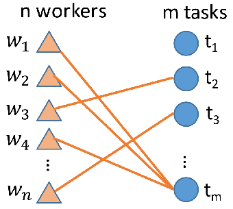
The Time Complexity. We next present the time complexity of the greedy algorithm, MS-SC_Greedy (in Figure 3). Specifically, the time cost of computing valid worker-and-task assignment pairs (line 2) is given by in the worst case, where any of workers can be assigned to any of tasks (i.e., valid worker-and-task pairs). Then, for each round (lines 3-16), we apply pruning methods to pairs, and select the pair with the highest score increase. In the worst case, pairs cannot be pruned, and thus the time complexity of computing score increases for these pairs is given by . Moreover, since each of workers can only be assigned to one spatial task, the number of iterations is at most times. Therefore, the total time complexity of our greedy algorithm can be given by .
V The -Divide-and-Conquer Approach
Although the greedy algorithm incrementally finds one worker-and-task assignment (with the highest score increase) at a time, it may incur the problem of only achieving local optimality. Therefore, in this section, we propose an efficient -divide-and-conquer algorithm (-D&C), which first divides the entire MS-SC problem into subproblems, such that each subproblem involves a smaller subgroup of spatial tasks, and then conquers the subproblems recursively (until the final group size becomes 1). Since different numbers, , of the divided subproblems may incur different time costs, in this paper, we will propose a novel cost-model-based method to estimate the best value to divide the problem.
Specifically, for each subproblem/subgroup (containing tasks), we will tackle the worker-and-task assignment problem via recursion (note: the base case with the group size equal to 1 can be solved by the greedy algorithm [23], which has an approximation ratio of , where is the total number of skills). During the recursive process, we will combine/merge assignment results from subgroups, and obtain the assignment strategy for the merged groups, by resolving the assignment conflict among subgroups. Finally, we can return the task assignment instance set , with respect to the entire worker and tasks sets.
In the sequel, we first discuss how to decompose the MS-SC problem into subproblems in Section V-A. Then, we will illustrate our -divide-and-conquer approach in Section V-B, which utilizes the decomposition and merge (as will be discussed in Section V-C) algorithms. Finally, we will provide a cost model in Section V-D to determine the best number of subproblems during the -D&C process.


V-A MS-SC Problem Decompositions
In this subsection, we discuss how to decompose a MS-SC problem into subproblems. In order to illustrate the decomposition, we first convert our original MS-SC problem into a representation of a bipartite graph.
Bipartite Graph Representation of the MS-SC Problem. Specifically, given a worker set and a spatial task set , we denote each worker/task (i.e., or ) as a vertex in the bipartite graph, where worker and task vertices have distinct vertex types. There exists an edge between a worker vertex and a task vertex , if and only if worker can reach spatial task under the constraints of skills (i.e., ), time (i.e., arrival time is before deadline of arrival), distance (i.e., the traveling distance is below ), and budget (i.e., the traveling cost is below task budget ). We say that the worker-and-task assignment pair is valid, if there is an edge between vertices and in the graph.
As an example in Figure 5(a), we have a worker set , and a spatial task set , which are denoted by two types of vertices (i.e., represented by triangle and circle shapes, respectively) in a bipartite graph. Any edge connects two types of vertices and , if worker can reach the location of task and do tasks with the required skills from . For example, there exists an edge between and , which indicates that worker can move to the location of before the arrival deadline , with the traveling distance under , with the traveling cost below budget , and moreover with some skill(s) in the required skill set of task .
Note that, one or multiple worker vertices (e.g., , , and ) may be connected to the same task vertex (e.g., ). Furthermore, multiple task vertices, say and , may also share some conflicting workers (e.g., or ), where the conflicting worker (or ) can be assigned to either task or task mutual exclusively.
|
Decomposing the MS-SC Problem. Next, we will illustrate how to decompose the MS-SC problem, with respect to task vertices in the bipartite graph. Figure 5 shows an example of decomposing the MS-SC problem (as shown in Figure 5(a)) into 3 subproblems (as depicted in Figure 5(b)), where each subproblem contains a subgroup of one single spatial task (i.e., group size = 1), associated with its connected worker vertices. For example, the first subgroup in Figure 5(b)) contains task vertex , as well as its connecting worker vertices , , and . Different task vertices may have conflicting workers, for example, tasks and share the same (conflicting) worker vertices and .
In a general case, given workers and spatial tasks, we partition the bipartite graph into subgroups, each of which contains spatial tasks, as well as their connecting workers. Figure 6 presents the pseudo code of our MS-SC problem decomposition algorithm, namely MS-SC_Decomposition, which returns MS-SC subproblems (each corresponding to a subgroup with tasks), , after decomposing the original MS-SC problem.
Specifically, we first initialize empty subproblems, , where (lines 1-2). Then, we find out all valid worker-and-task pairs in the crowdsourcing system at timestamp , which can can form a bipartite graph , where valid pairs satisfy the constraints of skills, times, distances, and budgets (line 3).
Next, we want to obtain one subproblem at a time (lines 4-8). In particular, for each round, we retrieve an anchor task and its top- nearest tasks, which form a task set of size (line 5). Here, we choose anchor tasks with a sweeping style, that is, we always choose the task whose longitude is smallest (in the case where multiple tasks have the same longitude, we choose the one with smallest latitude). Then, for each task , we obtain its corresponding vertex in and all of its connecting worker vertices , and add pairs to subproblem (lines 6-8). Finally, we return all the decomposed subproblems .
|
V-B The -D&C Algorithm
In this subsection, we propose an efficient -divide-and-conquer (-D&C) algorithm, namely MS-SC_D&C, which recursively partitions the original MS-SC problem into subproblems, solves each subproblem (via recursion), and merges assignment results of subproblems by resolving the conflicts.
Specifically, in Algorithm MS-SC_D&C, we first estimate the best number of groups, , to partition, with respect to and , which is based on the cost model proposed later in Section V-D (line 2). Then, we will call the MS-SC_Decomposition algorithm (as mentioned in Figure 6) to obtain subproblems (line 3). For each subproblem , if involves more than 1 task, then we can recursively call Algorithm MS-SC_D&C itself, by further dividing the subproblem (lines 5-6). Otherwise, when subproblem contains only one single task, we apply the greedy algorithm of the classical set cover problem for task set and worker set (lines 7-8).
After that, we can obtain an assignment instance set for each subproblem , and merge them into one single worker-and-task assignment instance set , by reconciling the conflict (lines 9-11). In particular, is initially empty (line 1), and each time merged with an assignment set from subproblem (lines 10-11). Due to the confliction among subproblems, we call function MS-SC_Conflict_Reconcile (discussed later in Section V-C) to resolve the confliction issue during the merging process. Finally, we can return the merged assignment instance set (line 12).
V-C Merging Conflict Reconciliation
In this subsection, we introduce the merging conflict reconciliation procedure, which resolves the conflicts while merging assignment results of subproblems (i.e., line 11 of Procedure MS-SC_D&C). Assume that is the current assignment instance set we have merged so far. Given a new subproblem with assignment set , Figure 8 shows the merging algorithm, namely MS-SC_Conflict_Reconcile, which combines two assignment sets and by resolving conflicts.
|
In particular, two distinct tasks from two subproblems may be assigned with the same (conflicting) worker . Since each worker can only be assigned to one spatial task at a time, we thus need to avoid such a scenario when merging assignment instance sets of two subproblems (e.g., and ). Our algorithm in Figure 8 first obtain a set, , of all conflicting workers between and (line 1). Then, each time we greedily solve the conflicts for workers in an non-decreasing order of the traveling cost (i.e., ) in (line 3). Next, in order to resolve the conflicts, we try to replace worker with another worker (or ) in (or ) with the highest score (or ), and compute possible reduction of the assignment score, (or ) (lines 4-7). Note that, here we replace worker with other available workers. If no other workers are available for replacing , we may need to sacrifice task that worker is assigned to. For example, when we cannot find another worker to replace in , the substitute of will be set as an empty worker, which means the assigned task for in will be sacrificed and (as calculated in Equation 2). In the case that , we substitute worker with in (since the replacement of in subproblem leads to lower score reduction); otherwise, we resolve conflicts by replacing with in (lines 8-12). After resolving all conflicts, we merge assignment instance set with (line 13), and return the merged result .
V-D Cost-Model-Based Estimation of the Best Number of Groups
In this subsection, we discuss how to estimate the best number of groups, , such that the total cost of solving the MS-SC problem in -divide-and-conquer approach is minimized. Specifically, the cost of the -divide-and-conquer approach consists of 3 parts: the cost, , of decomposing subproblems, that, , of conquering subproblems recursively, and that, , of merging subproblems by resolving conflicts.
Without loss of generality, as illustrated in Figure 9, during the -divide-and-conquer process, on level , we recursively divide the original MS-SC problem into subproblems, , , …, and , where each subproblem involves spatial tasks.

The Cost, , of Decomposing Subproblems. From Algorithm MS-SC_Decomposition (in Figure 6), we first need to retrieve all valid worker-and-task assignment pairs (line 3), whose cost is . Then, we will divide each problem into subproblems, whose cost is given by on each level. For level , we have tasks in each subproblem . We will further divide it into more subproblems, , and each one will have tasks. To obtain tasks in each subproblem , we first need to find the anchor task, which needs cost, and further retrieve the rest tasks, which needs cost. Moreover, since we will have subproblems on level , the cost of decomposing tasks on level is given by .
Since there are totally levels, the total cost of decomposing the MS-SC problem is given by:
The Cost, , of Recursively Conquering Subproblems. Let function be the total cost of conquering a subproblem which contains spatial tasks. Then, we have the following recursive function:
Assume that is the average degree of task nodes in the bipartite group . Then, the base case of function is the case that , in which we apply the greedy algorithm on just one single task and workers. Thus, by the analysis of the time complexity in Section IV-C, we have:
From the recursive function and its base case, we can obtain the total cost of the recursive invocation on levels from 1 to below:
The Cost, , of Merging Subproblems. Next, we provide the cost, , of merging subproblems by resolving conflicts. Assume that we have workers who could be assigned to more than one spatial task (i.e., conflicting workers). Moreover, each worker node has an average degree in the bipartite graph. During the subproblem merging processing, we can estimate the worst-case cost of resolving conflicts for these workers, and we may resolve conflicts for each worker at most times.
Therefore, the worst-case cost of merging subproblems can be given by:
The Total Cost of the -D&C Approach. The total cost, , of the -D&C algorithm can be given by summing up three costs, , , and . That is, we have
| (4) | |||||
We take the derivation of (given in Eq. (4)) over , and let it be 0. In particular, we have:
| (5) | |||||
We notice that when , is much smaller than 0 but increases quickly when grows. In addition, can only be an integer. Then we can try the integers, (2, 3, 4… ), until is above 0.
VI The Cost-Model-Based Adaptive Algorithm
In this section, we introduce a cost-model-based adaptive approach, which adaptively decides the strategies to apply our proposed greedy and -divide-and-conquer (-D&C) algorithms. The basic idea is as follows. Unlike the -D&C algorithm, we do not divide the MS-SC problem into subproblems recursively until task group sizes become (which can be solved by the greedy algorithm of set cover problems). Instead, based on our proposed cost model, we will partition the problem into subproblems, and adaptively determine when to stop in some partitioning round (i.e., the total cost of solving subproblems with the greedy algorithm is smaller than that of continuing dividing subproblems).
|
VI-A Algorithm of the Cost-Model-Based Adaptive Approach
Figure 10 shows the pseudo-code of our cost-model-based adaptive algorithm, namely MS-SC_Adaptive. Initially, we estimate the cost, , of applying the greedy approach over worker/task sets and (line 2). Similarly, we also estimate the best group size, , and compute the cost, of using the -D&C algorithm (line 3). If it holds that the cost of the greedy algorithm is smaller than that of the -D&C approach (i.e., ), then we will use the greedy algorithm by invoking function MS-SC_Greedy() (due to its lower cost; lines 4-5). Otherwise, we will apply the -D&C algorithm, and further partition the problem into subproblems (lines 6-7). Then, for each subproblem , we recursively call the cost-model-based adaptive algorithm, and retrieve the assignment instance set (line 9). After that, we merge all the assignment instance sets from subproblems by invoking function MS-SC_Conflict_Reconcile() (lines 10-12). Finally, we return the worker-and-task assignment instance set (line 13).
VI-B Cost Model for the Stoping Condition
Next, we discuss how to determine the stopping level, when using our cost-model-based adaptive approach to recursively solve the MS-SC problem. Intuitively, at the current level , we need to estimate the costs, and , of using greedy and -D&C algorithms, respectively, to solve the remaining MS-SC problem. If the greedy algorithm has lower cost, then we will stop the divide-and-conquer, and apply the greedy algorithm for each subproblems.
In the sequel, we discuss how to obtain the formulae of costs and .
The Cost, , of the Greedy Algorithm. Given a set, , of workers and a set, , of tasks, the cost, , of our greedy approach (as given in Figure 3) has been discussed in Section IV-C.
In the bipartite graph of valid worker-and-task pairs, denote the average degree of workers as , and that of tasks as . In Figure 3, the computation of valid worker-and-task pairs in line 2 needs cost. Since there are at most iterations, for each round (lines 3-16), we apply two worker-pruning methods to at most pairs, and select pairs with the highest score increases, which need cost in total. For the cost of task-pruning, there are totally rounds (lines 3-16; i.e., removing one out of workers in each round in line 16). In each round, there are at most out of tasks (line 5) that may be potentially pruned by Lemma 4 (line10). To check each of tasks, we need cost. Therefore, the total cost of task-pruning is given by . If we cannot prune a task that was assigned with a worker in the last round (lines 3-16), then we need to update score increases of workers for that task. Each task will be assigned with workers for times. Thus, the total update cost for one task is given by (line 12). Therefore, can be given by:
| (6) | |||||
where parameter is a constant factor, which can be inferred from cost statistics of the greedy algorithm.
The Cost, , of the -D&C Algorithm. Assume that the current -divide-and-conquer level is . We can modify the cost analysis in Section V-D, by considering the cost, , of the remaining divide-and-conquer levels. Specifically, we have the cost, , of the decomposition algorithm, that is:
Moreover, when the current level is , the cost of conquering the remaining subproblems is given by:
Finally, the cost of merging subproblems is given by .
As a result, the total cost, , of solving the MS-SC problem with our -D&C approach for the remaining partitioning levels (from level to ) can be given by:
where parameter is a constant factor, which can be inferred from time cost statistics of the -D&C algorithm.
This way, we compare with (as mentioned in line 4 of MS-SC_Adaptive Algorithm). If is smaller than , we stop at the current level , and apply the greedy algorithm to tackle the MS-SC problem directly; otherwise, we keep dividing the original MS-SC problem into subproblems (i.e., -D&C).
VII Experimental Study
VII-A Experimental Methodology
Data Sets. We use both real and synthetic data to test our proposed MS-SC approaches. Specifically, for real data, we use Meetup data set from [18], which was crawled from meetup.com between Oct. 2011 and Jan. 2012. There are 5,153,886 users, 5,183,840 events, and 97,587 groups in Meetup, where each user is associated with a location and a set of tags, each group is associated with a set of tags, and each event is associated with a location and a group who created the event. For an event, we use the tags of the group who creates the event as its tags. To conduct the experiments on our approaches, we use the locations and tags of users in Meetup to initialize the locations and the practiced skills of workers in our MS-SC problem. In addition, we utilize the locations and tags of events to initialize the locations and the required skills of tasks in our experiments. Since workers are unlikely to move between two distant cities to conduct one spatial task, and the constraints of time (i.e., ), budget (i.e., ) and distance (i.e., ) also prevent workers from moving too far, we only consider those user-and-event pairs located in the same city. Specifically, we select one famous and popular city, Hong Kong, and extract Meetup records from the area of Hong Kong (with latitude from to and longitude from to ), in which we obtain 1,282 tasks and 3,525 workers.
For synthetic data, we generate locations of workers and tasks in a 2D data space , following either Uniform (UNIFORM) or Skewed (SKEWED) distribution. For Uniform distribution, we uniformly generate the locations of tasks/workers in the 2D data space. Similarly, we also generate tasks/workers with the Skewed distribution by locating 90% of them into a Gaussian cluster (centered at (0.5, 0.5) with variance = ), and distribute the rest workers/tasks uniformly. Then, for skills of each worker, we randomly associate one user in Meetup data set to this worker, and use tags of the user as his/her skills in our MS-SC system. For the required skills of each task, we randomly select an event, and use its tags as the required skills of the task.
For both real and synthetic data sets, we simulate the velocity of each worker with Gaussian distribution within range , for . For the unit price, , w.r.t. the traveling distance of each worker, we generate it following the Uniform distribution within the range . Furthermore, we produce the maximum moving distance of each worker, following the Uniform distribution within the range (for ). For temporal constraints of tasks, we also generate the arrival deadlines of tasks, , within range with Gaussian distribution. Finally, we set the budgets of tasks with Gaussian distribution within the range . Here, for Gaussian distributions, we linearly map data samples within of a Gaussian distribution to the target ranges.
MS-SC Approaches and Measures. We conduct experiments to compare our three approaches, GREEDY, -D&C and ADAPTIVE, with a random method, namely RANDOM, which randomly assigns workers to tasks.
In particular, GREEDY selects a “best” worker-and-task assignment with the highest score increase each time, which is a local optimal approach. The -D&C algorithm keeps dividing the problem into subproblems on each level, until finally the number of tasks in each subproblem is 1 (which can be solved by the greedy algorithm on each one-task subproblem). Here, the parameter can be estimated by a cost model to minimize the computing cost. The cost-model-base adaptive algorithm (ADAPTIVE) makes the trade-off between GREEDY and -D&C, in terms of efficiency and accuracy, which adaptively decides the stopping level of the divide-and-conquer. To evaluate our three proposed approaches, we need to compare the results with ground truth. However, as proved in Section II-D, the MS-SC problem is NP-hard, and thus infeasible to calculate the real optimal result as the ground truth. Alternatively, we will compare the effectiveness of our three approaches with that of a random (RANDOM) method, which randomly chooses a task then randomly assigns worker to the task. For each MS-SC instance, we run RANDOM for 10 times, and report the result with the highest score.
Table IV depicts our experimental settings, where the default values of parameters are in bold font. In each set of experiments, we vary one parameter, while setting other parameters to their default values. For each experiment, we report the running time and the assignment score of our tested approaches. All our experiments were run on an Intel Xeon X5675 CPU @3.07 GHZ with 32 GB RAM in Java.
| Parameters | Values |
|---|---|
| the number of tasks | 1K, 2K, 5K, 8K, 10K |
| the number of workers | 1K, 2K, 5K, 8K, 10K |
| the task budget range | [1, 5], [5, 10], [10, 15], [15, 20], [20, 25] |
| the velocity range | [0.1, 0.2], [0.2, 0.3], [0.3, 0.4], [0.4, 0.5] |
| the unit price w.r.t. distance | [10, 20], [20, 30], [30, 40], [40, 50] |
| the moving distance range | [0.1, 0.2], [0.2, 0.3], [0.3, 0.4], [0.4, 0.5] |
| the expiration time range | [0.25, 0.5], [0.5, 1], [1, 2], [2, 3], [3, 4] |
VII-B Experiments on Real Data
In this subsection, we show the effects of the range of task budgets , the range of workers’ velocities , and the range of unit prices w.r.t. distance .
Effect of the Range of Task Budgets . Figure 11 illustrates the experimental results on different ranges, , of task budgets from to . In Figure 11(a), the assignment scores of all the four approaches increase, when the value range of task budgets gets larger. When the average budgets of tasks increase, the flexible budget of each task will also increase. -D&C and ADAPTIVE can achieve higher score than GREEDY. In contrast, RANDOM has the lowest score, which shows that our proposed three approaches are more effective. As shown in Figure 11(b), the running times of our three approaches increase, when the range of task budgets becomes larger. The reason is that, when increases, each task has more valid workers, which thus leads to higher complexity of the MS-SC problem and the increase of the running time. The RANDOM approach is the fastest (however, with the lowest assignment score), since it does not even need to find local optimal assignment. The ADAPTIVE algorithm achieves much lower running time than -D&C (a bit higher time cost than GREEDY), but has comparable score with -D&C (much higher score than GREEDY), which shows the good performance of ADAPTIVE, compared with GREEDY and -D&C.


Effect of the Workers’ Velocity Range . Figure 12 reports the effect of the range of velocities, , of workers over real data. As shown in Figure 12(a), when the range of velocities increases from to , the scores of all the approaches first increase; then, they stop growing for the velocity range varying from [0.2, 0.3] to [0.4, 0.5]. The reason is that, at the beginning, with the increase of velocities, workers can reach more tasks before their arrival deadlines. Nevertheless, workers are also constrained by their maximum moving distances, which prevents them from reaching more tasks. ADAPTIVE can achieve a bit higher scores than -D&C, and much better assignment scores than GREEDY.
In Figure 12(b), when the range of velocity increases, the running times of our tested approaches also increase, due to the cost of more valid worker-and-task pairs to be handled. Similar to previous results, RANDOM is the fastest, and -D&C is the slowest. ADAPTIVE requires about 0.5-1.5 seconds, and has lower time cost than -D&C, which shows the efficiency of our proposed approaches.


Effect of the Range of Unit Prices w.r.t. Traveling Distance . In Figure 13(a), when the unit prices w.r.t. traveling distance increase, the scores of all the approaches decrease. The reason is that, when the range of unit prices increases, we need to pay more wages containing the traveling costs of workers (to do spatial tasks), which in turn decreases the flexible budget of each task. However, ADAPTIVE can still achieve the highest score among all four approaches; scores of -D&C are close to the scores of ADAPTIVE and higher than GREEDY.
In Figure 13(b), when the range of unit prices, , of the traveling cost increases, the number of valid worker-and-task pairs decreases, and thus the running time of all the approaches also decreases. Our ADAPTIVE algorithm is faster than -D&C, and slower than GREEDY.


In addition, we also tested the effects of the range, , of maximum moving distances for workers, and the expiration time range, , of tasks over the real data set, Meetup. Due to space limitations, please refer to experimental results with respect to other parameters (e.g., and ) in Appendix F.
From experimental results on the real data above, ADAPTIVE can achieve higher scores than Greedy and -D&C, and it is faster than -D&C and slower than GREEDY. Although -D&C can achieve good scores close to ADAPTIVE, it is the slowest among all the 4 approaches.
VII-C Experiments on Synthetic Data
In this subsection, we test the effectiveness and robustness of our three MS-SC approaches, GREEDY, -D&C, and ADAPTIVE, compared with RANDOM, by varying parameters (e.g., the number of tasks and the number of workers ) on synthetic data sets. Due to space limitations, we present the experimental results for tasks/workers with Uniform distributions. For similar results with tasks/workers following skewed distributions, please refer to Appendix G.
Effect of the Number of Tasks . Figure 14 illustrates the effect of the number, , of spatial tasks, by varying from to , over synthetic data sets, where other parameters are set to default values. For assignment scores in Figure 14(a), -D&C obtains results with the highest scores among all the four approaches. ADAPTIVE performs similar to -D&C, and achieves good results similar to -D&C. GREEDY is not as good as -D&C and ADAPTIVE, but is still much better than RANDOM. When the number, , of spatial tasks becomes larger, all our approaches can achieve higher scores.
In Figure 14(b), when increases, the running time also increases. This is because, we need to deal with more worker-and-task assignment pairs for large . The ADAPTIVE algorithm is slower than GREEDY, and faster than -D&C. In addition, we find that the running time of GREEDY performs, with the same trend as that estimated in our cost model (as given in Eq. (6)).


Effect of the Number of Workers . Figure 15 shows the experimental results with different numbers of workers, , from to over synthetic data, where other parameters are set to their default values. Similar to previous results about the effect of , in Figure 15(a), our proposed three approaches can obtain good results with high assignment scores, compared with RANDOM. Moreover, when the number, , of workers increases, the scores of all our approaches also increase. The reason is that, when increases, we have more potential workers, who can be assigned to nearby tasks, which may lead to even larger scores.
In Figure 15(b), the running time of our approaches increases, with the increase of the number of workers . This is due to higher cost to process more workers (i.e., larger ). Similarly, ADAPTIVE has higher time cost than GREEDY, and lower time cost than -D&C.


In summary, over synthetic data sets, our ADAPTIVE algorithm trades the accuracy for efficiency, and thus has the trade-off of scores/times between GREEDY and -D&C.
VIII Related Work
Recently, with the popularity of GPS-equipped smart devices and wireless networks (e.g., Wi-Fi and 4G), the spatial crowdsourcing [12, 16] that performs location-based tasks has emerged and become increasingly important in both academia and industry. In this section, we review the related work on spatial crowdsourcing, as well as the set cover problem (and its variants).
Spatial Crowdsourcing. Prior works on crowdsourcing [5, 7] usually studied crowdsourcing problems, which treat the location information as a parameter and distribute tasks to workers. In these problems, workers are not required to accomplish tasks on sites.
In contrast, the spatial crowdsourcing platform [16] requires workers to physically move to some specific locations of tasks, and perform the requested services, such as taking photos/videos, waiting in line at shopping malls, and decorating a room. As an example, some previous works [11, 14] studied the small-scale or specified campaigns benefiting from participatory sensing techniques, which utilize smart devices (equipped by workers) to sense/collect data for real applications.
Kazemi and Shahabi [16] classified the spatial crowdsourcing systems from two perspectives: people’s motivation and publishing models. From the perspective of people’s motivation, the spatial crowdsourcing can be categorized into two groups: reward-based, in which workers can receive rewards according to the services they supplied, and self-incentivised, in which workers conduct tasks voluntarily. In our work, we study our MS-SC problem based on the reward-based model, where workers are paid for doing tasks. However, with a different goal, our MS-SC problem targets at assigning workers to tasks by using our proposed algorithms, such that the required skills of tasks can be covered, and the total reward budget (i.e., flexible budget in Eq. (2)) can be maximized. Note that, we can embed incentive mechanisms from existing works [20, 24] into our MS-SC framework to distribute rewards (flexible budgets) among workers, which is however not the focus of our problem.
According to the publishing modes of spatial tasks, the spatial crowdsourcing can be also classified into two categories: worker selected tasks (WST) and server assigned tasks (SAT) [16]. In particular, for the WST mode, spatial tasks are broadcast to all workers, and workers can select any tasks by themselves. In contrast, for the SAT mode, the spatial crowdsourcing server will directly assign tasks to workers, based on location information of tasks/workers.
Some prior works [5, 12] on the WST mode allowed workers to select available tasks, based on their personal preferences. However, for the SAT mode, previous works focused on assigning available workers to tasks in the system, such that the number of assigned tasks on the server side [16], the number of worker’s self-selected tasks on the client side [12], or the reliability-and-diversity score of assignments [10] is maximized. For example, Peng et al. [10] aims to obtain a worker-and-task assignment strategy such that the assignment score (w.r.t. spatial/temporal diversity and reliability of tasks) is maximized.
In contrast, our MS-SC problem has a different, yet more general, goal, which maximizes the total assignment score (i.e., flexible budget, given by the total budget of the completed tasks minus the total traveling cost of workers). Most importantly, in our MS-SC problem, we need to consider several constraints, such as skill-covering, budget, time, and distance constraints. That is, the required skill sets of spatial tasks should be fully covered by skills of those assigned workers, which is NP-hard and intractable. Thus, previous techniques [10, 12, 16] on different spatial crowdsourcing problems cannot be directly applied to our MS-SC problem.
Some research communities studied the theory of SAT problems and developed some SAT (Satisfiability) solvers. However, standard SAT solvers can only solve decision problems (i.e., NP-complete problems), but not optimization problems (i.e., NP-hard problems, like our MS-SC problem). Thus, we need to design specific heuristic algorithms for tackling the MS-SC problem.
Moreover, some previous works [19, 22] utilized differential privacy techniques [13] to protect the location information, which is used to do the assignment, but may release some sensitive location/trajectory data (leading to malicious attacks). Nevertheless, this privacy issue is out of the scope of this paper.
Set Cover Problem. As mentioned in Lemma 1, the set cover problem (SCP) is a classical NP-hard problem, which targets at choosing a set of subsets to cover a universe set, such that the number of the selected subsets is minimized. SCP is actually a special case of our MS-SC problem, in which there exists only one spatial task. However, in most situations, we have more than one spatial task in the spatial crowdsourcing system, which is more complex, and thus more challenging, to tackle.
A direct variant of SCP is the weighted set cover problem, which associates each subset with a weight. The well-known greedy algorithm [23] can achieve an approximation ratio of here , where is the size of the universe set. Other SCP variants, such as the set multicover problem (SMC) and multiset multicover problem (MSMC), focused on covering each element of the universe set for at least specified times using sets (in SMC, each element in subsets has just one copy) or multisets (in MSMC, each element in subsets has a specified number of copies). Sun and Li [21] studied set cover games problem, which covers multiple sets. However, they focused on designing a good mechanism to enable each single task to obtain a local optimal result. In contrast, our work aims to obtain a global optimal solution to maximize the score of assignment.
Different from SCP and its variants that cover only one universe set, our MS-SC problem is targeting to cover multiple sets, such that the assignment score is maximized. Furthermore, our MS-SC problem is also constrained by budget, time, and distance, which is much more challenging than SCP. To the best of our knowledge, no prior works on SCP (and its variants) have studied the MS-SC problem, and existing techniques cannot be used directly to tackle the MS-SC problem.
IX Conclusion
In this paper, we propose the problem of the multi-skill oriented spatial crowdsourcing (MS-SC), which assigns the time-constrained and multi-skill-required spatial tasks with dynamically moving workers, such that the required skills of tasks can be covered by skills of workers and the assignment score is maximized. We prove that the processing of the MS-SC problem is NP-hard, and thus we propose three approximation approaches (i.e., greedy, -D&C, and cost-model-based adaptive algorithms), which can efficiently retrieve MS-SC answers. Extensive experiments have shown the efficiency and effectiveness of our proposed MS-SC approaches on both real and synthetic data sets.
References
- [1] Foursquare. https://foursquare.com.
- [2] Google street view. https://www.google.com/maps/views/streetview.
- [3] Taskrabbit. https://www.taskrabbit.com.
- [4] Waze. https://www.waze.com.
- [5] F. Alt, A. S. Shirazi, A. Schmidt, U. Kramer, and Z. Nawaz. Location-based crowdsourcing: extending crowdsourcing to the real world. In NordiCHI 2010: Extending Boundaries, 2010.
- [6] A. Belussi and C. Faloutsos. Self-spacial join selectivity estimation using fractal concepts. TOIS, 16(2):161–201, 1998.
- [7] M. F. Bulut, Y. S. Yilmaz, and M. Demirbas. Crowdsourcing location-based queries. In PERCOM Workshops 2011, pages 513–518.
- [8] Z. Chen, R. Fu, Z. Zhao, Z. Liu, L. Xia, L. Chen, P. Cheng, C. C. Cao, and Y. Tong. gmission: A general spatial crowdsourcing platform. VLDB 2014, 7(13).
- [9] P. Cheng, X. Lian, L. Chen, J. Han, and J. Zhao. Task assignment on multi-skill oriented spatial crowdsourcing (technical report). http://arxiv.org/abs/1510.03149.
- [10] P. Cheng, X. Lian, Z. Chen, R. Fu, L. Chen, J. Han, and J. Zhao. Reliable diversity-based spatial crowdsourcing by moving workers. VLDB 2015, 8(10).
- [11] C. Cornelius, A. Kapadia, D. Kotz, D. Peebles, and M. Shin. Anonysense: privacy-aware people-centric sensing. MobiSys 2008.
- [12] D. Deng, C. Shahabi, and U. Demiryurek. Maximizing the number of worker’s self-selected tasks in spatial crowdsourcing. In SIGSPATIAL GIS 2013, pages 314–323.
- [13] C. Dwork. Differential privacy: A survey of results. In Theory and applications of models of computation, pages 1–19. Springer, 2008.
- [14] S. S. Kanhere. Participatory sensing: Crowdsourcing data from mobile smartphones in urban spaces. In MDM 2011, volume 2. IEEE.
- [15] R. M. Karp. Reducibility among combinatorial problems. Springer, 1972.
- [16] L. Kazemi and C. Shahabi. Geocrowd: enabling query answering with spatial crowdsourcing. In SIGSPATIAL GIS 2012, pages 189–198.
- [17] S. H. Kim, Y. Lu, G. Constantinou, C. Shahabi, G. Wang, and R. Zimmermann. Mediaq: mobile multimedia management system. In MMSys 2014, pages 224–235. ACM.
- [18] X. Liu, Q. He, Y. Tian, W.-C. Lee, J. McPherson, and J. Han. Event-based social networks: linking the online and offline social worlds. In Proceedings of ACM SIGKDD 2012, pages 1032–1040. ACM, 2012.
- [19] L. Pournajaf, L. Xiong, V. Sunderam, and S. Goryczka. Spatial task assignment for crowd sensing with cloaked locations. In Mobile Data Management (MDM), volume 1, pages 73–82. IEEE, 2014.
- [20] J. P. Rula, V. Navda, F. E. Bustamante, R. Bhagwan, and S. Guha. No one-size fits all: Towards a principled approach for incentives in mobile crowdsourcing. In HotMobile 2014. ACM.
- [21] Z. Sun, X.-Y. Li, W. Wang, and X. Chu. Mechanism design for set cover games when elements are agents. In Algorithmic Applications in Management, pages 360–369. Springer, 2005.
- [22] H. To, G. Ghinita, and C. Shahabi. A framework for protecting worker location privacy in spatial crowdsourcing. VLDB 2014, 7(10):919–930.
- [23] V. V. Vazirani. Approximation algorithms. Springer Science & Business Media, 2013.
- [24] D. Yang, G. Xue, X. Fang, and J. Tang. Crowdsourcing to smartphones: incentive mechanism design for mobile phone sensing. MobiCom 2012.
-A Proof of Lemma 1
Proof:
We prove the lemma by a reduction from the set cover problem (SCP). A set cover problem can be described as follows: Given a universe set and m subsets . For each subset , it is associated with a cost . The set cover problem is to find a set that minimizes , such that .
For a given set cover problem, we can transform it to an instance of MS-SC as follows: at timestamp , we give only one task with required skills set and , whose budget value, , is big enough to hire workers to satisfy the required skills. In addition, the arrival deadline of the task is late enough for any worker to arrive in time. For workers, each worker has a skills set , such that , and a cost . In addition, the maximum moving distance is larger than . Then, for this MS-SC instance, we want to select workers to support task that maximizes the score, and .
The answer of this MS-SC is:
As is a constant, to maximize the score is same as to minimize the total cost, , of the assigned workers, which is identical to . Given this mapping it is easy to show that the set cover problem instance can be solved if and only if the transformed MS-SC problem can be solved.
This way, we can reduce SCP to the MS-SC problem. Since SCP is known to be NP-hard [23], MS-SC is also NP-hard, which completes our proof. ∎
-B Proof of Lemma 2
Proof:
We want to prove that, if worker is assigned to task , then any skill can be also covered by worker . From the lemma assumption, since worker is dominated by , we have and . Thus, from the condition that , we have . Moreover, since , from Eq. (3), we have . Therefore, worker is not better than worker , in terms of the score increase. Hence, we can safely prune the worker-and-task pair . ∎
-C Proof of Lemma 3
Proof:
From Definition 4, we have the budget constraint that . From the lemma assumption, if it holds that , then we have , which violates the constraint that the total traveling cost should not exceed the maximum budget . Thus, we should not assign worker to task .
Due to the non-increasing property of the remaining budget , for the rest of assignment rounds, we still cannot assign worker to (since the task cannot afford the traveling cost of the worker ). Hence, we can safely prune worker . ∎
-D Proof of Lemma 4
Proof:
Since the traveling cost, , of worker is greater than the remaining budget, , according to Lemma 3, worker should not be assigned to task .
Therefore, we only need to prove that, for any set of the remaining unassigned workers who can cover the required skill set , their total traveling cost is always greater than the remaining budget .
Without loss of generality, assume that we have a subset, , of unassigned workers, , in that can be assigned to task , and cover the skill set (note: if such a subset does not exist, then task cannot be fully covered by workers’ skills and can be safely pruned). Then, we have the relationship of skill sets between worker (with the highest value) and workers below:
Alternative, we can derive the relationship of their set sizes, that is:
| (7) | |||||
On the other hand, according to Eq. (3) and our lemma assumption (i.e., worker has the largest value of ), for any worker , we have the following relationship between and :
As a result, the total traveling cost for all has the property below:
| (8) |
| (9) |
Since it holds that by the lemma assumption, we thus have:
| (10) |
which exactly indicates that any subset, , of those unassigned workers has the total traveling cost exceeding the remaining budget. Hence, we can safely prune task , and the lemma holds. ∎
-E MS-SC Grid Index
In order to facilitate the processing of the MS-SC problem, we present an efficient cost-model-based indexing mechanism, which can maintain workers and tasks and help the retrieval of MS-SC answers.
Index Structure. We first introduce the index structure, namely MS-SC-Grid, for the MS-SC system. In particular, we divide a 2-dimensional data space, , into square cells with side length , where . Similar to the cost model of the grid index in [10], by utilizing the power law [6] for the correlation fractal dimension of the tasks and workers in the 2D data space, we can construct a cost model of updating the grid index after insert or delete a worker with respect to the side length . Then we can estimate the best value for to minimize the update cost.
Below, we will illustrate the content of each cell, , in the grid index, which includes worker/task lists, statistics of workers/tasks, and a cell list.
Worker and Task Lists in Cells. Within the grid index, each cell, , has a unique ID, , and is associated with two lists, which store sets of tasks and workers, respectively, that reside in the cell. In the worker list, we maintain records, in the form of sextuple:
where is the worker ID, , , , and represent the location, constant related to the traveling cost of the distance, maximum moving distance, and velocity of the worker, respectively, and is a set of skills that the worker has.
In the task list, we keep records in the form:
where is the task ID, is the location of the task, denotes the arrival deadline of the task, represents the budget of the task, and is the set of skills required by the task.
Statistics/Aggregates in Cells. For each cell , we maintain statistics/aggregates for workers and tasks in it, including:
- •
the minimum constant for the traveling cost ;
- •
the largest maximum moving distance ;
- •
the maximum velocity, , for all workers in the cell;
- •
the latest arrival deadline ;
- •
the maximum budget, , for all tasks in the cell;
- •
the union, , of sets of workers’ skills; and
- •
the union, , of sets of the required skills by tasks in the cell.
Synopses for Skill Sets. In order to time- and space-efficiently organize/manipulate the sets of skills for workers and tasks (i.e., and above, respectively), an alternative is to maintain two bitmap synopses, and , in which each bit corresponds to a skill. That is, for any skill in the skill set (or ), its corresponding bit in bitmap (or ) is set to “1”; the remaining bits in (or ) are set to “0”. This way, we can apply bit operations (e.g., bit-AND or bit-OR) between any two synopses, and check the relationship (e.g., containment or intersection) between their corresponding skill sets.
Cell List. Furthermore, each cell is also associated with a cell list, , which contains all the cell IDs that can be reachable to at least one worker in cell .
Pruning Strategy on the Cell Level. When calculate the valid worker-and-task pairs for worker in our approaches, we can use the grid index to accelerate the searching time by just checking the cells in the of the cell and the cell itself, where worker locates in cell . However, we do not need to check all the tasks in the cells in . We propose 4 pruning strategies to further reduce the search space.
Assuming we are searching the valid worker-and-task pairs for worker located in cell , we now show how to prune a cell in before further checking all the tasks in . We first calculate the minimum distance between the location of worker and any points in . Then we have 4 pruning strategies.
- •
If , all the tasks in are out of the working range of worker , that is, worker will not accept any task in ;
- •
If , worker cannot arrive any task in before the arrival deadline of that task;
- •
If , no task in can afford the traveling cost of worker ;
- •
If , worker cannot support any skills of any task in .
If any one strategy is met, we can safely prune cell . After pruning those unreachable or unsupportable cells, we further check the rest cells one by one to construct the valid worker-and-task pairs for worker .
Dynamic Index Maintenance. Since workers/tasks can join and leave the spatial crowdsourcing system, our grid index should be efficient for handling worker/task updates. Specifically, for each incoming/expired worker/task, we update contents of cells that workers/tasks fall into, as well as the cell list. Due to space limitations, we will not discuss insertion/detetion of workers/tasks in detail.

Figure 16 presents the index retrieval time (i.e., the time cost of retrieving valid worker-and-task pairs) over UNIFORM data, where and varies from 500 to 10K. The MS-SC grid index can reduce the time of obtaining worker-and-task pairs dramatically (up to 79%), compared with the running time of directly enumerating and checking all possible worker-and-task pairs.
-F Effects of Moving Distance and Expiration Times
In this subsection, we show the effects of the range of maximum moving distances of workers, , and the range of the expiration time of tasks, .
Effect of Range of Workers’ Maximum Moving Distances . Figure 17 shows the effect of the range of worker’s maximum moving distances on the scores of assignments and the running times, where we vary the range of from to . In Figure 17(a), all the 3 approaches can achieve good scores of assignment. They still has a comparison sequence on the score of the results: the score of the results obtained by ADAPTIVE is highest among other approaches in our experiments. Then, -D&C can also get a higher score of assignment than GREEDY. Similar to the discuss of the effect of the velocities of workers, the increase of enlarges the access range of workers at the beginning. However, when the constraint of is relaxed, the constraints from other parameters prevent the scores keeping growing.
For the running times, Adaptive is faster than -D&C, but slower than Greedy. Random runs fastest, however, least effectively.


Effect of Range of Expiration Times of Tasks . Figure 18 shows the effect of the range of tasks’ expiration times on the scores of assignments and the running times, where we vary the range of from to . In Figure 18(a), all the 3 approaches can achieve good scores of assignment. ADAPTIVE still obtains highest scores compared with other approaches, and -D&C is better than Greedy in scores, however not as good as Adaptive. Random just can receive lower scores. Similar to the discuss of the effect of the velocities of workers, the increase of enlarges the access range of workers at the beginning. However, when the constraint of is relaxed, the constraints from other parameters prevent the scores from keeping growing.


For the running times, all the approaches use more time when the range of expiration times increases, which is because workers can arrive at more tasks before their arrival deadlines leading to the problem space increases. Comparatively, Adaptive is faster than -D&C, but slower than Greedy. Random runs fastest, however least effectively.
-G Effect of Number of Task and Workers (SKEWED)
Effect of Number of Tasks . Figure 19 illustrates the effect of the number of tasks, when changing from 1K to 10K, and the distribution of the location of workers and tasks are SKEWED. For the scores of assignments in Figure 19(a), -D&C obtains results with highest scores. ADAPTIVE performs similar to -D&C and also achieves good results. GREEDY is not as good as -D&C and ADAPTIVE, but still much better than RANDOM. All the approaches can obtain a higher score when the number of tasks become larger. In Figure 19(b), the running times increase when the number of tasks increase, because the problem space increases. The Adaptive is slower than Greedy and faster than -D&C.


Effect of Number of Workers . Figure 20 shows the experimental results when the number of workers, , changing from 1K to 10K, and the distribution of the location of workers and tasks are SKEWED. Similar to the results in previous discussion of the effect of , our three approaches can obtain good results with high scores of assignment. In addition, the scores of all the approaches increase when the number of workers increases. The reason is that, when the number of workers increases, we have more workers, who are close to tasks and cost less, to select, which leads to the score increases. In Figure 20(b), the running times increase when the number of workers increases, because the space of problem increases when there are more workers. The speed of Adaptive is higher than -D&C and lower than Greedy.

