Error estimates of finite element method for semi-linear stochastic strongly damped wave equation
Abstract
In this paper, we consider a semi-linear stochastic strongly damped wave equation driven by additive Gaussian noise. Following a semigroup framework, we establish existence, uniqueness and space-time regularity of a mild solution to such equation. Unlike the usual stochastic wave equation without damping, the underlying problem with space-time white noise () allows for a mild solution with a positive order of regularity in multiple spatial dimensions. Further, we analyze a spatio-temporal discretization of the problem, performed by a standard finite element method in space and a well-known linear implicit Euler scheme in time. The analysis of the approximation error forces us to significantly enrich existing error estimates of semidiscrete and fully discrete finite element methods for the corresponding linear deterministic equation. The main results show optimal convergence rates in the sense that the orders of convergence in space and in time coincide with the orders of the spatial and temporal regularity of the mild solution, respectively. Numerical examples are finally included to confirm our theoretical findings.
Key words. strongly damped wave equation, Wiener process, finite element method, linear implicit Euler scheme, strong approximation
1 Introduction
The present work is concerned with the following semi-linear stochastic evolution equation subject to additive noise, described by
where , , is a bounded, convex and polynomial domain with a boundary and is a fixed positive constant. Let be a linear second-order elliptic operator with smooth coefficients and being uniformly positive definite. Let be a (possibly cylindrical) -Wiener process on , defined on a stochastic basis with respect to a normal filtration and let be -measurable random variables.
The considered problem (1) is referred to as stochastic strongly damped wave equation (SSDWE for short) thereafter. The deterministic counterpart of (1) finds many applications in viscoelastic theory [7, 15, 16], and its linear version has been numerically studied by [14, 21], where a finite element method is used for spatial discretization and rational approximations for analytic semigroup. Particularly when , the problem (1) reduces to a stochastic wave equation (SWE) without damping, numerical approximations of which have been recently studied by many authors [2, 3, 4, 5, 8, 11, 12, 22, 19, 24, 23, 9, 10, 17, 18]. In contrast to the SWE case (), the stochastic strongly damped wave equations () are much less well-understood, from both theoretical and numerical point of view. In [6, Example 6.25], a linear version of SSDWE with multiplicative noise was examined and its unique mild solution was verified. To the best of our knowledge, regularity analysis and numerical treatment of such stochastic problem are both missing in the literature. This article aims to fill the gap and investigate the regularity properties and strong approximations of SSDWE like (1).
Reformulating (1) as a Cauchy problem of first order in a Hilbert space, we follow the semigroup framework as in [6] to show existence, uniqueness and space-time regularity of a mild solution to (1). Under some standard assumptions (Assumptions 2.1-2.3), it is revealed that (see Theorem 2.4), the unique mild solution exhibits the Sobolev and Hölder regularity properties as follows,
| (1.4) |
where, as specified later, , and the parameter satisfying quantifies the spatial correlation of the noise process (Assumption 2.2). If and , then
| (1.5) |
In order to achieve (1.4)-(1.5), we exploit further spatial and temporal regularity properties of the linear deterministic equation (Lemmas 2.8-2.9), based on an existing spatial regularity result (Lemma 2.7) in [14]. From (1.4)-(1.5), it is easy to realize that, the mild solution of (1) () enjoys higher spatial and temporal regularity than that of the usual stochastic wave equation (), which only admits a mild solution taking values in and satisfying under the same assumptions [2, 23]. This benefits from smoothing effect of the analytic semigroup generated by the dominant linear operator . In particular, different from both the stochastic heat equation and the stochastic wave equation, the strongly damped problem driven by space-time white noise () allows for a mild solution with a positive order of regularity in multiple spatial dimensions (). For example, the space-time white noise case when admits a mild solution for any (consult Remark 2.5 for more details).
As the second contribution of this article, we analyze the mean-square approximation errors caused by finite element spatial semi-discretization and space-time full-discretization of (1). More precisely, we measure the discrepancy between the mild solution and the finite element spatial approximation as follows (Theorem 4.1):
| (1.6) |
where the parameter restricted to , similarly as before, characterizes the spatial correlation of the Wiener process. By a combination of the finite element method (FEM) together with a linear implicit Euler-Maruyama time-stepping scheme, we also investigate a spatio-temporal discretization of (1). As stated in Theorem 4.3, the corresponding strong approximation error satisfies
| (1.7) |
Here and are, respectively, full-discrete approximations of and . Comparing the convergence results (1.6)-(1.7) with the regularity results (1.4)-(1.5), one can readily observe that, the convergence rates obtained here are optimal in the sense that the rates of convergence in space and in time coincide with the orders of the spatial and temporal regularity of the mild solution, respectively. This essentially differs from the SWE setting (), where the strong rates of the FEM coupled with the linear implicit Euler scheme are lower than orders of the spatial and temporal regularity of the mild solution (e.g., [13, 12]).
Before proving (1.6)-(1.7), we formulate in section 3 a rich variety of error estimates for the finite element semi-discretization and full-discretization of the corresponding deterministic linear problem. Some of such error estimates can be straightforwardly derived from existing ones in [14] by ingenious modifications or by interpolation arguments (Theorems 3.1, 3.4). Nevertheless, we must stress that, error estimates available in [14] are far from enough for the purpose of our error analysis. For instance, as one can see later, two completely new error estimates of integral form such as (3.27) and (3.86) are indispensable in the error analysis and their proofs turn out to be quite involved. To show the error estimate (3.27) for the semi-discretization, we rely on energy arguments and interpolation theory (see the proof of Theorem 3.3). The proof of (3.86) for the full-discretization is, however, more complicated and more technical. In addition to energy arguments and interpolation theory, we need some further integral versions of regularity results of the linear deterministic problem as presented in Lemma 3.5. Armed with these error estimates, we are then able to establish (1.6)-(1.7) for the stochastic problem (see section 4 for the details).
The outline of this paper is as follows. In the next section, some preliminaries are collected and the well-posedness of the considered problem is elaborated. Section 3 is devoted to error estimates of semi-discrete and full-discrete finite element method for the corresponding deterministic linear problem. The main convergence results for the stochastic problem are presented in section 4. Numerical experiments are finally performed in section 5 to confirm the theoretical results.
2 The stochastic strongly damped wave equation
Let and be two separable -Hilbert spaces and by we denote the Banach space of all linear bounded operators from into and by the Hilbert space of all Hilbert-Schmidt operators from into . When , we write and for ease of notation. Also, we denote the space of the Hilbert-Schmidt operators from to by and the corresponding norm is given by It is well-known that Additionally, we denote with the domain and define
It is clear that , and . Now we reformulate the stochastic equation (1) as the following abstract form
where , and
Here generates an analytic semigroup in , (see [14, Lemma 2.1]). For the purpose of the existence, uniqueness and regularity of the mild solution to (2), we put standard assumptions on the nonlinear term , the noise process and the initial data .
Assumption 2.1
(Nonlinearity) Let be a deterministic mapping such that
| (2.3) | ||||
| (2.4) |
where is a positive constant.
Assumption 2.2
(Q-Wiener process) Let be a (possibly cylindrical) -Wiener process on , with the covariance operator being a symmetric nonnegative operator satisfying
| (2.5) |
Assumption 2.3
(Initial data) Let be -measurable and .
Here we let E be the expectation in the probability space and let be the space of -valued integrable random variables, equipped with the norm . Owing to the above assumptions, we have the following regularity results of the mild solution of (2).
Theorem 2.4
Remark 2.5
We highlight that, the mild solution of (1) driven by space-time white noise () can enjoy a positive order of regularity in multiple spatial dimensions (). To see this, we first note that Assumption 2.2 holds in the sense that for , , by taking the asymptotics of the eigenvalues of into account. If , then the estimate (2.7) ensures that can have a positive order of spatial regularity since . As a comparison, we recall that the mild solutions of the stochastic heat equation [25, Corollary 2.5] and the stochastic wave equation [13, Remark 3.2] subject to the space-time white noise only survive in one spatial dimension.
Remark 2.6
Here and below, denotes a generic positive constant that may vary from line to line, depending on and , but independent of step-sizes . In addition, we make further comments on the initial data. Since our main interest lies in the influence due to the presence of the noise, we work with smooth initial data here and below (e.g., , ). However, as indicated in [14], such conditions can be relaxed with nonsmooth initial data but at the cost of nonuniform error constants blowing up as .
In order to prove Theorem 2.4, we need some properties of the semigroup , which rely on properties of the corresponding linear deterministic strongly damped wave equation
As mentioned earlier, the linear problem has been examined in [14] and some spatial regularity results of the solution are already available there. Nevertheless, they are far from enough for our analysis in this work and we have to develop some new further regularity results. To begin with, we recall the following spatial regularity result from [14, Lemma 2.3].
Lemma 2.7
Let be the solution of the strongly damped wave equation (2). For any integer , real numbers and , we have
| (2.14) |
Furthermore, we need the following integral versions of spatial regularity results.
Lemma 2.8
Let be the solution of the strongly damped wave equation (2), then it holds that
| (2.15) | ||||
| (2.16) |
Proof of Lemma 2.8. To prove (2.15), we multiply both sides of (2) by to obtain
| (2.17) |
which, after integration over , suggests that
| (2.18) |
Taking implies (2.15) straightforwardly. To validate (2.16), we multiply (2) by and do some manipulations to arrive at
| (2.19) |
Similarly as before, by integration over and using (2.14) and (2.15), one can derive that
| (2.20) |
This thus concludes the proof of this lemma.
Based on the above spatial regularity results, one can tackle the temporal regularity properties.
Lemma 2.9
Let be the solution of the equation (2). For , we have
| (2.21) | |||
| (2.22) | |||
| (2.23) | |||
| (2.24) |
Proof of Lemma 2.9. Thanks to interpolation theory, we only need to verify (2.21) for the two cases and . With the aid of (2.14) with , one can see that
| (2.25) |
Likewise, using (2.14) with leads us to
| (2.26) |
With regard to (2.22), in the same manner we use (2.14) with to infer that
| (2.27) |
At the same time, due to (2.14) with , we get
| (2.28) |
To show (2.23), we recall and apply (2.14) with , to obtain
| (2.29) |
which combined with (2.27) implies (2.23) by interpolation. Finally, the proof of (2.24) for the cases and are, respectively, direct consequences of (2.18) with and (2.14) with .
At this stage we are ready to associate the above regularity results with properties of the semigroup. To this end, we come back to the linear problem (2) and reformulate it as a system of first order
where we denote and . In terms of the semigroup , the solution of (2) is given by for . For two Hilbert spaces , , we additionally introduce two operators and defined by
Noting that and , one can reformulate the above regularity results in a semigroup way. For example, (2.14) with can be rewritten as
| (2.33) |
Moreover, Lemmas 2.8-2.9 suggest that
| (2.34) | ||||
| (2.35) | ||||
| (2.36) | ||||
| (2.37) | ||||
| (2.38) |
Proof of Theorem 2.4. Let and let be equipped with the norm . It is easy to check that is a separable Hilbert space. Then we show existence of a unique mild solution in . Since Assumption 2.1 holds with and due to the definition of , we realize that, for any and ,
| (2.39) | ||||
| (2.40) |
Additionally, the definition of the Hilbert-Schmidt norm and Assumption 2.2 enable us to deduce that
| (2.41) |
In view of Theorem 7.4 in [6], (2.39)-(2.41) together with the fact that generates an analytic semigroup in guarantee a unique mild solution given by (2.6), which satisfies
| (2.42) |
for all . Taking thus confirms (2.7). As another consequence of (2.42), we have
| (2.43) |
Concerning the temporal regularity, we apply the Itô isometry to obtain for all
| (2.44) |
Combining (2.35) and (2.42) shows
| (2.45) |
For the estimate of , one can recall (2.33) with , together with (2.43) to derive
| (2.46) |
To treat the remaining term , we first use the definition of the Hilbert-Schmidt norm, (2.35) to get
| (2.47) |
where we also used the fact for . This yields the estimate of :
| (2.48) |
Putting the above three estimates together implies
| (2.49) |
which gives (2.8) by taking . Next, we shall look at the regularity of when Assumption 2.2 holds for . The Itô isometry ensures
| (2.50) |
In what follows, we estimate separately. The use of (2.33) with guarantees that
| (2.51) |
Considering (2.34) with and (2.43) shows that
| (2.52) |
Finally, using (2.34) with and Assumption 2.2 yields
| (2.53) |
This together with (2.51) and (2.52) gives (2.9). To prove (2.10), it holds by (2.33), (2.37) and (2.38)
| (2.54) |
where we also used the fact , (2.9), (2.43) and (2.42) with , .
3 Error estimates for the finite element semi-discretization and full-discretization of the deterministic linear problem
In this section, we consider the semi-discrete and full-discrete finite element approximations of the deterministic linear strongly damped wave equation (2). A variety of error estimates will be derived, which play an important role in the mean-square convergence analysis of the finite element method for the stochastic strongly damped wave equation.
For simplicity of presentation, we assume that in the following. Let be the space of continuous functions that are piecewise linear over the triangulation of . Then we define the discrete Laplace operator by
| (3.1) |
Additionally we introduce a Riesz representation operator defined by
| (3.2) |
and a generalized projection operator given by
| (3.3) |
It is well-known that (see e.g., (2.15)-(2.16) in [1]) the operators and defined as above satisfy
| (3.4) | ||||
| (3.5) |
Moreover, the operators and obey
| (3.6) |
Furthermore, we denote by the solution operator of the equation and approximation of , so that
| (3.7) |
By the definition of the operator , we observe , and is self-adjoint, positive semi-definite on , and positive definite on . Furthermore, as a consequence of (3.4) we have
| (3.8) |
3.1 Error estimates of semidiscrete scheme
In this subsection, we focus on the semi-discrete finite element approximation of the deterministic linear problem (2) and prove some useful estimates. We mention that such error estimates for the semi-discrete scheme will be derived based on energy arguments and some known results in [14].
Note first that the weak variational form of (2) is to find such that
The corresponding semidiscrete finite element method is thus to find such that
In terms of the discrete Laplace operator defined by (3.1), we can equivalently write (3.1) as
Similarly as (2), we can also reformulate it as
where we denote and
Here generates an analytic semigroups in supplied with the norm of [14]. Let denote a projection operator from to defined by , . Then the solution of (3.1) can be written as . The following results can be regarded as an extension of error estimates of integer order (i.e., ) in [14] to cover intermediate cases.
Theorem 3.1
Proof of Theorem 3.1. The estimate (3.25) for the special case can be found in [14, Theorem 3.1]. Following the basic lines there and taking (3.8) into account, one can readily justify (3.25) for the intermediate cases . For (3.26), the case and can be immediately achieved by applying the stability of and in , and Theorem 3.4 in [14], respectively. The interpolation theory thus results in (3.26) for the general case.
Remark 3.2
Subsequently, we will present a completely new error estimate of integral form, which requires weaker regularity assumption on and can not be derived directly from existing results in [14]. Moreover, a nonsmooth data error estimate like (3.28) is obtained.
Theorem 3.3
Under the assumptions stated in Theorem 3.1, it holds that
| (3.27) | ||||
| (3.28) |
Proof of Theorem 3.3. By interpolation, we only need to show (3.27) for and . For the case , we set and in (3.1) and add the resulting two equations to get
| (3.29) |
where the definitions of and were also used. Equivalently, we can recast it as
| (3.30) |
which, after integration over and employing (3.6), leads to
| (3.31) |
In the same spirit as (3.31), one can derive that
| (3.32) |
Therefore, combining (3.6), (3.31) and (3.32) enables us to get
| (3.33) |
This verifies (3.27) in the case . To prove (3.27) for , we introduce notations as follows,
| (3.34) |
Subtracting (3.1) from shows
| (3.35) | ||||
| (3.36) |
Inserting thus gives
| (3.37) | ||||
| (3.38) |
Further, the orthonormal properties of the operators and help us to arrive at
| (3.39) | ||||
| (3.40) |
Setting , , adding the resulting two equations, and taking the definitions of into account yield that
| (3.41) |
Exploiting similar arguments as before, in conjunction with Cauchy-Schwarz inequality shows
| (3.42) |
where we also used the fact that . Applying Gronwall’s inequality yields
| (3.43) |
where we also used (2.15) and the facts that and that
| (3.44) |
Furthermore, (2.14), (2.15), (3.4) and (3.5) promise that
| (3.45) |
The triangle inequality shows (3.27) for and the interpolation argument finally concludes the proof of (3.27). The assertion (3.28) can be also deduced by interpolation between and (see, e.g., [20, Theorem 3.5]). The case is an immediate consequence of (3.26). To prove (3.28) for , we again use interpolation arguments. The case is a special case of (3.26) and the case is covered by [14, Theorem 3.1].
3.2 Error estimates of the full-discrete scheme
In this part, we turn our attention to the full-discrete finite element approximation of (2) with the backward Euler scheme for the time discretization. With the help of previous findings for the spatially discrete scheme, we will derive some error estimates for the full-discrete scheme. We mention that the error analysis in the full-discrete setting is more involved and one needs to explore further regularity results of the linear deterministic problem and the analysis relies heavily on energy arguments.
Let be a time step-size such that , and denote , for . Applying the backward Euler scheme to the semi-discretization problem (3.1) gives the full-discrete finite element approximation. More accurately, we are to find such that
or in a compact way,
| (3.59) |
Denoting , we can rewrite in the form
| (3.60) |
where the operator is stable in the following sense [14, Lemma 5.2]:
| (3.61) |
Our aim is thus to analyze various error estimates of . As the first part, we can derive the time discrete analogue of Theorem 3.1.
Theorem 3.4
Proof of Theorem 3.4. Owing to interpolation arguments, we only need to show (3.63) for and . The latter case can be found in [14, Theorem 5.3]. For the case , with the spatial approximation error (3.25) at disposal, it remains to prove
| (3.65) |
where we introduced an error operator defined by
| (3.66) |
As shown in [14, Theorem 4.2], we have
| (3.67) |
Before proceeding further, we also observe that
| (3.68) |
and thus . Accordingly it suffices to focus on the estimate of . By denoting , one can write
| (3.69) |
Further, using eigenfunction expansions one can easily check that
| (3.70) |
Since shares the same eigenvalues as , (3.61),(3.67) and the stability property also hold for . These facts enable us to derive from (3.69) that
| (3.71) |
and that
| (3.72) |
Then by interpolation, we obtain
| (3.73) |
which, after assigning and using (3.6), implies (3.65), that is,
| (3.74) |
With regard to (3.64), the case can be directly obtained by the stability of and , and the case is available in [14, Theorem 5.1]. Again, the interpolation gives (3.64).
Similarly to the semi-discrete problem as before, we expect a time discrete analogue of Theorem 3.3, which requires weaker regularity assumption on than Theorem 3.4 does. However, this is not an easy job and, as one can see below, the proof becomes much more involved. First, we need further regularity results of the linear strongly damped wave equation (2).
Lemma 3.5
Let be the solution of the strongly damped wave equation (2), then it holds that
| (3.75) | ||||
| (3.76) | ||||
| (3.77) |
Proof of Lemma 3.5. In order to prove (3.75), we multiply both sides of (2) by to obtain
| (3.78) |
Integration over and the Cauchy-Schwarz inequality yield
| (3.79) |
Further, using (2.14) with gives
| (3.80) |
To confirm (3.76), we differentiate (2) with respect to and multiply both sides by to get
| (3.81) |
which can be equivalently written as
| (3.82) |
Integration over and using the Cauchy-Schwarz inequality suggest that
Applying Gronwall’s inequality and taking Lemmas 2.7, 2.8 into consideration show that
| (3.83) |
This validates (3.76). For the estimate of (3.77), we, similarly as before, differentiate (2) with respect to and multiply both sides by to acquire
| (3.84) |
Squaring both sides before integration over and combining (2.14) and (3.76) lead us to
| (3.85) |
This completes the proof of this lemma.
Now we are ready to formulate the time discrete analogue of Theorem 3.3.
Theorem 3.6
Under the assumptions of Theorem 3.4, it holds that
| (3.86) | ||||
| (3.87) |
Proof of Theorem 3.6. Since the proof of (3.87) is easy, we do this first. The case with is a direct consequence of (3.64). In addition, the case can be found in [14, Theorem 5.4]. Similarly to the proof of (3.28), the desired intermediate case is obvious by interpolation. In what follows, we focus on the proof of (3.86). Note first that the full-discrete weak variational form of is to find such that
| (3.88) |
where . Once again, we use interpolation arguments to obtain (3.86). For the case , setting , in (3.88) and adding the resulting two equations give
| (3.89) |
Observing that and by the Cauchy-Schwarz inequality, we derive from (3.89) that
| (3.90) |
By summation on and noting , we deduce that
| (3.91) |
Now we only need to bound before we can show (3.86) for . Observing
| (3.92) |
due to integration by parts, we additionally use (2.15) and (3.77) to derive
| (3.93) |
where at the second step we used . This together with (2.14) and (3.91) verifies (3.86) for . Next we validate (3.86) for . Similarly to (3.34), we introduce some notations as
| (3.94) |
Combining (3.1) and (3.88) yields
| (3.95) |
Taking the definitions of and into account and plugging the notations proposed in (3.94) show
| (3.96) | |||
| (3.97) |
where further notations were also introduced:
| (3.98) |
As in the proof of (3.41), setting , in (3.96)-(3.97) and adding together give
| (3.99) |
Using the facts and shows
| (3.100) |
Hence, by summation and detecting that we infer
Applying the discrete Gronwall inequality helps us to get
| (3.101) |
where . In the sequel we will estimate the remaining three terms separately. Note first that admits the following expression
| (3.102) |
This together with (3.75) and (3.77) guarantees
| (3.103) |
where the fact was used. Likewise, noting that and that has the same expression as (3.102) with replaced by yields
| (3.104) |
where we also used (2.15), (3.8), (3.75), (3.76) and . Using similar arguments as before and taking (3.4), (2.15), (3.77) and (3.92) into account one can show that
| (3.105) |
Analogously, one can achieve
| (3.106) |
Finally, plugging (3.103)-(3.105) into (3.101) and considering (3.106) help us to get
| (3.107) |
The intermediate cases follow by interpolation.
4 Finite element method for the stochastic problem
This section is devoted to the finite element approximation of the stochastic problem (2). The convergence analysis relies on regularity properties of the mild solution of (2) as well as error estimates obtained in section 3.
4.1 Spatial semi-discretization
In this subsection, we shall follow notations introduced in section 3 and analyze the semidiscrete finite element approximation of (2). Let be the finite element space defined in the previous section. The semidiscrete approximation of (2) is to find such that
| (4.1) |
or in the mild form
| (4.2) |
The first main convergence result is as follows.
Theorem 4.1
Remark 4.2
When Assumption 2.3 is fulfilled with , the problem (1) can admit a mild solution that exhibits a positive order of regularity. However, in this situation the Wiener process takes values in for , which destroys the well-posedness of , as also explained in Remark 3.2. Therefore, throughout this section we restrict ourselves to .
Proof of Theorem 4.1. Subtracting (2.6) from (4.2) gives
| (4.5) |
Recalling , we require to bound . For the term , a combination with (3.25) and (3.27) enables us to claim that, for , ,
| (4.6) |
which together with Assumption 2.3 leads to
| (4.7) |
Similarly, using (3.25) and (2.43) shows
| (4.8) |
To bound , we combine the stability of in with Assumption 2.2 to derive
| (4.9) |
Again, using (3.25) and the Itô isometry yields
| (4.10) |
Finally, putting the above estimates together and employing Gronwall’s inequality give
| (4.11) |
Letting , in (4.11) hence yields (4.3). Next, we are to verify (4.4). Following the same notations as before, we need to estimate . Using (3.26) with gives
| (4.12) |
To deal with the term , we employ (3.28) with and (2.43) to arrive at
| (4.13) |
The stability of in , (4.11) with , and Assumption 2.1 ensure
| (4.14) |
At last, Itô’s isometry and (3.27) with help us to estimate as follows,
| (4.15) |
Now gathering the estimates of together gives the estimate of .
4.2 Full-discretization
Below, we proceed to treat the full-discrete scheme for (2). Let be the time step-size and write , for . We discretize (4.1) in time with a linear implicit Euler scheme and the resulting full-discretization is thus to find -adapted random variables such that
| (4.16) |
where is the Wiener increment. Now we state our last convergence result.
Theorem 4.3
We begin by introducing a crucial ingredient in the following convergence analysis.
Lemma 4.4
Suppose that for some . Then
| (4.19) |
Proof of Lemma 4.4. Keep in mind that
| (4.20) |
where by abuse of notation we view as the solution of the equation (2). By interpolation, we only need to verify (4.19) for the cases and . Using (3.75) shows
| (4.21) |
Also, employing (2.15) with and (3.93) shows
This and (4.21) together concludes the proof of this lemma.
Proof of Theorem 4.3. Equivalently, (4.16) can be reformulated as
| (4.22) |
Therefore, the difference between and can be decomposed as follows:
| (4.23) |
Since , the estimate can be achieved via estimates of , . As in (4.6), combining (3.63) and (3.86) implies, for all , ,
| (4.24) |
This immediately leads us to the estimate of as follows,
| (4.25) |
For , we use the stability property (3.61), the regularity (2.49) with , , and Assumption 2.1 to get
| (4.26) |
To bound the term , we recall (3.63) with and derive that
| (4.27) |
In the same spirit as before but employing (2.35) with instead we obtain
| (4.28) |
Now it remains to estimate . Employing (2.35), (3.63) and Itô’s isometry together promises
| (4.29) |
Putting the above five estimates together and applying Gronwall’s inequality imply that,
| (4.30) |
which validates (4.17) by taking . In the sequel we turn our attention to the estimate of . Using (3.64) with suggests
| (4.31) |
Before treating , we again recall the stability property (3.61). Following the same arguments as used in (4.26) and using Assumption 2.1, (2.49) with and (4.30) with , give
| (4.32) |
Similarly as in (4.27), we utilize (3.87) with , (2.43), and Assumption 2.1 to achieve
| (4.33) |
To handle the term , by (2.36) with and (2.43) one can deduce
| (4.34) |
Finally, we use Itô’s isometry, Lemma 4.4 with and (3.86) with to show
| (4.35) |
Gathering (4.31)-(4.35) together implies (4.18) and the proof of this theorem is thus complete.
5 Numerical examples
In this section, we report some numerical experiments to illustrate our previous findings. Let us consider the following strongly damped wave equation, subject to a perturbation of additive noise,
| (5.1) |
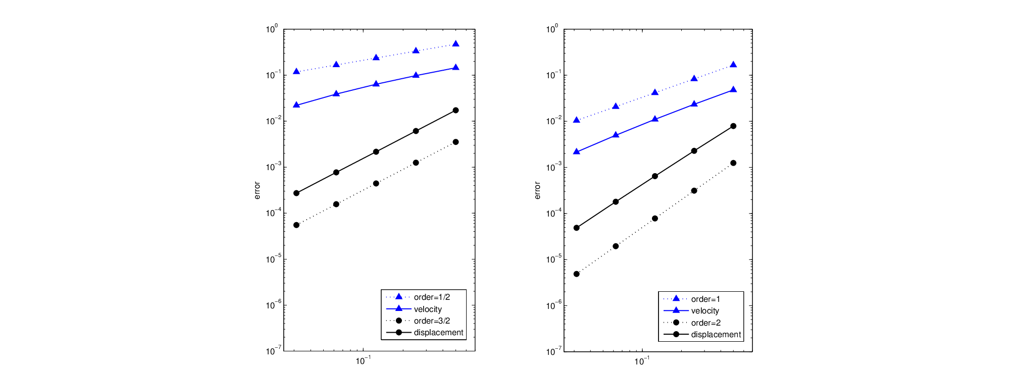
In the following experiments, we aim to test mean-square approximation errors as theoretically measured in (4.3), (4.4), (4.17) and (4.18). The expectation is approximated by the Monte-Carlo approximation, using path simulations. As the first task, we examine the spatial approximation errors and , with the endpoint fixed. The “true” solutions , are identified with numerical ones using small step-sizes . The numerical approximations under various spatial mesh sizes are achieved via time-stepping with . The resulting computational errors are listed in Table 1, where two kinds of noises are considered including the space-time white noise case () and the trace-class noise case (). To clearly see the convergence rates, we depict in Figure 1 the errors versus mesh sizes in logarithmic scale. As expected, the slopes of the errors (solid lines) and those of the reference dashed lines match well. More formally, the finite element spatial approximation errors in the space-time white noise case () exhibit convergence rates of order for the displacement and order for the velocity, which coincides with our previous theoretical findings in Theorem 4.1 when . For the other case ( and ), the errors show the predicted rates of order for the displacement and order for the velocity (see the right plot in Figure 1).
| 0.017262 | 0.144681 | ||
| 0.006098 | 0.097764 | ||
| 0.002158 | 0.063434 | ||
| 7.694527e-004 | 0.038866 | ||
| 2.723050e-004 | 0.022045 | ||
| 0.007918 | 0.048106 | ||
| 0.002289 | 0.023401 | ||
| 6.467743e-004 | 0.011036 | ||
| 1.800250e-004 | 0.004982 | ||
| 4.888214e-005 | 0.002160 |
Next, we proceed to tests on the convergence rates of temporal approximations. To this end, we fix and measure and for five different time stepsizes . In order to obtain , we perform time-stepping using small time stepsize . In Table 2 we present the computational errors for the two noise cases and . Similarly as before, these approximation errors are plotted versus time step-sizes in Figure 2, where one can easily observe the expected convergence rates. For example, in the trace-class noise case when , the approximation errors for the displacement and the velocity decrease at slopes of and , respectively, as the time step-sizes decrease. Also, convergence rates of order and are detected for the displacement and the velocity in the space-time white noise case (see the left plot in Figure 2). All in all, the above observations are all consistent with the previous theoretical results.
| 0.006226 | 0.166427 | ||
| 0.004302 | 0.141315 | ||
| 0.002560 | 0.116514 | ||
| 0.001332 | 0.091829 | ||
| 6.853130e-004 | 0.071157 | ||
| 0.003446 | 0.068094 | ||
| 0.002356 | 0.052651 | ||
| 0.001377 | 0.038405 | ||
| 6.993377e-004 | 0.025994 | ||
| 3.512776e-004 | 0.017476 |

Acknowledgments
Part of this work was done when the authors attended a seminar on stochastic computations at AMSS, Beijing. The authors want to thank Prof. Jialin Hong for his kindness and help during their stay.
References
- [1] A. Andersson and S. Larsson. Weak convergence for a spatial approximation of the nonlinear stochastic heat equation. arXiv preprint arXiv:1212.5564v3, 2013.
- [2] R. Anton, D. Cohen, S. Larsson, and et al. Full discretisation of semi-linear stochastic wave equations driven by multiplicative noise. arXiv preprint arXiv:1503.00073, 2015.
- [3] Y. Cao and L. Yin. Spectral galerkin method for stochastic wave equations driven by space-time white noise. Communications on Pure and Applied Analysis, 6(3):607, 2007.
- [4] D. Cohen, S. Larsson, and M. Sigg. A trigonometric method for the linear stochastic wave equation. SIAM J. Numer. Anal., 51(1):204–222, 2013.
- [5] D. Cohen and L. Quer-Sardanyons. A fully discrete approximation of the one-dimensional stochastic wave equation. IMA Journal of Numerical Analysis, page doi:10.1093/imanum/drv006, 2015.
- [6] G. Da Prato and J. Zabczyk. Stochastic equations in infinite dimensions, volume 152. Cambridge university press, 2014.
- [7] W. Fitzgibbon. Strongly damped quasilinear evolution equations. Journal of Mathematical Analysis and Applications, 79(2):536–550, 1981.
- [8] E. Hausenblas. Weak approximation of the stochastic wave equation. Journal of computational and applied mathematics, 235(1):33–58, 2010.
- [9] L. Jacobe de Naurois, A. Jentzen, and T. Welti. Weak convergence rates for spatial spectral galerkin approximations of semilinear stochastic wave equations with multiplicative noise. arXiv preprint arXiv:1508.05168, 2015.
- [10] F. Jiang, C. Huang, and X. Wang. Stochastic exponential integrator for finite element spatial discretization of stochastic elastic equation. Computers & Mathematics with Applications, 69(8):817–827, 2015.
- [11] M. Kovács, S. Larsson, and F. Lindgren. Weak convergence of finite element approximations of linear stochastic evolution equations with additive noise. BIT, 52(1):85–108, 2012.
- [12] M. Kovács, S. Larsson, and F. Lindgren. Weak convergence of finite element approximations of linear stochastic evolution equations with additive noise ii. fully discrete schemes. BIT, 53(2):497–525, 2013.
- [13] M. Kovács, S. Larsson, and F. Saedpanah. Finite element approximation of the linear stochastic wave equation with additive noise. SIAM Journal on Numerical Analysis, 48(2):408–427, 2010.
- [14] S. Larsson, V. Thomée, and L. B. Wahlbin. Finite-element methods for a strongly damped wave equation. IMA journal of numerical analysis, 11(1):115–142, 1991.
- [15] P. Massatt. Limiting behavior for strongly damped nonlinear wave equations. Journal of Differential Equations, 48(3):334–349, 1983.
- [16] V. Pata and M. Squassina. On the strongly damped wave equation. Communications in mathematical physics, 253(3):511–533, 2005.
- [17] R. Qi and X. Yang. Weak convergence of finite element method for stochastic elastic equation driven by additive noise. Journal of Scientific Computing, 56(3):450–470, 2013.
- [18] R. Qi, X. Yang, and Y. Zhang. Full-discrete finite element method for the stochastic elastic equation driven by additive noise. Numerical Methods for Partial Differential Equations, 29(6):1946–1962, 2013.
- [19] L. Quer-Sardanyons and M. Sanz-Solé. Space semi-discretisations for a stochastic wave equation. Potential Analysis, 24(4):303–332, 2006.
- [20] V. Thomée. Galerkin finite element methods for parabolic problems. Springer-Verlag, 2006.
- [21] V. Thomée and L. Wahlbin. Maximum-norm estimates for finite-element methods for a strongly damped wave equation. BIT Numerical Mathematics, 44(1):165–179, 2004.
- [22] J. B. Walsh. On numerical solutions of the stochastic wave equation. Illinois Journal of Mathematics, 50(1-4):991–1018, 2006.
- [23] X. Wang. An exponential integrator scheme for time discretization of nonlinear stochastic wave equation. J. Sci. Comput., 64(1):234–263, 2015.
- [24] X. Wang, S. Gan, and J. Tang. Higher order strong approximations of semilinear stochastic wave equation with additive space-time white noise. SIAM Journal on Scientific Computing, 36(6):A2611–A2632, 2014.
- [25] Y. Yan. Galerkin finite element methods for stochastic parabolic partial differential equations. SIAM journal on numerical analysis, 43(4):1363–1384, 2005.