Error Propagation of the Track Model and Track Fitting Strategy for the Iron CALorimeter Detector in India-based Neutrino Observatory Note: This work is submitted on behalf of INO collaboration

Journal: Computer Physics Communications

Kolahal Bhattacharya Email: kolahalb@tifr.res.in Corresponding author: Corresponding author Arnab K Pal Gobinda Majumder Naba K Mondal Address: Department of High Energy Physics, INO-Group (HECR Section), Tata Institute of Fundamental Research, 1-Homi Bhabha Road, Colaba, Mumbai-400005, India

Abstract

A Kalman filter package has been developed for reconstructing muon $(\mu^{\pm})$ tracks (coming from the neutrino interactions) in ICAL detector. Here, we describe the algorithm of muon track fitting, with emphasis on the error propagation of the elements of Kalman state vector along the muon trajectory through dense materials and inhomogeneous magnetic field. The higher order correction terms are included for reconstructing muon tracks at large zenith angle $\theta$ (measured from the perpendicular to the detector planes). The performances of this algorithm and its limitations are discussed.

Keywords:

Kalman filter , track fitting , magnetized iron calorimeter
PACS: 07.05.Kf , 29.40.Vj , 29.40.Gx

1 Introduction

Fitting a charged particle’s track through dense materials and inhomogeneous magnetic field is a well-known problem in High Energy Physics experiments. This is achieved by a recursive least square method, known as the Kalman filter [1]. For linear systems, this filter gives the best possible estimate with no bias and minimum variance [2]. However, for non-linear systems (like track fitting), there is no optimal estimator. The principles of the Kalman filter are generalized for constructing an extended Kalman filter [3] or an unscented Kalman filter [4]. Typically, an extended Kalman filter is used for track fitting by which one can extract the information of charge and momentum of the particle.

The Iron CALorimeter (ICAL) detector proposed by India-based Neutrino Observatory (INO) Collaboration [5] will observe atmospheric neutrinos $(\nu)$ through a 50 kiloton magnetized iron tracking calorimeter. The detector comprises three modules, each of dimension $16\rm{m}\times 16\rm{m}\times 14.4\rm{m}$ (Fig. 1(a)). These modules have 150 active detector planes, sandwiched between 151 iron slabs of thickness 5.6 cm. Each active plane in a module is made up of sixty four (64) $2\rm{m}\times 2\rm{m}$ Resistive Plate Chamber (RPC) detectors [6]. The current coils (Fig. 1(a)) generate magnetic field (Fig. 1(b)) inside the iron slabs. Charge current (CC) $\nu$ interactions will produce muons, electrons and hadrons which will pass through the detector and will give signals at the RPC strips.

The simulation effort for ICAL experiment begins with coding the detector geometry with the GEANT4 [7] tool-kit and by implementing the magnetic field map. The signals left by any particle in RPC detectors along its track are digitized to form hits in a rectangular ICAL coordinate system (Fig. 1(a)). The hits due to muon, a minimum ionizing particle, can be joined to form a track candidate. A track candidate needs to have minimum five hits in consecutive active layers to be defined as a muon track. The Kalman filter is used to fit this track.

On the other hand, hadron hits form a shower which might be calibrated with rather poor resolution [8]. Electrons also generate showers quickly and within 4- 5 iron layers they get absorbed. Therefore, it is not possible to reconstruct electrons. Thus, good reconstruction of muon is very important in this experiment.

A Few previous attempts [9, 10] of designing a muon track fitting package were not very successful. Muon tracks with vertices smeared over a large volume of the detector (beyond the central $8\rm{m}\times 8\rm{m}$ region of uniform magnetic field (Fig. 1(b))) were found prone to poor reconstruction. In reconstructed momentum distributions long tails were observed and charge identification efficiencies were poor as well. The aim of the current work is to design an algorithm with improved and stable performance of muon track fitting.

The main goal of the experiment is to resolve the neutrino mass hierarchy problem [11, 12]. It can also carry out the precision measurement analysis of atmospheric neutrino mixing parameters: $\Delta m^{2}_{32}$ and $\sin^{2}\theta_{23}$ . So far, these analyses have been done using simple assumptions of detector response [13, 14]. Recent studies [15, 16] were also done based on the detector performance of muon reconstruction, tabulated in the form of a look up table [10] that was generated by fitting Monte Carlo (MC) muon tracks with vertices smeared across the central $8\rm{m}\times 8\rm{m}$ region of central module of the ICAL detector. The event-by-event analysis of the reconstructed data has not yet been performed. This work is of relevance from that aspect also.

We begin by reviewing the problem of track following with Kalman filter in section 2. Next we explain the track following algorithm along the track in section 3. In section 4, we give the formulae for the error propagation of the track parameters. In section 5 the performance of the track following code and its limitations are presented and discussed.

2 Kalman Filter

In the ICAL experiment, the active detector planes are at predefined $z$ coordinates. In such a case, the state vector ${\bf x}=(x,y,t_{x},t_{y},q/P)^{T}$ at each detector plane $z$ is very convenient to work with. The elements $x(z_{k})$ and $y(z_{k})$ are the coordinates of a hit at the $k^{th}\ z$ plane, expressed in global ICAL coordinates. The charge $q$ of the particle and its momentum $P$ at $k^{th}\ z$ plane are included in the signed inverse momentum element $q/P$ . The corresponding slopes $t_{x}(z_{k})$ and $t_{y}(z_{k})$ are given as $t_{x}=dx/dz$ and $t_{y}=dy/dz$ . These slopes are related to the zenith angle $\theta$ and the azimuthal angle $\phi$ through the relations: $\cos\theta=\pm 1/{\sqrt{1+t_{x}^{2}+t_{y}^{2}}}$ and $\tan\phi=t_{y}/t_{x}$ respectively.

To employ a Kalman filter, we must propagate the mean value of the state $\bf{x}$ along with its associated errors [17, 18]. The filter routine then yields the near-optimum estimate of the state parameters. The convergence is achieved by attributing measured importance to both the observed data as well as the mathematical model giving the prediction. The steps for this are given below.

2.1 Basic Definitions of Kalman Filtering

The equation that describes the evolution of the state $\bf{x}$ from site $(k-1)$ to site $k$ , is given by

{{\bf{\bar{x}_{k}}}}=f_{k-1}({\bf{\bar{x}_{k-1}}})+{\bf{w_{k-1}}}

(1)

The bar symbol indicates the true values. Here $f_{k-1}$ is a propagator function that corresponds to a smooth deterministic motion in the absence of any random process noise $\bf w_{k-1}$ . In a dense medium, the random noise comes from multiple Coulomb scattering and energy loss fluctuations [18]. The process noise covariance matrix is given by $Q_{k}=\langle\bf{w_{k}}\bf{w_{k}}^{T}\rangle$ . With an estimate $\bf{x_{k-1}}$ for any true state $\bf{\bar{x}_{k-1}}$ , the estimation error covariance matrix is given by [3]:

C_{k-1}=\langle({\bf{x_{k-1}}}-{\bf{\bar{x}_{k-1}}})({\bf{x_{k-1}}}-{\bf{\bar{x}_{k-1}}})^{T}\rangle

(2)

The detector measures the state ${\bf m_{k}}=(x(z_{k}),y(z_{k}))^{T}$ at every plane ( $z_{k}$ ) along the particle trajectory. The relation between the true state vector $\bf{\bar{x}_{k}}$ and the measured state at $k^{th}$ plane is given by the measurement equation:

{\bf{m_{k}}}=h_{k}({\bf{\bar{x}_{k}}})+{\bf{\epsilon_{k}}}

(3)

where ${\bf m_{k}}$ is the measured data, $h_{k}$ is the measurement function and $\bf{\epsilon_{k}}$ denotes the error associated with the measurement. As before, the measurement noise covariance is given as $V_{k}=\langle{\bf{\epsilon_{k}}}{\bf{\epsilon_{k}}}^{T}\rangle$ . It is assumed that the process noise and the measurement noise are Gaussian errors and $\langle Q_{k}\rangle=\langle V_{k}\rangle=0$ .

2.2 Prediction

The latest state estimate $\bf{x}$ is extrapolated from $(k-1)^{th}$ plane to $k^{th}$ plane in the absence of random noise:

{{\bf{x_{k}^{k-1}}}}=f_{k-1}({\bf{x_{k-1}}})

(4)

Here, $\bf{x_{k}^{k-1}}$ is the predicted state at $k^{th}$ plane from the measurements done up to $(k-1)^{th}$ plane. The function $f_{k-1}$ is non-linear in general. To propagate the mean value of the state vector, Runge Kutta 4 method or equations based on helix model [3] are used in tracking. More recent work was done by Gorbunov et. $al$ , who deduced an iterative analytic solution for $f_{k-1}$ [19]. We used this solution in our work. The propagation of the ( $5\times 5$ ) error covariance matrix $C$ is done as:

C_{k}^{k-1}=F_{k-1}\ C_{k-1}\ F_{k-1}^{T}+Q_{k-1}

(5)

Here, ${C_{k}^{k-1}}$ is the predicted error matrix at $k^{th}$ plane from the measurements done up to $(k-1)^{th}$ plane. The derivation of Eq.(5) from Eq.(1) requires us to define $F_{k-1}$ as the $5\times 5$ Jacobian matrix:

F_{k-1}=\frac{\partial f_{k-1}}{\partial\bf x_{k-1}}

(6)

The first term in Eq.(5) propagates the errors in the state from the $(k-1)^{th}$ plane to the $k^{th}$ plane. This is deterministic error propagation that comes from the magnetic field and the local slopes and momenta of the track. The ${5\times 5}$ process noise matrix term $Q_{k}$ adds the random errors (due to multiple scattering and energy loss fluctuations) to the total error.

2.3 Filtering

The next step is to minimize the incremental $\chi^{2}$ between $(k-1)^{th}$ plane to $k^{th}$ plane. The incremental $\Delta\chi^{2}$ is:

\Delta\chi^{2}=({\bf{x_{k}}}-{\bf{x_{k}^{k-1}}}){\left[C_{k}^{k-1}\right]}^{-1}({\bf{x_{k}}}-{\bf{x_{k}^{k-1}}})^{T}+({\bf{m_{k}}}-h_{k}({\bf{x_{k}}})){\left[V_{k}\right]}^{-1}({\bf{m_{k}}}-h_{k}({\bf{x_{k}}}))^{T}

(7)

The term ${\bf{x_{k}}}$ denotes the Kalman estimate with respect to which the $\chi^{2}$ should be minimized. The condition $\frac{\partial}{\partial{\bf{x_{k}}}}(\Delta\chi^{2})=0$ leads to Kalman estimate for state $\bf{x_{k}}$ at $k^{th}$ plane in terms of $(5\times 2)$ Kalman Gain matrix $K_{k}$ :

K_{k}=C_{k}^{k-1}\ H_{k}^{T}\left(H_{k}\ C_{k}^{k-1}\ H_{k}^{T}+V_{k}\right)^{-1}

(8)

where the projector matrix $H_{k}$ is a $(2\times 5)$ matrix given by $H_{k}=\frac{\partial\bf{m_{k}}}{\partial{\bf x_{k}^{k-1}}}$ . For ICAL experiment, the projector matrix has the following form:

\left(\begin{array}[]{ccccc}1&0&0&0&0\\ 0&1&0&0&0\end{array}\right)

and the $(2\times 2)$ measurement error matrix $V_{k}$ is:

\left(\begin{array}[]{cc}{\sigma_{x}}^{2}&0\\ 0&{\sigma_{y}}^{2}\end{array}\right)

where $\sigma_{x}=\sigma_{y}=\frac{d}{\sqrt{12}}$ , $d$ being the strip-width of RPC detector. In terms of Kalman Gain $K_{k}$ , the filtered state estimate for $k^{th}$ plane is:

{\bf{x_{k}}}={\bf{x_{k}^{k-1}}}+K_{k}({\bf{m_{k}}}-H_{k}{\bf{x_{k}^{k-1}}})

(9)

Similarly, the Kalman estimate for filtered error covariance $C_{k}$ is given by:

	$\displaystyle C_{k}$	$\displaystyle=(I-K_{k}H_{k})C_{k}^{k-1}$
		$\displaystyle=(I-K_{k}H_{k})C_{k}^{k-1}(I-K_{k}H_{k})^{T}+K_{k}V_{k}{K_{k}}^{T}$		(10)

Then, ${\bf x_{k}}$ and $C_{k}$ are used for extrapolation from $k^{th}$ plane to $(k+1)^{th}$ plane. We found Eq.(10) (Joseph’s form [20]) to be useful for our work.

3 Track Following

The track following algorithm is based on equations stated in section 2. The coordinates of the digitized ‘hit’ found closest to the vertex is used to initialize $(x,y)$ elements of the Kalman filter. Using hits in the first few planes, $(t_{x},t_{y})$ near the vertex is obtained and are used to initialize the corresponding elements. The element $q/P$ is initialized to zero, thereby nullifying any initial bias.

By taking steps $\Delta{z}$ in $z$ direction, the state vector ${\bf{x}}(z+\Delta{z})$ is predicted from the state ${\bf{x}}(z)$ . In every step, first the local material and magnetic field is found; then, the step size is decided. Inside iron layers, $\Delta{z}$ is set to 1 mm and in other materials $\Delta{z}$ is set according to their widths. Energy loss of the particle in a step is calculated using Bethe Bloch formula [21] along with density effect corrections. The prediction of the $q/P$ element of the state vector is done using the energy loss information in that material. Prediction of the other elements are performed using the formulae given in section 4.1. This way, the prediction of the state vector (Eq.(4)) is done. Once the current step is over, the next step uses the predicted state as the initial state for that step.

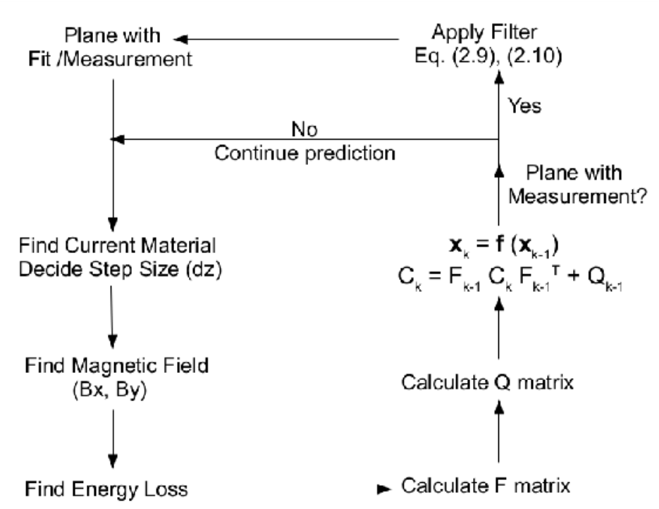
In every step, the propagator matrix (Eq.(6)) and the random noise matrix are calculated locally, using the material and the magnetic field. They are used to propagate the errors associated with the state elements. Now, as tracking is done from one hit to the next through a series of thick and dense materials, Eq.(5) cannot be directly used between two hits (previous work [10] was based on direct use of Eq.(5) between two hits). It has to be used repeatedly in each successive steps so that starting from $(k-1)^{th}$ hit, the random error contribution to the total error at $k^{th}$ hit becomes (Eq.(3.16) in [3]):

Q_{k-1}=\sum_{s=1}^{N-1}F_{m_{s},k}Q_{m_{s}}F_{m_{s},k}^{T}

(11)

In Eq.(11), $F_{m_{s},k}$ and $Q_{m_{s}}$ are the Jacobian matrix and the noise matrix for a small step. Then, the Kalman gain matrix $K_{k}$ (Eq.(8)) is calculated from $C_{k}^{k-1},V_{k}$ and $H_{k}$ . It is used to for obtaining filtered state [from Eq.(9)] and updated error covariance matrix [from Eq.(10)].

After all the hits in the muon track candidate have been filtered, the hits are processed in the reverse order using the same algorithm. This procedure ‘smooths’ the fitted track. The processing of hits in the forward and backward directions, completes one iteration. We have used four iterations, though for $>90$ % cases, the $\it fractional$ change in the desired state vector estimate were seen to become $<10$ % after the 2nd iteration. For tracks with only $4-5$ hits convergence was not at all achieved after four iterations.

4 Error propagation of track model

The set $(x,y,t_{x},t_{y})$ and the corresponding errors $(\delta{x},\delta{y},\delta{t_{x}},\delta{t_{y}})$ have been extrapolated on the basis of [19]. In this section, we shall give the formulae for error propagation of state parameters, to be used in the following propagator:

F_{k-1}=\begin{bmatrix}\frac{\delta[x(z_{e})]}{\delta x(z_{o})}&\frac{\delta[x(z_{e})]}{\delta y(z_{o})}&\frac{\delta[x(z_{e})]}{\delta t_{x}(z_{o})}&\frac{\delta[x(z_{e})]}{\delta t_{y}(z_{o})}&\frac{\delta[x(z_{e})]}{{\delta(\frac{q}{P}}(z_{o}))}\\ \frac{\delta[y(z_{e})]}{\delta x(z_{o})}&\frac{\delta[y(z_{e})]}{\delta y(z_{o})}&\frac{\delta[y(z_{e})]}{\delta t_{x}(z_{o})}&\frac{\delta[y(z_{e})]}{\delta t_{y}(z_{o})}&\frac{\delta[y(z_{e})]}{{\delta(\frac{q}{P}}(z_{o}))}\\ \frac{\delta[t_{x}(z_{e})]}{\delta x(z_{o})}&\frac{\delta[t_{x}(z_{e})]}{\delta y(z_{o})}&\frac{\delta[t_{x}(z_{e})]}{\delta t_{x}(z_{o})}&\frac{\delta[t_{x}(z_{e})]}{\delta t_{y}(z_{o})}&\frac{\delta[t_{x}(z_{e})]}{{\delta(\frac{q}{P}}(z_{o}))}\\ \frac{\delta[t_{y}(z_{e})]}{\delta x(z_{o})}&\frac{\delta[t_{y}(z_{e})]}{\delta y(z_{o})}&\frac{\delta[t_{y}(z_{e})]}{\delta t_{x}(z_{o})}&\frac{\delta[t_{y}(z_{e})]}{\delta t_{y}(z_{o})}&\frac{\delta[t_{y}(z_{e})]}{{\delta(\frac{q}{P}}(z_{o}))}\\ \frac{\delta[q/P(z_{e})]}{\delta x(z_{o})}&\frac{\delta[q/P(z_{e})]}{\delta y(z_{o})}&\frac{\delta[q/P(z_{e})]}{\delta t_{x}(z_{o})}&\frac{\delta[q/P(z_{e})]}{\delta t_{y}(z_{o})}&\frac{\delta[q/P(z_{e})]}{{\delta(\frac{q}{P}}(z_{o}))}\end{bmatrix}

(12)

In this matrix the suffix $e$ refers to the Extrapolated position ( ${\bf{r}}+{d\bf{r}}$ ) while the suffix $o$ refers to the Old position ${\bf{r}}$ . The last row is calculated more carefully for better convergence of $q/P$ parameter.

4.1 State and error propagation for $(x,y,t_{x},t_{y})$

We have calculated the expressions for $x(z_{e})$ , $y(z_{e})$ , $t_{x}(z_{e})$ and $t_{y}(z_{e})$ in terms of $\left[x,y,t_{x},t_{y},q/P\right](z_{0})$ and the magnetic field integrals, according to the model outlined in [19]. The analytic solutions were calculated up to the third order ( $n=2$ in $(q/P)^{n}$ with $n=0,1,2,3...$ ). They were utilized to find the derivatives required by the propagator matrix.

	$\displaystyle x(z_{e})$	$\displaystyle=x(z_{0})+t_{x}dz+h\left(t_{x}t_{y}S_{x}-(1+t_{x}^{2})S_{y}\right)+h^{2}[t_{x}(3t_{y}^{2}+1)S_{xx}$
		$\displaystyle-t_{y}(3t_{x}^{2}+1)S_{xy}-t_{y}(3t_{x}^{2}+1)S_{yx}+t_{x}(3t_{x}^{2}+3)S_{yy}]$		(13)

	$\displaystyle y(z_{e})$	$\displaystyle=y(z_{0})+t_{y}dz+h\left((1+t_{y}^{2})S_{x}-t_{x}t_{y}S_{y}\right)+h^{2}[t_{y}(3t_{y}^{2}+3)S_{xx}$
		$\displaystyle-t_{x}(3t_{y}^{2}+1)S_{xy}-t_{x}(3t_{y}^{2}+1)S_{yx}+t_{y}(3t_{x}^{2}+1)S_{yy}]$		(14)

	$\displaystyle t_{x}(z_{e})$	$\displaystyle=t_{x}+h\left(t_{x}t_{y}R_{x}-(1+t_{x}^{2})R_{y}\right)+h^{2}[t_{x}(3t_{y}^{2}+1)R_{xx}$
		$\displaystyle-t_{y}(3t_{x}^{2}+1)R_{xy}-t_{y}(3t_{x}^{2}+1)R_{yx}+t_{x}(3t_{x}^{2}+3)R_{yy}]$		(15)

	$\displaystyle t_{y}(z_{e})$	$\displaystyle=t_{y}+h\left((1+t_{y}^{2})R_{x}-t_{x}t_{y}R_{y}\right)+h^{2}[t_{y}(3t_{y}^{2}+3)R_{xx}$
		$\displaystyle-t_{x}(3t_{y}^{2}+1)R_{xy}-t_{x}(3t_{y}^{2}+1)R_{yx}+t_{y}(3t_{x}^{2}+1)R_{yy}]$		(16)

In the above expressions, $h=\kappa(q/P)\sqrt{1+t_{x}^{2}+t_{y}^{2}}$ where $\kappa=0.29979$ $GeVc^{-1}T^{-1}m^{-1}$ and $t_{x}$ and $t_{y}$ refer to $t_{x}(z_{0})$ and $t_{y}(z_{0})$ respectively. The factors $S_{...}$ and $R_{...}$ denote magnetic field integrals and $dz$ denotes $(z_{e}-z_{0})$ . The $B_{z}$ component of the ICAL magnetic field is zero and the field is in the $xy$ direction: $\vec{\bf{B}}=B_{x}(x(z),y(z)){\bf{\hat{x}}}+B_{y}(x(z),y(z)){\bf\hat{y}}$ . The field integrals are defined as [19]:

S_{i_{1}...i_{k}}=\int_{z_{0}}^{z_{e}}\int_{z_{0}}^{z_{e}}B_{i_{1}}(x(z_{1}),y(z_{1}))...\int_{z_{0}}^{z_{e}}B_{i_{k}}(x(z_{k}),y(z_{k}))dz_{k}...dz_{1}dz

(17)

and

R_{i_{1}...i_{k}}=\int_{z_{0}}^{z_{e}}B_{i_{1}}(x(z_{1}),y(z_{1}))...\int_{z_{0}}^{z_{e}}B_{i_{k}}(x(z_{k}),y(z_{k}))dz_{k}...dz_{1}

(18)

where $i_{1},i_{2}...$ etc denote $x,y,xx$ etc. These integrals were evaluated along the approximate particle trajectory. If the step size within iron is made reasonably small, magnetic field may be assumed to be constant along the step $dz$ and the calculation of the integrals becomes easier.

Table 1: Magnetic Field Integrals

$S_{x}$	$S_{y}$	$S_{xx}$	$S_{xy}$	$S_{yx}$	$S_{yy}$
$\frac{1}{2}B_{x}dz^{2}$	$\frac{1}{2}B_{y}dz^{2}$	$\frac{1}{6}B_{x}^{2}dz^{3}$	$\frac{1}{6}B_{x}B_{y}dz^{3}$	$\frac{1}{6}B_{x}B_{y}dz^{3}$	$\frac{1}{6}B_{y}^{2}dz^{3}$
$R_{x}$	$R_{y}$	$R_{xx}$	$R_{xy}$	$R_{yx}$	$R_{yy}$
$B_{x}dz$	$B_{y}dz$	$\frac{1}{2}B_{x}^{2}dz^{2}$	$\frac{1}{2}B_{x}B_{y}dz^{2}$	$\frac{1}{2}B_{x}B_{y}dz^{2}$	$\frac{1}{2}B_{y}^{2}dz^{2}$

The field integrals $S_{...}$ and $R_{...}$ were evaluated assuming that $B_{i}(x(z),y(z))$ vary very slowly along the track $(x_{particle}(z),y_{particle}(z))$ and may be assumed to be constant when integrating with respect to $z$ . This is true unless the particle is travelling almost parallel to the detector plane $(\theta\approx 90^{o})$ . The field integrals are given in Table 1. The effect of fringe field just outside the iron layer has been neglected in this work.

We also included the transverse variation of the field as in [22] (first addendum). This is because an error in the position $(x,y)$ leads to an error in the magnetic field. For example, error in $B_{x}$ is:

\delta{B_{x}}\approx\frac{\partial B_{x}}{\partial x}\delta x+\frac{\partial B_{x}}{\partial y}\delta y

(19)

The same is true for $B_{y}$ as well. This error in magnetic field gives an additional error of the direction of the track. As a result, there is an error $\delta{R_{x}}$ in the integral $R_{x}$ :

	$\displaystyle\delta{R_{x}}$	$\displaystyle=\int\delta{B_{x}(x(z),y(z))\ dz}$
		$\displaystyle\approx\left[\frac{\partial B_{x}}{\partial x}\ dz\right]\delta{x}+\left[\frac{\partial B_{x}}{\partial y}\ dz\right]\delta{y}$		(20)

Hence, from Eq.(15), the error of $t_{x}(z_{e})$ (to the first order in $h$ ) is given as:

$\displaystyle\delta t_{x}(z_{e})$	$\displaystyle=h\left[t_{x}t_{y}\frac{\partial B_{x}}{\partial x}-(1+{t_{x}}^{2})\frac{\partial B_{y}}{\partial x}\right]dz\ \delta x$
	$\displaystyle+h\left[t_{x}t_{y}\frac{\partial B_{x}}{\partial y}-(1+{t_{x}}^{2})\frac{\partial B_{y}}{\partial y}\right]dz\ \delta y$
	$\displaystyle+\left[1+h\left(t_{y}(1+\frac{{t_{x}}^{2}}{T^{2}})R_{x}-t_{x}(2+\frac{1+{t_{x}}^{2}}{T^{2}})R_{y}\right)\right]\delta t_{x}$
	$\displaystyle+h\left[t_{x}\left(1+\frac{{t_{x}}^{2}}{T^{2}}\right)R_{x}-t_{y}\left(\frac{1+{t_{x}}^{2}}{T^{2}}\right)R_{y}\right]\delta t_{y}$
	$\displaystyle+kT\ [t_{x}t_{y}R_{x}-(1+{t_{x}}^{2})R_{y}]\ \delta(\frac{q}{P})$	(21)

where $T=\sqrt{1+{t_{x}}^{2}+{t_{y}}^{2}}$ . Similarly, smooth deterministic errors in other parameters can also be evaluated. Then, it becomes a trivial task to obtain the first four rows of the propagator matrix Eq.(12). For instance, the term $\frac{\delta[t_{x}(z_{e})]}{{\delta(\frac{q}{P}}(z_{o}))}$ is equal to $kT\ [t_{x}t_{y}R_{x}-(1+{t_{x}}^{2})R_{y}]$ (from Eq.(21)). Terms of the order of $h^{2}$ were calculated using Mathematica [23].

4.2 Signed inverse momentum

Signed inverse momentum element $q/P$ has been extrapolated with Bethe-Bloch energy loss formula [24]. The corresponding error propagation has been done using techniques shown in EMC internal reports [25] (second addendum). However, the tracks have been assumed orthogonal to the detector planes there. This is not true in INO-ICAL detector which would observe the atmospheric neutrinos coming from all directions. So, the error propagation of $q/P$ is done more rigorously.

We want to find out the error $\delta(q/P)$ at a point $(x(z+dz),y(z+dz),(z+dz))$ of the track in terms of the error $\delta(q/P)$ at $(x(z),y(z),z)$ . We can write:

\delta(q/P)_{{{\bf{r}}(z+dz)}}=\delta(q/P)_{{\bf{r}}(z)}+\delta\left[d(q/P)\right]

(22)

The first term in Eq.(22) refers to the error in the estimate of $(q/P)$ , which was already there from $((x(z),y(z),z))$ . The second term denotes the average systematic error that creeps in due to the incorrect estimation of $q/P$ at $(x(z+dz),y(z+dz),(z+dz))$ from that at $((x(z),y(z),z))$ . It is possible to expand $d(q/P)$ as:

	$\displaystyle d(q/P)$	$\displaystyle=(q/P)_{{{\bf{r}}(z+dz)}}-(q/P)_{{\bf{r}}(z)}$
		$\displaystyle=f({{\bf{r}}(z+dz)})-f({\bf{r}}(z))$		(23)

where $f({\bf{r}})=q/P({\bf r})$ (which is known as the range-momentum relation). Muon CSDA (Continuous Slowing Down Approximation) range in $iron$ as function of muon momenta $P$ is known in the form of a numerical table [26]. We evaluate $d(q/P)$ in the track frame such that no cross term arises in the following expansion:

d(q/P)=f^{\prime}(l)dl+\frac{1}{2}f^{\prime\prime}(l)dl^{2}+\frac{1}{6}f^{\prime\prime\prime}(l)dl^{3}+...O(^{4})

(24)

where the arc length along the track is denoted by $l$ . In this equation, it is assumed that the higher order correction terms are negligibly small. This approximation does not hold good if the particle track is at a large zenith angle $\theta>60^{o}$ . In such cases, the derivatives of $f(l)$ are small, of course; however, the factors containing $dl$ and its exponents grow rapidly as $|dl|\approx\frac{dz}{\cos\theta}$ . The error in $d(q/P)$ can be given by (from Eq.(24)):

$\displaystyle\delta\left[d(q/P)\right]$	$\displaystyle=\delta\left\{f^{\prime}(l)dl\right\}+\delta\left\{\frac{1}{2}f^{\prime\prime}(l)dl^{2}\right\}+...$
	$\displaystyle=f^{\prime\prime}(l)\delta{l}\ dl+f^{\prime}(l)\ \delta(dl)+\frac{1}{2}f^{\prime\prime\prime}(l)\delta{l}\ dl^{2}+f^{\prime\prime}(l)\ dl\ \delta(dl)$
	$\displaystyle=\left\{f^{\prime\prime}(l)\ dl+\frac{1}{2}f^{\prime\prime\prime}(l)\ dl^{2}\right\}\delta{l}+\left[f^{\prime}(l)+f^{\prime\prime}(l)\ dl\right]\delta(dl)$	(25)

One must find $\delta{l}$ and $\delta(dl)$ correctly to obtain the error $\delta(q/P)_{{\bf{r}}(z+dz)}$ as a function of $\delta(q/P)_{{\bf{r}}(z)}$ and others. The factor $\delta{l}$ may be found from:

	$\displaystyle\delta(q/P)_{l}$	$\displaystyle=\delta{f(l)}$
		$\displaystyle=f^{\prime}(l)\delta{l}$		(26)

Thus, we have:

\delta{l}=\frac{\delta(q/P)_{l}}{f^{\prime}(l)}

(27)

The other term $\delta(dl)$ cannot be taken directly from EMC report $80/15$ as that calculation was done in SC frame $(x_{\perp},y_{\perp},z_{\perp})$ [18, 22] and we are working in a Cartesian reference frame. In Appendix, we show that the following holds in a Cartesian coordinate system [Eq.(41)]:

\begin{bmatrix}\delta{x}\\ \delta{y}\\ \delta{z}\end{bmatrix}_{{\bf{r}}(z+dz)}=\begin{bmatrix}1&d\phi&-\cos\phi\ d\theta\\ -d\phi&1&-\sin\phi\ d\theta\\ \cos\phi\ d\theta&\sin\phi\ d\theta&1\end{bmatrix}\begin{bmatrix}\delta{x}\\ \delta{y}\\ \delta{z}\end{bmatrix}_{{\bf{r}}(z)}+\begin{bmatrix}\delta(dx)\\ \delta(dy)\\ \delta(dz)\end{bmatrix}\,

(28)

in a Cartesian frame, where $\theta$ and $\phi$ are the zenith and azimuthal angles respectively. For ICAL experiment $\delta{z}_{z}=\delta{z}_{z+dz}=0$ , as the detector planes correspond to fixed $z$ coordinates. Thus, from Eq.(28), $\delta(dz)=-\cos\phi\ d\theta\ (\delta{x})_{z}-\sin\phi\ d\theta\ (\delta{y})_{z}$ . Then, $\delta(dl)$ may be expressed as:

$\displaystyle\delta(dl)$	$\displaystyle=\delta\left({dz\sqrt{1+{t_{x}}^{2}+{t_{y}}^{2}}}\right)$
	$\displaystyle=T\delta(dz)+dz\left(\frac{t_{x}}{T}(\delta\ t_{x})_{z}+\frac{t_{y}}{T}(\delta\ t_{y})_{z}\right)$
	$\displaystyle=T[-\cos\phi\ d\theta\ (\delta{x})_{z}-\sin\phi\ d\theta\ (\delta{y})_{z}]+dz\left(\frac{t_{x}}{T}(\delta\ t_{x})_{z}+\frac{t_{y}}{T}(\delta\ t_{y})_{z}\right)$
	$\displaystyle=\kappa\frac{q}{P}\ {dl}[B_{x}\ (\delta{x})_{z}+B_{y}\ (\delta{y})_{z}]+dz\left(\frac{t_{x}}{T}(\delta\ t_{x})_{z}+\frac{t_{y}}{T}(\delta\ t_{y})_{z}\right)$	(29)

where the last equality follows from Eq.(40). Hence, from Eq.(25) and Eq.(27), we can express $\delta[d(q/P)]$ in terms of $\delta(dl)$ as:

	$\displaystyle\delta\left[d(q/P)\right]$	$\displaystyle=\left\{\frac{f^{\prime\prime}(l)}{f^{\prime}(l)}\ dl+\frac{1}{2}\frac{f^{\prime\prime\prime}(l)}{f^{\prime}(l)}\ dl^{2}\right\}\delta({\frac{q}{P}})_{l}$
		$\displaystyle+\left[f^{\prime}(l)+f^{\prime\prime}(l)\ dl\right]\delta(dl)$		(30)

Hence, the error propagation for $q/P$ may be given as the following:

$\displaystyle\delta(q/P)_{l+dl}$	$\displaystyle=\left[1+\left\{\frac{f^{\prime\prime}(l)}{f^{\prime}(l)}\ dl+\frac{1}{2}\frac{f^{\prime\prime\prime}(l)}{f^{\prime}(l)}\ dl^{2}\right\}\right]\delta(q/P)_{l}$
	$\displaystyle+\kappa(f^{\prime}+f^{\prime\prime}\ dl)\ f(l)\ T\ dl\left[-B_{y}\ (\delta{x})_{l}+B_{x}\ (\delta{y})_{l}\right]$
	$\displaystyle+(f^{\prime}+f^{\prime\prime}\ dl)\ dz\left(\frac{t_{x}}{T}(\delta\ t_{x})_{l}+\frac{t_{y}}{T}(\delta\ t_{y})_{l}\right)$	(31)

We have used central difference formulae of order four (Richardson extrapolation) for calculating the derivatives $f^{\prime},f^{\prime\prime},f^{\prime\prime\prime}$ etc. with the help of [26]. We found that the convergence of $\frac{q}{P}$ to the desired values is very sensitive to the calculation of $\frac{\partial(\frac{q}{P})_{l+dl}}{\partial(\frac{q}{P})_{l}}$ term.

4.3 Random Error Contribution

So far we have discussed the average deterministic error terms. However, as indicated in Eq.(5), we must also account for the random errors due to multiple scattering and energy loss straggling. The multiple scattering matrix accounts for the random variation of the track elements $(x,y,t_{x},t_{y})$ over the average motion controlled by the magnetic field.

After crossing a distance $d$ the average angular variance in the track direction due to multiple scattering is given by [27]:

\langle\theta_{ms}^{2}\rangle=\frac{225\times 10^{-6}}{\beta^{2}P^{2}}\frac{d}{X_{s}}

(32)

where $X_{s}$ is related to the radiation length of the material. We used the formula given by Eq.(32) that keeps the angular variance proportional to the thickness $d$ . The expression given by Lynch [28] was used in previous work [10] to account for multiple scattering. But the presence of logarithmic term in that formula makes the calculation dependent on the step size, which is undesirable [18]. We applied the thick scatterer approximation to iron. The scattering from dense components of RPC like glass, copper and aluminium were also considered.

Apart from these, the fluctuations in the rate of energy loss also affect the motion of the muon to a great extent. The resulting muon energy loss distribution is a Landau (or a Vavilov) distribution. The corresponding random error propagation is done by using the covariance terms: $\rm cov[\xi,q/P]$ , where $\xi\in(x,y,t_{x},t_{y},q/P)$ . The term $\rm cov[q/P,q/P]$ is related to the variance of the truncated Landau distribution through [18]:

	$\displaystyle\rm cov[q/P,q/P]$	$\displaystyle=\frac{1}{P^{4}}\sigma^{2}(P)$
		$\displaystyle=\frac{E^{2}}{P^{6}}\sigma^{2}(E),$		(33)

We have evaluated $\sigma(E)$ from the Urban model [29] by sampling the number of of collisions suffered by the particle from a Poisson’s distribution (parametrized by the mean excitation potential of the material, the fraction $\alpha$ corresponding to the area of the truncated Landau distribution, and other parameters of the model). The fraction $\alpha$ was found to span rather wide range $(0.993$ - $0.999)$ if we wish to obtain unit standard deviation of the $q/P$ pull distribution in wide $P_{\mu}$ - $\theta_{\mu}$ range. In this paper, we report results obtained by setting $\alpha=0.998$ . The covariance term $\rm cov(x,q/P)$ was derived as below:

$\displaystyle\rm cov[x,q/P]$	$\displaystyle\equiv\rm cov[q/P,x]$
	$\displaystyle=\frac{\partial{x(P)}}{\partial{P}}\frac{\partial}{\partial{P}}\left[\frac{q}{P}\right]\sigma^{2}(P)$
	$\displaystyle=-\frac{q}{P^{2}}\frac{\partial{x(P)}}{\partial{P}}\sigma^{2}(P),$	(34)

where $x=x(P)$ is known from Eq.(13). Other cross terms were also evaluated this way using Eq.(14)-(16). Here we mention that $\langle\theta_{ms}^{2}\rangle$ and $\sigma(E)$ are already implemented in the free C++ track fitting library GENFIT [30], used by PANDA collaboration. The deterministic propagation of the Kalman parameters in GENFIT is based on EMC internal reports [22].

5 Results

In this section, we shall show the performance of the new Kalman filter algorithm coded on the basis of the formulae described in section 4. For this, 5000 muon ( $\mu^{\pm}$ ) tracks were simulated through virtual ICAL detector constructed with GEANT4 [7] tool-kit. The following study has been performed for muons of generator level momenta $P_{\mu}\in[1.0-10.0]$ GeV/c at $\cos\theta_{\mu}=0.95,0.75,0.55$ . The vertices of these tracks were uniformly smeared over the volume $(43\rm{m}\times 14.4\rm{m}\times 10\rm m)$ around the centre of the ICAL detector. This includes a major region of non-uniform magnetic field (Fig. 1(b)). An average strip multiplicity of 1.3 was taken in this work. The uncorrelated noise was enabled inside the detector. Hit detection efficiency of the central $1.88\rm{m}\times 1.88\rm{m}$ area of each RPC was assumed to be 99%. Rest portion of the RPC was assumed to belong to dead space.

5.1 Goodness of Fits

The goodness of typical fits is expressed by the Pull distributions and the chi squares ( $\chi^{2}$ ) of the fits. The pull of a fitted parameter $x$ is defined as:

P(x)=\frac{x_{reco}-x_{true}}{\sqrt{C_{xx}}}

(35)

Here $x_{true}$ is the true MC value and $x_{reco}$ is the reconstructed value. $C_{xx}$ is the diagonal element of the error covariance matrix, corresponding to the element $x$ .

For good fit, the pull distributions will have mean at zero and standard deviation equal to unity and the reduced $\chi^{2}$ distributions will have mean equal to unity. Apart from that, the p-value distributions of total $\chi^{2}$ should be reasonably uniform in the range [0-1.0]. This happens when the shape of the fitted $\chi^{2}$ distribution approaches a true $\chi^{2}$ probability distribution function. For this to happen, the prediction model should be good enough, the measurement errors should be Gaussian distributed and the measurements should be independent of each other.

In Fig. 3, we show these distributions for $\mu^{-}$ tracks of momentum $6$ GeV/c at zenith angle $\cos\theta=0.95$ . The error of an element $x$ has been represented by $\epsilon(x)$ in these figures. We see that the means of the pull distributions are close to zero and their standard deviations are close to one. The p-value distribution is more or less uniform in the range [0.1-0.8]. The peak near zero ( $p\rightarrow 0^{+}$ ) comes from the events lying in the tail of the fitted reduced $\chi^{2}$ distribution. The prediction model is not good enough for such tracks. On the other hand, the small heap near unity comes from events for which the measurements are highly correlated because of multiple scattering. This correlation leads to larger error ( $V_{k}+H_{k}C_{k}^{k-1}H^{T}_{k}$ ) which leads to smaller $\chi^{2}$ value. Indeed, we have seen that the heap becomes less prominent at higher momenta [ $\geq 10$ GeV/c] tracks for which the multiple scattering is less dominant. The reduced $\chi^{2}$ distributions were seen to have mean close to unity.

5.2 Performance at various input momentum ( $P_{\mu}$ ) and zenith angle ( $\cos\theta_{\mu}$ )

In this subsection, we show the variations of the means and the widths of the $q/P$ Pull distributions for various input $P_{\mu}$ and $\cos\theta_{\mu}$ values (Fig. 4(a), 4(b)). The corresponding charge identification efficiencies (CID(%)) is shown in Fig. 5(a). CID(%) has been defined as the % of events (having reduced chi square $<2.5$ ) with correct charge identification.

From Fig.s 4(a), 4(b) and 5(a), we see that the Kalman filter convergence of $q/P$ element is more or less comparable for $\mu^{-}$ and $\mu^{+}$ . The mean shift for them is symmetric about zero. In fact, as the zenith angle $\theta_{\mu}$ is increased, the accuracy of the $q/P$ convergence worsens gradually. The CID efficiency (Fig. 5(a)) also becomes poorer at higher $\theta_{\mu}$ (lower $\cos\theta$ ). On the other hand, if the generator momenta $P_{\mu}$ is increased, the standard deviation of the $q/P$ pull distribution shows almost linear (monotonic) increase. As mentioned before, Urban model [29] parameter $\alpha$ (section 4.3) was chosen such that the standard deviation of $q/P$ pull distribution comes close to unity for $P_{\mu}\in[4,9]$ GeV/c (as neutrino mass hierarchy sensitivity mostly comes from the muons of such momenta). The Means and standard deviations of the pull distributions for $(x,y,t_{x},t_{y})$ were also found to be consistent over a wide range of $P_{\mu}$ and $\cos\theta_{\mu}$ . Fig. 5(b) shows a $\mu^{-}$ track of $P_{\mu}=5$ GeV/c at $\cos\theta_{\mu}=0.35$ (that is, $\theta_{\mu}=69.5^{o}$ , measured from the perpendicular to the horizontal RPC planes). The filter convergence is found better if good enough number of measurements can be done along a track.

5.3 Comparison with the previous code

Here we shall compare the performance of the new algorithm with that of the existing code [10] and see what we have gained from the new algorithm. The following Fig. 6(a) shows the distribution of the reconstructed momenta obtained from the two codes for input momentum $P_{\mu}=5$ GeV/c at $\cos\theta=0.95$ . Fig. 6(b) shows the corresponding $\cos\theta$ distribution. In the following Table 2, we compare the rms errors of fitted $\theta_{\mu}$ and $P_{\mu}$ and charge identification efficiency(%) for input $\cos\theta=0.75$ as obtained from the two codes.

Table 2: Comparison of the two codes:

Code:-		Existing Code			Modified Code
P(GeV/c)	cos $\theta$	$rms(\theta_{\mu})$	$rms(P_{\mu})$	CID%	$rms(\theta_{\mu})$	$rms(P_{\mu})$	CID%
1.0	0.75	0.051	0.27	91.61	0.049	0.29	94.57
2.0	0.75	0.035	0.47	96.06	0.032	0.44	97.74
3.0	0.75	0.029	0.61	96.07	0.026	0.57	98.50
4.0	0.75	0.023	0.83	96.58	0.021	0.72	98.70
5.0	0.75	0.019	0.95	96.61	0.018	0.85	98.78
6.0	0.75	0.016	1.11	96.57	0.016	1.03	98.61
7.0	0.75	0.014	1.34	97.53	0.015	1.23	98.73
8.0	0.75	0.015	1.71	97.27	0.013	1.46	98.69
9.0	0.75	0.015	1.86	96.93	0.012	1.69	98.81
10.0	0.75	0.010	2.21	97.47	0.010	1.81	98.67

From the Fig.s 6(a), 6(b) and the Table 2, it is seen that implementing the algorithm (section 4) gave us considerably better results in terms of charge identification efficiency, accuracy and precision of the MC input parameters, compared to the previous code. The efficiency of reconstruction also increased.

5.4 Observations:

5.4.1 Fully/Partially Contained events

The reconstructed momentum distribution shows tails in both sides, more prominent at higher input momenta. They were found mostly due to the presence of Partially Contained (PC) tracks - for them, the resolution is poorer. In Fig. 7, we show the distribution for Fully Contained (FC) tracks superimposed to the Partially Contained (PC) tracks, for muons with momentum $P=5$ GeV/c at $\cos\theta_{\mu}=0.55$ . As expected, rms is much better for FC tracks. In Fig. 7, $\Delta{P}$ denotes $(P_{reconstructed}-P_{generator})$ .

5.4.2 Behaviour at low Momentum

The convergence for low momenta $P_{\mu}<1.5$ GeV/c events are usually poor, because in these cases less than $10-12$ hits are available. In Fig. 7, the reconstructed momentum distribution of $\mu^{+}$ of $P_{\mu}=1.0$ GeV/c at $\cos\theta_{\mu}=0.95$ is shown. Non-Gaussian tails are observed at such low momenta leading to poor momentum resolution.

6 Summary

In this work, we have tried to improve the existing muon track following code for ICAL experiment. That algorithm was based on a simple propagator matrix that had only first order correction terms [31]. We implemented higher order terms in random and deterministic error propagation formulae as obtained in section 4. The code is seen to produce better results compared to the existing code. The tail in the momentum distribution is suppressed and hence, the momentum resolution has improved. This is visible from Fig. 6(a). The reconstruction efficiency and charge identification efficiency also increased.

We have also performed the consistency checks on the final covariance matrix (that the matrix should be symmetric, the diagonal terms should be positive etc.). These checks turned out to be fine. It is seen that the convergence of Kalman parameters is very sensitive to accurate calculation of the fifth column of the propagator $F_{k-1}$ . The filter is seen to work over a wide range of momentum $P_{\mu}$ and direction $\cos\theta_{\mu}$ of muon. Except for small generator momenta ( $<1.5$ GeV/c) and/or low $|\cos\theta_{\mu}|$ ( $<0.4$ ), the filter is seen to produce reasonably accurate estimates. The fact that the mean of the $q/P$ pull distributions are close to zero in most of the cases implies that the average energy loss of the particle in different constituent materials has been accounted for correctly. Higher number of measurements (hits) along a track is found to lead to better convergence of track parameters.

However, at lower generator momenta and/or lower $|\cos\theta_{\mu}|$ , the number of hits are intrinsically small. Apart from that, multiple Coulomb scattering affects the track. In such scenarios, the filter performance is worse. Momentum resolution becomes poorer and charge identification efficiency degrades.

7 Acknowledgment

We thank Tata Institute of Fundamental Research where the Research and Developmental studies for the future ICAL detector is going on. The visualization software designed by D. Samuel was very useful. We also thank Y. P. Viyogi and D. Indumathi and S. Chattopadhyay for useful suggestions for improving the article. K.B. expresses gratitude to W. Wittek, for providing the details of error propagation along a particle trajectory in a magnetic field, which was the basis of the computation shown in section 4.2. The editor and the referee also helped us for improving the quality of the article with proper suggestions.

8 Appendix

The calculation of the propagator matrix in [22] was facilitated by the use of $SC$ coordinate system $(x_{\perp},y_{\perp},z_{\perp})$ , where $x_{\perp}$ is along the track direction and $y_{\perp}$ and $z_{\perp}$ are chosen to be locally orthogonal to the track. In this frame, the detector planes are the planes of constant $x_{\perp}$ , and therefore, $\delta(dl)$ in section 4.2 is exactly equal to $\delta(dx_{\perp})$ and both $\delta(dy_{\perp})$ and $\delta(dz_{\perp})$ are equal to zero. This frame is related to the Cartesian coordinates by the following equation [22]:

\begin{bmatrix}{x_{\perp}}\\ {y_{\perp}}\\ {z_{\perp}}\end{bmatrix}=\begin{bmatrix}\cos\lambda\ \cos\phi&\cos\lambda\ \sin\phi&\sin\lambda\\ -\sin\phi&\cos\phi&0\\ -\sin\lambda\ \cos\phi&-\sin\lambda\ \sin\phi&\cos\lambda\end{bmatrix}\begin{bmatrix}{x}\\ {y}\\ {z}\end{bmatrix}

(36)

where $\phi$ is the azimuthal angle and $\lambda$ is the dip angle and is related to the zenith angle $\theta$ as $\lambda=90^{o}-\theta$ . It has been shown that in the $SC$ system, that the infinitesimal displacement of the track in terms of infinitesimal deflections ( $d\lambda$ , $d\phi$ ) in the magnetic field can be written as:

\begin{bmatrix}{x^{\prime}_{\perp}}\\ {y^{\prime}_{\perp}}\\ {z^{\prime}_{\perp}}\end{bmatrix}=\begin{bmatrix}1&(\cos\lambda\ d\phi)&d\lambda\\ -\cos\lambda\ d\phi&1&\tan\lambda\ (\cos\lambda\ d\phi)\\ -d\lambda&-\tan\lambda\ (\cos\lambda\ d\phi)&1\end{bmatrix}\begin{bmatrix}{x_{\perp}}\\ {y_{\perp}}\\ {z_{\perp}}\end{bmatrix}

(37)

which corresponds to a deflection of angle ${d\vec{\alpha}}$ (due to magnetic field), given by:

d\vec{\alpha}=\begin{bmatrix}{\sin\lambda\ d\phi}\\ {-d\lambda}\\ {\cos\lambda\ d\phi}\end{bmatrix}

(38)

We want to find the corresponding equations in ICAL. With the help of $3\times 3$ Jacobian matrix in Eq.(36), we do similarity transformation of Eq.(37) and obtain:

\begin{bmatrix}{x^{\prime}}\\ {y^{\prime}}\\ {z^{\prime}}\end{bmatrix}=\begin{bmatrix}1&d\phi&-\cos\phi\ d\theta\\ -d\phi&1&-\sin\phi\ d\theta\\ \cos\phi\ d\theta&\sin\phi\ d\theta&1\end{bmatrix}\begin{bmatrix}{x}\\ {y}\\ {z}\end{bmatrix}

(39)

corresponding to an angle $d{\vec{e}}=\kappa\frac{q}{P}({\bf{e}}\times{\bf{B}})dl$ [Eq.(8) in [19] with ${\bf{e}}=(\frac{t_{x}}{T},\frac{t_{y}}{T},\frac{1}{T})$ where:

d\vec{e}=\begin{bmatrix}{\sin\phi\ d\theta}\\ {-\cos\phi\ d\theta}\\ {-d\phi}\end{bmatrix}=\kappa\frac{q}{P}\frac{1}{T}\begin{bmatrix}{-{B_{y}}}\\ {+{B_{x}}}\\ {(t_{x}B_{y}-t_{y}B_{x})}\end{bmatrix}dl

(40)

Eq.(40) says that the direction of the particle of momentum $P$ is rotated by the magnetic field $\bf B$ through an angle $d\vec{e}$ over a track length $dl$ . As the track of the particle is followed from ${{\bf{r}}(z)}$ to ${{\bf{r}}(z+dz)}$ an error $\delta$ in the estimation of the differential increment in the particle track length $dl$ happens due to curvature of the track in magnetic field (Fig. 8). From Eq.(29), we see that $\delta(dl)$ depends on $\delta(dz)$ .

\begin{bmatrix}\delta{x}\\ \delta{y}\\ \delta{z}\end{bmatrix}_{{\bf{r}}(z+dz)}=\begin{bmatrix}1&d\phi&-\cos\phi\ d\theta\\ -d\phi&1&-\sin\phi\ d\theta\\ \cos\phi\ d\theta&\sin\phi\ d\theta&1\end{bmatrix}\begin{bmatrix}\delta{x}\\ \delta{y}\\ \delta{z}\end{bmatrix}_{{\bf{r}}(z)}+\begin{bmatrix}\delta(dx)\\ \delta(dy)\\ \delta(dz)\end{bmatrix}\,

(41)

The errors $\delta x$ , $\delta y$ and $\delta z$ at ${{\bf{r}}(z)}$ propagate to ${{\bf{r}}(z+dz)}$ according to Eq.(39). Apart from these, the errors $\delta(dx)$ , $\delta(dy)$ and $\delta(dz)$ also creep in due to the curvature of the track. The total errors $\delta x$ , $\delta y$ and $\delta z$ at ${{\bf{r}}(z+dz)}$ are concisely given by Eq.(41).

We found the key relation Eq.(40) from Eq.(37) (valid in SC system) by using $(3\times 3)$ Jacobian (Eq.(36)) for coordinate transformation between the SC system and the Cartesian system. The propagator in the SC system [25], derived from helix model, was not directly used to express $\delta(dl)$ in terms of $\delta{x}$ etc. In fact, the propagator matrix $F_{k-1}$ in section 4 is based on the analytic formulae for track extrapolation. Of course, one can obtain the transformed propagator (equipped with these formulae) in SC/perigee system by using the $(5\times 5)$ Jacobian matrices (Eq. A24, A25, A28, A29) derived in [32]. They are very helpful when $F_{k-1}$ is not known in the required system, but is known in some other system.

References

[1] Rudolph Emil Kalman. A new approach to linear filtering and prediction problems. Transactions of the ASME–Journal of Basic Engineering, 82(Series D):35–45, 1960.
[2] R. Frühwirth, M. Regler, R. K. Bock, H. Grote, and D. Notz. Data Analysis Techniques for High-Energy Physics (Cambridge Monographs on Particle Physics, Nuclear Physics and Cosmology). Cambridge University Press, 2000.
[3] Fujii Keisuke. Extended kalman filter. The ACFA-Sim-J Group,, pages pp. 7, 15–17, 20, 2002.
[4] Eric A Wan and Rudolph Van Der Merwe. The unscented kalman filter for nonlinear estimation. In Adaptive Systems for Signal Processing, Communications, and Control Symposium 2000. AS-SPCC. The IEEE 2000, pages 153–158. IEEE, 2000.
[5] MS Athar, INO Collaboration, et al. a report of the ino feasibility study. Updated from the earlier Interim Report of May, 1:2005, 2006.
[6] Satyanarayana Bheesette. Design and Characterisation Studies of Resistive Plate Chambers. PhD thesis, INDIAN INSTITUTE OF TECHNOLOGY BOMBAY, 2009.
[7] S. Agostinelli et al. Geant4 - a simulation toolkit. Nuclear Instruments and Methods in Physics Research Section A: Accelerators, Spectrometers, Detectors and Associated Equipment, 506(3):250 – 303, 2003.
[8] Moon Moon Devi, Anushree Ghosh, Daljeet Kaur, SM Lakshmi, Sandhya Choubey, Amol Dighe, D Indumathi, Sanjeev Kumar, MVN Murthy, and Md Naimuddin. Hadron energy response of the iron calorimeter detector at the india-based neutrino observatory. Journal of Instrumentation, 8(11):P11003, 2013.
[9] Tapasi Ghosh and Subhasis Chattopadhyay. Track fitting by Kalman Filter method for a prototype cosmic ray muon detector. 2009.
[10] Animesh Chatterji, Kanishka Rawat, Meghna, and Tarak Thakore. Muon reconstruction look up table, v2. Technical report, INO Collaboration, 2012.
[11] Carlo Giunti and Chung W. Kim. Fundamentals of Neutrino Physics and Astrophysics. Oxford University Press, USA, 2007.
[12] Alexei Yu Smirnov. Neutrino mass hierarchy and matter effects. 2013.
[13] Abhijit Samanta. The Mass hierarchy with atmospheric neutrinos at INO. Phys.Lett., B673:37–46, 2009.
[14] Abhijit Samanta, Sudeb Bhattacharya, Ambar Ghosal, Kamales Kar, Debasish Majumdar, et al. A GEANT-based study of atmospheric neutrino oscillation parameters at INO. Int.J.Mod.Phys., A23:233–245, 2008.
[15] Anushree Ghosh, Tarak Thakore, and Sandhya Choubey. Determining the Neutrino Mass Hierarchy with INO, T2K, NOvA and Reactor Experiments. JHEP, 1304:009, 2013.
[16] Tarak Thakore, Anushree Ghosh, Sandhya Choubey, and Amol Dighe. The Reach of INO for Atmospheric Neutrino Oscillation Parameters. JHEP, 1305:058, 2013.
[17] R. Frühwirth. Application of Kalman filtering to track and vertex fitting. Nucl.Instrum.Meth., A262:444–450, 1987.
[18] A Fontana, P Genova, L Lavezzi, and A Rotondi. Track following in dense media and inhomogeneous magnetic fields. PANDA Report PVI01-07, pages pp. 3–6, 19–28, 2007.
[19] S. Gorbunov and I. Kisel. Analytic formula for track extrapolation in non-homogeneous magnetic field. Nucl.Instrum.Meth., A559:148–152, 2006.
[20] Juan Andrade Cetto and Alberto Sanfeliu. Environment Learning for Indoor Mobile Robots: A Stochastic State Estimation Approach to Simultaneous Localization and Map Building (Springer Tracts in Advanced Robotics). Springer, 2006.
[21] K. Nakamura et al. Review of particle physics. J.Phys., G37:075021, 2010.
[22] W Wittek. Propagation of errors along a particle trajectory in a magnetic field. Technical Report EMC-80-15, EMC-80-15-ADD-1, CERN, Geneva, 1980-81.
[23] Wolfram Res Mathematica. Inc., champaigne il, 2011.
[24] William R. Leo. Techniques for Nuclear and Particle Physics Experiments: A How-to Approach. Springer, 1994.
[25] W Wittek. Error propagation with energy loss: second addendum. Propagation of errors along a particle trajectory in a magnetic field. Technical Report EMC-80-15-ADD-2, CERN, Geneva, May 1982.
[26] Donald E. Groom, Nikolai V. Mokhov, and Sergei I. Striganov. Muon stopping power and range tables 10-MeV to 100-TeV. Atom.Data Nucl.Data Tabl., 78:183–356, 2001.
[27] R Frühwirth and M Regler. On the quantitative modelling of core and tails of multiple scattering by gaussian mixtures. Nuclear Instruments and Methods in Physics Research Section A: Accelerators, Spectrometers, Detectors and Associated Equipment, 456(3):369–389, 2001.
[28] Gerald R Lynch and Orin I Dahl. Approximations to multiple coulomb scattering. Nuclear Instruments and Methods in Physics Research Section B: Beam Interactions with Materials and Atoms, 58(1):6–10, 1991.
[29] Kati Lassila-Perini and László Urbán. Energy loss in thin layers in geant. Nuclear Instruments and Methods in Physics Research Section A: Accelerators, Spectrometers, Detectors and Associated Equipment, 362(2):416–422, 1995.
[30] C Höppner, S Neubert, B Ketzer, and S Paul. A novel generic framework for track fitting in complex detector systems. Nuclear Instruments and Methods in Physics Research Section A: Accelerators, Spectrometers, Detectors and Associated Equipment, 620(2):518–525, 2010.
[31] John Stuart Marshall. A study of muon neutrino disappearance with the MINOS detectors and the NuMI neutrino beam. PhD thesis, University of Cambridge, 2008.
[32] A Strandlie and W Wittek. Derivation of jacobians for the propagation of covariance matrices of track parameters in homogeneous magnetic fields. Nuclear Instruments and Methods in Physics Research Section A: Accelerators, Spectrometers, Detectors and Associated Equipment, 566(2):687–698, 2006.