Imaging parity-violating modes in the CMB
Abstract
Correlations of polarization components in the coordinate frame are a natural basis for searches of parity-violating modes in the Cosmic Microwave Background (CMB). This fact can be exploited to build estimators of parity-violating modes that are local and robust with respect to partial-sky coverage or inhomogeneous weighting. As an example application of a method based on these ideas we develop a peak stacking tool that isolates the signature of parity-violating modes. We apply the tool to Planck maps and obtain a constraint on the monopole of the polarization rotation angle degrees at We also demonstrate how the tool can be used as a local method for reconstructing maps of direction dependent rotation .
Subject headings
cosmic background radiation — cosmology: theory — polarization — techniques: polarimetricI. Introduction
The CMB provides a powerful test of deviations from standard physics. The energy fluctuations and polarization of photons released at last scattering carry information that is directly linked via simple, linear evolution to the primordial state of super horizon perturbations of the metric. In addition, CMB photons have traveled over cosmological distances to reach us, probing the nature of space-time along the way. The polarization of the CMB in, particular, is sensitive to a number of parity-violating mechanisms due to the opposite parity of and -modes [24, 41, 25].
These mechanisms can act either during the generation of primordial perturbations or during the propagation of the CMB photons through space at later times. The first possibility includes models of chiral gravity [30, 4, 15, 44] that explicitly break the parity between left and right handed primordial gravitational waves imprinted in super-horizon scales during inflation. The second includes the presence of parity-violating primordial magnetic fields [28, 42] or mechanisms that induce cosmic birefringence [12, 30, 17, 29] through the presence of new fields and interactions. Another possibility is the presence of spatial anisotropies during evolution of perturbations [6].
The simple consequence of all these mechanisms is that they result in correlations between the and -modes of the CMB polarization and between the -mode and total intensity . These correlations cannot exist unless parity is violated. The hope is therefore that a significant measurement of or correlations would be a “clean” indication of non-standard physics. The difficulty however is that these signals can also arise due to any experimental systematic that coherently rotates the polarization signal with respect to the true polarization of CMB photons. This can happen in experiments via either optical effects or mis-calibration of the polarization direction or efficiency of detectors.
With the advent of high signal-to-noise measurements of CMB polarization [39, 3, 2, 32, 26] we have entered an era where extensive test of parity-violating effects can be carried out along with a requirement for increasingly precise tests of polarization affecting systematics. Indeed, much work has gone into defining estimators of parity-violating statistics and their interaction with the experimental polarization calibration procedures [11, 35, 8, 27, 21, 40].
Estimation of the parity-violating signal has focused on the definition of optimal estimators based on the spherical harmonic expansion of the CMB Stokes parameters , , and into , , and -mode spherical harmonic coefficients. The focus on working in the , , basis is a naturally justified one since the correlation of these modes is where the signal of parity-violation is explicit. In contrast, it is not immediately obvious that correlations in the original , , and , coordinate frame modes can uniquely distinguish parity-violating signals as there is no one-to-one mapping of and modes to the parity-sensitive and modes. Working in harmonic space however, involves well-known complications due to the fact that the transformations involved are non-local. When a partial-sky coverage is imposed by scanning limitations or contamination by foregrounds the orthonormality of basis functions is reduced. This leads to mixing of power at different angular scales and mixing of and -modes. To deal with these unwanted effects one has to resort to complicated methods to statistically isolate the original harmonic modes [22, 10, 43].
In this work we point out that simple combinations of cross-correlations of Stokes parameters in the original coordinate frame are parity-violation sensitive and we show how these can be applied to data to yield an intuitive compression of the signals for parity-violating tests. Estimators based on coordinate frame correlations are simpler, and, in principle, more robust with respect to inhomogeneous noise, partial-sky coverage effects, and any polarization systematics. In fact, aside from efforts to detect non-standard physics, they can provide versatile tests of experimental systematics.
This paper is organised as follows. In section II we review how angular correlation functions of the Stokes parameters are related to parity-even and parity-odd angular power spectra. In section III we move to the small-angle limit and show how peak stacking can be used to obtain compressions of the signal that isolate parity-violating correlations. We validate our peak stacking tools using simulations of the CMB sky that contain varying degrees of parity-violation in the form of an overall polarization rotation. In section IV we use the tool to search for any parity-violating signal in the Planck maps. We discuss our results in section V.
II. Polarization Correlation Functions
The polarization of CMB photons on the full sky is described in terms of Stokes parameters, , , and . The scalar, total intensity component is expanded in spherical harmonics as
| (1) |
where is the unit direction vector on the sky. The Stokes parameters determining the direction of polarization on the sky are expanded on the basis of spin-2 spherical harmonics [46]
| (2) |
The and -modes transform distinctly under parity transformations with the gradient-like mode transforming with parity and curl-like mode transforming as . Given statistical isotropy the correlations in the expanded modes are diagonal and can be split into correlations that are insensitive to parity transformations
| (3) | ||||
| (4) | ||||
| (5) | ||||
| (6) |
and ones that only exist if the are parity-violating modes in the pattern
| (7) | ||||
| (8) |
The complex spin-2 field is a convenient measure for defining correlations in coordinate space. When considering correlations of the polarization between two lines of sight and we have to take into account that the polarization is defined with respect to a local basis, typically based on the local meridian. Rotating the polarization, in both directions, to a common frame defined by the geodesic connecting the two points on the sky subtending angles and with the original -axis at both points
| (9) |
with , one obtains a polarization definition that simplifies the relation between coordinate and harmonic space based correlations [33, 14]
| (10) | ||||
| (11) | ||||
| (12) | ||||
| (13) |
where is the cosine of the angle between the two directions and are the reduced Wigner rotation matrices [45]. These relations can be inverted to yield angular power spectra as functions of coordinate space correlations by using the orthogonality of the basis functions in the full-sky limit. Note that the and spectra contribute to the real part of both equations (12) and (13) but are multiplied by different basis functions. This is the reason why cut-sky effects have to be dealt with even when considering coordinate space correlation functions - the and mode contribution cannot be disentangled. The parity-violating components and however, only contribute to the imaginary parts of the correlations (11) and (12). In practice this means that we can use correlations obtained in the coordinate frame to isolate the signal due to parity-violating modes. Any estimate that does not rely on a harmonic transform greatly simplifies the problem of partial-sky coverage and inhomogeneous weighting.
The disadvantage is that the computation of correlation functions directly in the coordinate frame requires operations, where is the number of pixels in the map. Typically even methods that make use of the coordinate frame correlations (10)-(13) to simplify the effect of masking and noise weighting [14] actually estimate the correlations by transforming to the harmonic space. This is done in order to make use of the fast Fourier transforms in longitude.
In the following we will show how considering a subset of all possible correlations, those constrained to the neighbourhood of peaks in the Stokes parameters, can make use of the equations (10)-(13) to isolate the coordinate frame signal of parity-violating modes. We will leave the development of a more general framework exploiting the unconstrained correlations in the full-sky for future work.
III. Peak stacks
Peak stacking, or the averaging of a map in the neighbourhood of peaks in the map, has been used to determine the robustness of polarization measurements since large scale, polarization sensitive surveys appeared [27]. Recently they have been used to analyse more detailed morphology of the CMB around acoustic peaks in an attempt to constrain deviations from statistical isotropy [38]. Peak stacking provides a powerful visualization of the constrained correlation pattern around an acoustic peak of the CMB. It constitutes an intuitive tool that highlights the nature of the polarization as being precisely that expected from acoustic oscillations at last scattering. In the following we consider stacks around peaks in each of the Stokes parameters of polarised maps and show how these can be used to obtain parity-sensitive stacks that have simple relations to the parity-violating spectra and .
We will follow the notation and conventions used in [27] and consider explicit contributions and in and expand the phase factor in equation (9) in terms of sines and cosines. We develop the framework in the small-angle limit by considering the tangential projection, in coordinates (, ), around a point in the sky along direction . In this case the spin-, and spherical harmonics are replaced by two dimensional plane waves and their derivatives
| (14) | ||||
| (15) |
where (, ) is the wave vector in the plane-wave expansion with and and (, ) is the position vector in the tangential projection with and .
The total intensity field can now be expanded in the small-scale limit in the space of two-dimensional plane-waves
| (16) |
Following the conventions of [27, 25] we also expand the and Stokes fields as
| (17) | ||||
| (18) |
The coefficients and are the gradient and curl-like modes of the polarization component.
When stacking, or averaging fields around peak locations, we are calculating constrained (or biased) correlation functions [5]. We can write the stacking of a field at peaks in field in the ensemble limit as [27]
| (19) |
where is the total number of peaks in an area of the sky defined by the mask and is the number density of peaks in the field in the direction .
Introducing the dimensionless density contrast of peaks around the average peak density , we can write the stacking as
| (20) |
where is the fraction of the sky defined by the coverage mask and .
The effect of peak biasing can be calculated from first principles if is a Gaussian random field [23, 16, 27]. The density contrast can be written as a bias of the underlying field as
| (21) |
where is a scale-independent bias due to the selection of peaks of height , in units of the field’s standard deviation and is a scale-dependent bias due to the selection involving the curvature of the field. When considering stack averages therefore, we are actually evaluating a quantity that is second order in the statistics of the fields involved despite the average being first order in field units. Thus, despite the field having zero mean in the unconstrained limit, the constrained mean is not expected to vanish. The averages are related to the unconstrained correlation functions of the fields via a convolution with filters determined by the biasing functions such as in equation (21).
Introducing the short-hand and making use of the definition of the angular cross-correlations relations between statistically isotropic fields and
| (22) |
with and belonging to the set , , , the constrained mean of the temperature field about temperature peaks is related to the total intensity angular power spectrum as11 1 For a detailed summary of how is calculated we refer to Appendix B of [27].
| (23) |
where above and in the following are Bessel functions of order arising from the integration of the expressions over the plane wave azimuthal angle and we have introduced
| (24) |
as the Fourier domain counterpart of equation (21).
Similarly, one can show that suitably rotated combinations of and constrained means are related to the two cross-correlation angular power spectra
| (25) | ||||
| (26) |
The radial polarization projection of equation () removes the azimuthal dependence of the polarization pattern around the peaks and gives a distinct signal from parity-violating modes arising from any non-vanishing contribution. It is therefore a useful compression of the data along with a powerful visual check for the presence of any anisotropic or polarization rotation systematics [27, 38].
 |
 |
 |
 |
The constrained mean around and peaks can also yield useful projections of the polarization data that distinguish between parity-conserving and parity-violating modes. Following a similar derivation used for the expressions above, one can obtain the following useful combinations of averages around and peaks
| (27) | ||||
| (28) | ||||
| (29) | ||||
| (30) |
where we have introduced the notation .
Peak bias functions for the polarization fields are harder to calculate a priori since the original, unrotated and are generally correlated but in the limit of large we expect to recover 22 2 Alternatives would be to either stack around peaks in as done in [38] but this complicates the relations to the angular spectra, or work solely in the rotated complex variable which we leave for future work. In what follows we calculate using the same procedure described in Komatsu et al. [27] but with replaced by the total polarization power when computing the moments of the polarization field.
Under our assumption for the non-vanishing combinations in equations (27)-(29) simplify to
| (31) | ||||
| (32) | ||||
| (33) |
Two important points are readily apparent when considering correlations of this form. Firstly, in equations (31)-(33) we can see why the coordinate frame is not a natural one for separating out and -mode contributions. The correlations and contain distinct linear combinations of and but are filtered by Bessel functions of different order. This means that we can only separate and -modes in the full-sky limit by using the orthonormality of the basis functions [25, 14] - the spin-2 spherical harmonics in the full-sky case. In the flat-sky approximation we cannot use the orthogonality properties of the Bessel functions since the approximation breaks down at large angles. Thus and -modes are inevitably mixed when carrying out a partial-sky analysis leading to well-known separation issues. If we are interested in parity-violating modes however, provides a perfectly good estimate of the amount of correlation.
Secondly, the correlators are robust with respect to potential systematics. For example, in equations (27)-(29) we see that the contribution from mismatched peak biasing functions, proportional to , carry a specific dependence on the azimuthal angle while the signal of interest, proportional to in each case, is independent of . The signal can therefore be separated out by integrating over the dependence. In principle, this is the same for any contaminant that is not described by statistically isotropic correlations of the form shown in equations (3)-(8).
 |
 |
IV. Application
We now implement two separate methods based on peak stacking as simple examples of how we could use the correlators in equations (25)-(26) and (31)-(32) to constrain parity-violating modes in the CMB. To test our methods we use simulated CMB maps with parity-violating patterns induced by an explicit rotation of the original polarization pattern by an overall rotation angle . The rotation causes the mixing of power in , , and -modes and is described by the following angular power spectra [30, 17]
| (34) | ||||
| (35) | ||||
| (36) | ||||
| (37) | ||||
| (38) | ||||
| (39) |
where are the spectra of the original realization with vanishing and correlations.
Our second method will be a constraint on a direction–dependent rotation angle. To test the method we will use a simple toy model where the rotation angle varies as a dipole across the sky. In both cases we will also apply our estimation procedure to Planck CMB component maps.
IV.1. Average rotation
We use maps pixelised using the Healpix33 3 http://healpix.sourceforge.net [20] scheme at resolution . We generate realizations of the full-sky using the synfast tool at this resolution with input theoretical power spectra corresponding to the best-fit model in “base + r” fits reported in the latest Planck results [36]. A second set of realizations is generated using the rotated spectra in equations (34)-(39). We generate two realizations with rotation angles and degrees. All realizations are smoothed using a arcminute Gaussian window function and we have used the Planck total intensity and polarization transfer functions to smooth the theory to match the experimental beam effects in all cases.
We also use the Planck R2.0 SMICA , , and maps [1] down-graded to a common resolution of and smoothed by the same arcminute Gaussian window function as the realizations. We add the Half-Ring Half-Difference (HRHD) noise estimate to each of the realizations although the noise is significantly suppressed at our working resolution. Our polarization convention is different from that used in the Healpix package and corresponds to a change .
The analysis procedure is as follows: we run the Healpix hotspot tool to identify all peaks (both minima and maxima) in each set of , , and maps. We then take tiles, degrees wide, centred at each peak location and rotate them so that the peak is at a reference pixel. Each tile in , , and , is then added to separate stack averages after the monopole of each tile is subtracted [27, 38]. The subtraction minimises the effect of long-range correlations. We also exclude regions inside the mask defined by the SMICA confidence parameter. The stacks we obtain are an average of some 36,000 locations including both minima and maxima in all three Stokes parameters. We combine all maxima with thresholds above zero and the negative of all minima with thresholds below zero.
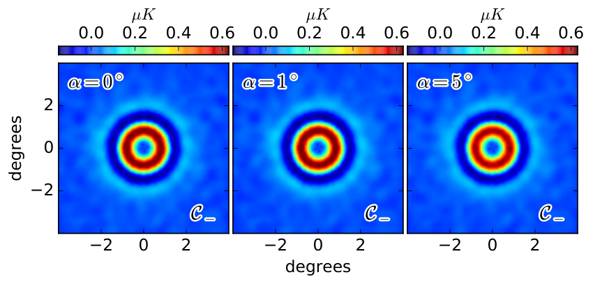
Figure 1 shows the peak stacks in , , , and for simulations with , , and degrees. For all cases the and stacks, that are not sensitive to parity-violating modes, display the expected radial envelope that decreases to the mean field limit as we move away from the peak. and only show a radial signal for the cases. For the degree case the stack, sensitive to modes shows a clear signal whereas for the respective stack the signal is close to the background level but clearly visible in the degree case.
For both and stacks, a signal with azimuthal dependence and amplitude roughly comparable to the background noise is visible close to the center of the stacks. This signal does not bias the estimate of parity-violation since it averages to zero when integrating in azimuthal angle .
The azimuthally averaged profiles for the stacks are shown in Figure 3. The stacks from simulated maps are consistent with the expected Bessel functions of zeroth and fourth order while the amplitude grows as a function of overall rotation . The figure shows an estimate of the background noise calculated using the standard deviation obtained by binning the variance of the stacks using the same procedure as the stacks themselves. In all cases the stacks that are only sensitive to the sum and difference and modes show highly significant signals. The signal from modes is significantly above the noise level for both simulations in the stack. The modes do not show up as strongly compared to the noise which is larger due to the large background induced by the correlation with the total intensity.
Figure 3 also includes model predictions based on the minimal CDM Planck best-fit model including tensors. The models are in excellent agreement with all the curves except for the case which peaks at and is sensitive to the residual noise bias. We have checked that adding an arbitrary white noise component to the model recovers the observed curve in this case. The agreement between the models and the observed and simulated curves validates our analytic treatment of the peak constrained stacks and in particular shows that our assumptions for the calculation of the bias function are robust.
The Planck SMICA map shows a hint of signal at a level degree. It is also consistent with a profile for arcminutes which is an indication that it may be sourced by an overall rotation. The mode is noisier than the channel. We can attempt to obtain an estimate for the overall rotation angle by fitting rotated models (37) and (39) to the Planck azimuthally averaged curves. As an estimate of the error in we use the variance maps accumulated during the stacking and co-added using the same azimuthal averaging. The correlations in the angular bins shown in Figure 3 are large. This can also be seen in the correlations, at the smoothing scale arminutes, of the noise fluctuations far from the central peaks in the stacked images. We therefore obtain our estimates using a simple fit assuming uncorrelated errors but on a much coarser binning of the azimuthally averaged profiles to minimize the correlations. We find that the estimate is stable for bins larger than arcminutes.
For a bin size equal to half the smoothing scale we obtain an joint estimate from fits to and of degrees at confidence. This is in broad agreement with a recent analysis using Planck data by [21].
IV.2. Direction-dependent rotation
 |
 |
 |
An analysis using peak stacks is not restricted to constraining the monopole of a possible rotation. In fact, if birefringence exists, there is no reason why it should induce a coherent rotation of the polarization angle over the entire sky. Recent constraints on birefringent effects have employed multipole based estimators for the direction dependent angle [40, 18] based on the estimator developed by [19]. The methods result in an estimate of the monopole expansion of the angle . These estimates based on measures of rotation in multipole space face the same problems with respect to inhomogeneous weighting and partial-sky coverage as conventional power spectrum estimation methods. In contrast an estimate based on peak stacks can provide a map of any potential signal without complications due to sky coverage and is only limited by the fact that peak stacking is not an optimal compression of all the information in the maps. It also has the advantage, shared with any coordinate space based measure, that it is more suitable to detect any signal that is compact on the sky. This makes it complementary to multipole based methods that are ideally suited to detect signals that are centred around certain angular scales or that have well defined, statistically isotropic, signatures.
As an example of how one could employ coordinate space based correlation function methods to constrain we modify our peak stacking pipeline to consider averages inside lower resolution pixels.The toy model we use to test this method is obtained by generating a map using the Healpix alm2map tool with a pure (, ) dipole mode with degrees as input. We use the map to apply a pixel dependent rotation of the polarization in the simulated Planck map with no initial parity-violating modes. The peak stacking procedure described in section IV.1 is repeated but the results are binned by low resolution pixels of . We then use the peak value of the estimate in each pixel, , as a tracer of the amount of average rotation in each low resolution pixel since gives the highest signal-to-noise determination of the rotation.
The results of this exercise are summarised in Figure 4 which shows how traces the input in the simulation. We also show the result of running this estimate on the SMICA map itself. The map for SMICA does not show any obvious signal although it is interesting to note that the two pixels at the extremes of the range in lie close to the excluded region that fails the SMICA confidence criterion. We leave a full analysis of the significance of these estimates for future work but in Figure 5 we show the binned distribution of pixel values outside and inside of the excluded region. All pixels that lie outside a bound defined by a best-fit Gaussian to the excluded pixels lie either inside the masked area or are immediately adjacent to it. The variance in the map also appears to be anisotropic with minima around the equatorial poles which correlates with the variance due to Planck’s scan strategy.
V. Discussion
We have shown how correlations of Stokes parameters of CMB maps can yield robust, local estimates of parity-violating signals. This can be useful when analysing maps to search for localised signals for which complementary harmonic based estimators are not ideal. Techniques based on coordinate frame correlation function estimators are therefore similar in spirit to many techniques used to investigate possible localised anomalies in the CMB (see [36] for a recent overview) which rely on coordinate frame statistics.
We used the correlators defined here to build simple tools to image parity-violating effects. We focused on peak stacking techniques as these provide a powerful compression of the acoustic signature in the polarization and are relatively easy to compute as opposed to the full, unconstrained correlations at the same resolution level. We have found the signal of parity-violation appears as expected in simulations where a non-zero effect was included and that our analytic estimates of the signal are in good agreement with the simulations. Our estimators run on Planck maps yield a limit on a sky-averaged rotation angle that is compatible with estimates in the literature obtained using different methods.
Our methods are not limited to the small angle limit we have adopted in this work. Peak stacking techniques focus are optimal for signals that modify the correlations on acoustic scales around a degree on the sky. They are well suited for along the line-of-sight birefringence effects. Other classes of parity-violating models however, may induce signals on larger angular scales if the effects were active during the inflationary phase in the early universe. In future work we will extend our methods to the full-sky. An additional advantage of this will be the exploitation of the full information in the maps. This will increase the signal-to-noise of any estimate and allows for much higher resolution reconstructions of maps such as those shown in Figure 4.
We used a simple exercise to show how the localised nature of these methods can be harnessed to reconstruct maps of spatially varying rotation angle. The example used a very large input rotation dipole as the signal to be reconstructed and the resulting map is much lower resolution than the input Planck maps. The choice of resolution was dictated by the limited number of peaks in the maps and we expect similar applications using the full-sky information will yield much higher resolution reconstructions.
Another advantage of methods based on coordinate frame correlations is the relatively straightforward implementation of noise weighting. We have not explored this here but we expect the results would be improved by correctly noise weighting the correlation estimators since the polarization information in current maps is still in the relatively low signal-to-noise regime. This would also help in targeting smaller angular resolutions in current and near-term polarization data.
On the small scales an interesting prospect is to explore how localised, peak stack estimators based on correlation functions of the polarization could help to extract lensing information from CMB maps. Gravitational lensing of CMB photons, now routinely measured (see [37] and references therein for a summary), leaves an imprint in the polarization signal that mixes and modes. Current estimates are based on higher-order correlations in harmonic space [34] and real space [13, 9]. Complementary techniques similar to those developed in this work may be feasible. In particular peak stacking may be ideally suited to isolate the lensing signal in a manner that is reminiscent of exploratory methods used to isolate the CMB lensing signal due to halos [7, 31].
References
- [1] Adam, R., et al. 2015, arXiv:1502.05956 [astro-ph.CO]
- [2] Ade, P., et al. 2015, Phys. Rev. Lett., 114, 101301
- [3] Ade, P. A. R., et al. 2014, Phys. Rev. Lett., 112, 241101
- [4] Alexander, S., & Martin, J. 2005, Phys. Rev. D, 71, 063526
- [5] Bardeen, J. M., Bond, J. R., Kaiser, N., & Szalay, A. S. 1986, Astrophys. J., 304, 15
- [6] Bartolo, N., Matarrese, S., Peloso, M., & Shiraishi, M. 2015, JCAP, 1507, 039
- [7] Baxter, E. J., et al. 2015, Astrophys. J., 806, 247
- [8] Brown, M. L., Ade, P., Bock, J., et al. 2009, ApJ, 705, 978
- [9] Bucher, M., Carvalho, C. S., Moodley, K., & Remazeilles, M. 2012, Phys. Rev., D85, 043016
- [10] Bunn, E. F., Zaldarriaga, M., Tegmark, M., & Oliveira-Costa, A. d. 2003, Phys. Rev., D67, 023501
- [11] Cabella, P., Natoli, P., & Silk, J. 2007, Phys. Rev., D76, 123014
- [12] Carroll, S. M. 1998, Physical Review Letters, 81, 3067
- [13] Carvalho, C. S., & Moodley, K. 2010, Phys. Rev., D81, 123010
- [14] Chon, G., Challinor, A., Prunet, S., Hivon, E., & Szapudi, I. 2004, Mon. Not. Roy. Astron. Soc., 350, 914
- [15] Contaldi, C. R., Magueijo, J., & Smolin, L. 2008, Phys. Rev. Lett., 101, 141101
- [16] Desjacques, V., Seljak, U., & Iliev, I. 2009, Mon. Not. Roy. Astron. Soc., 396, 85
- [17] Feng, B., Li, H., Li, M.-z., & Zhang, X.-m. 2005, Phys. Lett., B620, 27
- [18] Gluscevic, V., Hanson, D., Kamionkowski, M., & Hirata, C. M. 2012, Phys. Rev., D86, 103529
- [19] Gluscevic, V., Kamionkowski, M., & Cooray, A. 2009, Phys. Rev., D80, 023510
- [20] Gorski, K. M., Hivon, E., Banday, A. J., et al. 2005, Astrophys. J., 622, 759
- [21] Gruppuso, A., Gerbino, M., Natoli, P., et al. 2016, J. Cosmology Astropart. Phys, 6, 001
- [22] Hivon, E., Gorski, K. M., Netterfield, C. B., et al. 2002, Astrophys. J., 567, 2
- [23] Kaiser, N. 1984, Astrophys. J., 284, L9
- [24] Kamionkowski, M., Kosowsky, A., & Stebbins, A. 1997a, Phys. Rev. Lett., 78, 2058
- [25] —. 1997b, Phys. Rev., D55, 7368
- [26] Keisler, R., et al. 2015, Astrophys. J., 807, 151
- [27] Komatsu, E., et al. 2011, Astrophys. J. Suppl., 192, 18
- [28] Kosowsky, A., & Loeb, A. 1996, ApJ, 469, 1
- [29] Li, M., & Zhang, X. 2008, Phys. Rev., D78, 103516
- [30] Lue, A., Wang, L.-M., & Kamionkowski, M. 1999, Phys. Rev. Lett., 83, 1506
- [31] Madhavacheril, M., et al. 2015, Phys. Rev. Lett., 114, 151302, [Addendum: Phys. Rev. Lett.114,no.18,189901(2015)]
- [32] Naess, S., et al. 2014, JCAP, 1410, 007
- [33] Ng, K.-W., & Liu, G.-C. 1999, Int. J. Mod. Phys., D8, 61
- [34] Okamoto, T., & Hu, W. 2003, Phys. Rev., D67, 083002
- [35] Pagano, L., de Bernardis, P., de Troia, G., et al. 2009, Phys. Rev. D, 80, 043522
- [36] Planck Collaboration. 2015a, arXiv:1502.01589 [astro-ph.CO]
- [37] —. 2015b, arXiv:1502.01591 [astro-ph.CO]
- [38] —. 2015c, arXiv:1506.07135 [astro-ph.CO]
- [39] POLARBEAR Collaboration. 2014, Astrophys. J., 794, 171
- [40] —. 2015, arXiv:1509.02461 [astro-ph.CO]
- [41] Seljak, U., & Zaldarriaga, M. 1997, Phys. Rev. Lett., 78, 2054
- [42] Seshadri, T. R., & Subramanian, K. 2001, Phys. Rev. Lett., 87, 101301
- [43] Smith, K. M., & Zaldarriaga, M. 2007, Phys. Rev., D76, 043001
- [44] Sorbo, L. 2011, JCAP, 1106, 003
- [45] Varshalovich, D., Moskalev, A., & Khersonski, V. 1988, Quantum Theory of Angular Momentum: Irreducible Tensors, Spherical Harmonics, Vector Coupling Coefficients, 3nj Symbols (World Scientific Pub.)
- [46] Zaldarriaga, M., & Seljak, U. 1997, Phys. Rev., D55, 1830