Asymptotic Analysis of the Random-Walk Metropolis Algorithm on Ridged Densities
In this paper we study the asymptotic behavior of the Random-Walk Metropolis algorithm on probability densities with two different ‘scales’, where most of the probability mass is distributed along certain key directions with the ‘orthogonal’ directions containing relatively less mass. Such class of probability measures arise in various applied contexts including Bayesian inverse problems where the posterior measure concentrates on a sub-manifold when the noise variance goes to zero. When the target measure concentrates on a linear sub-manifold, we derive analytically a diffusion limit for the Random-Walk Metropolis Markov chain as the scale parameter goes to zero. In contrast to the existing works on scaling limits, our limiting Stochastic Differential Equation does not in general have a constant diffusion coefficient. Our results show that in some cases, the usual practice of adapting the step-size to control the acceptance probability might be sub-optimal as the optimal acceptance probability is zero (in the limit).
, , and ,
University College London??, University of Warwick??,
National University of Singapore??, Harvard University??
1 Introduction
Optimal scaling of Metropolis-Hastings (MH) algorithms in high dimensions and analysis of their asymptotic behavior has been a fruitful area of research in the last three decades. Initiated by [15], a long list of papers has been devoted to deriving the optimal scale of various local-move Markov Chain Monte-Carlo (MCMC) algorithms [17, 18, 12, 4, 2]. A main result in most of these works is identifying the proper scale for the proposal distribution at which the average acceptance probability is as a function of the dimension, and obtaining an associated diffusion limit. The limiting Stochastic Differential Equation (SDE) in all of the earlier works has a constant diffusion coefficient which uniquely characterizes its ‘speed measure’, with the latter being controlled by the step-size of the local-proposal and the average acceptance probability. For the Random-Walk Metropolis algorithm (RWM), maximizing the speed of the limiting diffusion leads to an average acceptance probability of 0.234. Thus the theoretical asymptotic analysis provides a simple optimality criterion that can be used as a guideline for practical implementation of these algorithms. Most of the papers cited above assume that the target measure is a product of one-dimensional densities - as this facilitates explicit calculation of the diffusion limit whose dynamics are independent of the state of other components. However, the product form assumption is not essential, and there are now a number of recent generalisations to target measures that are not of a product form [1, 3, 11, 13].
We adopt a different point of view in this paper, and study the behavior of the RWM algorithm on a class of target distributions that have ‘ridges’ in certain directions. Such target distributions arise in a number of examples in applied contexts. For instance, in Bayesian inverse problems, when the variance parameter in the likelihood model is small, the posterior distribution (as parametrized by the noise variance) will concentrate on a submanifold or along a hyperplane as the noise variance goes to zero. In contrast to the works cited above on scaling, the parameter space in our problems need not be high dimensional. The key issue pertaining to the mixing of MCMC algorithms in these contexts is that there is a natural separation of scale in the target distribution: a larger scale along certain key directions of interest where most of the probability mass is distributed and a smaller scale in the ‘orthogonal directions’ where there is relatively little mass. Thus in the context of previous works cited above, the role of the dimension is played by this scale. The contributions of this work are summarised as follows:
- i.
Motivated by inverse problems, we first describe a natural class of target distributions which have two scales (of magnitudes and ). Next, we study the RWM with step-sizes of the same scale for all co-ordinates. We focus on the case where the target distribution concentrates on a linear hyperplane as . Adapting the RWM steps in the direction of smaller scale , we derive a diffusion limit for the RWM for the co-ordinates with scale. In contrast with all previous results on diffusion limits of MCMC algorithms, our limiting SDE will in general have non-additive noise, i.e., the diffusion term will not have constant coefficients. We also look at the case when the step-size is allowed to vary according to the local curvature and obtain a corresponding diffusion limit. We show that diffusion limits can be useful in certain situations for providing optimality criteria in these problems. We mention that in the case of a linear manifold, the user can easily adapt the different RWM step-sizes along the various directions to obtain a very effective algorithm of cost . The real practical interest lies with non-linear structures. We have focused on a linear manifold to facilitate the development of theory. We also provide a conjecture for the diffusion limit in the practical case of a family of non-linear manifolds, but analytical derivations will require considerable future work.
- ii.
When the dimension of the manifold where the target measure concentrates lags that of the entire state space only by one, we find the usual practice of adapting the step-size to control the acceptance probability is not-optimal. In particular, our diffusion limits imply that a more efficient chain can be obtained by keeping a large step-size and allowing the acceptance probability to drop to zero. In this case we show that as , the optimally-scaled RWM algorithm does not converge weakly to a diffusion; rather it converges to a continuous-time Markov jump process.
- iii.
In contrast, when the dimension of the manifold where the target measure concentrates lags that of the entire state space by at least , we find that the diffusion regime is optimal. Intuitively, the cost of attempting large moves (as measured by small acceptance probability) is just too large in this case. In the critical case when the dimension of the manifold where the target measure concentrates lags that of the entire state space by exactly , the cost of low acceptance probability is of the same order as the benefit of larger moves, so that the optimal scaling strategy can vary depending on the specific form of the target density.
- iv.
As mentioned before, the most important practical benefit from deriving a diffusion limit is that it leads to an automated choice of the step-size: choose the step-size that maximizes the diffusion coefficient of the limiting SDE [15]. Doing so maximizes the speed measure of the limiting diffusion which in turn translates to maximizing the one-step expected jumping distance of the Markov chain at stationarity, or minimizing the first order auto-correlation for the chain. Since our limiting diffusions generally do not have a constant diffusion coefficient, this approach of maximizing the diffusion coefficient for choosing the step size is not valid any more. In general, there is no optimal value for the jump size of the RWM algorithm when applied to the target measures analyzed in this paper. We prove nevertheless that, if the jump size is allowed to be position dependent, optimality results can then be recovered. When the dimension of the coordinates with scale is large, our results yield a ‘local’ rule that generalize the standard global of [16], i.e., it is asymptotically optimal to tune the local jump size so that the local acceptance rate equals .
- v.
In general, practitioners should be aware that, when tuning the standard RWM algorithm, the general strategy consisting in choosing the largest jump size that yields an acceptance rate bounded away from a predetermined threshold (e.g., acceptance rate larger than ) is sometimes sub-optimal; indeed, our analysis shows that for ‘multiscale densities’, optimal strategies can yield arbitrarily small acceptance rates.
- vi.
Technically, our proofs for the diffusion limits are different from the usual optimal scaling literature, as the scale parameter in our target measure need not be related to the dimension. Our main argument relies on the fact that by suitably rescaling the co-ordinates corresponding to the scale , the RWM algorithm mixes in these directions at a much faster rate than its counterpart. This fast mixing on the Markov chain in the smaller scale will lead to an ‘asymptotic decoupling’ of the two scales which then will give the diffusion limit on the larger scales. The proof technique developed here could be applicable to other contexts and is thus of independent interest.
The class of target measures we analyze in this paper should be considered as surrogates for distributions arising from real applied problems where components have various length scales that differ by orders of magnitude. In Statistics, there are many such examples - we provide here a few, including our motivating scenario from Bayesian inverse problems.
- •
In inverse problems, situations where the posterior distribution concentrates in the neighbourhood of a non-linear manifold abound, see for example [14, 5, 9]. A typical situation involves the posterior distribution of a high-dimensional vector observed through a low-dimensional, possibly noisy, non-linear measurement function with ; the data collected is distributed as . As the intensity of the noise decreases to zero, the posterior distribution typically concentrates in a neighbourhood of thickness around the manifold .
- •
Suppose that we have a sequence of posterior distributions , indexed by the data size , where we can write with representing the components of the posterior which are identifiable while remains unidentifiable so that its standard deviation remains for increasing . For example, consider the posterior associated to observations of the diffusion process on ; as , only the volatility coefficient is identifiable. In the so-called regular case, we might expect the marginal posterior of to contract at rate for instance. Therefore it is very natural to see this scale divergence as .
- •
Consider the context of maximum likelihood estimation (MLE) for non-regular likelihood functions, For such problems, super-efficiency of MLEs is a well-known phenomenon, see for example [20], in which the standard deviation of the MLE shrinks to faster than for data size . It may be that super-efficiency applies only to some of the model parameters, leading to the kind of heterogeneously scaled target distributions we consider here. For concreteness, we consider the specific problem where the data is assumed to be drawn i.i.d from the model conditioned on . It is well-known that for this kind of example the posterior for contracts at the regular rate of while that for contracts at the much more rapid rate of . Thus again we get scale divergence as .
The paper is structured as follows. In Section 2 we describe the RWM algorithm for a density concentrating on a hyperplane with rate . In Section 3 we state the regulatory conditions and write the diffusion limits as . In Section 4, we prove the stated results. In Section 5 we prove a limiting result involving a Markov jump-process, when the step-sizes are order , so are not adapted to the size of the smallest co-ordinate. In Section 6 we describe in some detail a conjecture for generalizing our diffusion limit results in the context of non-linear manifolds. Throughout, we provide comments about the implications of the theoretical results. We finish with some conclusions and description of future work in Section 7.
2 Random-Walk Metropolis on Affine Manifold
As explained above, we prove analytical rigorous results in the case when the manifold is flat, i.e. an affine subspace of the general state space. We discuss later on in the paper extensions to more general manifold structures. We model the affine scenario as follows. We consider the target distribution , for integers and , with density with respect to the -dimensional Lebesgue measure
| (1) |
for a ‘small’ scalar . The -marginal has density independently of . This is a scaled version of the probability distribution . As , the support of the sequence of distributions concentrates on the linear subspace :
| (2) |
of dimension . Integer can sometimes be thought of as the dimension of the non-identifiability and the integer as the part of dimension that is fully specified. For instance, in a small-noise or increasing-data context, one can consistently estimate -parameters out of . Parameter can be thought of as the thickness of the support of at a neighbourhood of .
To obtain samples from we consider the RWM algorithm proposing moves
for a scaling factor , tuning parameter and noise . The factor determines the scales of the jumps of the RWM algorithm and the tuning parameter allows to control the acceptance rate of the algorithm. When the context is clear, we write simply instead of . For the purpose of analysis, we introduce the rescaled coordinate and the associate rescaled proposal ,
If then . To finish the description of the MCMC algorithm, we need to choose an accept-reject function . To obtain detailed balance w.r.t. , one can choose any -valued function satisfying the reversibility condition
| (9) |
The usual Metropolis-Hastings accept/reject correction corresponds to the choice . The move , or equivalently , is then accepted with probability
We work with a general accept-reject function as enforcing some differentiability condition removes several inessential technicalities from our proofs. Indeed, we assume in the remainder of this article the following regularity assumptions on .
Assumption 1.
The accept/reject function is differentiable. and are globally Lipschitz and bounded over the real line.
Assumption 1 could be relaxed. For example, one could deal with the standard Metropolis-Hastings ratio; this would involve dealing with the discontinuity of the derivative at 0, which is only a technical distraction that does not bring new insights into the behaviour of the algorithm and make the proofs much more opaque. Notice that any function satisfying the reversibility condition (9) is dominated by the Metropolis-Hasting function in the sense that the inequality holds for any . For the target density (1) the acceptance probability can be written analytically as where the function reads
| (10) |
The above proposal and acceptance probability give rise to the MCMC trajectory .
2.1 Notation
For we write (or sometimes ) to denote the conditional expectation . For functions , we write to indicate that the expectation is considered under the standardised law . We denote by the -norm, . We use the expression “” to indicate that for function we have . We use the symbol to indicate inequalities that hold under multiplication with a constant which does not depend on critical parameters implied by the context.
3 Diffusion Limit
We study in this section the behaviour of RWM, as , for a scaling factor of the form
| (11) |
Note that it is straightforward to prove that any other scaling factor such that would lead to an algorithm with an acceptance rate that decreases to zero as . This corresponds to an algorithm that proposes too large moves and such a context is investigated in Section 5. A scaling factor of the form (11) thus corresponds to the largest choice of jump-sizes that leads to an algorithm who acceptance rate does not degenerate to zero in the limit . To state one of our main results, we introduce the quantity
| (12) |
which corresponds to the limiting average acceptance probability, as , of the RWM algorithm when assuming stationarity for , conditionally on a fixed position for the -coordinate. One can easily verify (bounded convergence theorem) that
| (13) |
assuming . We prove a diffusion limit for the trajectory of the -coordinate, after considering a proper continuous time-scale for its discrete-time trajectory , where denotes the number of MCMC iterations. To this end, we define
Our main result states that the sequence of accelerated, continuous-time, càdlàg processes
| (14) |
converges weakly, as , to a non-trivial diffusion process; thus corresponds to the ‘diffusive time-scale’.
Remark 1.
For a given positive density function , for , and a scalar volatility function we introduce the function
| (15) |
Consider the stochastic differential equation (SDE):
| (16) |
where denotes -dimensional Wiener process. Under standard regularity assumptions the SDE (16) has a unique global solution and is reversible with respect to the law . The case corresponds to the Langevin diffusion .
To obtain our scaling limit, we assume the following regularity conditions for functions and involved in the specification of the density .
Assumption 2 (Regularity Conditions on ).
Functions and are differentiable and their derivatives are globally Lipschitz. Moreover, we assume that the distribution possesses finite second moments in the sense that
| (17) |
Assumption 2 is repeatedly used to control the error terms associated to the use of second order Taylor expansions; the second moment bound allows the use of the Cauchy-Schwarz inequality. Note that these assumptions could be relaxed in several directions at the cost of increasing complexity in the proofs; for example, one could assume only a polynomial growth on the derivatives and higher moments for . We also need the following assumption to control the behaviour of the diffusion limit identified below.
Assumption 3.
The function is bounded on and there is an exponent such that
The main theorem of this section is the following. The proof is given in Section 4.1.
Theorem 1.
Let be a fixed time horizon. Assume that the RWM algorithm is started in stationarity, , and Assumptions 1-3 hold. Then, as the sequence of processes defined via (2), (14) converges weakly in the Skorokhod space to the diffusion process specified as the solution of the stochastic differential equation:
| (18) |
for volatility function and initial position .
Under Assumption 3, the limiting diffusion (18) is well defined, does not explode in finite time, and has a unique strong solution. The assumption is as stated in [6, Ch. 4, Theorem 1.6]. Furthermore, Assumption 3 yields that for a smooth and compactly supported test function the function , with
| (19) |
the generator of the limiting diffusion (18), is -Holderian. The diffusive time scale implies that the algorithmic complexity of RWM grows as as the thickness approaches zero; see [19] for general results on the complexity analysis of MCMC algorithms through diffusion limits. In the case where the function does not depend on the -coordinate, the limiting acceptance probability does not depend on the local position , i.e. . In this case the optimal value for the parameter is given by . In the general case however, the optimal choice of will depend on the current -position.
3.1 Extending Theorem 1
We can also adopt slightly more general proposals where the variance of the proposals is allowed to depend on the current position. That is, the tuning parameter is now allowed to depend on the -coordinate:
We state the required assumptions on the function that allows the relevant diffusion limit results to hold.
Assumption 4 (Regularity Assumptions on ).
The function is positive, bounded away from zero and infinity. The first two derivatives of are bounded.
We choose to work in the limited setup of Assumption 4 so that the proof of the next theorem is a straightforward adaptation of Theorem 1. The accelerated version (14) of the -coordinate process again converges to a diffusion process.
Theorem 2.
Let be a fixed finite time horizon. Assume that Assumptions 2-4 hold and that the RWM algorithm is started in stationarity. As , the sequence of processes defined via (3.1), (14) converges weakly in the Skorokhod space to the diffusion process specified as the solution of the stochastic differential equation
| (26) |
The local volatility function is . The initial distribution is .
The only difference with Theorem 1 is the form of the volatility function . As before, the limiting distribution (26) is reversible with respect to and the Dirichlet form reads
| (27) |
Since the parameter is a function of the -coordinate, the optimal choice for the tuning parameter is
| (28) |
As described in [18], the choice (28) maximises the ESJD, the spectral gap of the limiting diffusion (26) and the asymptotic variance of MCMC estimators.
3.2 High-Dimensional Asymptotics and Local Rule
In this section, we investigate the behaviour of the optimal jumping rule in the regime where the dimensionality of the identifiability is large i.e. . We adopt the setting where the dimension remains fixed while the dimension grows to infinity. For simplicity, we postulate a product form for the -marginal density. That is, we investigate the sequence of densities
in the regime where and , with
where is such that for any the function is a proper density function on . We denote by the optimal value of the jump size when the -coordinate of the MCMC algorithm exploring stands at . With the obvious notations, the previous sections show that where
for an i.i.d. sequence of -valued random variables with distribution and an i.i.d. sequence of standard Gaussian random variables . We assume the following regularity conditions on the marginal density ; this is the equivalent of the conditions (A1) and (A2) of [15].
Assumption 5.
The density is twice differentiable, the function is Lipschitz continuous and the random variable with density is such that
A simple adaptation of Corollary of [15] yields that, under Assumption 5, we have
Corollary of [15] corresponds to the special case where a closed form expression for exists; for concreteness, we will also consider the special case although generalization to arbitrary accept/reject functions is straightforward. The function is maximized for such that (to three decimal places) [15]; in other words, as , the optimal jumping rule can be chosen such that the local acceptance rate at equals approximately . Indeed, the derivation of this rule-of-thumb relies on the product form assumption of the -marginal and is only valid in the asymptotic regime . Nevertheless, this type of analysis has been shown to be empirically and theoretically [4, 1, 3, 2, 11, 13] relevant to more general distribution structures.
4 Proof of Diffusion Limit
This section gives rigorous proofs of Theorems 1 and 2. The proof is based on [6, Ch. , Theorem ] which gives conditions under which the finite dimensional distributions of a sequence of processes converge weakly to those of a Markov process. [6, Ch. , Corollary ] provides further conditions for this sequence of processes to be relatively compact in the appropriate topology and thus establish weak convergence of the stochastic processes themselves.
4.1 Proof of Theorem 1
We first give a high-level description of the proof. We introduce an intermediate time scale for an exponent , and consider the sub-sampled process defined as
On this time-scale the -process evolves slowly (i.e. ) whereas the -process has the time to mix (i.e. is approximately independent from ). We define the continuous-time accelerated processes
| (29) |
See Fig.1 for a graphical representation of all four main processes involved in our derivations.
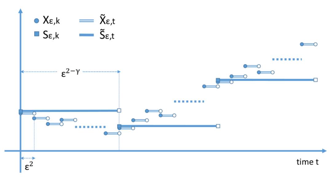
The proof is divided into two steps. First, we show that the process converges weakly in the Skorokhod topology to the diffusion (18). Then, we prove that the supremum norm
converges to zero in probability, establishing the weak convergence of the sequence itself towards the diffusion (18). We define some quantities needed in the sequel. Recall the definition in (19) of the generator of the limiting diffusion (18). Similarly, we denote by and the generators of the càdlàg processes and respectively. That is, let be the space of smooth functions with compact support; for any test function and vectors we have
Although the domain of is , functions and are defined on , as processes and are not Markovian with respect to their own filtration. The telescoping sum yields that
| (32) |
This identity is repeatedly used in the sequel. As a first step, we prove that for test function , generator converges, in an appropriate sense, to the quantity given by
| (33) |
where for notational convenience we have defined . Also, we have used the Laplacian notation . In general, does not correspond to the generator of a Markov process. Note that if is smooth with compact support, under Assumptions 1-2 we have that . We prove in Section A.1 the following result.
Proposition 1.
4.1.1 Weak convergence of to the limiting diffusion (18)
We start by proving that the weak convergence of towards the limiting diffusion (18) reduces to studying the behaviour of the difference between the approximate and limiting generators.
Proposition 2.
For clarity, the proof is divided into two main steps. First, one proves that the finite dimensional distributions of converge to those of the limiting diffusion. Secondly, one proves that the sequence is relatively weakly compact in the appropriate topology.
Convergence of the finite dimensional distributions of .
We follow closely [6, Ch. , Theorem and Corollary ]
and apply those results for the set of functions
.
Under Assumption 3, [6, Ch. , Theorem ] gives
that the closure of generates a Feller semigroup (corresponding
to the solution of the SDE) on the Banach space
of continuous functions vanishing at infinity.
Thus, all conditions at the statement of [6, Chapter , Theorem ]
are satisfied; it remains to prove part (e) of [6, Ch. , Corollary ].
Given an arbitrary test function , we
set
and .
We need to prove Equations - and of [6, Ch. , Theorem ] (Equation is trivially satisfied); that is, one must show that
for any , any times ,
and any functions that can be assumed to be bounded.
Indeed, [6, Ch. , Theorem ] shows that the above equations
involving the generators and expectations at infinitesimally small increments from instance
can imply convergence over finite times.
The first requirement follows from the boundedness of ;
the second requirement is implied by the stationarity of
,
Equation (35) and the fact that
(we have that from the boundedness of the gradient of the drift function of the limiting diffusion
on compact domains, since it is continuous from Assumption 3).
The third requirement is also implied from (35).
We have now proven the required convergence of the finite dimensional distributions
of to those of the solution of the limiting SDE (18).
Relative weak pre-compactness of .
We follow [6, Ch. , Corollary ].
First, we remark that the process is started at stationarity
and the space of smooth functions with compact support is an
algebra that strongly separates points.
As noted in the proof of [6, Ch. , Corollary ], the pair , with as defined above, in general does not belong to the approximate generator defined in Equation of [6, Ch. ] and one needs to consider instead the pair
to account for the fact that the process is a discrete time Markov chain (note here the typo in Equation (8.28) of [6, Ch. ]; the correct term involves the quantity ). Since , to prove Equations and of [6, Ch. , Corollary 8.6] we must show that, for some exponent , some and for , we have
These will imply that the sequence is relatively weakly pre-compact in the Skorokhod topology. Note that we have exploited the fact that the algorithm is started at stationarity. For the first result, we choose . Then, the telescoping expansion (32) yields that
In the second line we have exploited the fact that the RWM chain is started at stationarity. The required result follows immediately from the given upper bound in Proposition 1 and Assumption 2. For the second result, since the process makes at most jumps on the interval , it suffices to show that each jump is in -norm; equivalently, due to the stationarity assumption, one needs to prove that the expectation converges to zero as . Adding and subtracting , Equation (35) and the stationarity assumption yield that
Under Assumption 3, for a smooth and compactly test function , the function is -Holderian so that it suffices to show that converges to zero as ; this is immediate since
and was chosen inside the interval .
∎
Proposition 2 thus allows to prove that the sequence converges weakly in the Skorokhod space to the diffusion (18) by establishing that limit (35) holds. Proving this result spans the remainder of this section.
Proposition 3.
Under Assumptions 1-2 (we require that are bounded and Lipschitz, are Lipschitz), for a smooth and compactly supported test function , one can verify that
| (37) |
for any and . We now make use of the telescoping equation (32) to get that
| (38) |
We consider the last term. Using (37) together with Cauchy-Schwartz, and the RWM upper bound , we obtain:
Thus, the last term in (38) is and vanishes in the limit since . The proof is complete. ∎
To treat the average term in (36), we will we need to introduce a new Markov process coupled with the original one , but with the -coordinate pinned at its initial position. To this end, note that the Markov chain can be described as follows. The initial position is defined as for some variables . For a sequence of i.i.d random variables uniformly distributed on and a sequence of i.i.d random variables distributed as we then have
where the accept-reject function is defined in (10). The new Markov chain is defined as follows. For the same random variables and and , we set and
Critically, the -coordinate of the new process remains still and the process does not depend on the parameter . Also, conditionally on , the process is simply a RWM Markov chain with target distribution on proportional to . Thus, it readily follows from the Ergodic Theorem for Markov chains that for any smooth and compactly supported test function we have
| (39) |
Furthermore, a routine calculation, whose details can be found in Section A.2, gives the following result.
Proposition 4.
For any and any we have
| (40) |
There is one result remaining to prove weak convergence of to the limiting diffusion.
Proposition 5.
It suffices to establish that, for ,
Under Assumptions 1-2 and due the fact that , we have that so that is bounded by a constant multiple of . Recall that both chains are started from . Also, from stationarity, we have that has the same law as . By the Cauchy-Schwarz inequality, since from Assumption 2, the conclusion follows once it is proved that
The definition of the coupling between and shows that if, and only if, for all . It readily follows that
where we have made use of the inequality , for sequences . Under Assumptions 1-2 we have that the difference is less than a constant multiple of . Notice also that due to the RWM chain we have . Bringing everything together, we have shown that
Therefore . This implies that
Since , the conclusion follows.
∎
4.1.2 Discrepancy Between and
We have proven in Section 4.1.1 that the sequence of processes converges weakly in to the limiting diffusion (18). This also implies that the sequence of processes converges towards the same limiting diffusion if one can establish that these two processes are close to each other in the sense that
| (42) |
Since the process is obtained from the sequence by subsampling at rate , the triangle inequality yields that the supremum in (42) is less than a constant multiple of
| (43) |
for independent centred and standard Gaussian random variables in . To show that the above quantity converges to in expectation one can for instance work as follows. We define
Then, for any , Markov’s inequality gives for a constant . We also define . Simple calculations give
| (44) |
with vanishing in the limit since . Now, for a , we have that for big enough the quantity is lower bounded by . Using this bound in (44) and then calling upon the dominated convergence theorem proves that as required.
4.2 Proof of Theorem 2
The proof is entirely similar to the proof of Theorem 1. We only describe the modifications necessary to deal with this more general setting. We define the quantities the same way as in the proof of Theorem 1. The acceptance probability of the move reads
where is the likelihood of the move . Proposition 1 still holds but the limiting quantity is now defined as
The proof uses a Taylor expansion of with Assumptions 2-4 invoked to give a control on the error terms. Under boundedness assumptions on the function the coupling used in the last part of the proof of Theorem 1 is still valid and the rest of the proof then follows exactly the same lines as the proof of Theorem 1.
5 Vanishing Acceptance Probability
We now consider the scenario where the target distribution is explored by a RWM algorithm that employs jump proposal of size ; in other words and with the notations of the previous section: .
5.1 Markov Jump Process Limit
At an heuristic level, as , a proposal is accepted only if is of order , which happens with probability . In order to obtain a non-trivial limiting object, one thus needs to accelerate time by a factor and in this case the rescaled RWM trajectories converge, as , to a Markov jump process limit. In particular, we now consider the process defined as
| (45) |
where, as in the previous section, we have used the rescaled coordinate . For a smooth and compactly supported test function , the generator of the process reads
with where is a standard Gaussian random variable on and the function reads
The next theorem shows that the sequence converges to a Markov jump process with transition kernel and jump rate function . Note that , thus and the limiting jump process is well-defined. The generator of this jump process reads
| (46) |
Informally, the Markov process can be described as follows; when found at , the process waits an exponential time with parameter before jumping to a new position whose density is given by . Using an approach similar to the one of the previous section, one can prove the following result. The homogenization argument of the previous section is not necessary since the -coordinate does not need to be averaged out; the proof is much simpler. We do not require strong differentiability conditions, the following assumption will suffice.
Assumption 6.
Functions and are continuous.
Theorem 3.
The proof is very similar to the one of Theorem 1,
thus relies on showing convergence of the approximate generator to the limiting one in the sense of
Proposition 2. For the reader’s convenience, we will thus only highlight the differences with the proof of Theorem 1. As a first step, we prove that the finite dimensional distributions of converges to those of . The proof is then concluded by proving that the sequence is weakly pre-compact in the appropriate topology.
Convergence of the finite dimensional distributions of .
As in the proof of Proposition 2, since the algorithm is assumed to start at stationarity, this reduces to proving that
| (47) |
for any smooth and compactly supported test function . Recall also that we have the bound , . We have
where ; we have used the fact that since is smooth with compact support the norm is finite and is zero outside of . Notice that
so Equation (47) follows from the dominated convergence theorem.
Relative weak pre-compactness of .
As in the proof of Proposition 2,
we follow [6, Ch. , Corollary ]; let us focus on proving that there exists an exponent such that
| (48) |
Since the density is strictly positive and continuous, we have
which proves Equation (48). ∎
Since time has to be accelerate by a factor in order to observe a non-trivial limit, the above theorem shows that the algorithmic complexity of RWM algorithm with jump proposal of order , when used to explore the distribution , scales as . Note nevertheless that it is not straightforward to optimize the free parameter since the limiting Markov jump processes obtained from different values of are generally not related by a simple linear change of time, as were the case for example in the original article [16].
5.2 Jump process versus diffusion limit
When using the RWM algorithm to explore , the scaling limit Theorems 2 and 3 reveal that in the case where the dimension of the weak identifiability equals one, i.e. , it is asymptotically more efficient (as ) to use jump proposals of size , and thus using an algorithm with vanishing acceptance probability behaving like a Markov jump process, than adopting jump proposals of size which leads to an acceptance rate bounded away from zero and one; indeed, it has been proved that in this case, jumps sizes of order lead to an algorithm whose complexity scales as whereas jump sizes of order yield to a complexity that scales as . The standard rule-of-thumb that advocates tuning the mean acceptance probability of the random walk algorithm to a given optimal value , for example equals to in the high-dimensional setting of [16], does not generally apply in the setting investigated in this article.
In the case where , a similar argument shows that the approaches consisting in setting a jump size of or both yield to algorithms whose complexity scales as . In the case where the dimensionality of the weak identifiability is large, i.e. , it is preferable to adopt jump proposal sizes of order ; the resulting algorithm scales as whereas the choice of jump sizes scales as .
6 Towards a Diffusion Limit for General Manifolds
We give here a conjecture for a diffusion limit for the case of a non-linear manifold. An analytic proof is left for future work. The presentation will sidestep technicalities and will also serve to highlight the main building blocks of the earlier proof of Theorem 1.
We define an -dimensional manifold by assuming existence of an invertible global co-ordinate chart , so we have:
We denote by the tangent space of at . The plane is -dimensional with a canonical basis comprised of the linearly independent vectors . The mapping gives rise to the metric tensor:
We will use the standard decomposition in terms of the tangent and its perpendicular normal space defined via the linear system:
| (49) |
That is, we have . Let denote an orthonormal basis for . This could for instance be generated after applying Gram-Schmidt iteration on the solutions of the linear system in (49). Some care is needed in the basis construction to ensure smoothness of , . For we denote by the ordered co-ordinates of w.r.t. the basis . We assume well-posedness of the projection , mapping each element of to its closest on defined as:
We will need the derivatives for the projection mapping. For a mapping , we denote . We have:
| (50) | ||||
| (51) |
The above can be found by standard Taylor expansion of the distance metric around its maximiser, akin to the procedure used for proving a CLT for the MLE, see for instance Chapter 18 of [7]. For , a natural decomposition to be used in this set-up is:
The target distribution is assumed to be of the form:
| (52) |
To standarize we set . As in (2), we consider the standard RWM on with target and proposal:
These dynamics give rise to the RWM trajectory , and the standardised trajectory . We have that with . A straightforward Taylor expansion using (50)-(51) will give:
where we have defined:
for . We thus get that:
We now turn our attention to the acceptance probability term, and we have:
Similarly to (12), we define the limiting average acceptance probability at position :
| (53) |
Following the crux of the analytical proof for the case of affine manifold, we start by looking at the one-step generator:
| (54) |
Notice that due to the orthogonality of , we have that:
which implies the independence . Thus, continuing from (54) we have that:
| (55) |
Following closely the affine case, we consider the sped-up process for the sub-sampled trajectory . Recall that the idea here is the -trajectory will have enough time to mix during the sub-sampled times, whereas the -trajectory will still make local moves and provide a diffusion limit. Thus, we make the following conjecture for the generator of the process :
It is easy to check that . Thus, the above expression, and in particular the quantity involving , suggests a diffusion limit with diffusion coefficient such that:
with a corresponding expression for the limiting SDE:
| (56) |
for and , with . The expression we obtained for the diffusion coefficient is the same as the one for the Langevin SDE on a manifold obtained in [8, 10] with the addition of the average acceptance probability term .
7 Conclusions/Future work
As far as we are aware, ours is the first attempt toward analytically studying the behaviour and complexity of MCMC algorithms when applied to target densities with a multi-scale structure. We acknowledge here that the practical advice stemming out of our results are probably not as strong as in the case of diffusion limits in high-dimensions. Still, we believe that our analysis provides inroads for the investigation of MCMC algorithmic performance in a different direction from the one followed so far in the literature. Our work opens up a number of avenues for future work in this area. We highlight a few of these below.
- •
In many practical problems the limiting manifold will be non-linear and the directions of small size can vary in different parts of the state space and thus one cannot predetermine narrow directions and adjust the step-sizes. The conjectures about diffusions limits on manifolds in Section 6 thus have immediate impact in applications but might require substantial amount of work to proved in full generality.
- •
In a wider perspective, we believe that the results in the paper open new directions also for the study of MCMC algorithms that better exploit the manifold structure of the support of the target distribution; this direction also connects with recent advances in the development of Riemannian MALA and HMC methods as in, e.g., [8, 10]. The set-up in our paper is a bit more involved as the manifold can be of smaller dimension that the general space (in the above works it is of the same dimension). To be more explicit, following the notation of Section 6, it would be of interest, for instance, to study RWM with location-specific step-sizes, say of the form:
so that the method moves along the tangent space with a step of size and along the perpedicular normal space with step of size (as this is the size of the probability mass around ). Of interest here would be the optimal selection for and the specification of the computational cost for the method. For example, consider the case when the manifold corresponds to a circle of radius 1 in . Then, it appears that controlling the acceptance probability would require , as this is the order of the size of the string of the circle which is perpendicular to a radius at position of distance from the circle surface. Such questions could be investigated for general manifold structures. The above of course corresponds to an idealized algorithm, when the method uses explicit information about the tangent and normal space. In practice, it will be of interest to investigate also practical recent algorithms using for instance information about the curvature of the log-target distribution or the Hessian to scale the step-sizes in the different directions, and contrast their effect with the idealised scenario.
- •
It is of interest to provide connections with locally adaptive methods currently looked at in the literature. Further exploration of such advanced methods in a similar manifold setting may provide analytical results that should be contrasted with the ones here and illustrate their superiority.
- •
Finally, all of our results assume that the Markov chain is at stationarity. There is a parallel literature on the scaling and the behavior of MCMC algorithms in the transient phase. The limiting process in the transient phase is usually an Ordinary Differential Equation instead of an SDE. It is natural next step to obtain analyze the transient phase of our algorithm.
Acknowledgements
AB acknowledges supports from a Leverhulme Trust Prize and AT from a Start-Up Grant from the National University of Singapore. NSP is partially supported by an ONR grant. We thank Sam Livingstone at UCL for several useful conservations on the topic.
A Proofs
A.1 Proof of Proposition 1
Recall the definition of the one-step generator in (4.1). Using the notation , , a 2nd order Taylor expansion yields
where the remainder term has been identified as for as its absolute value is upper bounded by , for a constant , due to being smooth and of compact support. Thus, to prove the stted limiting result, it suffices to prove that the following two identities hold,
| (57) | ||||
| (58) |
Recall the shorthand notation . Expression (10) for the acceptance probability function together with regularity Assumption 2 on functions and yield
| (59) |
The remainder term has been identified as as it is upper bounded in absolute value by , for a constant , due to being bounded and Lipschitz, and being Lipschitz; also, has finite absolute first moments. Using this expression gives that the quantity equals
which gives immediately (57) after taking the expectation over . Also, (58) follows immediately from (59). Finally, the stated upper bound in the proposition follows immediately from the explicit upper bounds given above for the remainder terms.
A.2 Proof of Proposition 4
To keep this exposition as simple as possible, we suppose that and . The multi-dimensional case is entirely similar. The proof of (40) consists in verifying that for all the following identity holds,
| (60) |
where is the generator of the limiting diffusion (18), is a test function in the core of and reads
| (61) |
where and . The proof is a routine calculation that is based on the symmetry of the Gaussian distribution and the fact that the accept-reject function verifies the reversibility condition (9). More specifically, the derivative of equation (9) also reads
| (62) |
This identity also holds for the standard MH function but has to be interpreted in the sense of distributions. In the scalar case with , the generator of (18) reads
where is the mean acceptance probability . To prove (60) it suffices to verify that
| (63) |
Let us prove that the first identity holds. Assumption 2 justify the following derivation under the integral sign,
Equation (62) shows that ; since , we have
The symmetry of the Gaussian distribution then shows that
| (64) |
This concludes the proof of the first identity of (63). The proof of the second identity is similar and even simpler, and thus omitted.
References
- [1] M. Bédard. Weak convergence of Metropolis algorithms for non-iid target distributions. The Annals of Applied Probability, 17(4):1222–1244, 2007.
- [2] Mylène Bédard and Jeffrey S. Rosenthal. Optimal scaling of Metropolis algorithms: heading toward general target distributions. Canad. J. Stat., 36:483–503, 2008.
- [3] A. Beskos, G. Roberts, and A. Stuart. Optimal scalings for local Metropolis–Hastings chains on nonproduct targets in high dimensions. The Annals of Applied Probability, 19(3):863–898, 2009.
- [4] Laird Arnault Breyer, Mauro Piccioni, Sergio Scarlatti, et al. Optimal scaling of MALA for nonlinear regression. The Annals of Applied Probability, 14(3):1479–1505, 2004.
- [5] Simon L Cotter, Massoumeh Dashti, James Cooper Robinson, and Andrew M Stuart. Bayesian inverse problems for functions and applications to fluid mechanics. Inverse problems, 25(11):115008, 2009.
- [6] S.N. Ethier and T.G. Kurtz. Markov processes: Characterization and convergence, volume 6. Wiley New York, 1986.
- [7] Thomas S. Ferguson. A course in large sample theory. Texts in Statistical Science Series. Chapman & Hall, London, 1996.
- [8] M. Girolami and B. Calderhead. Riemann manifold Langevin and Hamiltonian Monte carlo methods. Journal of the Royal Statistical Society: Series B (Statistical Methodology), 73(2):123–214, 2011.
- [9] BT Knapik, AW van Der Vaart, and JH Van Zanten. Bayesian inverse problems with gaussian priors. The Annals of Statistics, pages 2626–2657, 2011.
- [10] Samuel Livingstone and Mark Girolami. Information-geometric Markov chain Monte carlo methods using diffusions. Entropy, 16(6):3074–3102, 2014.
- [11] J.C. Mattingly, N.S. Pillai, and A.M. Stuart. Diffusion limits of the Random Walk Metropolis algorithm in high dimensions. The Annals of Applied Probability, 22(3):881–930, 2012.
- [12] C. Pasarica and A. Gelman. Adaptively scaling the Metropolis algorithm using expected squared jumped distance. Statistica Sinica, 20(1):343, 2010.
- [13] Natesh S. Pillai, Andrew M. Stuart, and Alexandre H. Thiéry. Optimal scaling and diffusion limits for the Langevin algorithm in high dimensions. Annals of Applied Probability, 22(6):2320–2356, 2012.
- [14] Nicole E Radde and Jonas Offtermatt. Convergence of posteriors for structurally non-identified problems using results from the theory of inverse problems. Journal of Inverse and Ill-posed Problems, 22(2):251–276, 2014.
- [15] G. O. Roberts, A. Gelman, and W. R. Gilks. Weak convergence and optimal scaling of Random Walk Metropolis algorithms. Ann. Appl. Probab., 7(1):110–120, 1997.
- [16] G.O. Roberts, A. Gelman, and W.R. Gilks. Weak convergence and optimal scaling of Random Walk Metropolis algorithms. The Annals of Applied Probability, 7(1):110–120, 1997.
- [17] G.O. Roberts and J.S. Rosenthal. Optimal scaling for various Metropolis-Hastings algorithms. Statistical Science, 16(4):351–367, 2001.
- [18] G.O. Roberts and J.S. Rosenthal. Minimising MCMC variance via diffusion limits, with an application to simulated tempering. Technical report, http://probability. ca/jeff/research. html, 2012.
- [19] G.O. Roberts and J.S. Rosenthal. Complexity bounds for MCMC via diffusion limits. arXiv preprint arXiv:1411.0712, 2014.
- [20] A.W.van der Vaart. Asymptotic statistics. Cambridge University Press, 1998.