Dependent time changed processes with applications to nonlinear ocean waves.
Abstract
Many records in environmental sciences exhibit asymmetric trajectories and there is a need for simple and tractable models which can reproduce such features. In this paper we explore an approach based on applying both a time change and a marginal transformation on Gaussian processes. The main originality of the proposed model is that the time change depends on the observed trajectory. We first show that the proposed model is stationary and ergodic and provide an explicit characterization of the stationary distribution. This result is then used to build both parametric and non-parametric estimates of the time change function whereas the estimation of the marginal transformation is based on up-crossings. Simulation results are provided to assess the quality of the estimates. The model is applied to shallow water wave data and it is shown that the fitted model is able to reproduce important statistics of the data such as its spectrum and marginal distribution which are important quantities for practical applications. An important benefit of the proposed model is its ability to reproduce the observed asymmetries between the crest and the troughs and between the front and the back of the waves by accelerating the chronometer in the crests and in the front of the waves.
Keywords: time change, Gaussian processes, nonlinear processes, ocean waves
1 Laboratoire de Mathématiques de Bretagne Atlantique, UMR 6205, Université de Brest, France
2 Institut de Recherche Mathématiques de Rennes, UMR 6625, Université de Rennes 1, France
3 INRIA/ASPI, Rennes, France
4 IFREMER, France
August 24, 2026
1 Introduction
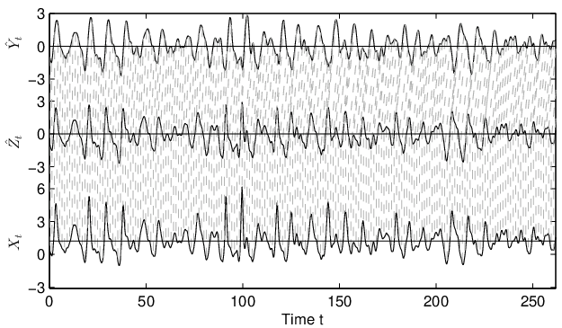
Marine coastal systems are subject to loadings induced by ocean waves and long time series of wave conditions are often needed to study the performances of such systems. It is very difficult to measure wave conditions on long periods of time and thus there is a need for stochastic models which can simulate quickly long time series of wave conditions with realistic characteristics. The systems are often located near the shore where the waves are known to be non-linear. Figure 1 (bottom plot) shows a typical time series of sea-surface elevation in shallow water. It exhibits both different shapes for crests and troughs, with sharp crests and flat troughs, and asymmetries between the steeper front of waves and their backs. Many other situations in environmental science or in econometric lead to study asymmetric records and there is a need for simple and tractable alternatives to Gaussian processes. An approach based on applying a time change to a Gaussian process is investigated in this paper.

A time-changed process is defined as
| (1) |
where denotes a non-decreasing stochastic process referred to as the time change hereafter. is a stochastic process which represents the evolution of the phenomenon of interest in the original time scale. Bold letters are used to stress the fact that and are possibly multivariate processes. is generally referred to as the base process in the literature.
Models with time change have become popular for financial applications since they were introduced in [5] (see e.g. [16] for a recent review). In this application field the modified time is generally interpreted as a ’business time’ and and are generally assumed to be independent Levy processes. Deformations have also been extensively used for modeling non-stationary fields in environmental applications since the seminal paper [13]. It generally consists in seeking a deterministic transformation to map a stationary field into a non-stationary field through (1). These methods can deal with multidimensional (e.g. spatial) fields but they generally require replicates of the random field as input to fit the model. More recently methods that can deal with a unique realization of a densely observed field were proposed (see [1] and references therein). Bayesian approaches where the deformation is modeled using a Gaussian prior were also proposed in [15] and then extended to include covariates in [14].
Specific models which include a time change have already been proposed for modeling wave data. Of particular interest is the two-dimensional stochastic Gauss-Lagrange ocean wave model discussed in [9]. The “space wave” which describes the one-dimensional sea-surface elevation at a fixed time is defined implicitly as
where and denote correlated Gaussian processes which describe respectively the horizontal and vertical motions. Note that the observed process is the sea surface elevation which is a univariate process. In this model the trajectories are defined uniquely and explicitly as (1) only if is one to one which does not always hold true. Another model based on applying a moving average on a Laplace motion (or variance Gamma process) is used in [11] and validated on the same dataset than considered in this paper. A Laplace motion can be defined as (1) with a Brownian motion and an independent Gamma process.
The originality of the model considered in this paper consists in assuming that the time change is a stochastic process which depends on the base process . More precisely, the first model considered in this paper assumes that
| (2) |
with a stationary (ergodic) process and a positive function referred to as the time change function hereafter. In this model the time change is thus a function of the base process and links the speed of the chronometer to the observed process. This model is quite general since can be multivariate and include for example covariates or latent variables. Note that (2) can be rewritten equivalently as
| (3) |
where denotes the reciprocal function of .
Then we consider a more specific model for sea-surface wave elevation where the time change is a deterministic function of the path of the process and its derivative. More precisely we assume that
| (4) |
with a univariate differentiable stationary ergodic Gaussian process, the derivative of and a positive function. A Gaussian process has symmetric paths and (4) will permit to create both crests-troughs or vertical asymmetries (i.e. different shapes for the crests and the troughs) and front-back or horizontal asymmetries (i.e. different shapes for the front and the back of the waves). An example of sequence simulated with this model is shown on Figure 1. The chosen function is increasing in both variables. It implies that the modified time increases quicker when the process is at high levels and thus that the crests of the time modified process are narrower than the ones of with the opposite holding true for the troughs. The chronometers also accelerates with the derivatives of the process and this leads to steeper wave fronts compared to the backs.


The time change impacts the marginal distribution and a process defined by (4) may have non-Gaussian marginal distribution. However the time change does not modify the level of the process and as a consequence the up-crossings of and share similar characteristics. A marginal transformation is then added to add flexibility in the modeling of the up-crossing intensity which is an important quantity for many applications. More precisely we assume that
| (5) |
with defined by (4), the observed process and an increasing function referred to as the marginal link function hereafter.
If then the process defined by (4-5) satisfies with a Gaussian process. This model, which is sometimes referred to as transformed Gaussian model in the literature, is very classical for modeling processes or time series with non-Gaussian marginal distribution and has been extensively used in particular for wave data (see e.g. [12]). Gaussian processes have symmetric paths and this has implications on the paths of a transformed Gaussian process which can handle some crests-troughs asymmetries but no front-back asymmetries. This is a clear limitation of transformed Gaussian models which cannot reproduce wave sequences such as the one shown on Figure 1 which exhibits both kind of asymmetries.
The modeling principle is summarized on Figure 1. Starting from an observed trajectory with asymmetric path (bottom left), we first apply a marginal transformation (5) where the estimated function is shown on the bottom right panel. The concavity of this estimated function leads to decreasing the steepness of the crests compared to the troughs (middle left). Then a time deformation (4) is applied. The estimated function is increasing in both variables (see middle right panel) and thus the chronometer accelerates with the level and the process and its derivatives. It permits to act on both vertical and horizontal asymmetries and obtain a transformed trajectory which has approximatively symmetric path (top left) and can reasonably be modeled using a Gaussian process. The practical motivation for this work was to develop methods to generate quickly long time series of sea-surface elevation with similar characteristics than the observed one. Using one of the methods that have been proposed in the literature to simulate Gaussian processes, realizations of can be quickly generated. It is then easy to deduce realizations of the transformed process once the transformation and have been estimated.
The distribution of the process defined by (4-5) is characterized by the functions and and by the second order structure of the Gaussian process . This paper proposes methods to estimate these functions. For simplicity reasons we first focus on the time change model with no marginal transformation. In Section 2 we consider the general model defined by (2) and give conditions which imply stationarity and ergodicity. This result is then used in Sections 3 and 4 to build respectively parametric and nonparametric estimates of in the model (4). Section 5 discusses the estimation of and and the second order structure of the Gaussian process in the model defined by (4-5). Section 6 discusses the results obtained when fitting this model to a specific wave dataset and conclusions are given in Section 7.
2 Stationarity and ergodicity
In this section we consider the model defined by (3). and , as well as and will denote the processes . The stationarity of means that for any measurable function , has same distribution as for any . The ergodicity means that for any bounded measurable function
In order to check stationarity and ergodicity, it suffices to consider functions of the form
| (6) |
where is a bounded Borel measurable function; we may even assume that is continuous. We will however keep the notation since it will appear to be handier.
Proposition 1.
Let be a stationary process with values on and continuous sample paths and be a measurable real positive function defined on such that . Define the process by (3). Then is stationary for the measure defined as
If is ergodic then is ergodic under . In particular for any measurable real function defined on such that
| (7) |
The proof of this proposition is given in the appendix. (7) is the key result for the rest of this paper. It shows that empirical means computed on a realization of the time changed process converges when the length of the realization tends to infinity. The limit depends both on the distribution of the base process at time and on the time change function .
3 Method of moments
In this section we consider the model defined by (4). It is a particular case of the model defined by (2) with and Proposition 1 gives stationarity and ergodicity conditions for . We further assume that is a Gaussian process and thus for any time the random variables and are independent Gaussian variables. We have and we can assume without loss of generality that . We also assume that and . It is not restrictive in the practical application discussed in Section 6 since this condition will be taken into account when estimating the marginal transformation (see Section 5).
3.1 Moments in the general case
The following proposition gives a general expression for the joint moments of .
Proposition 2.
Let be a univariate differentiable ergodic stationary Gaussian process such that and . Let denote a two dimensional standard normal vector. Assume that (4) holds true with a positive measurable real function such that
| (8) |
Then is a differentiable ergodic stationary process. Let be a measurable real function defined on such that . The stationary measure is such that
| (9) |
Proof.
with . Thus (9) holds true since and are independent variables. ∎
The previous proposition shows that the time change function is related to the joint distribution of and thus suggests estimating to match the empirical joint distribution of . Note however that the relation is not straightforward and that it seems difficult to deduce an estimate of from an estimate of this joint distribution in the general case. Two different simplifications are considered hereafter. In the first one, which is discussed in the rest of this section, we assume a parametric shape for . In the second one, which is discussed in the Section 4, we assume that is product of two functions. This leads to an explicit expression for the joint probability density function (pdf) of and the derivation of nonparametric estimates for .
3.2 Moments in the quadratic exponential model
In the rest of this section we assume that the time change function has a quadratic exponential shape defined as
| (10) |
with unknown parameter . and describe the effect of the level of the base process on the time change and thus the vertical asymmetry whereas and describe the effect of the derivative and the horizontal asymmetry. may be interpreted as an interaction coefficient and as a scale factor. We discuss the realism of this condition for wave data in Section 6. Other parametric time change function may be dealt with in a similar way.
Proposition 3.
Let be a univariate differentiable ergodic stationary Gaussian process such that and . Assume that (4) holds true with given by (10) and that the matrix is definite positive. Then is a differentiable ergodic stationary process. The stationary marginal distribution of is Gaussian with mean and variance such that
| (11) | ||||
| (12) |
Denote , , . Then
| (13) | ||||
| (14) | ||||
| (15) | ||||
| (16) | ||||
| (17) | ||||
| (18) | ||||
| (19) | ||||
Proof.
The model which defines in Proposition 3 is referred to as the quadratic exponential model hereafter.
3.3 Some simulation results in the quadratic exponential model
Various estimates of can be built based on the relations given in Proposition 3. Two possibilities which we have tried are introduced in this section and compared using simulations.
A first estimate, denoted hereafter, can be obtained by solving (14-19) with the theoretical moments replaced by their empirical estimates and estimated using (13). In practice , and are obtained using respectively (14), (15) and (17). Then an expression for is derived from (16) and (18) (note that the term appears in these two formulas). Finally and are estimated using (17) and (19) with the first equation used to express as a linear function of and the second one to give a second order equation for .
Simulation results indicate that provides poor estimations for the parameters and (see Figure 3) which describe the effect of the level of the process on the time change. It suggests using (11-12) to reestimate these parameters using
| (20) | ||||
| (21) |
with the theoretical moments being replaced by their empirical estimates and by in the right hand terms. We denote the corresponding estimates.
Let us now introduce the numerical setup used to perform the simulations. We have chosen to consider parameters values obtained when fitting the model to the wave data shown on Figure 1. The parameters was found to be close to (see Section 6.3 for a more detailed discussion) and it was decided to force this parameter to be equal to . It permits to obtain a model with no interaction which is compatible with the assumptions made in Section 4 and allows comparison between the parametric and the nonparametric approaches. More precisely the chosen parameter values is . The corresponding function is shown on Figure 4 and the spectral density which has been used to simulate the Gaussian process is very close to the one shown on Figure 1. The peak period for is about , the sampling time step is and the length of the simulated sequence is time points. It corresponds to approximatively waves. This is equivalent to a few hours of wave measurements in the ocean and to the length of the measurements described more precisely in Section 6. The simulated sequences have similar characteristics than the sequence shown on Figure 1 (left middle plot) with both crests-troughs and front-back asymmetries.
Figure 3 shows an important improvement in the estimation of and when using and , the other estimates being unchanged by construction. Simulations with other parameter values confirmed these results and led us to keep the estimate hereafter.

4 Non-parametric estimation
In this section we still consider the model defined by (4) with a stationary differentiable ergodic Gaussian process. In order to get an explicit and tractable expression for the joint pdf of and deduce non-parametric estimate of we further assume that there is no interaction between the effect of the level and the derivative, i.e. for any
| (22) |
We discuss the realism of this condition for wave data in Section 6. In this model is related to the vertical asymmetries whereas describes horizontal asymmetries. An increasing function leads to a process with crests narrower than the troughs and if is increasing then the front of the waves are steeper than the back.
The joint pdf of is given in Section 4.1. This result is used in Section 4.2 to build non-parametric estimates of and . A simulation experiment is performed in Section 4.3 to assess the performance of the estimates.
4.1 Joint distribution of in the model with no interaction
Proposition 4.
Let be a univariate differentiable ergodic stationary Gaussian process such that and . Assume that (4) holds true with a positive continuously differentiable real function such that (8) and (22) hold true. Assume further that and are continuously differentiable functions and that the function is one to one and denote its inverse function. The stationary measure is such that for any bounded measurable function
with joint pdf
| (23) |
The model which defines in Proposition 4 is referred to as the model with no interaction hereafter.
4.2 Non-parametric estimation in the model with no interaction
Identifiability constraints. In this section we assume that the conditions of Proposition 4 hold true and discuss the estimation of the functions and . These functions are defined up to a multiplicative constant and hereafter we assume, without loss of generality, that
| (24) |
and thus that .
Marginal and conditional pdf. We then deduce from (23) that the stationary marginal pdf of and conditional pdf given are given respectively by
| (25) | |||
| (26) |
Estimation of .
The estimate of considered hereafter is based on (26) where appears as a scale factor of the conditional distribution of given . More precisely we have and
| (27) |
can be estimated by plugging in a non-parametric estimate of the conditional expectation in this relation. In practice we used the Nadaraya-Watson kernel estimate originally proposed in [10, 17].
An alternative estimate of is suggested by (25) which shows that the marginal distribution of depends only on and not on . More precisely we have
| (28) |
and an estimate of may be obtained by replacing the true pdf by a parametric or non-parametric estimate in this relation. Note however that the unknown constant appears in this relation and thus need to be estimated from the data. A possible estimate of may be obtained using the up-crossing intensity of the zeros level which satisfies (see Section 5 for more details)
This estimation strategy is not further discussed hereafter for simplicity reasons but may be useful in applications where the marginal distribution of (and its tails for example) is of particular importance. We found that both approaches give similar results on simulations and the link between both estimates is further discussed in Section 5 (see (33)).
Estimation of . Let us denote . According to (26) is independent of and the pdf of is
It means in particular that for the model with no interaction the conditional distribution of given depends on the level only through a scale factor . We then deduce that
and thus, after integration between 0 and (note that is increasing and ), we get
and finally
| (29) |
This expression is used to derive the following non-parametric estimate for as described below.
- 1.
Compute where is the estimate of .
- 2.
Estimate using a simple Monte Carlo approach, e.g. for by
where denotes the length of the observed sequence. Plug this estimate in (29) to deduce an estimate of .
- 3.
By definition, is the inverse function of and thus
The next step consists in inverting numerically this relation after replacing by to deduce an estimate of .
- 4.
In practice the estimate is noisy close to the origin (the computation of leads to a division by at the origin) and we found it useful to smooth the estimate close to the origin. In this work the LOESS (locally weighted polynomial regression) smoothing method was used.
4.3 Some simulation results
The performance of the estimates discussed in Section 4.2 was assessed using simulations of the quadratic exponential model with no interaction considered in Section 3.3. Note that for this model we have
and that this function in strictly increasing on if and only if . This condition is satisfied for the parameters values used for the simulations (see Section 3.3). It implies that the function is one to one and thus Proposition 4 applies.
Figure 4 shows typical parametric and non-parametric estimates of obtained on a simulated sequence. Both estimates seem to be able to reproduce the global shape of with the non-parametric estimate being more noisy. Figure 5 shows fluctuation intervals based on simulated sequences and permits a more systematic comparison of both estimates. Again both approaches provide reasonable estimates of and and there is no clear superiority of one of them. The chosen estimation method may thus depend on the application. The parametric estimate is specific to the quadratic exponential model. If this model is not appropriate for a particular application then other parametric model may be developed or the non-parametric approach may be considered. Note however that the non-parametric approach is valid only for the model with no interaction and that this assumption may also be restrictive for some applications. We will see in Section 6 that the quadratic exponential model seems realistic for the particular wave dataset considered in this paper. In such situation the parametric estimate has the additional advantage of providing a description of the observed sequence with a small number of parameters.


5 Model with marginal link function
In this section we discuss the statistical inference in the model defined by (4-5) where a marginal transformation is added to the model discussed in the previous sections. Section 5.1 is devoted to the estimation of the marginal link function . The estimation of the time change function and of the second order structure of the Gaussian process is discussed respectively in Sections 5.2 and 5.3.
5.1 Up-crossing intensity and estimation of
As already mentioned in the introduction, if then the model reduces to with a Gaussian process. This transformed Gaussian model is usual for analyzing wave data and at least two different strategies have been proposed in the literature to estimate . The first one is based on the marginal distribution of which is directly related to , and the second one uses the up-crossing intensity (see [12, 2] and references therein).
Both approaches may be extended to the model defined by (4-5). However the marginal distribution of depends on both and and it leads to complicated estimation procedures when trying to isolate the effect of on this distribution. We have thus chosen to focus on methods based on up-crossings. Indeed the time deformation does not modify the levels of the observed sequence and thus the up-crossing intensity will mainly depend on (up to a normalizing constant). This is stated more formally in the proposition below.
Proposition 5.
Let be a univariate differentiable ergodic stationary Gaussian process such that and . Assume that (4-5) hold true with a positive measurable real function such that (8) holds true and an increasing function. Let denotes the number of up-crossings of the level of the process on the time interval and the up-crossing intensity. Then
| (30) |
Proof.
Since is increasing and the time change does not modify the observed level we have . We deduce that
The previous proposition has been used to build non-parametric estimates of as described below. According to (30) we get
| (31) |
needs then to be estimated from the data in order to be able to use this relation to estimate . For that we used that
| (32) |
which shows that can be estimated from the mode of the up-crossing intensity (ie the intensity of the most often crossed level). Once is estimated we are faced to a similar estimation problem than discussed in [12] for transformed Gaussian models. It consists in taking a square root of (31) using the monotony of and eventually smoothing the obtained estimates (the loess method was used in this work). An isotonic regression method may also be applied to force the obtained estimates to be increasing but this was not necessary for the practical cases considered in this paper.
Figure 6 shows simulation results obtained with the setting described in Section 3.3 and estimated from the data (the true function used for the simulations is shown as a full line on the left plot). The bias and variance of the estimate are generally low with higher variances in the tails where the number of up-crossings is lower. Note also that the concavity of implies that the marginal distribution of has a fatter upper tail compared to the lower tail and this has consequences on the estimate of which has a higher variance in the upper tail.
5.2 Estimation of
The estimation of when the process is observed has been discussed in the previous sections. However only is generally observed when considering the model (4-5). Once is estimated it is possible to compute an approximation of as
with the estimate of . Estimates of the time change function can then be obtained by replacing the latent process by in the methods described in Sections 3 and 4. Comparing the right plots of Figures 6 and 3 shows that using instead of modifies the statistical properties of the estimates of in the parametric case (similar results were obtained with the non-parametric estimates introduced in Section 4). It is not surprising since is estimated such that the up-crossing intensity of has a Gaussian shape (see (30)) and this up-crossing intensity is related to the joint distribution of via the Rice formula as follows
Estimates of are based on this joint distribution and thus may be impacted when using instead of . Note also that this relation implies that
| (33) |
and may explain why the non-parametric estimates of based on (28) or (27) lead to similar results (it can be shown that a similar relation holds true when replacing and by non-parametric kernel estimates).

5.3 Estimation of the second order structure of
is stationary Gaussian process with zero mean and is thus completely characterized by its second order structure. Again the process is not directly observed but can be approximated when the function and have been estimated. In order to simplify the presentation we assume in this section that the process is observed. In the practical applications it is not observed but replaced by the approximation introduced in the previous section. Recall that the time change is defined through the following differential equation
| (34) |
with and related to implicitly as follows
| (35) |
A Euler scheme has then been used to compute an approximation of defined by (34) where the implicit equation (35) is solved at each time step. In the separable model defined in Section 4 it can be easily done using
and the function is directly estimated from the data. A numerical optimization procedure was used to solve (35) in the quadratic exponential model.
We can then deduce an approximation of and compute a standard estimate of the second order structure (autocorrelation or spectral density) on the sample .
6 Application to wave data
This section starts with a brief overview of physically based wave models which lead to time or space deformations. We then introduce the wave dataset and discuss the results obtained when fitting the model (4-5) to this dataset.
6.1 Physical motivations
In the gravity wave theory the non-linear solution of the free surface evolution has been proven to be well approximated by the first order linear Lagrangian solution of the Euler equations (Gerstner wave in harmonic case, Pierson ([7]) for multi-harmonic or irregular waves).) Let denote the two-dimensional linear trajectory of a water particle of the free surface located in at time , such that the height of the water surface at time and location is . The non-linear (Eulerian) free surface elevation is thus given by
It corresponds to a modulation in space of the vertical movements of the particles. In the case where the modulation is strong the solution of this implicit equation may not be unique. It corresponds in the physical meaning to wave breaking.
More recently a canonical Lie transformation was proposed for gravity waves in order to transform the real physical world in a linear (more exactly close to linear) world or inversely (see [6]). In the infinite water depth case it leads to an Inviscid Burgers’ equation on the free surface elevation
with and the Hilbert transform in space. and correspond to respectively the free surface elevation in the linear and non-linear worlds. The solution of the Burgers’ equation satisfies
Again modulation of space appears as a natural way to transform linear waves to non-linear ones. In the case of finite water depth and of more complex situations with varying sea bottom in shallow water, the solution of the Euler equations are not so simple, but the idea of modulation by a function of the process itself could appear still pertinent.
6.2 Data
The proposed methodology was used to analyze wave data from an experiment carried out in a wave flume. A detailed description of the experiment can be found in [4]. The bathymetric profile of the flume experiment is shown on Figure 7 together with the various locations where the sea-surface elevation is measured (numbered from 1 close to the wave-maker to 16). The wave-maker generates random phase waves which are expected to be close to a realization of a Gaussian process with a JONSWAP-type spectra. Then the waves propagate to the right on a varying bathymetry which induces strong non-linearities. Examples of time series measured at locations and are shown on Figure 7. It shows in particular that both horizontal and vertical asymmetries increase when the waves propagate to the right. Free surface elevation is recorded over a duration of 40 minutes with a sampling time-step of . The peak period is about . It corresponds to about 1000 waves with 34 points per wave.


6.3 Results
The model (4-5) was fitted at the locations where wave measurements are available but in the discussion below we mainly focus on the central location . According to Figure 8 the parametric approach for the quadratic exponential model and the non-parametric approach for the model with no interaction lead to estimates with similar shapes for at location . It is a first indication that the choice of the quadratic exponential model is sensible for the wave dataset considered in this paper. Both the parametric and non-parametric approaches were validated using the criteria discussed below and generally slightly better results were obtained with the parametric approach. We have thus chosen to focus on this approach hereafter. It has the additional advantage of providing a parsimonious description of the observed sequence with only parameters involved. Figure 9 shows the evolution of the estimates with the measurement location. At locations and , where it is expected that the observed sequences may be modeled as a realization of a Gaussian process, low estimated values are obtained for all the parameters except the intercept . It corresponds to an almost constant time change function as in the Gaussian case. Then from location the parameters values evolve with the varying bathymetry. This evolution is relatively smooth in space. This could be used for example to interpolate the parameter values and simulate synthetic waves at locations with no observation. Note that parametric models such as power transformations and classical wave spectral models may also be considered for and the spectrum of to get a full parametric model.
According to Figure 9 the values of the interaction term is always low and this suggests that a model with no interaction () may be appropriate. Fluctuation intervals for the estimates can be computed using similar simulations as in Section 5.2. The 95% interval obtained for at location is . It suggests that the interaction term is low but still statistically significant.


Let us now focus on location and validate the fitted quadratic exponential model. Figure 1 shows the estimates of , and the spectral density of at location . As already mentioned in the introduction the estimated function is increasing in both variables and this permits to create both vertical and horizontal asymmetries by accelerating the chronometer in the crests and in the front of the waves. is concave and thus enhance again the sharpness of the crests by boosting high levels. If the fitted model is appropriate then the marginally and time transformed sequence should have paths which can be reasonably modeled as a realization of a Gaussian process. No formal test was performed but Figure 1 shows a sequence of this process and that the marginal and time transformations permit to symmetrize the path of the observed sequence. Another way to validate the model consists in generating sequences of the fitted model and compare the statistical properties of the simulated sequences with the ones of the original data. We focus on this validation strategy hereafter since it is directly related to the practical application (we want a model which can generate realistic wave sequences) and it is also probably easier to interpret than validation in the Gaussian domain. Note that the fitted model can be very quickly simulated (about one half second to generate 1000 waves on a basic laptop using Matlab).


An example of simulated sequence is shown on Figure 10. It looks visually coherent with the observed sequence shown on the same figure. A more systematic comparison is performed below. Figure 11 shows the marginal and joint pdf of . This distribution is relatively complex with an asymmetric distribution for (the empirical skewness of is ), a leptokurtic marginal distribution for (the empirical skewness of is ) and a complex relation between both variables with for example higher steepness in the crests. The fitted model is able to reproduce the complexity of this distribution. The marginal distribution of is of particular importance for the applications and the quantile-quantile plot shown on Figure 12 confirms that the fit is good except maybe in the upper tail where the fit is slightly less good. An appropriate parametric model for the tails of may be useful here.
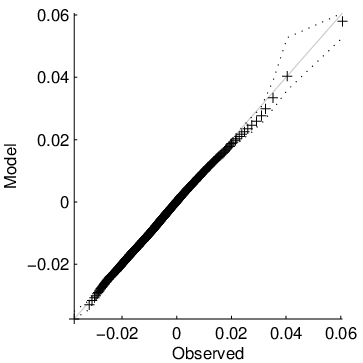


Figure 12 also shows that the second order structure of the data is well reproduced by the fitted model except the third peak in the observed spectrum. This third peak is induced by non linear effect which create a low amplitude high frequency components which phase is linked to the other frequencies. The fitted model is not able to reproduce this non-linear interaction but still reproduces the associated asymmetries. Indeed Figure 13 shows the distribution of the various slopes (crest front, crest back, trough front, trough back) computed after extracting individual waves using zeros-crossings (see [11] for a more precise definition and [3] for a review of existing measures of asymmetries). The differences in these four distributions are linked to the asymmetries in the sea surface elevation. For example it shows that the fronts of the crests are the steepest whereas the fronts of the troughs are the flattest. These slope distributions are well reproduced by the fitted model.
7 Conclusions and perspectives
This paper proposes a new model for asymmetric time sequences. The originality of the proposed model consists in introducing a time change which is dependent of the observed process. The proposed statistical inference is based on the up-crossings and on the joint distribution of the process and its derivatives. Simplifying assumptions are imposed on the shape of the time change function in order to be able to derive estimates for . We show that these assumptions seems realistic for the particular wave dataset considered in this paper but it may be useful to consider other cases for other applications. This remains to be further investigated together with other modeling issues such as the extension to a spatial or space-time context.
Appendix : proof of Proposition 1
Proof.
. Let us denote the shifted processes and the processes obtained by replacing is replaced with in (3). We get
It can then be deduced that which means that the effect of a shift on is a random shift on .
Now, by the stationarity of , we have for any and any function of the form (6)
Hence, for any
and for any
Since the right hand side can be made arbitrarily small, we have proven the stationarity. Similar equations can be used for proving the ergodicity. Indeed we have
| (36) |
where denotes the reciprocal function of . Note that
by the ergodicity of and thus . Using again the ergodicity of and that
we deduce that the second term in the right hand size term of (36) converges to a deterministic limit which is its expected value.
(7) is a particular case of the general convergence result proved above with and remarking that .
∎
References
- [1] E. B. Anderes and M. L. Stein. Estimating deformations of isotropic gaussian random fields on the plane. The Annals of Statistics, pages 719–741, 2008.
- [2] J.-M. Azaïs and M. Wschebor. Level sets and extrema of random processes and fields. John Wiley & Sons, 2009.
- [3] A. Baxevani, K. Podgórski, and J. Wegener. Sample path asymmetries in non-gaussian random processes. Scandinavian Journal of Statistics, 41(4):1102–1123, 2014.
- [4] F. Becq-Girard, P. Forget, and M. Benoit. Non-linear propagation of unidirectional wave fields over varying topography. Coastal Engineering, 38(2):91–113, 1999.
- [5] P.K. Clark. A subordinated stochastic process model with finite variance for speculative prices. Econometrica: journal of the Econometric Society, pages 135–155, 1973.
- [6] D. B Creamer, F. Henyey, R. Schult, and J. Wright. Improved linear representation of ocean surface waves. Journal of Fluid Mechanics, 205:135–161, 1989.
- [7] Pierson W.J. Jr. Models of random seas based on the lagrangian equations of motion. Technical report, Technical report, College of Engineering, Research Division, New York University., 1961.
- [8] G. Lindgren. Lectures on stationary stochastic processes. Lecture Notes, Lund University, 2006.
- [9] G. Lindgren. Exact asymmetric slope distributions in stochastic gauss–lagrange ocean waves. Applied Ocean Research, 31(1):65–73, 2009.
- [10] E.A. Nadaraya. On estimating regression. Theory of Probability & Its Applications, 9(1):141–142, 1964.
- [11] N. Raillard, M. Prevosto, and P. Ailliot. Modeling process asymmetries with Laplace moving average. Computational Statistics & Data Analysis, 81:24–37, 2015.
- [12] I. Rychlik, P. Johannesson, and M.R. Leadbetter. Modelling and statistical analysis of ocean-wave data using transformed gaussian processes. Marine Structures, 10(1):13–47, 1997.
- [13] P.D. Sampson and P. Guttorp. Nonparametric estimation of nonstationary spatial covariance structure. Journal of the American Statistical Association, 87(417):108–119, 1992.
- [14] A.M. Schmidt, P. Guttorp, and A. O’Hagan. Considering covariates in the covariance structure of spatial processes. Environmetrics, 22(4):487–500, 2011.
- [15] A.M. Schmidt and A. O’Hagan. Bayesian inference for non-stationary spatial covariance structure via spatial deformations. Journal of the Royal Statistical Society: Series B (Statistical Methodology), 65(3):743–758, 2003.
- [16] A.E.D. Veraart and M. Winkel. Time change. Encyclopedia of quantitative finance, 2010.
- [17] G.S. Watson. Smooth regression analysis. Sankhyā: The Indian Journal of Statistics, Series A, pages 359–372, 1964.