The top quark right coupling in the tbW-vertex

Top properties were studied in previous works by means of the observables that we just mentioned. One of the first possibilities are the angular asymmetries for the $t\rightarrow W^{+}\,b$ decay, with the $W^{+}$ decaying leptonicaly. The normalized charged lepton angular distribution in the W rest frame can be written as:

where $F_{0},F_{\pm}$ are the normalized partial widths of the top decay into the W helicity states, and $\theta_{l}$ is the angle between the charged lepton momentum in the $W$ rest frame and the $W$ momentum in the $t$ rest frame. Then, the asymmetries are defined, in terms of a new parameter $z$, as follows [21, 10]:

The $z$ parameter allows to separate the helicity fractions $F_{0},F_{\pm}$. The value $z=0$ gives the usual forward-backwards asymmetry while $z=\pm(2^{2/3}-1)$ defines the $A_{\mp}$ asymmetries, respectively. The first one, $A_{0}$ depends only on the $F_{\pm}$ helicity fractions while $A_{\pm}$ depends on both $F_{0}$ and $F_{\pm}$.

The helicity fractions, $F_{0}$ and $F_{\pm}$, can be computed in terms of the $tbW$ couplings given in eq. (1), and they can be found, for example, in ref. [22]. Performing the $\theta_{l}$ integration of eq. (6) for a given value of $z$, the numerator of the asymmetry $A_{z}$, in terms of $V_{L}$ and $V_{R}$ is:

One can now choose the value of the $z$ parameter, within the range $(-1,1)$, to make zero the leading $V_{L}$ contribution. In this way we get the maximum sensitivity to $V_{R}$. The coefficient of $V_{L}^{2}$ and $V_{R}^{2}$ from eq. (7), are plotted in figure 3.

There, it can be seen that for $z=\displaystyle z_{R}=-0.17$ the coefficient of $V_{L}^{2}$ cancels, leaving the $V_{R}$ term, in eq. (7), as the leading one. For this $z_{R}$ the new asymmetry $A_{R}\equiv A_{Z}(z=z_{R})$ is proportional to $V_{R}$ and has the form:

where the last expression is the value of the asymmetry taking $V_{L}=1$ and assuming $|V_{R}|<<1$. As can be seen this asymmetry is directly proportional to $V_{R}$ so that a non-zero measurement of it is a direct test of $V_{R}\neq 0$.

Note that the leading contribution to the usual $A_{\pm}$ asymmetries comes from $V_{L}^{2}$ so that in order to be sensitive to $V_{R}$ one needs to subtract this SM central value. In figure 3 we show the $V_{R}$ dependence of $A_{R}$ and also, for comparison, the dependence of $A_{\pm}$, with the $V_{L}^{2}$ leading contribution subtracted. As can be seen there $A_{R}$ may allow more precise bounds on $V_{R}$. Besides, it is directly proportional to $V_{R}$ and eliminates other uncertainties that the $V_{L}$ dependence in $A_{\pm}$ may introduce.

For polarized top it is possible to define asymmetries with respect to the normal and transverse spin directions. These were studied in ref. [11], but they are not sensitive to the $V_{R}$ coupling so we are not going to consider them in our analysis.

Angular distribution of the decay products for the weak process $t\rightarrow W^{+}b$ carries information about the spin of the decaying top. Then, angular asymmetries can be built to test the Lorentz structure of the vertex. We will follow the same procedures described previously, in order to optimize the sensitivity of the observables to $V_{R}$ but, in this case, for the asymmetries in the top rest frame.

For the top decay $t\rightarrow W^{+}\,b\rightarrow l^{+}\nu b,q\bar{q}^{\prime}b$, the angular distribution of the product $X=l^{+},\nu,q,\bar{q}^{\prime},W^{+},b$, in the top rest frame, is given by:

where $\theta_{X}$ is the angle between the momentum of $X$ and the top spin direction, and $\alpha_{X}$ are the spin-analyzer powers, given in references [22, 23, 29, 24, 11] in terms of the couplings shown in eq. (1). Then, an asymmetry can be defined as:

For $z=0$, one gets the usual forward-backward asymmetry:

Sensitivity to $V_{R}$ and $V_{L}$ for this asymmetry have already been given for $X=l^{+},\;b,\;\nu$ in the $t$-channel single top production in refs. [30, 11]. In order to define a new asymmetry directly proportional to the $V_{R}$ coupling one can again extract the SM leading contribution, given by the $V_{L}^{2}$ term in the $A_{X}^{z}$ asymmetry, and make it zero. For the $X=$ $l$, $\nu$, $b$ cases, the eq. (10) is:

Figure 5 shows the behavior of the $V_{L}^{2}$ coefficient from the $A_{l}$, $A_{b}$ and $A_{\nu}$ asymmetries. We can choose $z$ in order to make the leading coefficients of eqs. (12), (13) and (14) to be zero. These $z$ values are:

and then, the new asymmetries are:

where in the last expression we show the value of the asymmetries for $V_{L}=1$ and assuming $|V_{R}|<<1$. From eq. (12) one can see that unfortunately, for the $A_{l}$ asymmetry, the same value of $z$ that cancels the coefficient of $V_{L}^{2}$ also cancels the $V_{L}V_{R}$ term, in such a way that a poorer sensitivity to the coupling will be expected from this observable because the surviving term is $V_{R}^{2}$ instead of $V_{L}V_{R}$.

In figures 5, 7 and 7 we show the dependence on $V_{R}$ for the new $A_{l}^{z_{l}}$, $A_{b}^{z_{b}}$ and $A_{\nu}^{z_{\nu}}$ observables. We have explicitly checked that the usual forward-backward asymmetries for the same decay product have a very similar behavior as the ones shown in the figures, once the leading $V_{L}^{2}$ contribution is removed. However, the new observables again have the advantage that are proportional to $V_{R}$ so that their measurement may provide a direct bound or measurement of the $V_{R}$ coupling with no assumption on the value of the $V_{L}^{2}$ leading term.

The top–antitop spin correlations depend on the Lorentz structure of the $tbW$ vertex. This structure can be studied through the measurement of the angular distributions of the decay products for the $t\rightarrow W^{+}b$ and $\bar{t}\rightarrow W^{-}\bar{b}$ processes, that carry information on the top and antitop spin correlation terms. In particular, using the notation of previous section, the double angular distribution – of the decay products $X$, from top, and $\bar{X}^{\prime}$, from antitop – can be written as [26, 25]:

where $\theta_{X}$ ($\theta_{\bar{X}^{\prime}}$) is the angle between the momentum of the decay product $X$ ($\bar{X}^{\prime}$) and the momentum of the top (antitop) quark in the $t\bar{t}$ center-of-mass frame, $\alpha_{X}$ and $\alpha_{\bar{X}^{\prime}}$ are the spin analyzer powers of particles $X$ and $\bar{X}^{\prime}$, respectively. $C$ is a coefficient that weights the spin correlation between the quark and the antiquark. Then, one can define the asymmetry

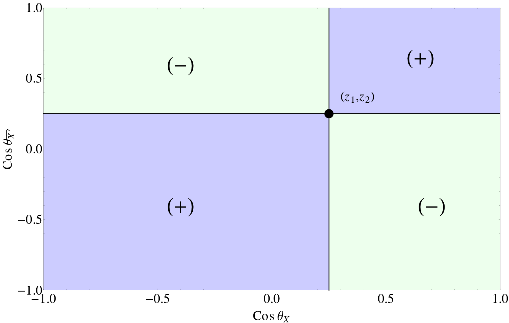
The different regions of integration for this asymmetry are plotted in figure 9. There, the number of events on each of the regions is collected and the sign of their contribution to the asymmetry is also indicated. The particular case $z_{1}=z_{2}=0$ corresponds to the usual spin correlation asymmetry:

For the $A_{X\bar{X}^{\prime}}^{z_{1}z_{2}}$ asymmetry, eq. (20), there is a range of values of $z_{1}$ and $z_{2}$ that cancel the leading $V_{L}^{4}$ contribution, in such a way that the observable becomes proportional to the $V_{R}$ coupling. For the $X=l$, $\bar{X}^{\prime}=l^{\prime}$ case, these values satisfy the relation:

Similarly to what happened for $A_{l}^{z}$, in eq. (12), for values of $z_{1}$ and $z_{2}$ satisfying the previous equation, the coefficient of $V_{L}^{3}V_{R}$ in the asymmetry also accidentally cancels. Then, it remains the $V_{R}^{2}$ coupling as the leading contribution. Solutions to eq. (22) are plotted in figure 9 where it can be seen that the values of $z_{1}$ and $z_{2}$ are restricted to be in the first quadrant (for the $z_{2}^{+}$ solution) or in the third one (for the $z_{1}^{-}$ solution). In addition to the trivial solutions of eq. (22), i.e. $z_{1}=\pm 1,z_{2}=0$, that reproduces the usual $A_{ll^{\prime}}$ asymmetry, one can improve the computation by finding the values of $z_{1}$ and $z_{2}$ that, satisfying eq. (22), also maximize the coefficient of the leading $V_{R}^{2}$ term in eq.(20), namely:

This can be trivially done and the result is

that correspond to the intersection of the curves of figure 9 with the diagonal line of the first and third quadrants.

These values of $z_{1}$, $z_{2}$ give a maximum sensitivity of the $A_{ll^{\prime}}^{z_{1}z_{2}}$ asymmetry to the $V_{R}$ coupling.

In figure 11 we show the dependence on the $V_{R}$ coupling for the $A_{ll^{\prime}}^{z_{1}z_{2}}$ asymmetry in eq. (20), for $C=0.4$ [11] , and $z_{1}=z_{2}=z_{ll^{\prime}}=0.29$, given by eq. (24).

The same procedure followed here can be used for other decay products of the $W^{\pm}$. For $t\bar{t}\rightarrow l\,\nu\,b\,\bar{\nu}\,l^{\prime}\,\bar{b}$ final state, the values of $z_{1}$ and $z_{2}$ that cancels the coefficient of the leading $V_{L}^{4}$ term in the $A_{\nu l^{\prime}}^{z_{1}z_{2}}$ asymmetry ($X=\nu$, $\bar{X}^{\prime}=l^{\prime}$ in eq. (20)), satisfy a quadratic equation

and the solution is

Here, $-1\leq z_{1}\leq 0$ for the $z_{2}^{+}$ solution and $0\leq z_{1}\leq 1$ for the $z_{2}^{-}$ solution of eq. (26), in order to satisfy $|z_{2}^{\pm}|<1$. In that case, these set of $z_{1,2}$ values do not cancel the $V_{R}$ term of the asymmetry, that remains as the leading one:

One can easily find the values that maximize this coefficient and simultaneously verify eq. (26):

In figure 11 we show the dependence of the spin correlation asymmetry $A_{\nu l^{\prime}}^{z_{\nu l^{\prime}}z_{\nu l^{\prime}}}$ on $V_{R}$, for $z_{1}$, $z_{2}$ given by eq. (28) with $C=0.4$. Note that the sensitivity of both asymmetries shown in figures 11 and 11 is rather similar.

Another spin correlation considered in the literature is the angular distribution of the top (antitop) decay products defined as [31]:

where $\varphi_{X\bar{X}^{\prime}}$ is the angle between the momentum of the $X$ particle in the $t$ rest frame, and that of the $X^{\prime}$ one, in the $\bar{t}$ rest frame. D is the spin correlation coefficient. Then, one can construct the following asymmetry:

For $z=0$ one gets the usual forward-backward spin correlation asymmetry

For both $W^{\pm}$ leptonic decays, $X=l$ and $\bar{X}^{\prime}=l^{\prime}$, and following similar procedures as in the previous sections, we can find the value of $z$ that cancels the $V_{L}^{4}$ leading term in eq. (30):

This value also cancels the $V_{R}$ term so that the $V_{R}^{2}$ contribution is the dominant one. Then, for $D=-0.29$ [11], the $\tilde{A}_{ll^{\prime}}^{z}$ asymmetry is:

where again, in the last term, we show the asymmetry for $V_{L}=1$ and $|V_{R}|<<1$. This asymmetry can be seen in figure 13.

Analogously, for $W$ leptonic decays with neutrino-lepton final state, $X=\nu$, $\bar{X}^{\prime}=l^{\prime}$, the $z$-value that cancels the $V_{L}^{4}$ term in eq. (30) is

and then, the $\tilde{A}_{\nu l^{\prime}}^{z}$ asymmetry, for $D=-0.29$, is:

The last term in this equation is given for $V_{L}=1$ and $|V_{R}|<<1$. This asymmetry is depicted in figure 13. Note that in this case the sensitivity to $V_{R}$ is lower than the one obtained in some of the previous observables due to the small coefficients in the numerator of eq. (35).

We checked that the expressions of the observables defined for the $V_{R}$ coupling in this section show a behavior comparable to the one obtained from the expressions of the observables defined in the literature, once the $V_{L}$ leading contribution is removed. Moreover, the observables defined here have the advantage of being directly proportional to the $V_{R}$ term that we want to test.

References

- [1] F.-P. Schilling, Top Quark Physics at the LHC: A Review of the First Two Years, Int. J. Mod. Phys. A27 (2012) 1230016, [arXiv:1206.4484].
- [2] R. Hawkings, Top quark physics at the LHC, Comptes Rendus Physique 16 (2015) 424–434.
- [3] W. Bernreuther, Top quark physics at the LHC, J. Phys. G 35 (2008) 083001, [arXiv:0805.1333].
- [4] CDF Collaboration Collaboration, F. Abe et al., Observation of top quark production in collisions, Phys. Rev. Lett. 74 (1995) 2626–2631, [hep-ex/9503002].
- [5] D0 Collaboration Collaboration, S. Abachi et al., Observation of the top quark, Phys. Rev. Lett. 74 (1995) 2632–2637, [hep-ex/9503003].
- [6] C. Deterre, helicity and constraints on the vertex at the Tevatron, Nuovo Cim. C035N3 (2012) 125–129, [arXiv:1203.6802].
- [7] D0 Collaboration Collaboration, V. M. Abazov et al., Search for anomalous couplings in single top quark production in collisions at TeV, Phys. Lett. B 708 (2012) 21–26, [arXiv:1110.4592].
- [8] D0 Collaboration, V. M. Abazov et al., Search for anomalous Wtb couplings in single top quark production, Phys. Rev. Lett. 101 (2008) 221801, [arXiv:0807.1692].
- [9] C. Bernardo, N. F. Castro, M. C. N. Fiolhais, H. Gonçalves, A. G. C. Guerra, M. Oliveira, and A. Onofre, Studying the vertex structure using recent LHC results, Phys. Rev. D90 (2014), no. 11 113007, [arXiv:1408.7063].
- [10] F. del Aguila and J. Aguilar-Saavedra, Precise determination of the Wtb couplings at CERN LHC, Phys.Rev. D67 (2003) 014009, [hep-ph/0208171].
- [11] J. Aguilar-Saavedra and J. Bernabéu, W polarisation beyond helicity fractions in top quark decays, Nucl. Phys. B 840 (2010) 349–378, [arXiv:1005.5382].
- [12] J. Drobnak, S. Fajfer, and J. F. Kamenik, New physics in decay at next-to-leading order in QCD, Phys. Rev. D82 (2010) 114008, [arXiv:1010.2402].
- [13] S. D. Rindani and P. Sharma, Probing anomalous tbW couplings in single-top production using top polarization at the Large Hadron Collider, JHEP 1111 (2011) 082, [arXiv:1107.2597].
- [14] Q.-H. Cao, B. Yan, J.-H. Yu, and C. Zhang, A General Analysis of anomalous Couplings, arXiv:1504.0378.
- [15] A. V. Prasath, R. M. Godbole, and S. D. Rindani, Longitudinal top polarisation measurement and anomalous coupling, Eur. Phys. J. C75 (2015), no. 9 402, [arXiv:1405.1264].
- [16] Particle Data Group Collaboration, K. Olive et al., Review of Particle Physics, Chin.Phys. C38 (2014) 090001.
- [17] M. Moreno Llácer, Search for CP violation in single top quark events with the ATLAS detector at LHC. PhD thesis, Valencia U., IFIC, 2014.
- [18] G. A. González-Sprinberg, R. Martinez, and J. Vidal, Top quark tensor couplings, JHEP 07 (2011) 094, [arXiv:1105.5601]. [Erratum: JHEP05,117(2013)].
- [19] L. Duarte, G. A. González-Sprinberg, and J. Vidal, Top quark anomalous tensor couplings in the two-Higgs-doublet models, JHEP 1311 (2013) 114, [arXiv:1308.3652].
- [20] W. Bernreuther, P. Gonzalez, and M. Wiebusch, The Top Quark Decay Vertex in Standard Model Extensions, Eur. Phys. J. C 60 (2009) 197–211, [arXiv:0812.1643].
- [21] B. Lampe, Forward - backward asymmetry in top quark semileptonic decay, Nucl.Phys. B454 (1995) 506–526.
- [22] J. Aguilar-Saavedra, J. Carvalho, N. F. Castro, F. Veloso, and A. Onofre, Probing anomalous Wtb couplings in top pair decays, Eur.Phys.J. C50 (2007) 519–533, [hep-ph/0605190].
- [23] B. Grzadkowski and Z. Hioki, New hints for testing anomalous top quark interactions at future linear colliders, Phys.Lett. B476 (2000) 87–94, [hep-ph/9911505].
- [24] R. M. Godbole, S. D. Rindani, and R. K. Singh, Lepton distribution as a probe of new physics in production and decay of the t quark and its polarization, JHEP 0612 (2006) 021, [hep-ph/0605100].
- [25] T. Stelzer and S. Willenbrock, Spin correlation in top quark production at hadron colliders, Phys.Lett. B374 (1996) 169–172, [hep-ph/9512292].
- [26] G. Mahlon and S. J. Parke, Angular correlations in top quark pair production and decay at hadron colliders, Phys.Rev. D53 (1996) 4886–4896, [hep-ph/9512264].
- [27] J. Bernabéu, G. González-Sprinberg, and J. Vidal, Normal and transverse single tau polarization at the Z peak, Phys. Lett. B 326 (1994) 168–174.
- [28] J. Bernabeu, G. González-Sprinberg, M. Tung, and J. Vidal, The Tau weak magnetic dipole moment, Nucl.Phys. B436 (1995) 474–486, [hep-ph/9411289].
- [29] B. Grzadkowski and Z. Hioki, Decoupling of anomalous top decay vertices in angular distribution of secondary particles, Phys.Lett. B557 (2003) 55–59, [hep-ph/0208079].
- [30] J. Aguilar-Saavedra, J. Carvalho, N. Castro, M. Fiolhais, A. Onofre, et al., Study of ATLAS sensitivity to asymmetries in single top events, Nuovo Cim. B123 (2008) 1323–1324.
- [31] W. Bernreuther, A. Brandenburg, Z. Si, and P. Uwer, Top quark pair production and decay at hadron colliders, Nucl.Phys. B690 (2004) 81–137, [hep-ph/0403035].