跳到论文正文
W Papers独立论文阅读器 arXiv:1510.01550 论文正文 计算阅读时间 · 0%
引用这篇论文根据当前论文元数据生成,正式投稿前建议核对。


License: arXiv.org perpetual non-exclusive license
arXiv:1510.01550v1 [math.AP] 06 Oct 2015

An analytical and numerical study of steady patches in the disc

, Francisco de la Hoz Address:  Department of Applied Mathematics and Statistics and Operations Research, Faculty of Science and Technology
University of the Basque Country UPV/EHU, Barrio Sarriena S/N
48940 Leioa, Spain
Email address: francisco.delahoz@ehu.eus
, ZINEB HASSAINIA Address: The Courant Institute for Mathematical Sciences, New York University
251 Mercer Street New York, N.Y. 10012-1185
Email address: zineb.hassainia@cims.nyu.edu
, Taoufik Hmidi Address: IRMAR, Université de Rennes 1
Campus de Beaulieu
35 042 Rennes cedex
France
Email address: thmidi@univ-rennes1.fr
and Joan Mateu Address: Departament de Matemàtiques
Universitat Autònoma de Barcelona
08193 Bellaterra, Barcelona, Catalonia
Email address: mateu@mat.uab.cat
Abstract.

In this paper, we prove the existence of mm-fold rotating patches for the Euler equations in the disc, for both simply-connected and doubly-connected cases. Compared to the planar case, the rigid boundary introduces rich dynamics for the lowest symmetries m=1m=1 and m=2m=2. We also discuss some numerical experiments highlighting the interaction between the boundary of the patch and the rigid one.

1. Introduction

In this paper, we shall discuss some aspects of the vortex motion for the Euler system in the unit disc 𝔻\mathbb{D} of the Euclidean space ℝ2\mathbb{R}^{2}. That system is described by the following equations:

(1) {∂tv+v⋅∇v+∇p=0,(t,x)∈ℝ+×𝔻,div​v=0,v⋅ν=0,on∂𝔻,v|t=0=v0.\begin{cases}\partial_{t}v+v\cdot\nabla v+\nabla p=0,\quad(t,x)\in\mathbb{R}_{+}\times\mathbb{D},\\ \textnormal{div}\,v=0,\\ v\cdot\nu=0,\quad\textnormal{on}\quad\partial\mathbb{D},\\ v_{|t=0}=v_{0}.\end{cases}

Here, v=(v1,v2)v=(v^{1},v^{2}) is the velocity field, and the pressure pp is a scalar potential that can be related to the velocity using the incompressibility condition. The boundary equation means that there is no matter flow through the rigid boundary ∂𝔻=𝕋\partial\mathbb{D}=\mathbb{T}; the vector ν\nu is the outer unitary vector orthogonal to the boundary. The main feature of two-dimensional flows is that they can be illustrated through their vorticity structure; this can be identified with the scalar function ω=∂1v2−∂2v1\omega=\partial_{1}v_{2}-\partial_{2}v_{1}, and its evolution is governed by the nonlinear transport equation:

(2) ∂tω+v⋅∇ω=0.\partial_{t}\omega+v\cdot\nabla\,\omega=0.

To recover the velocity from the vorticity, we use the stream function Ψ\Psi, which is defined as the unique solution of the Dirichlet problem on the unit disc:

{Δ​Ψ=ω,ψ|∂𝔻=0.\begin{cases}\Delta\Psi=\omega,\cr\psi|_{\partial\mathbb{D}}=0.\end{cases}

Therefore, the velocity is given by

v=∇⟂Ψ,∇⟂=(−∂2,∂1).v=\nabla^{\perp}\Psi,\quad\nabla^{\perp}=(-\partial_{2},\partial_{1}).

By using the Green function of the unit disc, we get the expression

(3) Ψ⁡(z)=14​π​∫𝔻log⁡|z−ξ1−z​ξ¯|2​ω​(ξ)​𝑑A​(ξ),\Psi(z)=\frac{1}{4\pi}\int_{\mathbb{D}}\log\Big|\frac{z-\xi}{1-z\overline{\xi}}\Big|^{2}\omega(\xi)dA(\xi),

with d​AdA being the planar Lebesgue measure. In what follows, we shall identify the Euclidean and the complex planes; so the velocity field is identified with the complex function

v⁡(z)=v1​(x1,x2)+i​v2​(x1,x2),withz=x1+i​x2.v(z)=v_{1}(x_{1},x_{2})+i\,v_{2}(x_{1},x_{2}),\quad\hbox{with}\quad z=x_{1}+ix_{2}.

Therefore, we get the compact formula

(4) v⁡(t,z)\displaystyle v(t,z) =2​i​∂z¯Ψ⁡(t,z)\displaystyle=2i\,\partial_{\overline{z}}\,\Psi(t,z)
(5) =i2​π​∫𝔻|ξ|2−1(z¯−ξ¯)​(ξ​z¯−1)​ω​(t,ξ)​𝑑A​(ξ)\displaystyle=\frac{i}{2\pi}\int_{\mathbb{D}}\frac{|\xi|^{2}-1}{\big(\overline{z}-\overline{\xi}\big)\big(\xi\overline{z}-1\big)}\omega(t,\xi)\,dA(\xi)
(6) =i2​π​∫𝔻ω⁡(t,ξ)z¯−ξ¯​𝑑A​(ξ)+i2​π​∫𝔻ξ1−ξ​z¯​ω​(t,ξ)​𝑑A​(ξ).\displaystyle=\frac{i}{2\pi}\int_{\mathbb{D}}\frac{\omega(t,\xi)}{\overline{z}-\overline{\xi}}\,dA(\xi)+\frac{i}{2\pi}\int_{\mathbb{D}}\frac{\xi}{1-\xi\overline{z}}\omega(t,\xi)\,dA(\xi).

We recognize in the first part of the last formula the structure of the Biot-Savart law in the plane ℝ2\mathbb{R}^{2}, which is given by

(7) v⁡(t,z)=i2​π​∫ℂω⁡(t,ξ)z¯−ξ¯​𝑑A​(ξ),z∈ℂ.v(t,z)=\frac{i}{2\pi}\int_{\mathbb{C}}\frac{\omega(t,\xi)}{\overline{z}-\overline{\xi}}\,dA(\xi),\quad z\in\mathbb{C}.

The second term of (4) is absent in the planar case. It describes the contribution of the rigid boundary 𝕋\mathbb{T}, and our main task is to investigate the boundary effects on the dynamics of special long-lived vortex structures. Before going further into details, we recall first that, from the equivalent formulation (2)-(4) of the Euler system (1), Yudovich was able in [40] to construct a unique global solution in the weak sense, provided that the initial vorticity ω0\omega_{0} is compactly supported and bounded. This result is very important, because it allows to deal rigorously with vortex patches, which are vortices uniformly distributed in a bounded region DD, i.e., ω0=χD\omega_{0}=\chi_{D}. These structures are preserved by the evolution and, at each time tt, the vorticity is given by χDt\chi_{D_{t}}, with Dt=ψ⁡(t,D)D_{t}=\psi(t,D) being the image of DD by the flow. As we shall see later in (18), the contour dynamics equation of the boundary ∂Dt\partial D_{t} is described by the following nonlinear integral equation. Let γt:𝕋→∂Dt\gamma_{t}:\mathbb{T}\to\partial D_{t} be the Lagrangian parametrization of the boundary, then

∂tγt=−12​π∫∂Dtlog|γt−ξ|dξ+14​π∫∂Dt|ξ|21−γt¯​ξdξ.\partial_{t}\gamma_{t}=-\frac{1}{2\pi}\int_{\partial D_{t}}\log|\gamma_{t}-\xi|d\xi+\frac{1}{4\pi}\int_{\partial D_{t}}\frac{|\xi|^{2}}{1-\overline{\gamma_{t}}\,\xi}d\xi.

We point out that, when the initial boundary is smooth enough, roughly speaking more regular than C1C^{1}, then the regularity is propagated for long times without any loss. This was first achieved by Chemin [9] in the plane, and extended in bounded domains by Depauw [12]. Note also that we can find in [1] another proof of Chemin’s result. It appears that the boundary dynamics of the patch is very complicate to tackle and, up to our knowledge, the only known explicit example is the stationary one given by a small disc centered at the origin. Even though explicit solutions form a poor class, one can try to find implicit patches with prescribed dynamics, such as rotating patches, also known as VV-states. These patches are subject to perpetual rotation around some fixed point that we can assume to be the origin, and with uniform angular velocity Ω\Omega; this means that Dt=ei​t​Ω​DD_{t}=e^{it\Omega}D. We shall see in Section 2.3 that the VV-states equation, when DD is symmetric with respect to the real axis, is given by,

(8) Re​{(2​Ω​z¯+⨏Γz¯−ξ¯z−ξ​𝑑ξ−⨏Γ|ξ|21−z​ξ​𝑑ξ)​z′}=0,z∈Γ≜∂D,\,\textnormal{Re}\Big\{\Big(2\Omega\overline{z}+\fint_{\Gamma}\frac{\overline{z}-\overline{\xi}}{z-\xi}d\xi-\fint_{\Gamma}\frac{|\xi|^{2}}{1-z\xi}d\xi\Big)\,z^{\prime}\Big\}=0,\quad z\in\Gamma\triangleq\partial D,

with z′z^{\prime} being a tangent vector to the boundary ∂D0\partial D_{0} at the point zz; remark that we have used the notation ⨏Γ≡12​i​π∫Γ\fint_{\Gamma}\equiv\frac{1}{2i\pi}\int_{\Gamma}. In the flat case, the boundary equation (8) becomes

(9) Re​{(2​Ω​z¯+⨏Γz¯−ξ¯z−ξ​𝑑ξ)​z′}=0,z∈Γ.\,\textnormal{Re}\Big\{\Big(2\Omega\overline{z}+\fint_{\Gamma}\frac{\overline{z}-\overline{\xi}}{z-\xi}d\xi\Big)\,z^{\prime}\Big\}=0,\quad z\in\Gamma.

Note that circular patches are stationary solutions for (9); however, elliptical vortex patches perform a steady rotation about their centers without changing shape. This latter fact was discovered by Kirchhoff [27], who proved that, when DD is an ellipse centered at zero, then Dt=ei​t​Ω​DD_{t}=e^{it\Omega}\,D, where the angular velocity Ω\Omega is determined by the semi-axes aa and bb through the formula Ω=a​b/(a+b)2\Omega=ab/(a+b)^{2}. These ellipses are often referred to in the literature as the Kirchhoff elliptic vortices; see for instance [2, p. 304] or [28, p. 232].

One century later, several examples of rotating patches were obtained by Deem and Zabusky [11], using contour dynamics simulations. Few years later, Burbea gave an analytical proof and showed the existence of VV-states with mm-fold symmetry for each integer m≥2m\geq 2. In this countable family, the case m=2m=2 corresponds to the Kirchhoff elliptic vortices. Burbea’s approach consists in using complex analysis tools, combined with bifurcation theory. It should be noted that, from this standpoint, the rotating patches are arranged in a collection of countable curves bifurcating from Rankine vortices (trivial solution) at the discrete angular velocities set {m−12​m,m≥2}.\big\{\frac{m-1}{2m},m\geq 2\big\}. The numerical analysis of limiting VV-states which are the ends of each branch is done in [32, 39] and reveals interesting behavior: the boundary develops corners at right angles. Recently, the C∞C^{\infty} regularity and the convexity of the patches near the trivial solutions have been investigated in [20]. More recently, this result has been improved by Castro, Córdoba and Gómez-Serrano in [7], who showed the analyticity of the VV-states close to the disc. We point out that similar research has been carried out in the past few years for more singular nonlinear transport equations arising in geophysical flows, such as the surface quasi-geostrophic equations, or the quasi-geostrophic shallow-water equations; see for instance [6, 7, 18, 33]. It should be noted that the angular velocities of the bifurcating VV-states for (9) are contained in the interval ]0,12[]0,\frac{1}{2}[. However, it is not clear whether we can find a VV-state when Ω\Omega does not lie in this range. In [16], Fraenkel proved, always in the simply-connected case, that the solutions associated to Ω=0\Omega=0 are trivial and reduced to Rankine patches. This was established by using the moving plane method, which seems to be flexible and has been recently adapted in [23] to Ω<0\Omega<0, but with a convexity restriction. The case Ω=12\Omega=\frac{1}{2} was also solved in that paper, using the maximum principle for harmonic functions.

Another related subject is to see whether or not a second bifurcation occurs at the branches discovered by Deem and Zabusky. This has been explored for the branch of the ellipses corresponding to m=2m=2. Kamm gave in [25] numerical evidence of the existence of some branches bifurcating from the ellipses, see also [35]. In the paper [30] by Luzzatto-Fegiz and Willimason, one can find more details about the diagram for the first bifurcations, and some illustrations of the limiting VV-states. The proof of the existence and analyticity of the boundary has been recently investigated in [7, 24]. Another interesting topic which has been studied since the pioneering work of Love [29] is the linear and nonlinear stability of the mm-folds. For the ellipses, we mention [17, 36], and for the general case of the mm-fold symmetric VV-states, we refer to [4, 37]. For further numerical discussions, see also [8, 13, 31].

Recently in [21, 22], a special interest has been devoted to the study of doubly-connected VV-states which are bounded patches and delimited by two disjoint Jordan curves. For example, an annulus is doubly-connected and, by rotation invariance, it is a stationary VV-state. No other explicit doubly-connected VV-state is known in the literature. In [21], a full characterization of the VV-states (with nonzero magnitude in the interior domain) with at least one elliptical interface has been achieved, complementing the results of Flierl and Polvani [15]. As a by-product, it is shown that the domain between two ellipses is a VV-state only if it is an annulus. The existence of nonradial doubly-connected VV-states has been achieved very recently in [22] by using bifurcation theory. More precisely, we get the following result. Let 0<b<10<b<1 and m≥3m\geq 3, such that

1+bm−1−b22​m<0.1+{b}^{{m}}-\frac{1-{b}^{2}}{2}{m}<0.

Then, there exists two curves of mm-fold symmetric doubly-connected VV-states bifurcating from the annulus {z∈ℂ,b<|z|<1}\{z\in\mathbb{C},b<|z|<1\} at each of the angular velocities

(10) Ωm±=1−b24±12​m​(m⁡(1−b2)2−1)2−b2​m.\Omega_{m}^{\pm}=\frac{1-b^{2}}{4}\pm\frac{1}{2m}\sqrt{\Big(\frac{m(1-b^{2})}{2}-1\Big)^{2}-b^{2m}}.

The main topic of the current paper is to explore the existence of rotating patches (8) for Euler equations posed on the unit disc ∂𝔻\partial\mathbb{D}. We shall focus on the simply-connected and doubly-connected cases, and study the influence of the rigid boundary on these structures. Before stating our main results, we define the set 𝔻b={z∈ℂ,|z|<b}.\mathbb{D}_{b}=\big\{z\in\mathbb{C},\,|z|<b\big\}. Our first result dealing with the simply-connected VV-states reads as follows.

Theorem 1.

Let b∈]0,1[b\in]0,1[ and m∈ℕ⋆m\in\mathbb{N}^{\star}. Then, there exists a family of mm-fold symmetric VV-states (Vm)m≥1(V_{m})_{m\geq 1} for the equation (8) bifurcating from the trivial solution ω0=χ𝔻b\omega_{0}=\chi_{\mathbb{D}_{b}} at the angular velocity

Ωm≜m−1+b2​m2​m⋅\Omega_{m}\triangleq\frac{m-1+b^{2m}}{2m}\cdot

The proof of this theorem is done in the spirit of the works [5, 22], using the conformal mapping parametrization ϕ:𝕋→∂D\phi:\mathbb{T}\to\partial D of the VV-states, combined with bifurcation theory. As we shall see later in (19), the function ϕ\phi satisfies the following nonlinear equation, for all w∈𝕋w\in\mathbb{T}:

Im​{[2​Ω​ϕ⁡(w)¯+⨏𝕋ϕ⁡(w)¯−ϕ⁡(τ)¯ϕ⁡(w)−ϕ⁡(τ)​ϕ′​(τ)​𝑑τ−⨏𝕋|ϕ⁡(τ)|2​ϕ′​(τ)1−ϕ⁡(w)​ϕ​(τ)​𝑑τ]​w​ϕ′​(w)}=0.\textnormal{Im}\Bigg\{\bigg[2\Omega\,\overline{\phi(w)}+\fint_{\mathbb{T}}\frac{\overline{\phi(w)}-\overline{\phi(\tau)}}{\phi(w)-\phi(\tau)}\phi^{\prime}(\tau)d\tau-\fint_{\mathbb{T}}\frac{|\phi(\tau)|^{2}\phi^{\prime}(\tau)}{1-\phi(w)\phi(\tau)}d\tau\bigg]\,{w}\,{{\phi^{\prime}(w)}}\Bigg\}=0.

Denote by F⁡(Ω,ϕ)F(\Omega,\phi) the left term of the preceding equality. Then, the linearized operator around the trivial solution ϕ=b​Id\phi=b\operatorname{Id} can be explicitly computed, and is given by the following Fourier multiplier: For h⁡(w)=∑n∈ℕan​w¯n\displaystyle{h(w)=\sum_{n\in\mathbb{N}}a_{n}\overline{w}^{n}},

∂ϕF⁡(Ω,b​Id)​h​(w)=b​∑n≥1n⁡(n−1+b2​nn−2​Ω)​an−1​en,en=12​i​(w¯n−wn).\partial_{\phi}F(\Omega,b\,\operatorname{Id})h(w)={b}\sum_{n\geq 1}n\Big(\frac{n-1+b^{2n}}{n}-2\Omega\Big)a_{n-1}e_{n},\quad e_{n}=\frac{1}{2i}(\overline{w}^{n}-w^{n}).

Therefore the nonlinear eigenvalues leading to nontrivial kernels with one dimension are explicitly described by the quantity Ωm\Omega_{m} appearing in Theorem 1. Later on, we check that all the assumptions of the Crandall-Rabinowitz theorem stated in Subsection 2.2 are satisfied, and our result follows easily. In Subsection 5.1 we implement some numerical experiments concerning the limiting VV-states. We observe two regimes depending on the size of bb: bb small and bb close to 11. In the first case, as it is expected, corners do appear as in the planar case. However, for bb close to 11, the effect of the rigid boundary is not negligible. We observe that the limiting VV-states are touching tangentially the unit circle, see Figure 5. Now we shall give some remarks.

Remark 1.

For the Euler equations in the plane, there are no curves of 11-fold VV-states close to Rankine vortices. However, we deduce from our main theorem that this mode appears for spherical bounded domains. Its existence is the fruit of the interaction between the patch and the rigid boundary 𝕋\mathbb{T}. Moreover, according to the numerical experiments, these VV-states are not necessary centered at the origin and this fact is completely new. For the symmetry m≥2m\geq 2, all the discovered VV-states are necessarily centered at zero, because they have at least two axes of symmetry passing through zero.

Remark 2.

By a scaling argument, when the domain of the fluid is the ball B⁡(0,R)B(0,R), with R>1R>1, then, from the preceding theorem, the bifurcation from the unit disc occurs at the angular velocities

Ωm,R≜m−1+R−2​m2​m⋅\Omega_{m,R}\triangleq\frac{m-1+R^{-2m}}{2m}\cdot

Therefore we retrieve Burbea’s result [5] by letting RR tend to +∞+\infty.

Remark 3.

From the numerical experiments done in [22], we note that, in the plane, the bifurcation is pitchfork and occurs to the left of Ωm\Omega_{m}. Furthermore, the branches of bifurcation are “monotonic” with respect to the angular velocity. In particular, this means that, for each value of Ω\Omega, we have at most only one VV-state with that angular velocity. This behavior is no longer true in the disc, as it will be discussed later in the numerical experiments, see Figure 3.

Remark 4.

Due to the boundary effects, the ellipses are no longer solutions for the rotating patch equations (8). Whether or not explicit solutions can be found for this model is an interesting problem. However, we believe that the conformal mapping of any non trivial VV-state has necessary an infinite expansion. Note that Burbea proved in [3] that in the planar case when the conformal mapping associated to the VV-state has a finite expansion then necessary it is of an ellipse. His approach is based on Faber polynomials and this could give an insight on solving the same problem in the disc.

The second part of this paper deals with the existence of doubly-connected VV-states for the system (1), and governed by the system (8). Note that the annular patches centered at zero, which are given by

𝔸b1,b2={z∈ℂ;b1<|z|<b2},withb1<b2<1,\mathbb{A}_{b_{1},b_{2}}=\big\{z\in\mathbb{C};b_{1}<|z|<b_{2}\},\quad\hbox{with}\quad b_{1}<b_{2}<1,

are in fact stationary solutions. Our main task is to study the bifurcation of the VV-states from these trivial solutions in the spirit of the recent works [19, 22]. We shall first start with studying the existence with the symmetry m≥2m\geq 2, followed by the special case m=1m=1.

Theorem 2.

Let 0<b2<b1<10<b_{2}<b_{1}<1, and set b≜b2b1b\triangleq\frac{b_{2}}{b_{1}}. Let m≥2m\geq 2, such that

m>2+2​bm−(b1m+b2m)21−b2⋅m>\frac{2+2b^{m}-(b_{1}^{m}+b_{2}^{m})^{2}}{1-b^{2}}\cdot

Then, there exist two curves of mm-fold symmetric doubly-connected VV-states bifurcating from the annulus 𝔸b1,b2\mathbb{A}_{b_{1},b_{2}} at the angular velocities

Ωm±=1−b24+b12​m−b22​m4​m±12​Δm,\Omega_{m}^{\pm}=\frac{1-b^{2}}{4}+\frac{b_{1}^{2m}-b_{2}^{2m}}{4m}\pm\frac{1}{2}\sqrt{\Delta_{m}}\,,

with

Δm=(1−b22−2−b12​m−b22​m2​m)2−b2​m​(1−b12​mm)2.\Delta_{m}=\Big(\frac{1-b^{2}}{2}-\frac{2-b_{1}^{2m}-b_{2}^{2m}}{2m}\Big)^{2}-b^{2m}\Big(\frac{1-b_{1}^{2m}}{m}\Big)^{2}.

Before outlining the ideas of the proof, a few remarks are necessary.

Remark 5.

As it was discussed in Remark 2, one can use a scaling argument and obtain the result previously established in [22] for the planar case. Indeed, when the domain of the fluid is the ball B⁡(0,R)B(0,R), with R>1R>1, then the bifurcation from the annulus 𝔸b,1\mathbb{A}_{b,1} amounts to make the changes b1=1Rb_{1}=\frac{1}{R} and b2=bRb_{2}=\frac{b}{R} in Theorem 2. Thus, by letting RR tend to infinity, we get exactly the nonlinear eigenvalues of the Euler equations in the plane (10).

Remark 6.

Unlike in the plane, where the frequency mm is assumed to be larger than 33, we can reach m=2m=2 in the case of the disc. This can be checked for b2b_{2} small with respect to b1b_{1}. This illustrates once again the fruitful interaction between the rigid boundary and the VV-states.

Now, we shall sketch the proof of Theorem 2, which follows the same lines of [22], and stems from bifurcation theory. The first step is to write down the analytical equations of the boundaries of the VV-states. This can be done for example through the conformal parametrization of the domains D1D_{1} and D2D_{2}, which are close to the discs b1​𝔻b_{1}\mathbb{D} and b2​𝔻b_{2}\mathbb{D}, respectively. Set ϕj:𝔻c→Djc\phi_{j}:\mathbb{D}^{c}\to D_{j}^{c}, the conformal mappings which have the following expansions:

∀|w|≥1,ϕ1​(w)=b1​w+∑n∈ℕa1,nwn,ϕ2​(w)=b2​w+∑n∈ℕa2,nwn.\forall\,|w|\geq 1,\quad\phi_{1}(w)=b_{1}\,w+\sum_{n\in\mathbb{N}}\frac{a_{1,n}}{w^{n}},\quad\phi_{2}(w)=b_{2}\,w+\sum_{n\in\mathbb{N}}\frac{a_{2,n}}{w^{n}}.

In addition, we assume that the Fourier coefficients are real, which means that we are looking only for VV-states that are symmetric with respect to the real axis. As we shall see later in Section 4.1, the conformal mappings are subject to two coupled nonlinear equations defined as follows: for j∈{1,2}j\in\{1,2\} and w∈𝕋w\in\mathbb{T},

Fj​(λ,ϕ1,ϕ2)​(w)≜Im​{((1−λ)​ϕj​(w)¯+I⁡(ϕj​(w))−J⁡(ϕj​(w)))​w​ϕj′​(w)}=0,F_{j}(\lambda,\phi_{1},\phi_{2})(w)\triangleq\textnormal{Im}\bigg\{\Big((1-\lambda)\overline{\phi_{j}(w)}+I(\phi_{j}(w))-J(\phi_{j}(w))\Big)\,{w}\,{{\phi_{j}^{\prime}(w)}}\bigg\}=0,

with

I⁡(z)=⨏𝕋z¯−ϕ1​(ξ)¯z−ϕ1​(ξ)​ϕ1′​(ξ)​𝑑ξ−⨏𝕋z¯−ϕ2​(ξ)¯z−ϕ2​(ξ)​ϕ2′​(ξ)​𝑑ξ,I(z)=\fint_{\mathbb{T}}\frac{\overline{z}-\overline{\phi_{1}(\xi)}}{z-\phi_{1}(\xi)}\phi_{1}^{\prime}(\xi)d\xi-\fint_{\mathbb{T}}\frac{\overline{z}-\overline{\phi_{2}(\xi)}}{z-\phi_{2}(\xi)}\phi_{2}^{\prime}(\xi)d\xi,

and

J⁡(z)=⨏𝕋|ϕ1​(ξ)|21−z​ϕ1​(ξ)​ϕ1′​(ξ)​𝑑ξ−⨏𝕋|ϕ2​(ξ)|21−z​ϕ2​(ξ)​ϕ2′​(ξ)​𝑑ξ,λ≜1−2​Ω.J(z)=\fint_{\mathbb{T}}\frac{|\phi_{1}(\xi)|^{2}}{1-z\phi_{1}(\xi)}\phi_{1}^{\prime}(\xi)d\xi-\fint_{\mathbb{T}}\frac{|\phi_{2}(\xi)|^{2}}{1-z\phi_{2}(\xi)}\phi_{2}^{\prime}(\xi)d\xi,\quad\lambda\triangleq 1-2\Omega.

In order to apply bifurcation theory, we should understand the structure of the linearized operator around the trivial solution (ϕ1,ϕ2)=(b1​Id,b2​Id)(\phi_{1},\phi_{2})=(b_{1}\operatorname{Id},b_{2}\,\operatorname{Id}) corresponding to the annulus with radii b1b_{1} and b2b_{2}, and identify the range of Ω\Omega where this operator has a one-dimensional kernel. The computations of the linear operator D​F​(Ω,b1​Id,b2​Id)DF(\Omega,b_{1}\operatorname{Id},b_{2}\,\operatorname{Id}) with F=(F1,F2)F=(F_{1},F_{2}) in terms of the Fourier coefficients are fairly long, and we find that it acts as Fourier multiplier matrix. More precisely, for

h1​(w)=∑n≥1a1,nwn,h2​(w)=∑n≥1a2,nwn,{h_{1}(w)=\sum_{n\geq 1}\frac{a_{1,n}}{w^{n}}},\quad\displaystyle h_{2}(w)=\sum_{n\geq 1}\frac{a_{2,n}}{w^{n}},

we obtain the formula

D​F​(λ,b1​Id,b2​Id)​(h1,h2)=∑n≥1Mn​(λ)​(a1,n−1a2,n−1)​en,en​(w)≜12​i​(w¯n−wn),DF(\lambda,b_{1}\,\operatorname{Id},b_{2}\,\operatorname{Id})\big(h_{1},h_{2}\big)=\sum_{n\geq 1}M_{n}(\lambda)\begin{pmatrix}a_{1,n-1}\\ a_{2,n-1}\end{pmatrix}e_{n},\quad e_{n}(w)\triangleq\frac{1}{2i}(\overline{w}^{n}-w^{n}),

where the matrix MnM_{n} is given by

Mn​(λ)=(b1​[n​λ−1+b12​n−n​(b2b1)2]b2​[(b2b1)n−(b1​b2)n]−b1​[(b2b1)n−(b1​b2)n]b2​[n​λ−n+1−b22​n]).M_{n}(\lambda)=\begin{pmatrix}b_{1}\Big[n\lambda-1+b_{1}^{2n}-n\Big(\dfrac{b_{2}}{b_{1}}\Big)^{2}\Big]&b_{2}\Big[\Big(\dfrac{b_{2}}{b_{1}}\Big)^{n}-(b_{1}b_{2})^{n}\Big]\\ -b_{1}\Big[\Big(\dfrac{b_{2}}{b_{1}}\Big)^{n}-(b_{1}b_{2})^{n}\Big]&b_{2}\Big[n\lambda-n+1-{b_{2}^{2n}}\Big]\end{pmatrix}.

Therefore, the values of Ω\Omega associated to nontrivial kernels are the solutions of a second-degree polynomial in λ\lambda,

(11) Pn​(λ)≜det ​Mn​(λ)=0.P_{n}(\lambda)\triangleq\hbox{det }M_{n}(\lambda)=0.

The polynomial PnP_{n} has real roots when the discriminant Δn​(α,b)\Delta_{n}(\alpha,b) introduced in Theorem 2 is positive. The calculation of the dimension of the kernel is rather more complicated than the cases raised before in the references [5, 22]. The matter reduces to count, for a given λ\lambda, the following discrete set:

{n≥2,Pn​(λ)=0}.\big\{n\geq 2,P_{n}(\lambda)=0\big\}.

Note that, in [5, 22], this set has only one element and, therefore, the kernel is one-dimensional. This follows from the monotonicity of the roots of PnP_{n} with respect to nn. In the current situation, we get similar results, but with a more refined analysis, see Lemma 2 and Proposition 6.

Now, we shall move to the existence of 11-fold symmetries, which is completely absent in the plane. The study in the general case is slightly more subtle, and we have only carried out partial results, so some other cases are left open and deserve to be explored. Before stating our main result, we need to make some preparation. As we shall see in Section 4.4.3, the equation P1​(λ)=0P_{1}(\lambda)=0 admits exactly two solutions given by

λ1−=(b2/b1)2orλ1+=1+b22−b12.\lambda_{1}^{-}=(b_{2}/b_{1})^{2}\quad\textnormal{or}\quad\lambda_{1}^{+}=1+b_{2}^{2}-b_{1}^{2}.

Similarly to the planar case [22], there is no hope to bifurcate from the first eigenvalue λ1−\lambda_{1}^{-}, because the range of the linearized operator around the trivial solution has an infinite co-dimension and, thus, C-R theorem stated in Subsection 2.2 is useless. However, for the second eigenvalue λ1+\lambda_{1}^{+}, the range is at most of co-dimension two and, in order to bifurcate, we should avoid a special set of b1b_{1} and b2b_{2} that we shall describe now. Fix b1b_{1} in ]0,1[]0,1[, and set

ℰb1≜{b2∈]0,b1[;∃n≥2s.t.Pn(1+b22−b12)=0}.\mathcal{E}_{b_{1}}\triangleq\Big\{b_{2}\in]0,b_{1}[;\exists n\geq 2\,\,s.t.\,\,P_{n}\Big({1+b_{2}^{2}-b_{1}^{2}}\Big)=0\Big\}.

where PnP_{n} is defined in (11). As we shall see in Proposition 7, this set is countable and composed of a strictly increasing sequence (xm)m≥1(x_{m})_{m\geq 1} converging to b1b_{1}. Now, we state our result.

Theorem 3.

Given b1∈]0,1[b_{1}\in]0,1[, then, for any b2∉ℰb1b_{2}\notin\mathcal{E}_{b_{1}}, there exists a curve of nontrivial 11-fold doubly connected VV-states bifurcating from the annulus 𝔸b1,b2\mathbb{A}_{b_{1},b_{2}} at the angular velocity

Ω1=b12−b222.\Omega_{1}=\frac{b_{1}^{2}-b_{2}^{2}}{2}.

The proof is done in the spirit of Theorem 2. When b2∉ℰb1b_{2}\notin\mathcal{E}_{b_{1}}, then all the conditions of C-R theorem are satisfied. However, when b2∈ℰb1b_{2}\in\mathcal{E}_{b_{1}}, then the range of the linearized operator has co-dimension two. Whether or not the bifurcation occurs in this special case is an interesting problem which is left open here.

Notation. We need to collect some useful notation that will be frequently used along this paper. We shall use the symbol ≜\triangleq to define an object. Crandall-Rabinowitz theorem is sometimes shorten to CR theorem. The unit disc is denoted by 𝔻\mathbb{D}, and its boundary, the unit circle, by 𝕋\mathbb{T}. For a given continuous complex function f:𝕋→ℂf:\mathbb{T}\to\mathbb{C}, we define its mean value by

⨏𝕋f⁡(τ)​𝑑τ≜12​i​π​∫𝕋f⁡(τ)​𝑑τ,\fint_{\mathbb{T}}f(\tau)d\tau\triangleq\frac{1}{2i\pi}\int_{\mathbb{T}}f(\tau)d\tau,

where d​τd\tau stands for complex integration.

Let XX and YY be two normed spaces. We denote by ℒ⁡(X,Y)\mathcal{L}(X,Y) the space of all continuous linear maps T:X→YT:X\to Y endowed with its usual strong topology. We denote by Ker⁡T\operatorname{Ker}T and R⁡(T)R(T) the null space and the range of TT, respectively. Finally, if FF is a subspace of YY, then Y/FY/F denotes the quotient space.

2. Preliminaries and background

In this introductory section we shall collect some basic facts on Hölder spaces, bifurcation theory and see how to use the conformal mappings in the equations of the VV-states.

2.1. Function spaces

In this paper as well as in the preceding ones [20, 22] we find more convenient to think of 2​π2\pi-periodic function g:ℝ→ℂg:\mathbb{R}\to\mathbb{C} as a function of the complex variable w=ei​θw=e^{i\theta}. To be more precise, let f:𝕋→ℝ2f:\mathbb{T}\to\mathbb{R}^{2} be a smooth function, then it can be assimilated to a 2​π−2\pi-periodic function g:ℝ→ℝ2g:\mathbb{R}\to\mathbb{R}^{2} via the relation

f⁡(w)=g⁡(η),w=ei​η.f(w)=g(\eta),\quad w=e^{i\eta}.

By Fourier expansion there exist complex numbers (cn)n∈ℤ(c_{n})_{n\in\mathbb{Z}} such that

f⁡(w)=∑n∈ℤcn​wnf(w)=\sum_{n\in\mathbb{Z}}c_{n}w^{n}

and the differentiation with respect to ww is understood in the complex sense. Now we shall introduce Hölder spaces on the unit circle 𝕋\mathbb{T}.

Definition 1.

Let 0<γ<10<\gamma<1. We denote by Cγ​(𝕋)C^{\gamma}(\mathbb{T}) the space of continuous functions ff such that

‖f‖Cγ​(𝕋)≜‖f‖L∞​(𝕋)+supτ≠w∈𝕋|f⁡(τ)−f⁡(w)||τ−w|α<∞.\|f\|_{C^{\gamma}(\mathbb{T})}\triangleq\|f\|_{L^{\infty}(\mathbb{T})}+\sup_{\tau\neq w\in\mathbb{T}}\frac{|f(\tau)-f(w)|}{|\tau-w|^{\alpha}}<\infty.

For any nonnegative integer nn, the space Cn+γ​(𝕋)C^{n+\gamma}(\mathbb{T}) stands for the set of functions ff of class CnC^{n} whose n−n-th order derivatives are Hölder continuous with exponent γ\gamma. It is equipped with the usual norm,

‖f‖Cn+γ​(𝕋)≜∑k=0n‖dk​fdk​w‖L∞​(𝕋)+‖dn​fdn​w‖Cγ​(𝕋).\|f\|_{C^{n+\gamma}(\mathbb{T})}\triangleq\sum_{k=0}^{n}\Big\|\frac{d^{k}f}{d^{k}w}\Big\|_{L^{\infty}(\mathbb{T})}+\Big\|\frac{d^{n}f}{d^{n}w}\Big\|_{C^{\gamma}(\mathbb{T})}.

Recall that the Lipschitz semi-norm is defined by,

∥f∥Lip​(𝕋)=supτ≠w∈𝕋|f⁡(τ)−f⁡(w)||τ−w|⋅\|f\|_{\textnormal{Lip}(\mathbb{T})}=\sup_{\tau\neq w\in\mathbb{T}}\frac{|f(\tau)-f(w)|}{|\tau-w|}\cdot

Now we list some classical properties that will be useful later.

  1. (i)

    For n∈ℕ,γ∈]0,1[n\in\mathbb{N},\gamma\in]0,1[ the space Cn+γ​(𝕋)C^{n+\gamma}(\mathbb{T}) is an algebra.

  2. (ii)

    For K∈L1​(𝕋)K\in L^{1}(\mathbb{T}) and f∈Cn+γ​(𝕋)f\in C^{n+\gamma}(\mathbb{T}) we have the convolution law,

    ‖K∗f‖Cn+γ​(𝕋)≤‖K‖L1​(𝕋)​‖f‖Cn+γ​(𝕋).\|K*f\|_{C^{n+\gamma}(\mathbb{T})}\leq\|K\|_{L^{1}(\mathbb{T})}\|f\|_{C^{n+\gamma}(\mathbb{T})}.

2.2. Elements of the bifurcation theory

We shall now recall an important theorem of the bifurcation theory which plays a central role in the proofs of our main results. This theorem was established by Crandall and Rabinowitz in [10] and sometimes will be referred to as C-R theorem for abbreviation. Consider a continuous function F:ℝ×X→YF:\mathbb{R}\times X\to Y with XX and YY being two Banach spaces. Assume that F⁡(λ,0)=0F(\lambda,0)=0 for any λ\lambda belonging to non trivial interval I.I. C-R theorem gives sufficient conditions for the existence of branches of non trivial solutions to the equation F⁡(λ,x)=0F(\lambda,x)=0 bifurcating at some point (λ0,0)(\lambda_{0},0). For more general results we refer the reader to the book of Kielhöfer [26].

Theorem 4.

Let X,YX,Y be two Banach spaces, VV a neighborhood of 00 in XX and let F:ℝ×V→Y.F:\mathbb{R}\times V\to Y. Set ℒ0≜∂xF⁡(0,0)\mathcal{L}_{0}\triangleq\partial_{x}F(0,0) then the following properties are satisfied.

  1. (i)

    F⁡(λ,0)=0F(\lambda,0)=0 for any λ∈ℝ\lambda\in\mathbb{R}.

  2. (ii)

    The partial derivatives FλF_{\lambda}, FxF_{x} and Fλ​xF_{\lambda x} exist and are continuous.

  3. (iii)

    The spaces N⁡(ℒ0)N(\mathcal{L}_{0}) and Y/R⁡(ℒ0)Y/R(\mathcal{L}_{0}) are one-dimensional.

  4. (iv)

    Transversality assumption: ∂λ∂xF⁡(0,0)​x0∉R⁡(ℒ0)\partial_{\lambda}\partial_{x}F(0,0)x_{0}\not\in R(\mathcal{L}_{0}), where

    N⁡(ℒ0)=s​p​a​n​{x0}.N(\mathcal{L}_{0})=span\{x_{0}\}.

If ZZ is any complement of N⁡(ℒ0)N(\mathcal{L}_{0}) in XX, then there is a neighborhood UU of (0,0)(0,0) in ℝ×X\mathbb{R}\times X, an interval (−a,a)(-a,a), and continuous functions φ:(−a,a)→ℝ\varphi:(-a,a)\to\mathbb{R}, ψ:(−a,a)→Z\psi:(-a,a)\to Z such that φ⁡(0)=0\varphi(0)=0, ψ⁡(0)=0\psi(0)=0 and

F−1​(0)∩U={(φ⁡(ξ),ξ​x0+ξ​ψ​(ξ));|ξ|<a}∪{(λ,0);(λ,0)∈U}.F^{-1}(0)\cap U=\Big\{\big(\varphi(\xi),\xi x_{0}+\xi\psi(\xi)\big)\,;\,|\xi|<a\Big\}\cup\Big\{(\lambda,0)\,;\,(\lambda,0)\in U\Big\}.

Before proceeding further with the consideration of the VV-states, we shall recall Riemann mapping theorem which is one of the most important results in complex analysis. To restate this result we need to recall the definition of simply-connected domains. Let ℂ^≜ℂ∪{∞}\widehat{\mathbb{C}}\triangleq\mathbb{C}\cup\{\infty\} denote the Riemann sphere. We say that a domain Ω⊂ℂ^\Omega\subset\widehat{\mathbb{C}} is simply-connected if the set ℂ^\Ω\widehat{\mathbb{C}}\backslash\Omega is connected. Let 𝔻\mathbb{D} denote the unit open ball and Ω⊂ℂ\Omega\subset\mathbb{C} be a simply-connected bounded domain. Then according to Riemann Mapping Theorem there is a unique bi-holomorphic map called also conformal map, Φ:ℂ\𝔻¯→ℂ\Ω¯\Phi:\mathbb{C}\backslash\overline{\mathbb{D}}\to\mathbb{C}\backslash\overline{\Omega} taking the form

Φ⁡(z)=a​z+∑n∈ℕanznwitha>0.\Phi(z)=az+\sum_{n\in\mathbb{N}}\frac{a_{n}}{z^{n}}\quad\textnormal{with}\quad a>0.

In this theorem the regularity of the boundary has no effect regarding the existence of the conformal mapping but it contributes in the boundary behavior of the conformal mapping, see for instance [34, 38]. Here, we shall recall the following result.

Kellogg-Warschawski’s theorem. It can be found in [38] or in [34, Theorem 3.6]. It asserts that if the conformal map Φ:ℂ\𝔻¯→ℂ\Ω¯\Phi:\mathbb{C}\backslash\overline{\mathbb{D}}\to\mathbb{C}\backslash\overline{\Omega} has a continuous extension to ℂ\𝔻\mathbb{C}\backslash\mathbb{D} which is of class Cn+β,C^{n+\beta}, with n∈ℕn\in\mathbb{N} and 0<β<10<\beta<1, then the boundary Φ⁡(𝕋)\Phi(\mathbb{T}) is of class Cn+β.C^{n+\beta}.

2.3. Boundary equations

Our next task is to write down the equations of the rotating patches using the conformal parametrization. First recall that the vorticity ω=∂1v2−∂2v1\omega=\partial_{1}v_{2}-\partial_{2}v_{1} satisfies the transport equation,

∂tω+v⋅∇ω=0\partial_{t}\omega+v\cdot\nabla\omega=0

and the associated velocity is related to the vorticity through the stream function Ψ\Psi as follows,

v=2​i​∂z¯Ψ.v=2i\,\partial_{\overline{z}}\Psi.

with

Ψ⁡(z)=14​π​∫𝔻log⁡|z−ξ1−z​ξ¯|2​ω​(ξ)​𝑑A​(ξ).\Psi(z)=\frac{1}{4\pi}\int_{\mathbb{D}}\log\Big|\frac{z-\xi}{1-z\overline{\xi}}\Big|^{2}\omega(\xi)dA(\xi).

When the vorticity is a patch of the form ω=χD\omega=\chi_{D} with DD a bounded domain strictly contained in 𝔻\mathbb{D}, then

Ψ⁡(z)=14​π​∫Dlog⁡|z−ξ1−z​ξ¯|2​𝑑A​(ξ).\Psi(z)=\frac{1}{4\pi}\int_{{D}}\log\Big|\frac{z-\xi}{1-z\overline{\xi}}\Big|^{2}dA(\xi).

For a complex function φ:ℂ→ℂ\varphi:\mathbb{C}\to\mathbb{C} of class C1C^{1} in the Euclidean variables (as a function of ℝ2\mathbb{R}^{2}) we define

∂zφ=12​(∂φ∂x−i​∂φ∂y)and∂z¯φ=12​(∂φ∂x+i​∂φ∂y).{\partial_{z}\varphi}=\frac{1}{2}\Big(\frac{\partial\varphi}{\partial x}-i\frac{\partial\varphi}{\partial y}\Big)\quad\textnormal{and}\quad{\partial_{\overline{z}}}\varphi=\frac{1}{2}\Big(\frac{\partial\varphi}{\partial x}+i\frac{\partial\varphi}{\partial y}\Big).

As we have previously seen in the Introduction a rotating patch is a special solution of the vorticity equation (2) with initial data ω0=χD\omega_{0}=\chi_{D} and such that

ω⁡(t)=χDt,withDt=ei​t​Ω​D.\omega(t)=\chi_{D_{t}},\quad\hbox{with}\quad D_{t}=e^{it\Omega}D.

In this definition and for the simplicity we have only considered patches rotating around zero. According to [5, 20, 22] the boundary equation of the rotating patches is given by

(12) Re​{(Ω​z¯−2​∂zΨ)​z′}=0z∈Γ≜∂D,\textnormal{Re}\Big\{\Big(\Omega\overline{z}-2\partial_{z}\Psi\Big)\,z^{\prime}\Big\}=0\quad z\in\Gamma\triangleq\partial D,

where z′z^{\prime} denotes a tangent vector to the boundary at the point zz. We point out that the existence of rigid boundary does not alter this equation which in fact was established in the planar case. The purpose now is to transform the equation (12) into an equation involving only on the boundary ∂D\partial D of the VV-state. To do so, we need to write ∂zΨ\partial_{z}\Psi as an integral on the boundary ∂D\partial D based on the use of Cauchy-Pompeiu’s formula : Consider a finitely-connected domain DD bounded by finitely many smooth Jordan curves and let Γ\Gamma be the boundary ∂D\partial D endowed with the positive orientation, then

(13) ∀z∈ℂ,⨏Γφ⁡(z)−φ⁡(ξ)z−ξdξ=−1π∫D∂ξ¯φ(ξ)d​A​(ξ)z−ξ.\forall\,z\in\mathbb{C},\quad\fint_{\Gamma}\frac{\varphi(z)-\varphi(\xi)}{z-\xi}{d\xi}=-\frac{1}{\pi}\int_{D}\partial_{\overline{\xi}}\varphi(\xi)\frac{dA(\xi)}{z-\xi}.

Differentiating (3) with respect to the variable z{z} yields

(14) ∂zΨ⁡(z)=14​π​∫Dξ¯1−z​ξ¯​𝑑A​(ξ)+14​π​∫D1z−ξ​𝑑A​(ξ).\partial_{{z}}\Psi(z)=\frac{1}{4\pi}\int_{{D}}\frac{\overline{\xi}}{1-z\overline{\xi}}\,dA(\xi)+\frac{1}{4\pi}\int_{{D}}\frac{1}{z-\xi}dA(\xi).

Applying Cauchy-Pompeiu’s formula with φ⁡(z)=z¯\varphi(z)=\overline{z} we find

1π∫D1z−ξdA(ξ)=−⨏Γz¯−ξ¯z−ξdξ,∀z∈D¯.\frac{1}{\pi}\int_{{D}}\frac{1}{z-\xi}dA(\xi)=-\fint_{\Gamma}\frac{\overline{z}-\overline{\xi}}{z-\xi}d\xi,\quad\forall z\in\overline{D}.

Using the change of variable ξ→ξ¯\xi\to\overline{\xi} which keeps invariant the Lebesgue measure we get

1π​∫Dξ¯1−z​ξ¯​𝑑A​(ξ)=1π​z​∫D~ξ1/z−ξ​𝑑A​(ξ).\frac{1}{\pi}\int_{{D}}\frac{\overline{\xi}}{1-z\overline{\xi}}\,dA(\xi)=\frac{1}{\pi z}\int_{\widetilde{D}}\frac{{\xi}}{1/z-{\xi}}\,dA(\xi).

with D~\widetilde{D} being the image of DD by the complex conjugate. A second application of the Cauchy-Pompeiu formula using that 1z∉𝔻\frac{1}{z}\notin\mathbb{D} for z∈Dz\in D yields

1π​z​∫D~ξ1/z−ξ​𝑑A​(ξ)=⨏Γ~|ξ|21−z​ξ​𝑑ξ,∀z∈D¯,Γ~=∂D~.\frac{1}{\pi z}\int_{\widetilde{D}}\frac{{\xi}}{1/z-{\xi}}\,dA(\xi)=\fint_{\widetilde{\Gamma}}\frac{|\xi|^{2}}{1-z\xi}d\xi,\quad\forall z\in\overline{D},\quad\widetilde{\Gamma}=\partial\widetilde{D}.

Using more again the change of variable ξ→ξ¯\xi\to\overline{\xi} which reverses the orientation we get

⨏Γ~|ξ|21−z​ξdξ=−⨏Γ|ξ|21−z​ξ¯dξ¯,∀z∈D¯.\fint_{\widetilde{\Gamma}}\frac{|\xi|^{2}}{1-z\xi}d\xi=-\fint_{{\Gamma}}\frac{|\xi|^{2}}{1-z\overline{\xi}}d\overline{\xi},\quad\forall z\in\overline{D}.

Therefore we obtain

(15) 4∂zΨ(z)=−⨏Γ|ξ|21−z​ξ¯dξ¯−⨏Γz¯−ξ¯z−ξdξ.4\partial_{z}\Psi(z)=-\fint_{\Gamma}\frac{|\xi|^{2}}{1-z\overline{\xi}}d\overline{\xi}-\fint_{\Gamma}\frac{\overline{z}-\overline{\xi}}{z-\xi}d\xi.

Inserting the last identity in (12) we get an equation making appeal only to the boundary

Re​{(2​Ω​z¯+⨏Γz¯−ξ¯z−ξ​𝑑ξ+⨏Γ|ξ|21−z​ξ¯​𝑑ξ¯)​z′}=0,∀z∈Γ.\,\textnormal{Re}\Bigg\{\Big(2\Omega\overline{z}+\fint_{\Gamma}\frac{\overline{z}-\overline{\xi}}{z-\xi}d\xi+\fint_{\Gamma}\frac{|\xi|^{2}}{1-z\,\overline{\xi}}d\overline{\xi}\Big)\,z^{\prime}\Bigg\}=0,\quad\forall\,z\in\Gamma.

It is more convenient in the formulas to replace in the preceding equation the angular velocity Ω\Omega by the parameter λ=1−2​Ω\lambda=1-2\Omega leading to the VV-states equation

(16) Re​{((1−λ)​z¯+⨏Γz¯−ξ¯z−ξ​𝑑ξ+⨏Γ|ξ|21−z​ξ¯​𝑑ξ¯)​z′}=0,∀z∈Γ.\,\textnormal{Re}\Bigg\{\Big((1-\lambda)\overline{z}+\fint_{\Gamma}\frac{\overline{z}-\overline{\xi}}{z-\xi}d\xi+\fint_{\Gamma}\frac{|\xi|^{2}}{1-z\,\overline{\xi}}d\overline{\xi}\Big)\,z^{\prime}\Bigg\}=0,\quad\forall\,z\in\Gamma.

It is worthy to point out that the equation (16) characterizes VV-states among domains with C1C^{1} boundary, regardless of the number of boundary components. If the domain is simply-connected then there is only one boundary component and so only one equation. However, if the domain is doubly-connected then (16) gives rise to two coupled equations, one for each boundary component. We note that all the VV-states that we shall consider admit at least one axis of symmetry passing through zero and without loss of generality it can be supposed to be the real axis. This implies that the boundary ∂D\partial D is invariant by the reflection symmetry ξ→ξ¯\xi\to\overline{\xi}. Therefore using in the last integral term of the equation (16) this change of variables which reverses the orientation we obtain

(17) Re​{((1−λ)​z¯+⨏Γz¯−ξ¯z−ξ​𝑑ξ−⨏Γ|ξ|21−z​ξ​𝑑ξ)​z′}=0,∀z∈Γ.\,\textnormal{Re}\Big\{\Big((1-\lambda)\overline{z}+\fint_{\Gamma}\frac{\overline{z}-\overline{\xi}}{z-\xi}d\xi-\fint_{\Gamma}\frac{|\xi|^{2}}{1-z\,\xi}d\xi\Big)\,z^{\prime}\Big\}=0,\quad\forall\,z\in\Gamma.

To end this section, we mention that in the general framework the dynamics of any vortex patch can be described by its Lagrangian parametrization γt:𝕋→∂Dt≜Γt\gamma_{t}:\mathbb{T}\to\partial D_{t}\triangleq\Gamma_{t} as follows

∂tγt=v⁡(t,γt).\partial_{t}\gamma_{t}=v(t,\gamma_{t}).

Since Ψ\Psi is real-valued function then

∂z¯Ψ=∂zΨ¯,\partial_{\overline{z}}\Psi=\overline{\partial_{z}\Psi},

which implies according to (15)

v⁡(t,z)\displaystyle v(t,z) =\displaystyle= 2​i​∂z¯Ψ⁡(t,z)\displaystyle 2i\,\partial_{\overline{z}}\Psi(t,z)
=\displaystyle= −14​π∫Γtlog|z−ξ|2dξ+14​π∫Γt|ξ|21−z¯​ξdξ.\displaystyle-\frac{1}{4\pi}\int_{\Gamma_{t}}\log|z-\xi|^{2}d\xi+\frac{1}{4\pi}\int_{\Gamma_{t}}\frac{|\xi|^{2}}{1-\overline{z}\,\xi}d\xi.

Consequently, we find that the Lagrangian parametrization satisfies the nonlinear ODE,

(18) ∂tγt=−14​π∫Γtlog|γt−ξ|2dξ+14​π∫Γt|ξ|21−γ¯t​ξdξ.\displaystyle\partial_{t}\gamma_{t}=-\frac{1}{4\pi}\int_{\Gamma_{t}}\log|\gamma_{t}-\xi|^{2}d\xi+\frac{1}{4\pi}\int_{\Gamma_{t}}\frac{|\xi|^{2}}{1-\overline{\gamma}_{t}\,\xi}d\xi.

The ultimate goal of this section is to relate the VV-states described above to stationary solutions for Euler equations when the the rigid boundary rotates at some specific angular velocity. To do so, suppose that the disc 𝔻\mathbb{D} rotates with a constant angular velocity Ω\Omega then the equations (1) written in the frame of the rotating disc take the form :

∂tu+u⋅∇u−Ω​y⟂⋅∇u+Ω​u⟂+∇q=0\partial_{t}u+u\cdot\nabla u-\Omega y^{\perp}\cdot\nabla u+\Omega u^{\perp}+\nabla q=0

with

y=e−i​t​Ωx,v(t,x)=e−i​t​Ωu(t,y)andq(t,y)=p(t,x).y=e^{-it\Omega}x,\quad v(t,x)=e^{-it\Omega}u(t,y)\quad\hbox{and}\quad q(t,y)=p(t,x).

For more details about the derivation of this equation we refer the reader for instance to the paper [14]. Here the variable in the rotating frame is denoted by yy. Applying the curl operator to the equation of uu we find that the vorticity of uu which still denoted by ω\omega is governed by the transport equation

∂tω+(u−Ω​y⟂)⋅∇ω=0.\partial_{t}\omega+(u-\Omega y^{\perp})\cdot\nabla\omega=0.

Consequently any stationary solution in the patch form is actually a VV-state rotating with the angular velocity Ω\Omega. Relating this observation to Theorem 1 and Theorem 2 we deduce that by rotating the disc at some suitable angular velocities creates stationary patches with mm-fold symmetry.

3. Simply-connected VV-states

In this section we shall gather all the pieces needed for the proof of Theorem 1. The strategy is analogous to [5, 20, 22]. It consists first in writing down the VV-states equation through the conformal parametrization and second to apply C-R theorem. As it can be noted from Theorem 1 the result is local meaning that we are looking for VV-states which are smooth and being small perturbation of the Rankine patch χ𝔻b\chi_{\mathbb{D}_{b}} with 𝔻b=b​𝔻.\mathbb{D}_{b}=b\mathbb{D}. We also assume that the patch is symmetric with respect to the real axis and this fact has been crucially used to derive the equation (17). Note that as D⋐𝔻D\Subset\mathbb{D}, then the exterior conformal mapping ϕ:𝔻c→Dc\phi:\mathbb{D}^{c}\to D^{c} has the expansion

ϕ⁡(w)=b​w+∑n≥0bnwn,bn∈ℝ\phi(w)=bw+\sum_{n\geq 0}\frac{b_{n}}{w^{n}},\quad b_{n}\in\mathbb{R}

and satisifies 0<b<1.0<b<1. This latter fact follows from Schwarz lemma. Indeed, let

ψ⁡(z)≜1ϕ⁡(1/z),\psi(z)\triangleq\frac{1}{\phi(1/z)},

then ψ:𝔻→D^\psi:\mathbb{D}\to\widehat{D} is conformal, with D^\widehat{D} the image of DD by the map z↦1zz\mapsto\frac{1}{z}. Clearly 𝔻⊂D^\mathbb{D}\subset\widehat{D} and therefore the restriction ψ−1:𝔻→𝔻\psi^{-1}:\mathbb{D}\to\mathbb{D} is well-defined, holomorphic and satisfies ψ⁡(0)=0\psi(0)=0. From Schwarz lemma we deduce that |(ψ−1)′​(0)|<1|(\psi^{-1})^{\prime}(0)|<1, otherwise DD will coincide with 𝔻\mathbb{D}. It suffices now to use that (ψ−1)′​(0)=b(\psi^{-1})^{\prime}(0)=b.
Now we shall transform the equation (17) into an equation on the unit circle 𝕋.\mathbb{T}. For this purpose we make the change of variables: z=ϕ⁡(w)z=\phi(w) and ξ=ϕ⁡(τ)\xi=\phi(\tau). Note that for w∈𝕋w\in\mathbb{T} a tangent vector at the point z=ϕ⁡(w)z=\phi(w) is given by

z′=i​w​ϕ′​(w)z^{\prime}=i{w}\,{{\phi^{\prime}(w)}}

and thus the equation (17) becomes

(19) Im​{[(1−λ)​ϕ⁡(w)¯+⨏𝕋ϕ⁡(w)¯−ϕ⁡(τ)¯ϕ⁡(w)−ϕ⁡(τ)​ϕ′​(τ)​𝑑τ−⨏𝕋|ϕ⁡(τ)|2​ϕ′​(τ)1−ϕ⁡(w)​ϕ​(τ)​𝑑τ]​w​ϕ′​(w)}=0,\,\textnormal{Im}\Bigg\{\bigg[(1-\lambda)\overline{\phi(w)}+\fint_{\mathbb{T}}\frac{\overline{\phi(w)}-\overline{\phi(\tau)}}{\phi(w)-\phi(\tau)}\phi^{\prime}(\tau)d\tau-\fint_{\mathbb{T}}\frac{|\phi(\tau)|^{2}\phi^{\prime}(\tau)}{1-\phi(w)\phi(\tau)}d\tau\bigg]\,{w}\,{{\phi^{\prime}(w)}}\Bigg\}=0,

Set ϕ≜b​Id+f\phi\triangleq b\,\hbox{Id}+f then the foregoing functional can be split into three parts :

F1​(f)​(w)\displaystyle F_{1}(f)(w) ≜\displaystyle\triangleq Im​{ϕ⁡(w)¯​w​ϕ′​(w)},\displaystyle\textnormal{Im}\Big\{\overline{\phi(w)}\,{w}\,{{\phi^{\prime}(w)}}\Big\},
F2​(f)​(w)\displaystyle F_{2}(f)(w) ≜\displaystyle\triangleq Im​{⨏𝕋ϕ⁡(w)¯−ϕ⁡(τ)¯ϕ⁡(w)−ϕ⁡(τ)​ϕ′​(τ)​𝑑τ​w​ϕ′​(w)},\displaystyle\textnormal{Im}\bigg\{\fint_{\mathbb{T}}\frac{\overline{\phi(w)}-\overline{\phi(\tau)}}{\phi(w)-\phi(\tau)}\phi^{\prime}(\tau)d\tau\,{w}\,{{\phi^{\prime}(w)}}\bigg\},
(20) F3​(f)​(w)\displaystyle F_{3}(f)(w) ≜\displaystyle\triangleq Im​{⨏𝕋|ϕ⁡(τ)|2​ϕ′​(τ)1−ϕ⁡(w)​ϕ​(τ)​𝑑τ​w​ϕ′​(w)}\displaystyle\textnormal{Im}\bigg\{\fint_{\mathbb{T}}\frac{|\phi(\tau)|^{2}\phi^{\prime}(\tau)}{1-\phi(w)\phi(\tau)}d\tau\,{w}\,{{\phi^{\prime}(w)}}\bigg\}

and consequently the equation (19) becomes

(21) F⁡(λ,f)=0,withF⁡(λ,f)≜(1−λ)​F1​(f)+F2​(f)−F3​(f).F(\lambda,f)=0,\quad\hbox{with}\quad F(\lambda,f)\triangleq(1-\lambda)F_{1}(f)+F_{2}(f)-F_{3}(f).

Observe that we can decompose FF into two parts F⁡(λ,f)=G⁡(λ,f)−F3​(f)F(\lambda,f)=G(\lambda,f)-F_{3}(f) where G⁡(λ,f)G(\lambda,f) is the functional appearing in the flat space ℝ2\mathbb{R}^{2} and the new term F3F_{3} describes the interaction between the patch and the rigid boundary 𝕋.\mathbb{T}. Now it is easy from the complex formulation to check that the disc 𝔻b\mathbb{D}_{b} is a rotating patch for any Ω∈ℝ\Omega\in\mathbb{R}. Indeed, as the disc is a trivial solution for the full space ℝ2\mathbb{R}^{2} then G⁡(λ,0)=0G(\lambda,0)=0. Moreover,

F3​(0)​(w)\displaystyle F_{3}(0)(w) ≜\displaystyle\triangleq Im​{b4​w​⨏𝕋d​τ1−b2​w​τ}=0\displaystyle\textnormal{Im}\bigg\{{b^{4}w}\fint_{\mathbb{T}}\frac{d\tau}{1-b^{2}w\tau}\bigg\}=0

because the integrand is analytic in the open disc 1b2​𝔻\frac{1}{b^{2}}\mathbb{D} and therefore we apply residue theorem.

3.1. Regularity of the functional FF

This section is devoted to the study of the regularity assumptions stated in C-R Theorem for the functional FF introduced in (21). The application of this theorem requires at this stage of the presentation to fix the function spaces XX and YY. We should look for Banach spaces XX and YY of Hölder type in the spirit of the papers [20, 22] and they are given by,

X={f∈C1+α​(𝕋),f⁡(w)=∑n≥0an​w¯n,an∈ℝ,w∈𝕋}X=\Big\{f\in C^{1+\alpha}(\mathbb{T}),\,f(w)=\sum_{n\geq 0}a_{n}\overline{w}^{n},a_{n}\in\mathbb{R},\,w\in\mathbb{T}\Big\}

and

Y={g∈Cα(𝕋),g(w)=∑n≥1bnenbn∈ℝ,w∈𝕋},en≜12​i(w¯n−wn),Y=\Big\{g\in C^{\alpha}(\mathbb{T}),\,g(w)=\sum_{n\geq 1}b_{n}e_{n}\ b_{n}\in\mathbb{R},\,w\in\mathbb{T}\Big\},\quad e_{n}\triangleq\frac{1}{2i}\big(\overline{w}^{n}-w^{n}\big),

with α∈]0,1[\alpha\in]0,1[. For r∈(0,1)r\in(0,1) we denote by BrB_{r} the open ball of XX with center 00 and radius rr,

Br={f∈X,∥f∥C1+α≤r}.B_{r}=\Big\{f\in X,\quad\|f\|_{C^{1+\alpha}}\leq r\Big\}.

It is straightforward that for any f∈Brf\in B_{r} the function w↦ϕ⁡(w)=b​w+f⁡(w)w\mapsto\phi(w)=bw+f(w) is conformal on ℂ\𝔻¯\mathbb{C}\backslash\overline{\mathbb{D}} provided that r<br<b. Moreover according to Kellog-Warshawski result [38], the boundary of ϕ⁡(ℂ\𝔻¯)\phi(\mathbb{C}\backslash\overline{\mathbb{D}}) is a Jordan curve of class C1+αC^{1+\alpha}. We propose to prove the following result concerning the regularity of F.F.

Proposition 1.

Let b∈]0,1[b\in]0,1[ and 0<r<min⁡(b,1−b)0<r<\min(b,1-b), then the following holds true.

  1. (i)

    F:ℝ×Br→YF:\mathbb{R}\times B_{r}\to Y is C1C^{1} ((it is in fact OPENC∞)C^{\infty}).

  2. (ii)

    The partial derivative ∂λ∂fF:ℝ×Br→ℒ⁡(X,Y)\partial_{\lambda}\partial_{f}F:\mathbb{R}\times B_{r}\to\mathcal{L}(X,Y) exists and is continuous ((it is in fact OPENC∞).C^{\infty}).

Proof.

(i) We shall only sketch the proof because most of the details are done in the papers [20, 22]. First recall from (21) the decomposition

F⁡(λ,f)=(1−λ)​F1​(f)+F2​(f)−F3​(f).F(\lambda,f)=(1-\lambda)F_{1}(f)+F_{2}(f)-F_{3}(f).

The part (1−λ)​F1​(f)+F2​(f)(1-\lambda)F_{1}(f)+F_{2}(f) coincides with the nonlinear functional appearing in the plane and its regularity was studied in [20, 22]. Therefore it remains to check the regularity assumptions for the term F3F_{3} given in (20). Since Cα​(𝕋)C^{\alpha}(\mathbb{T}) is an algebra then it suffices to prove that the mapping F4:ϕ∈b​Id+Br→CαF_{4}:\phi\in b\hbox{Id}+B_{r}\to C^{\alpha} defined by

(22) F4​(ϕ⁡(w))=⨏𝕋|ϕ⁡(τ)|2​ϕ′​(τ)1−ϕ⁡(w)​ϕ​(τ)​𝑑τF_{4}(\phi(w))=\fint_{\mathbb{T}}\frac{|\phi(\tau)|^{2}\phi^{\prime}(\tau)}{1-\phi(w)\phi(\tau)}d\tau

is C1C^{1} and admits real Fourier coefficients. Observe that this functional is well-defined and is given by the series expansion

F4​(ϕ⁡(w))=∑n∈ℕϕn​(w)​⨏𝕋ϕn​(τ)​|ϕ⁡(τ)|2​ϕ′​(τ)​𝑑τ.F_{4}(\phi(w))=\sum_{n\in\mathbb{N}}\phi^{n}(w)\fint_{\mathbb{T}}\phi^{n}(\tau){|\phi(\tau)|^{2}\phi^{\prime}(\tau)}d\tau.

This sum is defined pointwisely because ‖ϕ‖L∞≤b+r<1\|\phi\|_{L^{\infty}}\leq b+r<1. This series converges absolutely in Cα​(𝕋)C^{\alpha}(\mathbb{T}). To get this we use the law product which can be proved by induction

‖ϕn‖Cα≤n​‖ϕ‖L∞n−1​‖ϕ‖Cα\|\phi^{n}\|_{C^{\alpha}}\leq n\|\phi\|_{L^{\infty}}^{n-1}\|\phi\|_{C^{\alpha}}

and therefore we obtain

‖F4​(ϕ)‖Cα\displaystyle\|F_{4}(\phi)\|_{C^{\alpha}} ≤\displaystyle\leq ∑n∈ℕn​‖ϕ‖L∞n−1​‖ϕ‖Cα​|⨏𝕋ϕn​(τ)​|ϕ⁡(τ)|2​ϕ′​(τ)​𝑑τ|\displaystyle\sum_{n\in\mathbb{N}}n\|\phi\|_{L^{\infty}}^{n-1}\|\phi\|_{C^{\alpha}}\Big|\fint_{\mathbb{T}}\phi^{n}(\tau){|\phi(\tau)|^{2}\phi^{\prime}(\tau)}d\tau\Big|
≤\displaystyle\leq ‖ϕ′‖L∞​‖ϕ‖Cα​∑n∈ℕn​‖ϕ‖L∞2​n+1\displaystyle\|\phi^{\prime}\|_{L^{\infty}}\|\phi\|_{C^{\alpha}}\sum_{n\in\mathbb{N}}n\|\phi\|_{L^{\infty}}^{2n+1}
≤\displaystyle\leq ‖ϕ′‖L∞​‖ϕ‖Cα​∑n∈ℕn​(b+r)2​n+1<∞.\displaystyle\|\phi^{\prime}\|_{L^{\infty}}\|\phi\|_{C^{\alpha}}\sum_{n\in\mathbb{N}}n(b+r)^{2n+1}<\infty.

From the completeness of Cα​(𝕋)C^{\alpha}(\mathbb{T}) we obtain that F4​(ϕ)F_{4}(\phi) belongs to this space. Again from the series expansion we can check that ϕ↦F4​(ϕ)\phi\mapsto F_{4}(\phi) is not only C1C^{1} but also C∞C^{\infty}. To end the proof we need to check that all the Fourier coefficients of F4​(ϕ)F_{4}(\phi) are real and this fact is equivalent to show that

F4​(ϕ​(w))¯=F4​(ϕ⁡(w¯)),∀w∈𝕋.\overline{F_{4}(\phi(w))}=F_{4}(\phi(\overline{w})),\quad\forall w\in\mathbb{T}.

As ϕ⁡(w)¯=ϕ⁡(w¯)\overline{\phi(w)}=\phi(\overline{w}) and ϕ′​(w)¯=ϕ′​(w¯)\overline{\phi^{\prime}(w)}=\phi^{\prime}(\overline{w}) then we may write successively

F4​(ϕ​(w))¯\displaystyle\overline{F_{4}(\phi(w))} =\displaystyle= −⨏𝕋|ϕ⁡(τ¯)|2​ϕ′​(τ¯)1−ϕ⁡(w¯)​ϕ​(τ¯)dτ¯\displaystyle-\fint_{\mathbb{T}}\frac{|\phi(\overline{\tau})|^{2}\phi^{\prime}(\overline{\tau})}{1-\phi(\overline{w})\phi(\overline{\tau})}d\overline{\tau}
=\displaystyle= ⨏𝕋|ϕ⁡(τ)|2​ϕ′​(τ)1−ϕ⁡(w)​ϕ​(τ)​𝑑τ\displaystyle\fint_{\mathbb{T}}\frac{|\phi(\tau)|^{2}\phi^{\prime}(\tau)}{1-\phi(w)\phi(\tau)}d\tau

where in the last equality we have used the change of variables τ↦τ¯\tau\mapsto\overline{\tau}.

(ii) Following the arguments developed in [20, 22] we get what is expected formally, that is

∂λ∂fF⁡(λ,f)​h\displaystyle\partial_{\lambda}\partial_{f}F(\lambda,f)h =\displaystyle= −∂fF1(f)\displaystyle-\partial_{f}F_{1}(f)
=\displaystyle= Im​{ϕ⁡(w)¯​w​h′​(w)+h⁡(w)¯​w​ϕ′​(w)}.\displaystyle\textnormal{Im}\Big\{\overline{\phi(w)}\,{w}\,{{h^{\prime}(w)}}+\overline{h(w)}\,{w}\,{{\phi^{\prime}(w)}}\Big\}.

From which we deduce that ∂λ∂fF⁡(λ,f)∈ℒ⁡(X,Y)\partial_{\lambda}\partial_{f}F(\lambda,f)\in\mathcal{L}(X,Y) and the mapping f↦∂λ∂fF⁡(λ,f)f\mapsto\partial_{\lambda}\partial_{f}F(\lambda,f) is in fact C∞C^{\infty} which is clearly more better than the statement of the proposition. ∎

3.2. Spectral study

This part is crucial for implementing C-R theorem. We shall in particular compute the linearized operator ∂fF⁡(λ,0)\partial_{f}F(\lambda,0) around the trivial solution and look for the values of λ\lambda associated to non trivial kernel. For these values of λ\lambda we shall see that the linearized operator has a one-dimensional kernel and is in fact of Fredholm type with zero index. Before giving the main result of this paragraph we recall the notation en=12​i​(w¯n−wn).e_{n}=\frac{1}{2i}(\overline{w}^{n}-w^{n}).

Proposition 2.

Let h∈Xh\in X taking the form h⁡(w)=∑n≥0anwn.\displaystyle{h(w)=\sum_{n\geq 0}\frac{a_{n}}{{w}^{n}}}. Then the following holds true.

  1. (i)

    Structure of ∂fF⁡(λ,0):\partial_{f}F(\lambda,0):

    ∂fF⁡(λ,0)​h​(w)=b​∑n≥1n⁡(λ−1−b2​nn)​an−1​en.\partial_{f}F(\lambda,0)h(w)={b}\sum_{n\geq 1}n\Big(\lambda-\frac{1-b^{2n}}{n}\Big)a_{n-1}e_{n}.
  2. (ii)

    The kernel of ∂fF⁡(λ,0)\partial_{f}F(\lambda,0) is non trivial if and only if there exists m∈ℕ⋆m\in\mathbb{N}^{\star} such that

    λ=λm≜1−b2​mm,m∈ℕ⋆\lambda=\lambda_{m}\triangleq\frac{1-b^{2m}}{m},m\in\mathbb{N}^{\star}

    and in this case the kernel is one-dimensional generated by vm​(w)=w¯m−1v_{m}(w)=\overline{w}^{m-1}.

  3. (iii)

    The range of ∂fF⁡(λm,0)\partial_{f}F(\lambda_{m},0) is of co-dimension one

  4. (iv)

    Transversality condition :: for m∈ℕ⋆m\in\mathbb{N}^{\star}

    ∂λ∂fF⁡(λm,0)​vm∉R​∂fF⁡(λm,0)\partial_{\lambda}\partial_{f}F(\lambda_{m},0)v_{m}\notin R\partial_{f}F(\lambda_{m},0)
Proof.

(i) The computations of the terms ∂fFi​(λ,0)​h\partial_{f}F_{i}(\lambda,0)h were almost done in [22] and we shall only give some details. By straightforward computations we obtain

(23) ∂fF1​(0,0)​h​(w)\displaystyle\partial_{f}F_{1}(0,0)h(w) =\displaystyle= Im​{b​h⁡(w)¯​w+b​h′​(w)}\displaystyle\textnormal{Im}\Big\{b\overline{h(w)}{w}+bh^{\prime}(w)\Big\}
=\displaystyle= b​Im​{∑n≥0an​wn+1−∑n≥1n​an​w¯n+1}\displaystyle b\textnormal{Im}\Big\{\sum_{n\geq 0}a_{n}w^{n+1}-\sum_{n\geq 1}na_{n}\overline{w}^{n+1}\Big\}
=\displaystyle= −b2​i∑n≥0(n+1)an(w¯n+1−wn+1)\displaystyle-\frac{b}{2i}\sum_{n\geq 0}(n+1)a_{n}(\overline{w}^{n+1}-w^{n+1})
=\displaystyle= −b∑n≥0(n+1)anen+1.\displaystyle-{b}\sum_{n\geq 0}(n+1)a_{n}\,e_{n+1}.

Concerning ∂fF2​(0,0)\partial_{f}F_{2}(0,0) one may write

∂fF2​(0,0)​h​(w)\displaystyle\partial_{f}F_{2}(0,0)h(w) =\displaystyle= Im{bw⨏𝕋h⁡(τ)¯−h⁡(w)¯τ−wdτ+b⨏𝕋h⁡(τ)−h⁡(w)τ−wτ¯dτ\displaystyle\textnormal{Im}\Big\{bw\fint_{\mathbb{T}}\frac{\overline{h(\tau)}-\overline{h(w)}}{\tau-w}d\tau+b\fint_{\mathbb{T}}\frac{{h(\tau)}-{h(w)}}{\tau-w}\overline{\tau}d\tau
−\displaystyle- b⨏𝕋h′(τ)τ¯dτ−bh′(w)}.\displaystyle b\fint_{\mathbb{T}}h^{\prime}(\tau)\overline{\tau}d\tau-bh^{\prime}(w)\Big\}.

Therefore using residue theorem at infinity we get

∂fF2​(0,0)​h​(w)\displaystyle\partial_{f}F_{2}(0,0)h(w) =\displaystyle= Im​{b​w​⨏𝕋h⁡(τ)¯−h⁡(w)¯τ−w​𝑑τ−b​h′​(w)}\displaystyle\textnormal{Im}\Big\{bw\fint_{\mathbb{T}}\frac{\overline{h(\tau)}-\overline{h(w)}}{\tau-w}d\tau-bh^{\prime}(w)\Big\}
=\displaystyle= −Im​{b​h′​(w)}\displaystyle-\textnormal{Im}\big\{bh^{\prime}(w)\big\}

and where we have used in the last line the fact

⨏𝕋h⁡(τ)¯−h⁡(w)¯τ−w​𝑑τ\displaystyle\fint_{\mathbb{T}}\frac{\overline{h(\tau)}-\overline{h(w)}}{\tau-w}d\tau =\displaystyle= ∑n∈ℕan​⨏𝕋wn−τnτ−w​𝑑τ\displaystyle\sum_{n\in\mathbb{N}}a_{n}\fint_{\mathbb{T}}\frac{w^{n}-\tau^{n}}{\tau-w}d\tau
=\displaystyle= 0.\displaystyle 0.

Consequently we obtain

(24) ∂fF2​(0,0)​h​(w)=b​∑n≥1n​an​en+1.\partial_{f}F_{2}(0,0)h(w)={b}\sum_{n\geq 1}na_{n}e_{n+1}.

As to the third term ∂fF3​(0,0)​h\partial_{f}F_{3}(0,0)h we get by plain computations,

(25) ∂fF3​(0,0)​h​(w)\displaystyle\partial_{f}F_{3}(0,0)h(w) =\displaystyle= Im{b3w⨏𝕋d​τ1−b2​w​τh′(w)+b3w⨏𝕋h′​(τ)​d​τ1−b2​w​τ+2b3w⨏𝕋Re​{h⁡(τ)​τ¯}1−b2​w​τdτ\displaystyle\,\textnormal{Im}\,\bigg\{{b^{3}w}\fint_{\mathbb{T}}\frac{d\tau}{1-b^{2}w\tau}h^{\prime}(w)+{b^{3}w}\fint_{\mathbb{T}}\frac{h^{\prime}(\tau)d\tau}{1-b^{2}w\tau}+{2b^{3}w}\fint_{\mathbb{T}}\frac{\textnormal{Re}\{h(\tau)\overline{\tau}\}}{1-b^{2}w\tau}d\tau
+\displaystyle+ b5w⨏𝕋w​h​(τ)+τ​h​(w)(1−b2​w​τ)2dτ}\displaystyle{b^{5}w}\fint_{\mathbb{T}}\frac{wh(\tau)+\tau h(w)}{(1-b^{2}w\tau)^{2}}d\tau\bigg\}
≜\displaystyle\triangleq Im​{I1​(w)+I2​(w)+I3​(w)+I4​(w)}.\displaystyle\,\textnormal{Im}\,\Big\{I_{1}(w)+I_{2}(w)+I_{3}(w)+I_{4}(w)\Big\}.

By invoking once again residue theorem we get

(26) I1​(w)=0.\displaystyle I_{1}(w)=0.

To compute the second term I2​(w)I_{2}(w) we use the Taylor series of 11−ζ\frac{1}{1-\zeta} leading to

I2​(w)\displaystyle I_{2}(w) =\displaystyle= b3​w​⨏𝕋h′​(τ)​d​τ1−b2​w​τ\displaystyle{b^{3}w}\fint_{\mathbb{T}}\frac{h^{\prime}(\tau)d\tau}{1-b^{2}w\tau}
=\displaystyle= ∑n≥0b2​n+3​wn+1​⨏𝕋τn​h′​(τ)​𝑑τ.\displaystyle\sum_{n\geq 0}b^{2n+3}w^{n+1}\fint_{\mathbb{T}}\tau^{n}h^{\prime}(\tau)d\tau.

From the Fourier expansions of hh we infer that

⨏𝕋τn​h′​(τ)​𝑑τ=−n​an\fint_{\mathbb{T}}\tau^{n}h^{\prime}(\tau)d\tau=-n\,a_{n}

which implies that

(27) I2​(w)\displaystyle I_{2}(w) =\displaystyle= −∑n≥1nanb2​n+3wn+1.\displaystyle-\sum_{n\geq 1}na_{n}b^{2n+3}w^{n+1}.

In regard to the third term I3​(w)I_{3}(w) it may be written in the form

I3​(w)=b3​w​⨏𝕋τ​h⁡(τ)¯1−b2​w​τ​𝑑τ+b3​w​⨏𝕋τ¯​h​(τ)1−b2​w​τ​𝑑τ.\displaystyle I_{3}(w)={b^{3}w}\fint_{\mathbb{T}}\frac{\tau\overline{h(\tau)}}{1-b^{2}w\tau}d\tau+{b^{3}w}\fint_{\mathbb{T}}\frac{\overline{\tau}h(\tau)}{1-b^{2}w\tau}d\tau.

The first integral term is zero due to the fact that the integrand is analytic in the open unit disc and continuous up to the boundary. Therefore we get similarly to I2​(w)I_{2}(w)

I3​(w)\displaystyle I_{3}(w) =\displaystyle= b3​w​⨏𝕋τ¯​h​(τ)1−b2​w​τ​𝑑τ\displaystyle{b^{3}w}\fint_{\mathbb{T}}\frac{\overline{\tau}h(\tau)}{1-b^{2}w\tau}d\tau
=\displaystyle= ∑n≥0b2​n+3​wn+1​⨏𝕋τn−1​h​(τ)​𝑑τ.\displaystyle\sum_{n\geq 0}b^{2n+3}w^{n+1}\fint_{\mathbb{T}}\tau^{n-1}h(\tau)d\tau.

Remark that

⨏𝕋τn−1​h​(τ)​𝑑τ=an\fint_{\mathbb{T}}\tau^{n-1}h(\tau)d\tau=a_{n}

which implies in turn that

(28) I3​(w)=∑n≥0an​b2​n+3​wn+1.I_{3}(w)=\sum_{n\geq 0}a_{n}b^{2n+3}w^{n+1}.

Now we come back to the last term I4​(w)I_{4}(w) and one may write using again residue theorem

I4​(w)\displaystyle I_{4}(w) =\displaystyle= b5​w2​⨏𝕋h⁡(τ)​d​τ(1−b2​w​τ)2+b5​w​h​(w)​⨏𝕋τ​d​τ(1−b2​w​τ)2\displaystyle{b^{5}w^{2}}\fint_{\mathbb{T}}\frac{h(\tau)d\tau}{(1-b^{2}w\tau)^{2}}+{b^{5}wh(w)}\fint_{\mathbb{T}}\frac{\tau d\tau}{(1-b^{2}w\tau)^{2}}
=\displaystyle= b5​w2​⨏𝕋h⁡(τ)​d​τ(1−b2​w​τ)2+0.\displaystyle{b^{5}w^{2}}\fint_{\mathbb{T}}\frac{h(\tau)d\tau}{(1-b^{2}w\tau)^{2}}+0.

Using Taylor expansion

(29) 1(1−ζ)2=∑n≥1n​ζn−1,|ζ|<1.\frac{1}{(1-\zeta)^{2}}=\sum_{n\geq 1}n\zeta^{n-1},\quad|\zeta|<1.

we deduce that

(30) I4​(w)\displaystyle I_{4}(w) =\displaystyle= ∑n≥1n​b2​n+3​wn+1​⨏𝕋τn−1​h​(τ)​𝑑τ\displaystyle\sum_{n\geq 1}nb^{2n+3}w^{n+1}\fint_{\mathbb{T}}\tau^{n-1}h(\tau)d\tau
=\displaystyle= ∑n≥1n​an​b2​n+3​wn+1.\displaystyle\sum_{n\geq 1}na_{n}b^{2n+3}w^{n+1}.

Inserting the identities (26),(27),(28) and (30) into (25) we find

(31) ∂fF3​(0,0)​h​(w)\displaystyle\partial_{f}F_{3}(0,0)h(w) =\displaystyle= Im​{∑n≥0an​b2​n+3​wn+1}\displaystyle\textnormal{Im}\Big\{\sum_{n\geq 0}a_{n}b^{2n+3}w^{n+1}\Big\}
=\displaystyle= −∑n≥0anb2​n+3en+1.\displaystyle-\sum_{n\geq 0}a_{n}b^{2n+3}e_{n+1}.

Hence by plugging (23), (24), (31) into (21) we obtain

(32) ∂fF⁡(λ,0)​h​(w)\displaystyle\partial_{f}F(\lambda,0)h(w) =\displaystyle= b​∑n≥0(n+1)​(λ−1−b2​n+2n+1)​an​en+1\displaystyle b\sum_{n\geq 0}(n+1)\Big(\lambda-\frac{1-b^{2n+2}}{n+1}\Big)a_{n}e_{n+1}
=\displaystyle= b​∑n≥1n⁡(λ−1−b2​nn)​an−1​en.\displaystyle b\sum_{n\geq 1}n\Big(\lambda-\frac{1-b^{2n}}{n}\Big)a_{n-1}e_{n}.

This achieves the proof of the first part (i)(i).

(ii){(\hbox{ii})} From (32) we immediately deduce that the kernel of ∂fF⁡(λ,0)\partial_{f}F(\lambda,0) is non trivial if and only if there exists m≥1m\geq 1 such that

λ=λm≜1−b2​mm⋅\lambda=\lambda_{m}\triangleq\frac{1-b^{2m}}{m}\cdot

We shall prove that the sequence n↦λnn\mapsto\lambda_{n} is strictly decreasing from which we conclude immediately that the kernel is one-dimensional. Assume that for two integers n>m≥1n>m\geq 1 one has

1−b2​mm=1−b2​nn⋅\frac{1-b^{2m}}{m}=\frac{1-b^{2n}}{n}\cdot

This implies that

1−b2​n1−b2​m=nm⋅\frac{1-b^{2n}}{1-b^{2m}}=\frac{n}{m}\cdot

Set α=nm\alpha=\frac{n}{m} and x=b2​mx=b^{2m} then the preceding equality becomes

f⁡(x)≜1−xα1−x=α.f(x)\triangleq\frac{1-x^{\alpha}}{1-x}=\alpha.

If we prove that this equation has no solution x∈]0,1[x\in]0,1[ for any α>1\alpha>1 then the result follows without difficulty. To do so, we get after differentiating ff

f′(x)=(α−1)​xα−α​xα−1+1(1−x)2≜g⁡(x)(1−x)2⋅f^{\prime}(x)=\frac{(\alpha-1)x^{\alpha}-\alpha x^{\alpha-1}+1}{(1-x)^{2}}\triangleq\frac{g(x)}{(1-x)^{2}}\cdot

Now we note that

g′​(x)=α⁡(α−1)​xα−2​(x−1)<0.g^{\prime}(x)=\alpha(\alpha-1)x^{\alpha-2}(x-1)<0.

As g⁡(1)=0g(1)=0 then we deduce

g⁡(x)>0,∀x∈]0,1[.g(x)>0,\quad\forall x\in]0,1[.

Thus ff is strictly increasing. Furthermore

limx→1f⁡(x)=α.\lim_{x\to 1}f(x)=\alpha.

This implies that

∀x∈]0,1[,f⁡(x)<α.\forall x\in]0,1[,\quad f(x)<\alpha.

Therefore we get the strict monotonicity of the "eigenvalues" and consequently the kernel of ∂fF⁡(λm,0)\partial_{f}F(\lambda_{m},0) is one-dimensional vector space generated by the function vm​(w)=w¯m−1v_{m}(w)=\overline{w}^{m-1}.

(iii){(\hbox{iii})} We shall prove that the range of ∂fF⁡(λm,0)\partial_{f}F(\lambda_{m},0) is described by

R∂fF(λm,0)={g∈Y;g(w)=∑n≥1n≠mbnen}≜𝒵.R\partial_{f}F(\lambda_{m},0)=\Big\{g\in Y;\quad g(w)=\sum_{n\geq 1\\ \atop n\neq m}b_{n}e_{n}\Big\}\triangleq\mathcal{Z}.

Combining Proposition 1 and Proposition 2-OPENi)i) we conclude that the range is contained in the right space. So what is left is to prove the converse. Let g∈𝒵g\in\mathcal{Z}, we will solve in XX the equation

∂fF⁡(λm,0)​h=g,h=∑n≥0an​w¯n\partial_{f}F(\lambda_{m},0)h=g,\quad h=\sum_{n\geq 0}a_{n}\overline{w}^{n}

By virtue of (32) this equation is equivalent to

an−1=bnb​n​(λm−λn),n≥1,n≠m.a_{n-1}=\frac{b_{n}}{bn(\lambda_{m}-\lambda_{n})},\quad n\geq 1,n\neq m.

Thus the problem reduces to showing that

h:w↦∑n≥1n≠mbnb​n​(λm−λn)​w¯n−1∈C1+α​(𝕋).h:w\mapsto\sum_{n\geq 1\\ \atop n\neq m}\frac{b_{n}}{bn(\lambda_{m}-\lambda_{n})}\overline{w}^{n-1}\in C^{1+\alpha}(\mathbb{T}).

Observe that

infn≠m|λn−λm|≜c0>0\inf_{n\neq m}|\lambda_{n}-\lambda_{m}|\triangleq c_{0}>0

and thus we deduce by Cauchy-Schwarz

‖h‖L∞\displaystyle\|h\|_{L^{\infty}} ≤\displaystyle\leq 1b​∑n≥1,n≠m|bn|n​|λm−λn|\displaystyle\frac{1}{b}\sum_{n\geq 1,\atop n\neq m}\frac{|b_{n}|}{n|\lambda_{m}-\lambda_{n}|}
≤\displaystyle\leq 1c0​b​∑n≥1,n≠m|bn|n\displaystyle\frac{1}{c_{0}b}\sum_{n\geq 1,\atop n\neq m}\frac{|b_{n}|}{n}
≲\displaystyle\lesssim ‖g‖L2≲‖g‖Cα.\displaystyle\|g\|_{L^{2}}\lesssim\|g\|_{C^{\alpha}}.

To achieve the proof we shall check that h′∈Cα​(𝕋)h^{\prime}\in C^{\alpha}(\mathbb{T}) or equivalently (w¯​h)′∈Cα​(𝕋)(\overline{w}h)^{\prime}\in C^{\alpha}(\mathbb{T}). It is obvious that

(w¯​h​(w))′\displaystyle(\overline{w}h(w))^{\prime} =\displaystyle= −∑n≥1n≠mbnb⁡(λm−λn)w¯n+1\displaystyle-\sum_{n\geq 1\atop n\neq m}\frac{b_{n}}{b(\lambda_{m}-\lambda_{n})}\overline{w}^{n+1}
=\displaystyle= −1b​λm∑n≥1n≠mbnw¯n+1+1b​λm∑n≥1n≠mλnλn−λmbnw¯n+1.\displaystyle-\frac{1}{b\lambda_{m}}\sum_{n\geq 1\atop n\neq m}{b_{n}}\overline{w}^{n+1}+\frac{1}{b\lambda_{m}}\sum_{n\geq 1\atop n\neq m}\frac{\lambda_{n}}{\lambda_{n}-\lambda_{m}}b_{n}\overline{w}^{n+1}.

We shall write the preceding expression with Szegö projection

Π:∑n∈ℤan​wn↦∑n∈−ℕan​wn,\Pi:\sum_{n\in\mathbb{Z}}a_{n}w^{n}\mapsto\sum_{n\in-\mathbb{N}}a_{n}w^{n},
(w¯​h​(w))′\displaystyle(\overline{w}h(w))^{\prime} =\displaystyle= −w¯2​i​b​λm​Π​g​(w)+w¯2​i​b​λm​(K⋆Π​g)​(w),\displaystyle-\frac{\overline{w}}{2i\,b\lambda_{m}}\Pi g(w)+\frac{\overline{w}}{2i\,b\lambda_{m}}(K\star\Pi g)(w),

with

K⁡(w)≜∑n≥1n≠mλnλn−λm​w¯n.K(w)\triangleq\sum_{n\geq 1\atop n\neq m}\frac{\lambda_{n}}{\lambda_{n}-\lambda_{m}}\overline{w}^{n}.

Notice that

λn|λn−λm|≤c0−1​1n\frac{\lambda_{n}}{|\lambda_{n}-\lambda_{m}|}\leq c_{0}^{-1}\frac{1}{n}

and therefore K∈L2​(𝕋)K\in L^{2}(\mathbb{T}) which implies in particular that K∈L1​(𝕋)K\in L^{1}(\mathbb{T}). Now to complete the proof of (w¯​h)′∈Cα​(𝕋)(\overline{w}h)^{\prime}\in C^{\alpha}(\mathbb{T}) it suffices to use the continuity of Szegö projection on Cα​(𝕋)C^{\alpha}(\mathbb{T}) combined with L1⋆Cα​(𝕋)⊂Cα​(𝕋)L^{1}\star C^{\alpha}(\mathbb{T})\subset C^{\alpha}(\mathbb{T}).

(iv)({\hbox{iv}}) To check the transversality assumption, we differentiate (32) with respect to λ\lambda

∂λ∂fF⁡(λm,0)​h=b​∑n≥1n​an−1​en\partial_{\lambda}\partial_{f}F(\lambda_{m},0)h=b\sum_{n\geq 1}na_{n-1}e_{n}

and therefore

∂λ∂fF⁡(λm,0)​vm=b​m​em∉R⁡(∂fF⁡(λm,0)).\partial_{\lambda}\partial_{f}F(\lambda_{m},0)v_{m}=bme_{m}\notin R(\partial_{f}F(\lambda_{m},0)).

This completes the proof of the proposition. ∎

3.3. Proof of Theorem 1

According to Proposition 4 and Proposition 1 all the assumptions of Crandall-Rabinowitz theorem are satisfied and therefore we conclude for each m≥1m\geq 1 the existence of only one non trivial curve bifurcating from the trivial one at the angular velocity

Ωm=1−λm2=m−1+b2​m2​m⋅\Omega_{m}=\frac{1-\lambda_{m}}{2}=\frac{m-1+b^{2m}}{2m}\cdot

To complete the proof it remains to check the mm-fold symmetry of the VV-states. This can be done by including the required symmetry in the function spaces. More precisely, instead of dealing with XX and YY we should work with the spaces

Xm={f∈C1+α​(𝕋),f⁡(w)=∑n=1∞an​w¯n​m−1,an∈ℝ}X_{m}=\Big\{f\in C^{1+\alpha}(\mathbb{T}),\,f(w)=\sum_{n=1}^{\infty}a_{n}\overline{w}^{nm-1},\,a_{n}\in\mathbb{R}\Big\}

and

Ym={g∈Cα​(𝕋),g⁡(w)=∑n≥1bn​en​m,bn∈ℝ},en=12​i​(w¯n−wn).Y_{m}=\Big\{g\in C^{\alpha}(\mathbb{T}),\,g(w)=\sum_{n\geq 1}b_{n}e_{nm},\,b_{n}\in\mathbb{R}\Big\},e_{n}=\frac{1}{2i}(\overline{w}^{n}-w^{n}).

The conformal mapping describing the VV-state takes the form

ϕ⁡(w)=b​w+∑n=1∞an​w¯n​m−1\phi(w)=bw+\sum_{n=1}^{\infty}a_{n}\overline{w}^{nm-1}

and the mm-fold symmetry of the VV-state means that

ϕ⁡(e2​i​π/m​w)=e2​i​π/m​ϕ​(w),∀w∈𝕋.\phi(e^{2i\pi/m}w)=e^{2i\pi/m}\phi(w),\,\forall\,w\in\mathbb{T}.

The ball BrB_{r} is changed to Brm={f∈Xm,‖f‖C1+α<r}B_{r}^{m}=\big\{f\in X_{m},\|f\|_{C^{1+\alpha}}<r\big\}. Then Proposition 1 holds true according to this adaptation and the only point that one must check is the stability of the spaces, that is, for f∈Brmf\in B_{r}^{m} we have F⁡(λ,f)∈Ym.F(\lambda,f)\in Y_{m}. This result was checked in the paper [22] for the terms F1F_{1} and F2F_{2} and it remains to check that F3​(f)F_{3}(f) belongs to YmY_{m}. Recall that

F3​(f⁡(w))=Im​{F4​(ϕ⁡(w))​w​ϕ′​(w)},ϕ⁡(w)=b​w+f⁡(w)F_{3}(f(w))=\hbox{Im}\big\{F_{4}(\phi(w))w\phi^{\prime}(w)\big\},\quad\phi(w)=bw+f(w)

and where F4F_{4} is defined in (22). By change of variables and using the symmetry of ϕ\phi we get

F4​(ϕ⁡(ei​2​πm​w))\displaystyle F_{4}(\phi(e^{i\frac{2\pi}{m}}w)\big) =\displaystyle= ⨏𝕋|ϕ⁡(ξ)|2​ϕ′​(ξ)1−ϕ⁡(ei​2​πm​w)​ϕ​(ξ)​𝑑ξ\displaystyle\fint_{\mathbb{T}}\frac{|\phi(\xi)|^{2}\phi^{\prime}(\xi)}{1-\phi(e^{i\frac{2\pi}{m}}w)\phi(\xi)}d\xi
=\displaystyle= e−i​2​πm​⨏𝕋|ϕ⁡(e−i​2​πm​ζ)|2​ϕ′​(e−i​2​πm​ζ)1−ϕ⁡(ei​2​πm​w)​ϕ​(e−i​2​πm​ζ)​𝑑ζ\displaystyle{e^{-i\frac{2\pi}{m}}}\fint_{\mathbb{T}}\frac{|\phi(e^{-i\frac{2\pi}{m}}\zeta)|^{2}\phi^{\prime}(e^{-i\frac{2\pi}{m}}\zeta)}{1-\phi(e^{i\frac{2\pi}{m}}w)\phi(e^{-i\frac{2\pi}{m}}\zeta)}d\zeta
=\displaystyle= e−i​2​πm​⨏𝕋|ϕ⁡(τ)|2​ϕ′​(τ)1−ϕ⁡(w)​ϕ​(τ)​𝑑τ\displaystyle{e^{-i\frac{2\pi}{m}}}\fint_{\mathbb{T}}\frac{|\phi(\tau)|^{2}\phi^{\prime}(\tau)}{1-\phi(w)\phi(\tau)}d\tau
=\displaystyle= e−i​2​πm​F4​(ϕ⁡(w)).\displaystyle e^{-i\frac{2\pi}{m}}F_{4}(\phi(w)).

Consequently we obtain

F3​(f⁡(ei​2​πm​w))=F3​(f⁡(w))F_{3}(f(e^{i\frac{2\pi}{m}}w))=F_{3}(f(w))

and this shows the stability result.

4. Doubly-connected VV-states

In this section we shall establish all the ingredients required for the proofs of Theorem 2 and Theorem 3 and this will be carried out in several steps. First we shall write the equations governing the doubly-connected VV-states which are described by two coupled nonlinear equations. Second we briefly discuss the regularity of the functionals and compute the linearized operator around the trivial solution. The delicate part to which we will pay careful attention is the computation of the kernel dimension. This will be implemented through the study of the monotonicity of the nonlinear eigenvalues. As we shall see the fact that we have multiple parameters introduces much more complications to this study compared to the result of [22]. Finally, we shall achieve the proof of Theorem 2 in Subsection 4.5.2.

4.1. Boundary equations

Let DD be a doubly-connected domain of the form D=D1\D2D=D_{1}\backslash D_{2} with D2⊂D1D_{2}\subset D_{1} being two simply-connected domains. Denote by Γj\Gamma_{j} the boundary of the domain DjD_{j}. In this case the VV-states equation (17) reduces to two coupled equations, one for each boundary component Γj\Gamma_{j}. More precisely,

(33) Re​{((1−λ)​z¯+I⁡(z)−J⁡(z))​z′}=0,∀z∈Γ1∪Γ2,\,\textnormal{Re}\Big\{\Big((1-\lambda)\overline{z}+I(z)-J(z)\Big)\,z^{\prime}\Big\}=0,\quad\forall\,z\in\Gamma_{1}\cup\Gamma_{2},

with

I⁡(z)=⨏Γ1z¯−ξ¯z−ξ​𝑑ξ−⨏Γ2z¯−ξ¯z−ξ​𝑑ξI(z)=\fint_{\Gamma_{1}}\frac{\overline{z}-\overline{\xi}}{z-\xi}d\xi-\fint_{\Gamma_{2}}\frac{\overline{z}-\overline{\xi}}{z-\xi}d\xi

and

J⁡(z)=⨏Γ1|ξ|21−z​ξ​𝑑ξ−⨏Γ2|ξ|21−z​ξ​𝑑ξ.J(z)=\fint_{\Gamma_{1}}\frac{|\xi|^{2}}{1-z\xi}d\xi-\fint_{\Gamma_{2}}\frac{|\xi|^{2}}{1-z\xi}d\xi.

As for the simply-connected case we prefer using the conformal parametrization of the boundaries. Let ϕj:𝔻c→Djc\phi_{j}:\mathbb{D}^{c}\to D_{j}^{c} satisfying

ϕj​(w)=bj​w+∑n≥0aj,nwn.\phi_{j}(w)=b_{j}w+\sum_{n\geq 0}\frac{a_{j,n}}{w^{n}}.

with 0<bj<10<b_{j}<1, j=1,2j=1,2 and b2<b1b_{2}<b_{1}. We assume moreover that all the Fourier coefficients are real because we shall look for VV-states which are symmetric with respect to the real axis. Then by change of variables we obtain

I⁡(z)=⨏𝕋z¯−ϕ1​(ξ)¯z−ϕ1​(ξ)​ϕ1′​(ξ)​𝑑ξ−⨏𝕋z¯−ϕ2​(ξ)¯z−ϕ2​(ξ)​ϕ2′​(ξ)​𝑑ξI(z)=\fint_{\mathbb{T}}\frac{\overline{z}-\overline{\phi_{1}(\xi)}}{z-\phi_{1}(\xi)}\phi_{1}^{\prime}(\xi)d\xi-\fint_{\mathbb{T}}\frac{\overline{z}-\overline{\phi_{2}(\xi)}}{z-\phi_{2}(\xi)}\phi_{2}^{\prime}(\xi)d\xi

and

J⁡(z)=⨏𝕋|ϕ1​(ξ)|21−z​ϕ1​(ξ)​ϕ1′​(ξ)​𝑑ξ−⨏𝕋|ϕ2​(ξ)|21−z​ϕ2​(ξ)​ϕ2′​(ξ)​𝑑ξ.J(z)=\fint_{\mathbb{T}}\frac{|\phi_{1}(\xi)|^{2}}{1-z\phi_{1}(\xi)}\phi_{1}^{\prime}(\xi)d\xi-\fint_{\mathbb{T}}\frac{|\phi_{2}(\xi)|^{2}}{1-z\phi_{2}(\xi)}\phi_{2}^{\prime}(\xi)d\xi.

Setting ϕj=bj​Id+fj\phi_{j}=b_{j}\hbox{Id}+f_{j}, the equation (33) becomes

∀w∈𝕋Gj​(λ,f1,f2)​(w)=0;j=1,2,\forall w\in\mathbb{T}\quad G_{j}(\lambda,f_{1},f_{2})(w)=0;\quad j=1,2,

where

Gj​(λ,f1,f2)​(w)\displaystyle G_{j}(\lambda,f_{1},f_{2})(w) ≜Im​{((1−λ)​ϕj​(w)¯+I⁡(ϕj​(w))−J⁡(ϕj​(w)))​w​ϕj′​(w)}.\displaystyle\triangleq\textnormal{Im}\bigg\{\Big((1-\lambda)\overline{\phi_{j}(w)}+I(\phi_{j}(w))-J(\phi_{j}(w))\Big)\,{w}\,{{\phi_{j}^{\prime}(w)}}\bigg\}.

Note that one can easily check that

G⁡(λ,0,0)=0,∀λ∈ℝ.G(\lambda,0,0)=0,\quad\forall\lambda\in\mathbb{R}.

This is coherent with the fact that the annulus is a stationary solution and therefore it rotates with any angular velocity since the shape is rotational invariant.

4.2. Regularity of the functional GG

In this short subsection we shall quickly state the regularity result of the functional G≜(G1,G2)G\triangleq(G_{1},G_{2}) needed in CR Theorem. Following the simply-connected case the spaces XX and YY involved in the bifurcation will be chosen in a similar way : Set

X={f∈(C1+α​(𝕋))2,f⁡(w)=∑n≥0An​w¯n,An∈ℝ2,w∈𝕋}X=\Big\{f\in(C^{1+\alpha}(\mathbb{T}))^{2},\,f(w)=\sum_{n\geq 0}A_{n}\overline{w}^{n},A_{n}\in\mathbb{R}^{2},\,w\in\mathbb{T}\Big\}

and

Y={g∈(Cα(𝕋))2,g(w)=∑n≥1BnenBn∈ℝ2,w∈𝕋},en≜12​i(w¯n−wn),Y=\Big\{g\in(C^{\alpha}(\mathbb{T}))^{2},\,g(w)=\sum_{n\geq 1}B_{n}e_{n}\ B_{n}\in\mathbb{R}^{2},\,w\in\mathbb{T}\Big\},\quad e_{n}\triangleq\frac{1}{2i}\big(\overline{w}^{n}-w^{n}\big),

with α∈]0,1[\alpha\in]0,1[. For r∈(0,1)r\in(0,1) we denote by BrB_{r} the open ball of XX with center 00 and radius rr,

Br={f∈X,∥f∥C1+α≤r}.B_{r}=\Big\{f\in X,\quad\|f\|_{C^{1+\alpha}}\leq r\Big\}.

Similarly to Proposition 1 one can establish the regularity assumptions needed for C-R Theorem. Compared to the simply-connected case, the only terms that one should care about are those describing the interaction between the boundaries of the patches which are supposed to be disjoint. Therefore the involved kernels are sufficiently smooth and actually they do not carry significant difficulties in their treatment. For this reason we prefer skip the details and restrict ourselves to the following statement.

Proposition 3.

Let b∈]0,1[b\in]0,1[ and 0<r<min⁡(b,1−b)0<r<\min(b,1-b), then the following holds true.

  1. (i)

    G:ℝ×Br→YG:\mathbb{R}\times B_{r}\to Y is C1C^{1} ((it is in fact OPENC∞)C^{\infty}).

  2. (ii)

    The partial derivative ∂λ∂fG:ℝ×Br→ℒ⁡(X,Y)\partial_{\lambda}\partial_{f}G:\mathbb{R}\times B_{r}\to\mathcal{L}(X,Y) exists and is continuous ((it is in fact OPENC∞).C^{\infty}).

4.3. Structure of the linearized operator

In this section we shall compute the linearized operator ∂fG⁡(λ,0)\partial_{f}G(\lambda,0) around the annulus 𝔸b1,b2\mathbb{A}_{b_{1},b_{2}} of radii b1b_{1} and b2b_{2}. The study of the eigenvalues is postponed to the next subsections. From the regularity assumptions of GG we assert that Fréchet derivative and Gâteaux derivatives coincide and

DG(λ,0,0)(h1,h2)=dd​tG(λ,th1,th2)|t=0.DG(\lambda,0,0)(h_{1},h_{2})=\frac{d}{dt}G(\lambda,t\,h_{1},t\,h_{2})_{|t=0}.

Note that D​G​(λ,0,0)DG(\lambda,0,0) is nothing but the partial derivative ∂fG⁡(λ,0,0)\partial_{f}G(\lambda,0,0). Our main result reads as follows.

Proposition 4.

Let h=(h1,h2)∈Xh=(h_{1},h_{2})\in X taking the form hj​(w)=∑n≥0aj,nwn.\displaystyle{h_{j}(w)=\sum_{n\geq 0}\frac{a_{j,n}}{{w}^{n}}}. Then,

D​G​(λ,0,0)​(h1,h2)=∑n≥1Mn​(λ)​(a1,n−1a2,n−1)​en,\displaystyle DG(\lambda,0,0)\big(h_{1},h_{2}\big)=\sum_{n\geq 1}M_{n}(\lambda)\left(\begin{array}[]{c}a_{1,n-1}\\ a_{2,n-1}\end{array}\right)e_{n},

where the matrix MnM_{n} is given by

Mn​(λ)=(b1​[n​λ−1+b12​n−n​(b2b1)2]b2​[(b2b1)n−(b1​b2)n]−b1​[(b2b1)n−(b1​b2)n]b2​[n​λ−n+1−b22​n]),en​(w)=12​i​(w¯n−wn).M_{n}(\lambda)=\begin{pmatrix}b_{1}\Big[n\lambda-1+b_{1}^{2n}-n\Big(\dfrac{b_{2}}{b_{1}}\Big)^{2}\Big]&b_{2}\Big[\Big(\dfrac{b_{2}}{b_{1}}\Big)^{n}-(b_{1}b_{2})^{n}\Big]\\ -b_{1}\Big[\Big(\dfrac{b_{2}}{b_{1}}\Big)^{n}-(b_{1}b_{2})^{n}\Big]&b_{2}\Big[n\lambda-n+1-{b_{2}^{2n}}\Big]\end{pmatrix},\quad e_{n}(w)=\frac{1}{2i}(\overline{w}^{n}-w^{n}).
Proof.

Since G=(G1,G2)G=(G_{1},G_{2}) then for a given couple of functions (h1,h2)∈X(h_{1},h_{2})\in X we have

D​G​(λ,0,0)​(h1,h2)\displaystyle DG(\lambda,0,0)(h_{1},h_{2}) =\displaystyle= (∂f1G1​(λ,0,0)​h1+∂f2G1​(λ,0,0)​h2∂f1G2​(λ,0,0)​h1+∂f2G2​(λ,0,0)​h2).\displaystyle\begin{pmatrix}\partial_{f_{1}}G_{1}(\lambda,0,0)h_{1}+\partial_{f_{2}}G_{1}(\lambda,0,0)h_{2}\\[4.0pt] \partial_{f_{1}}G_{2}(\lambda,0,0)h_{1}+\partial_{f_{2}}G_{2}(\lambda,0,0)h_{2}\end{pmatrix}.

We shall split GjG_{j} into three terms,

Gj​(λ,f1,f2)=Gj1​(λ,fj)+Gj2​(f1,f2)+Gj3​(f1,f2),G_{j}(\lambda,f_{1},f_{2})=G_{j}^{1}(\lambda,f_{j})+G_{j}^{2}(f_{1},f_{2})+G_{j}^{3}(f_{1},f_{2}),

where

Gj1​(λ,fj)​(w)\displaystyle G_{j}^{1}(\lambda,f_{j})(w) ≜Im{[(1−λ)ϕj​(w)¯\displaystyle\triangleq\textnormal{Im}\Bigg\{\bigg[(1-\lambda)\overline{\phi_{j}(w)} +(−1)j+1⨏𝕋ϕj​(w)¯−ϕj​(τ)¯ϕj​(w)−ϕj​(τ)ϕj′(τ)dτ\displaystyle+(-1)^{j+1}\fint_{\mathbb{T}}\frac{\overline{\phi_{j}(w)}-\overline{\phi_{j}(\tau)}}{\phi_{j}(w)-\phi_{j}(\tau)}\phi^{\prime}_{j}(\tau)d\tau
+(−1)j⨏𝕋|ϕj​(τ)|2​ϕj′​(τ)1−ϕj​(w)​ϕj​(τ)dτ]wϕj′(w)},\displaystyle+(-1)^{j}\fint_{\mathbb{T}}\frac{|\phi_{j}(\tau)|^{2}\phi_{j}^{\prime}(\tau)}{1-\phi_{j}(w)\phi_{j}(\tau)}d\tau\bigg]\,{w}\,{{\phi_{j}^{\prime}(w)}}\Bigg\},
Gj2​(f1,f2)≜(−1)j​Im​{⨏𝕋ϕj​(w)¯−ϕi​(τ)¯ϕj​(w)−ϕi​(τ)​ϕi′​(τ)​𝑑τ​w​ϕj′​(w)},i≠j,G_{j}^{2}(f_{1},f_{2})\triangleq(-1)^{j}\textnormal{Im}\bigg\{\fint_{\mathbb{T}}\frac{\overline{\phi_{j}(w)}-\overline{\phi_{i}(\tau)}}{\phi_{j}(w)-\phi_{i}(\tau)}\phi^{\prime}_{i}(\tau)d\tau\,{w}\,{{\phi_{j}^{\prime}(w)}}\bigg\},\quad i\neq j,

and

Gj3​(f1,f2)≜(−1)j+1​Im​{⨏𝕋|ϕi​(τ)|2​ϕi′​(τ)1−ϕj​(w)​ϕi​(τ)​𝑑τ​w​ϕj′​(w)},i≠j,G_{j}^{3}(f_{1},f_{2})\triangleq(-1)^{j+1}\textnormal{Im}\bigg\{\fint_{\mathbb{T}}\frac{|\phi_{i}(\tau)|^{2}\phi_{i}^{\prime}(\tau)}{1-\phi_{j}(w)\phi_{i}(\tau)}d\tau\,{w}\,{{\phi_{j}^{\prime}(w)}}\bigg\},\quad i\neq j,

with ϕj=bj​Id+fj\phi_{j}=b_{j}\hbox{Id}+f_{j}; j=1,2j=1,2.

∙\bullet Computation of ∂fjGj1​(λ,0,0)​hj\partial_{f_{j}}G_{j}^{1}(\lambda,0,0)h_{j}. First observe that

G11​(λ,f1)​(w)\displaystyle G_{1}^{1}(\lambda,f_{1})(w) =Im{[(1−λ)ϕ1​(w)¯\displaystyle=\textnormal{Im}\Bigg\{\bigg[(1-\lambda)\overline{\phi_{1}(w)} +⨏𝕋ϕ1​(w)¯−ϕ1​(τ)¯ϕ1​(w)−ϕ1​(τ)ϕ1′(τ)dτ\displaystyle+\fint_{\mathbb{T}}\frac{\overline{\phi_{1}(w)}-\overline{\phi_{1}(\tau)}}{\phi_{1}(w)-\phi_{1}(\tau)}\phi^{\prime}_{1}(\tau)d\tau
−⨏𝕋|ϕ1​(τ)|2​ϕ1′​(τ)1−ϕ1​(w)​ϕ1​(τ)dτ]wϕ1′(w)}.\displaystyle-\fint_{\mathbb{T}}\frac{|\phi_{1}(\tau)|^{2}\phi_{1}^{\prime}(\tau)}{1-\phi_{1}(w)\phi_{1}(\tau)}d\tau\bigg]\,{w}\,{{\phi_{1}^{\prime}(w)}}\Bigg\}.

This functional is exactly the defining function in the simply-connected case and thus using merely (32) we get

(35) ∂f1G11​(λ,0)​h1\displaystyle\partial_{f_{1}}G_{1}^{1}(\lambda,0)h_{1} =\displaystyle= b1​∑n≥0(λ⁡(n+1)−1+b12​n+2)​a1,n​en+1.\displaystyle{b_{1}}\sum_{n\geq 0}\Big(\lambda(n+1)-{1+b_{1}^{2n+2}}\Big)\,a_{1,n}\,e_{n+1}.

In regard to G21​(λ,f2)G_{2}^{1}(\lambda,f_{2}) we get from the definition

G21​(λ,f2)​(w)\displaystyle G_{2}^{1}(\lambda,f_{2})(w) =Im{[(1−λ)ϕ2​(w)¯\displaystyle=\textnormal{Im}\Bigg\{\bigg[(1-\lambda)\overline{\phi_{2}(w)} −⨏𝕋ϕ2​(w)¯−ϕ2​(τ)¯ϕ2​(w)−ϕ2​(τ)ϕ2′(τ)dτ\displaystyle-\fint_{\mathbb{T}}\frac{\overline{\phi_{2}(w)}-\overline{\phi_{2}(\tau)}}{\phi_{2}(w)-\phi_{2}(\tau)}\phi^{\prime}_{2}(\tau)d\tau
+⨏𝕋|ϕ2​(τ)|2​ϕ2′​(τ)1−ϕ2​(w)​ϕ2​(τ)dτ]wϕ2′(w)}.\displaystyle+\fint_{\mathbb{T}}\frac{|\phi_{2}(\tau)|^{2}\phi_{2}^{\prime}(\tau)}{1-\phi_{2}(w)\phi_{2}(\tau)}d\tau\bigg]\,{w}\,{{\phi_{2}^{\prime}(w)}}\Bigg\}.

It is easy to check the algebraic relation G21​(λ,f2)=−G11​(2−λ,f2)G_{2}^{1}(\lambda,f_{2})=-G_{1}^{1}(2-\lambda,f_{2}) and thus we get by applying (35),

(36) ∂f2G21​(λ,0)​h2\displaystyle\partial_{f_{2}}G_{2}^{1}(\lambda,0)h_{2} =\displaystyle= b2​∑n≥0(λ⁡(n+1)−2​n−1−b22​n+2)​a2,n​en+1.\displaystyle{b_{2}}\sum_{n\geq 0}\Big(\lambda(n+1)-{2n-1-b_{2}^{2n+2}}\Big)a_{2,n}\,e_{n+1}.

∙\bullet Computation of ∂fjGj2​(λ,0,0)​hj\partial_{f_{j}}G_{j}^{2}(\lambda,0,0)h_{j}. This quantity is given by

∂fjGj2(0,0)hj=(−1)jdd​t|t=0Im{biw⨏𝕋bj​w¯−bi​τ¯+t​hj​(w)¯bj​w−bi​τ+t​hj​(w)dτ(bj+thj′(w))}.\partial_{f_{j}}G_{j}^{2}(0,0)h_{j}=(-1)^{j}\frac{d}{dt}_{|t=0}\textnormal{Im}\bigg\{b_{i}w\fint_{\mathbb{T}}\frac{{b_{j}\overline{w}-b_{i}\overline{\tau}+t\overline{h_{j}(w)}}}{b_{j}w-b_{i}\tau+th_{j}(w)}d\tau\,\,{{(b_{j}+th_{j}^{\prime}(w))}}\bigg\}.

Straightforward computations yield

∂fjGj2​(0,0)​hj\displaystyle\partial_{f_{j}}G_{j}^{2}(0,0)h_{j} =(−1)jbiIm{hj′(w)w⨏𝕋bj​w¯−bi​τ¯bj​w−bi​τdτ\displaystyle=(-1)^{j}b_{i}\,\textnormal{Im}\bigg\{h^{\prime}_{j}(w)w\fint_{\mathbb{T}}\frac{b_{j}\overline{w}-b_{i}\overline{\tau}}{b_{j}w-b_{i}\tau}d\tau +bjwhj​(w)¯⨏𝕋d​τbj​w−bi​τ\displaystyle+b_{j}w\overline{h_{j}(w)}\fint_{\mathbb{T}}\frac{d\tau}{b_{j}w-b_{i}\tau}
−bjwhj(w)⨏𝕋bj​w¯−bi​τ¯(bj​w−bi​τ)2dτ}.\displaystyle-b_{j}wh_{j}(w)\fint_{\mathbb{T}}\frac{b_{j}\overline{w}-b_{i}\overline{\tau}}{(b_{j}w-b_{i}\tau)^{2}}d\tau\bigg\}.

According to residue theorem we get

∫𝕋d​τb1​w−b2​τ=0and∫𝕋d​τ(b1​w−b2​τ)2=0,∀w∈𝕋,\int_{\mathbb{T}}\frac{d\tau}{b_{1}w-b_{2}\tau}=0\quad\textnormal{and}\quad\int_{\mathbb{T}}\frac{d\tau}{(b_{1}w-b_{2}\tau)^{2}}=0,\quad\forall\,w\in\mathbb{T},

and therefore

(37) ∂f1G12​(0,0)​h1​(w)\displaystyle\partial_{f_{1}}G_{1}^{2}(0,0)h_{1}(w) =\displaystyle= −b22Im{−⨏𝕋w​h1′​(w)b1​w−b2​τd​ττ+b1⨏𝕋w​h1​(w)(b1​w−b2​τ)2d​ττ}\displaystyle-b_{2}^{2}\,\textnormal{Im}\bigg\{-\fint_{\mathbb{T}}\frac{w\,h^{\prime}_{1}(w)}{b_{1}w-b_{2}\tau}\frac{d\tau}{\tau}+b_{1}\fint_{\mathbb{T}}\frac{wh_{1}(w)}{(b_{1}w-b_{2}\tau)^{2}}\frac{d\tau}{\tau}\bigg\}
=\displaystyle= −b22​Im​{−1b1​h1′​(w)+1b1​w¯​h1​(w)}\displaystyle-\,b_{2}^{2}\,\textnormal{Im}\Big\{-\frac{1}{b_{1}}h^{\prime}_{1}(w)+\frac{1}{b_{1}}\overline{w}h_{1}(w)\Big\}
=\displaystyle= −b22b1∑n≥0(n+1)a1,nen+1.\displaystyle-\,\frac{b_{2}^{2}}{b_{1}}\sum_{n\geq 0}(n+1)a_{1,n}e_{n+1}.

Now using the vanishing integrals

∫𝕋τ¯​d​τb2​w−b1​τ=0,∫𝕋τ¯​d​τ(b2​w−b1​τ)2=0and∫𝕋d​τ(b2​w−b1​τ)2dτ=0\int_{\mathbb{T}}\frac{\overline{\tau}\,d\tau}{b_{2}w-b_{1}\tau}=0,\quad\int_{\mathbb{T}}\frac{\overline{\tau}\,d\tau}{(b_{2}w-b_{1}\tau)^{2}}=0\quad\textnormal{and}\quad\int_{\mathbb{T}}\frac{d\tau}{(b_{2}w-b_{1}\tau)^{2}}\,d\tau=0

we may obtain

(38) ∂f2G22​(0,0)​h2​(w)\displaystyle\partial_{f_{2}}G_{2}^{2}(0,0)h_{2}(w) =\displaystyle= b1​Im​{b2​h2′​(w)​⨏𝕋d​τb2​w−b1​τ+b2​w​h2​(w)¯​⨏𝕋d​τb2​w−b1​τ}\displaystyle\,b_{1}\,\textnormal{Im}\bigg\{b_{2}\,h^{\prime}_{2}(w)\fint_{\mathbb{T}}\frac{d\tau}{b_{2}w-b_{1}\tau}+b_{2}w\overline{h_{2}(w)}\fint_{\mathbb{T}}\frac{d\tau}{b_{2}w-b_{1}\tau}\bigg\}
=\displaystyle= b1​Im​{−b2b1​h2′​(w)−b2b1​w​h2​(w)¯}\displaystyle b_{1}\textnormal{Im}\bigg\{-\frac{b_{2}}{b_{1}}h^{\prime}_{2}(w)-\frac{b_{2}}{b_{1}}w\overline{h_{2}(w)}\bigg\}
=\displaystyle= b2​∑n≥0(n+1)​a2,n​en+1.\displaystyle{b_{2}}\sum_{n\geq 0}(n+1)a_{2,n}e_{n+1}.

∙\bullet Computation of ∂fiGj2​(λ,0,0)​hi,i≠j\partial_{f_{i}}G_{j}^{2}(\lambda,0,0)h_{i},\,i\neq j. By straightforward computations we obtain

∂fiGj2​(0,0)​hi​(w)\displaystyle\partial_{f_{i}}G_{j}^{2}(0,0)h_{i}(w) =(−1)jbjIm{w⨏𝕋(bj​w¯−bi​τ¯)bj​w−bi​τhi′(τ)dτ\displaystyle=(-1)^{j}b_{j}\textnormal{Im}\bigg\{w\fint_{\mathbb{T}}\frac{(b_{j}\overline{w}-b_{i}\overline{\tau})}{b_{j}w-b_{i}\tau}{h_{i}^{\prime}(\tau)}d\tau −biw⨏𝕋hi​(τ)¯bj​w−bi​τdτ\displaystyle-b_{i}w\fint_{\mathbb{T}}\frac{\overline{h_{i}(\tau)}}{b_{j}w-b_{i}\tau}d\tau
(39) +biw⨏𝕋(bj​w¯−bi​τ¯)​hi​(τ)​d​τ(bj​w−bi​τ)2}.\displaystyle+b_{i}w\fint_{\mathbb{T}}\frac{(b_{j}\overline{w}-b_{i}\overline{\tau})h_{i}(\tau)d\tau}{(b_{j}w-b_{i}\tau)^{2}}\bigg\}.

As hi¯\overline{h_{i}} is holomorphic inside the open unit disc then by residue theorem we deduce that

⨏𝕋hi​(τ)¯b1​w−b2​τ​𝑑τ=0,w∈𝕋.\fint_{\mathbb{T}}\frac{\overline{h_{i}(\tau)}}{b_{1}w-b_{2}\tau}d\tau=0,\quad w\in\mathbb{T}.

It follows that

∂f2G12​(0,0)​h2​(w)\displaystyle\partial_{f_{2}}G_{1}^{2}(0,0)h_{2}(w) =−b1Im{\displaystyle=-b_{1}\textnormal{Im}\bigg\{ b1​⨏𝕋h2′​(τ)b1​w−b2​τ​𝑑τ−b2​w​⨏𝕋τ¯​h2′​(τ)b1​w−b2​τ​𝑑τ\displaystyle b_{1}\fint_{\mathbb{T}}\frac{h_{2}^{\prime}(\tau)}{b_{1}w-b_{2}\tau}d\tau-b_{2}w\fint_{\mathbb{T}}\frac{\overline{\tau}{h_{2}^{\prime}(\tau)}}{b_{1}w-b_{2}\tau}d\tau
+b1b2⨏𝕋h2​(τ)​d​τ(b1​w−b2​τ)2−b22w⨏𝕋τ¯​h2​(τ)​d​τ(b1​w−b2​τ)2}\displaystyle+b_{1}b_{2}\fint_{\mathbb{T}}\frac{h_{2}(\tau)d\tau}{(b_{1}w-b_{2}\tau)^{2}}-b_{2}^{2}w\fint_{\mathbb{T}}\frac{\overline{\tau}h_{2}(\tau)d\tau}{(b_{1}w-b_{2}\tau)^{2}}\bigg\}
(40) ≜−b1Im{\displaystyle\triangleq-b_{1}\textnormal{Im}\Big\{ J1+J2+J3+J4}.\displaystyle J_{1}+J_{2}+J_{3}+J_{4}\Big\}.

To compute the first term J1​(w)J_{1}(w) we write after using the series expansion of 11−b2b1​w¯​τ\frac{1}{1-\frac{b_{2}}{b_{1}}\overline{w}\tau}

J1\displaystyle J_{1} =w¯​⨏𝕋h2′​(τ)1−(b2b1)​w¯​τ​𝑑τ\displaystyle={\overline{w}}\fint_{\mathbb{T}}\frac{h_{2}^{\prime}(\tau)}{1-\big(\frac{b_{2}}{b_{1}}\big)\overline{w}\tau}d\tau
=∑n≥0(b2b1)n​w¯n+1​⨏𝕋τn​h2′​(τ)​𝑑τ.\displaystyle=\sum_{n\geq 0}\Big(\frac{b_{2}}{b_{1}}\Big)^{n}\overline{w}^{n+1}\fint_{\mathbb{T}}\tau^{n}h_{2}^{\prime}(\tau)d\tau.

Note that

⨏𝕋τn​h2′​(τ)​𝑑τ=−n​a2,n\fint_{\mathbb{T}}\tau^{n}h_{2}^{\prime}(\tau)d\tau=-na_{2,n}

which enables to get

(41) J1=−∑n≥1na2,n(b2b1)nw¯n+1.J_{1}=-\sum_{n\geq 1}na_{2,n}\Big(\frac{b_{2}}{b_{1}}\Big)^{n}\overline{w}^{n+1}.

As to the term J2​(w)J_{2}(w) we write in a similar way

J2\displaystyle J_{2} =\displaystyle= −b2b1⨏𝕋τ¯​h2′​(τ)1−(b2b1)​w¯​τdτ\displaystyle-\frac{b_{2}}{b_{1}}\fint_{\mathbb{T}}\frac{\overline{\tau}h_{2}^{\prime}(\tau)}{1-\big(\frac{b_{2}}{b_{1}}\big)\overline{w}\tau}d\tau
=\displaystyle= −∑n≥0(b2b1)n+1w¯n⨏𝕋τn−1h2′(τ)dτ.\displaystyle-\sum_{n\geq 0}\Big(\frac{b_{2}}{b_{1}}\Big)^{n+1}\overline{w}^{n}\fint_{\mathbb{T}}\tau^{n-1}h_{2}^{\prime}(\tau)d\tau.

Since ⨏𝕋τ−k​h2′​(τ)​𝑑τ=0\displaystyle{\fint_{\mathbb{T}}\tau^{-k}h_{2}^{\prime}(\tau)d\tau=0} for k∈{0,1}k\in\{0,1\} then the preceding sum starts at n=2n=2 and by shifting the summation index we get

J2\displaystyle J_{2} =−∑n≥1(b2b1)n+2w¯n+1⨏𝕋τnh2′(τ)dτ\displaystyle=-\sum_{n\geq 1}\Big(\frac{b_{2}}{b_{1}}\Big)^{n+2}\overline{w}^{n+1}\fint_{\mathbb{T}}\tau^{n}h_{2}^{\prime}(\tau)d\tau
(42) =∑n≥1n​a2,n​(b2b1)n+2​w¯n+1.\displaystyle=\sum_{n\geq 1}na_{2,n}\Big(\frac{b_{2}}{b_{1}}\Big)^{n+2}\overline{w}^{n+1}.

Concerning the third term J3J_{3} we write by virtue of (29)

J3\displaystyle J_{3} =b2b1​w¯2​⨏𝕋h2​(τ)(1−b2b1​w¯​τ)2​𝑑τ\displaystyle=\frac{b_{2}}{b_{1}}{\overline{w}^{2}}\fint_{\mathbb{T}}\frac{h_{2}(\tau)}{\big(1-\frac{b_{2}}{b_{1}}\,\overline{w}\tau\big)^{2}}d\tau
=∑n≥1n​(b2b1)n​w¯n+1​⨏𝕋τn−1​h2​(τ)​𝑑τ.\displaystyle=\sum_{n\geq 1}n\Big(\frac{b_{2}}{b_{1}}\Big)^{n}\overline{w}^{n+1}\fint_{\mathbb{T}}\tau^{n-1}h_{2}(\tau)d\tau.

Therefore we find

(43) J3=∑n≥1n​a2,n​(b2b1)n​w¯n+1.J_{3}=\sum_{n\geq 1}na_{2,n}\Big(\frac{b_{2}}{b_{1}}\Big)^{n}\overline{w}^{n+1}.

Similarly we get

J4\displaystyle J_{4} =−(b2b1)2w¯⨏𝕋τ¯​h2​(τ)(1−(b2b1)​w¯​τ)2dτ\displaystyle=-\Big(\frac{b_{2}}{b_{1}}\Big)^{2}{\overline{w}}\fint_{\mathbb{T}}\frac{\overline{\tau}h_{2}(\tau)}{\big(1-\big(\frac{b_{2}}{b_{1}}\big)\overline{w}\tau\big)^{2}}d\tau
=−∑n≥1n(b2b1)n+1w¯n∫𝕋τn−2h2(τ)dτ\displaystyle=-\sum_{n\geq 1}n\Big(\frac{b_{2}}{b_{1}}\Big)^{n+1}\overline{w}^{n}\int_{\mathbb{T}}\tau^{n-2}h_{2}(\tau)d\tau
(44) =−∑n≥0(n+1)a2,n(b2b1)n+2w¯n+1.\displaystyle=-\sum_{n\geq 0}(n+1)a_{2,n}\Big(\frac{b_{2}}{b_{1}}\Big)^{n+2}\overline{w}^{n+1}.

Inserting the identities (41),(42),(43) and (44) into (40) we find

∂f2G12​(0,0)​h2​(w)\displaystyle\partial_{f_{2}}G_{1}^{2}(0,0)h_{2}(w) =b1Im{\displaystyle=b_{1}\textnormal{Im}\bigg\{ ∑n≥0a2,n(b2b1)n+2w¯n+1}\displaystyle\sum_{n\geq 0}a_{2,n}\Big(\frac{b_{2}}{b_{1}}\Big)^{n+2}\overline{w}^{n+1}\bigg\}
(45) =b1∑n≥0\displaystyle={b_{1}}\sum_{n\geq 0} a2,n​(b2b1)n+2​en+1​(w).\displaystyle a_{2,n}\Big(\frac{b_{2}}{b_{1}}\Big)^{n+2}\,e_{n+1}(w).

Next, we shall move to the computation of ∂f1G22​(0,0)​h1\partial_{f_{1}}G_{2}^{2}(0,0)h_{1}. In view of (39) one has

∂f1G22​(0,0)​h1​(w)\displaystyle\partial_{f_{1}}G_{2}^{2}(0,0)h_{1}(w) =\displaystyle= b2Im{w⨏𝕋(b2​w¯−b1​τ¯)b2​w−b1​τh1′(τ)dτ−b1w⨏𝕋h1​(τ)¯b2​w−b1​τdτ\displaystyle b_{2}\textnormal{Im}\bigg\{w\fint_{\mathbb{T}}\frac{(b_{2}\overline{w}-b_{1}\overline{\tau})}{b_{2}w-b_{1}\tau}{h_{1}^{\prime}(\tau)}d\tau-b_{1}w\fint_{\mathbb{T}}\frac{\overline{h_{1}(\tau)}}{b_{2}w-b_{1}\tau}d\tau
+\displaystyle+ b1w⨏𝕋(b2​w¯−b1​τ¯)​h1​(τ)​d​τ(b2​w−b1​τ)2}.\displaystyle b_{1}w\fint_{\mathbb{T}}\frac{(b_{2}\overline{w}-b_{1}\overline{\tau})h_{1}(\tau)d\tau}{(b_{2}w-b_{1}\tau)^{2}}\bigg\}.

Residue theorem at infinity enables to get rid of the first and the third integrals in the right-hand side and thus

∂f1G22​(0,0)​h1​(w)\displaystyle\partial_{f_{1}}G_{2}^{2}(0,0)h_{1}(w) =\displaystyle= −b1​b2​Im​{w​⨏𝕋h1​(τ)¯b2​w−b1​τ​𝑑τ}.\displaystyle-b_{1}b_{2}\textnormal{Im}\bigg\{w\fint_{\mathbb{T}}\frac{\overline{h_{1}(\tau)}}{b_{2}w-b_{1}\tau}d\tau\bigg\}.

A second application of residue theorem in the disc yields

(46) ∂f1G22​(0,0)​h1​(w)\displaystyle\partial_{f_{1}}G_{2}^{2}(0,0)h_{1}(w) =\displaystyle= b2​Im​{w​h1¯​(b2​wb1)}\displaystyle b_{2}\textnormal{Im}\bigg\{w\overline{h_{1}}\Big(\frac{b_{2}w}{b_{1}}\Big)\bigg\}
=\displaystyle= −b2∑n≥0a1,n(b2b1)nen+1(w).\displaystyle-{b_{2}}\sum_{n\geq 0}a_{1,n}\Big(\frac{b_{2}}{b_{1}}\Big)^{n}\,e_{n+1}(w).

∙\bullet Computation of ∂fiGj3​(λ,0,0)​hi\partial_{f_{i}}G_{j}^{3}(\lambda,0,0)h_{i}. The diagonal terms i=ji=j can be easily computed,

∂fiGi3​(0,0)​hj​(w)\displaystyle\partial_{f_{i}}G_{i}^{3}(0,0)h_{j}(w) =(−1)i+1​bi3​Im​{w​⨏𝕋hi′​(w)​d​τ1−bi2​w​τ+w​hi​(w)​⨏𝕋τ​d​τ(1−bi2​w​τ)2}\displaystyle=(-1)^{i+1}b_{i}^{3}\textnormal{Im}\bigg\{w\fint_{\mathbb{T}}\frac{h^{\prime}_{i}(w)d\tau}{1-b_{i}^{2}w\tau}+wh_{i}(w)\fint_{\mathbb{T}}\frac{\tau d\tau}{(1-b_{i}^{2}w\tau)^{2}}\bigg\}
(47) =0.\displaystyle=0.

Let us now calculate ∂fiGj3​(λ,0,0)​hi,\partial_{f_{i}}G_{j}^{3}(\lambda,0,0)h_{i}, for i≠ji\neq j. One can check with difficulty that

∂fiGj3​(0,0)​hi​(w)\displaystyle\partial_{f_{i}}G_{j}^{3}(0,0)h_{i}(w) =(−1)j+1bjbi2Im{w⨏𝕋hi′​(τ)1−bi​bj​w​τdτ\displaystyle=(-1)^{j+1}b_{j}b_{i}^{2}\textnormal{Im}\bigg\{w\fint_{\mathbb{T}}\frac{{h_{i}^{\prime}(\tau)}}{1-b_{i}b_{j}w\tau}d\tau +2w⨏𝕋Re​{τ​hi​(τ)¯}1−bi​bj​w​τdτ\displaystyle+2w\fint_{\mathbb{T}}\frac{\textnormal{Re}\{\tau\,\overline{h_{i}(\tau)}\}}{1-b_{i}b_{j}w\tau}d\tau
+bibjw2⨏𝕋hi​(τ)​d​τ(1−bi​bj​w​τ)2}.\displaystyle+b_{i}b_{j}w^{2}\fint_{\mathbb{T}}\frac{h_{i}(\tau)d\tau}{(1-b_{i}b_{j}w\tau)^{2}}\bigg\}.

Invoking once again residue theorem we find

(48) ∂fiGj3​(0,0)​hi​(w)\displaystyle\partial_{f_{i}}G_{j}^{3}(0,0)h_{i}(w) =\displaystyle= (−1)j+1bjbi2Im{−∑n≥0nai,n(bjbi)nwn+1+∑n≥0ai,n(bjbi)nwn+1\displaystyle(-1)^{j+1}b_{j}b_{i}^{2}\textnormal{Im}\bigg\{-\sum_{n\geq 0}na_{i,n}(b_{j}b_{i})^{n}w^{n+1}+\sum_{n\geq 0}a_{i,n}(b_{j}b_{i})^{n}w^{n+1}
+\displaystyle+ ∑n≥0nai,n(bjbi)nwn+1}\displaystyle\sum_{n\geq 0}na_{i,n}(b_{j}b_{i})^{n}w^{n+1}\bigg\}
=\displaystyle= (−1)j​bi​∑n≥0ai,n​(bj​bi)n+1​en+1.\displaystyle(-1)^{j}{b_{i}}\sum_{n\geq 0}a_{i,n}(b_{j}b_{i})^{n+1}e_{n+1}.

The details are left to the reader because most of them were done previously. Now putting together the identities (35),(37)and(47) we get

(49) ∂f1G1​(λ,0,0)​h1\displaystyle\partial_{f_{1}}G_{1}(\lambda,0,0)h_{1} =∑n≥0\displaystyle=\sum_{n\geq 0} b1​[(n+1)​λ−1+b12​n+2−(n+1)​(b2b1)2]​a1,n​en+1.\displaystyle b_{1}\Big[(n+1)\lambda-1+b_{1}^{2n+2}-(n+1)\Big(\dfrac{b_{2}}{b_{1}}\Big)^{2}\Big]a_{1,n}\,e_{n+1}.

From (36),(38) and (47) one obtains

(50) ∂f2G2​(λ,0,0)​h2\displaystyle\partial_{f_{2}}G_{2}(\lambda,0,0)h_{2} =∑n≥0\displaystyle=\sum_{n\geq 0} b2​((n+1)​λ−n−b22​n+2)​a2,n​en+1.\displaystyle b_{2}\Big((n+1)\lambda-n-{b_{2}^{2n+2}}\Big)a_{2,n}\,e_{n+1}.

On the other hand, we observe that for i≠ji\neq j one has

(51) ∂fiGj1​(λ,0)​hi​(w)=0.\partial_{f_{i}}G_{j}^{1}(\lambda,0)h_{i}(w)=0.

Gathering the identities (51),(45) and (48) yields

∂f2G1​(λ,0,0)​h2\displaystyle\partial_{f_{2}}G_{1}(\lambda,0,0)h_{2} =∑n≥0\displaystyle=\sum_{n\geq 0} b2​[(b2b1)n+1−(b1​b2)n+1]​a2,n​en+1.\displaystyle b_{2}\Big[\Big(\dfrac{b_{2}}{b_{1}}\Big)^{n+1}-(b_{1}b_{2})^{n+1}\Big]a_{2,n}\,e_{n+1}.

Furthermore, combining (51),(46) and (48) we can assert that

∂f1G2​(λ,0,0)​h1\displaystyle\partial_{f_{1}}G_{2}(\lambda,0,0)h_{1} =∑n≥0\displaystyle=\sum_{n\geq 0} b1​[(b1​b2)n+1−(b2b1)n+1]​a1,n​en+1.\displaystyle b_{1}\Big[(b_{1}b_{2})^{n+1}-\Big(\dfrac{b_{2}}{b_{1}}\Big)^{n+1}\Big]a_{1,n}\,e_{n+1}.

Consequently, we get in view of the last two expressions combined with (50) and (51)

D​G​(λ,0,0)​(h1,h2)=∑n≥0Mn+1​(a1,na2,n)​en+1,\displaystyle DG(\lambda,0,0)\big(h_{1},h_{2}\big)=\sum_{n\geq 0}M_{n+1}\left(\begin{array}[]{c}a_{1,n}\\ a_{2,n}\end{array}\right)\,e_{n+1},

where the matrix MnM_{n} is given for each n≥1n\geq 1 by

(55) Mn≜(b1​[n​λ−1+b12​n−n​(b2b1)2]b2​[(b2b1)n−(b1​b2)n]−b1​[(b2b1)n−(b1​b2)n]b2​[n​λ−n+1−b22​n]).M_{n}\triangleq\begin{pmatrix}b_{1}\Big[n\lambda-1+b_{1}^{2n}-n\Big(\dfrac{b_{2}}{b_{1}}\Big)^{2}\Big]&b_{2}\Big[\Big(\dfrac{b_{2}}{b_{1}}\Big)^{n}-(b_{1}b_{2})^{n}\Big]\\ -b_{1}\Big[\Big(\dfrac{b_{2}}{b_{1}}\Big)^{n}-(b_{1}b_{2})^{n}\Big]&b_{2}\Big[n\lambda-n+1-{b_{2}^{2n}}\Big]\end{pmatrix}.

This completes the proof of Proposition 4. ∎

4.4. Eigenvalues study

The current task will be devoted to the study of the structure of the nonlinear eigenvalues which are the values λ\lambda such that the linearized operator D​G​(λ,0,0)DG(\lambda,0,0) given by (4.3) has a non trivial kernel. Note that these eigenvalues correspond exactly to matrices MnM_{n} which are not invertible for some integer n≥1.n\geq 1. In other words, λ\lambda is an eigenvalue if and only if there exists n≥1n\geq 1 such that det ​Mn=0\hbox{det }M_{n}=0, that is,

det​Mn​(λ)\displaystyle\textnormal{det}\,M_{n}(\lambda) =\displaystyle= b1b2[n2λ2−n(n+b22​n−b12​n+n(b2b1)2)λ+(n−1)(1−b12​n+n(b2b1)2)\displaystyle b_{1}b_{2}\Bigg[n^{2}\lambda^{2}-n\Big(n+b^{2n}_{2}-b^{2n}_{1}+n\Big(\frac{b_{2}}{b_{1}}\Big)^{2}\Big)\lambda+(n-1)\Big(1-b_{1}^{2n}+n\Big(\frac{b_{2}}{b_{1}}\Big)^{2}\Big)
+\displaystyle+ (b2b1)2​n+nb22​n(b2b1)2−b22​n]\displaystyle\Big(\frac{b_{2}}{b_{1}}\Big)^{2n}+nb_{2}^{2n}\Big(\frac{b_{2}}{b_{1}}\Big)^{2}-b_{2}^{2n}\Bigg]
=\displaystyle= 0.\displaystyle 0.

This is equivalent to

(56) Pn​(λ)\displaystyle P_{n}(\lambda) ≜\displaystyle\triangleq λ2−[1+(b2b1)2−(b12​n−b22​nn)]​λ\displaystyle\lambda^{2}-\Big[1+\Big(\frac{b_{2}}{b_{1}}\Big)^{2}-\Big(\frac{b_{1}^{2n}-b_{2}^{2n}}{n}\Big)\Big]\lambda
+\displaystyle+ (b2b1)2−1−(b2b1)2​nn2+1−(b2b1)2n−b12​n−b22​n​(b2b1)2n+b12​n−b22​nn2\displaystyle\Big(\frac{b_{2}}{b_{1}}\Big)^{2}-\frac{1-\big(\frac{b_{2}}{b_{1}}\big)^{2n}}{n^{2}}+\frac{1-\big(\frac{b_{2}}{b_{1}}\big)^{2}}{n}-\frac{b_{1}^{2n}-b_{2}^{2n}\big(\frac{b_{2}}{b_{1}}\big)^{2}}{n}+\frac{b_{1}^{2n}-b_{2}^{2n}}{n^{2}}
=\displaystyle= 0.\displaystyle 0.

The reduced discriminant of this second-degree polynomial on λ\lambda is given by

(57) Δn\displaystyle\Delta_{n} =\displaystyle= (1−(b2b1)22−2−b22​n−b12​n2​n)2−(b2b1)2​n​(1−b12​nn)2.\displaystyle\bigg(\frac{1-\big(\frac{b_{2}}{b_{1}}\big)^{2}}{2}-\frac{2-b_{2}^{2n}-b_{1}^{2n}}{2n}\bigg)^{2}-\Big(\frac{b_{2}}{b_{1}}\Big)^{2n}\Big(\frac{1-b_{1}^{2n}}{n}\Big)^{2}.

Thereby PnP_{n} admits two real roots if and only if Δn≥0,\Delta_{n}\geq 0, and they are given by

λn±=1+(b2b1)22−(b12​n−b22​n2​n)±Δn.\lambda_{n}^{\pm}=\frac{1+\big(\frac{b_{2}}{b_{1}}\big)^{2}}{2}-\Big(\frac{b_{1}^{2n}-b_{2}^{2n}}{2n}\Big)\pm\sqrt{\Delta_{n}}\,.

To understand the structure of the eigenvalues and their dependence with respect to the involved parameters, it would be better to fix the radius b1b_{1} and to vary nn and b2∈]0,b1[b_{2}\in]0,b_{1}[. We shall distinguish the cases n≥2n\geq 2 from n=1n=1 which is very special. For given n≥2n\geq 2 we wish to draw the curves b2↦λn±​(b2)b_{2}\mapsto\lambda_{n}^{\pm}(b_{2}). As we shall see in Proposition 6 the maximal domain of existence of these curves are a common connected set of the form [0,bn⋆][0,b_{n}^{\star}] and bn⋆b_{n}^{\star} is defined as the unique b2∈]0,b1[b_{2}\in]0,b_{1}[ such that Δn=0.\Delta_{n}=0. We introduce the graphs 𝒞n±\mathcal{C}_{n}^{\pm} of λn±​(b2)\lambda_{n}^{\pm}(b_{2}),

(58) 𝒞n±≜{(b2,λn±​(b2)),b2∈[0,bn⋆]}and𝒞n=𝒞n−∪𝒞n+withn≥2.\mathcal{C}_{n}^{\pm}\triangleq\Big\{\big(b_{2},\lambda_{n}^{\pm}(b_{2})\big),b_{2}\in[0,b_{n}^{\star}]\Big\}\quad\hbox{and}\quad\mathcal{C}_{n}=\mathcal{C}_{n}^{-}\cup\mathcal{C}_{n}^{+}\quad\hbox{with}\quad n\geq 2.

It is not hard to check that 𝒞n+\mathcal{C}_{n}^{+} intersects 𝒞n−\mathcal{C}_{n}^{-} at only one point whose abscissa is bn⋆b_{n}^{\star}, that is, when the discriminant vanishes. Furthermore, and this is not trivial, we shall see that the domain enclosed by the curve 𝒞n\mathcal{C}_{n} and located in the first quadrant of the plane is a strictly increasing set on n.n. This will give in particular the monotonicity of the eigenvalues with respect to nn. Nevertheless, the dynamics of the first eigenvalues corresponding to n=1n=1 is completely different from the preceding ones. Indeed, according to Subsection 4.4.3 we find for n=1n=1 two eigenvalues given explicitly by

λ1−=(b2/b1)2orλ1+=1+b22−b12.\lambda_{1}^{-}=(b_{2}/b_{1})^{2}\quad\textnormal{or}\quad\lambda_{1}^{+}=1+b_{2}^{2}-b_{1}^{2}.

It turns out that for the first one the range of the linearized operator has an infinite co-dimension and therefore there is no hope to bifurcate using only the classical results in the bifurcation theory. However for the second eigenvalue the range is “almost everywhere” of co-dimension one and the bifurcation is likely to happen. As to the structure of this eigenvalue, it is strictly increasing with respect to b2b_{2} and by working more we prove that the curve 𝒞1+\mathcal{C}_{1}^{+} of b2∈]0,b1[↦λ1+b_{2}\in]0,b_{1}[\mapsto\lambda_{1}^{+} intersects 𝒞n\mathcal{C}_{n} if and only if n≥b1−2n\geq b_{1}^{-2}. We can now make precise statements of these results and for the complete ones we refer the reader to Lemma 2, Proposition 6 and Proposition 7.

Proposition 5.

Let b1∈]0,1[b_{1}\in]0,1[ then the following holds true.

  1. (i)

    The sequence n≥2↦bn⋆n\geq 2\mapsto b_{n}^{\star} is strictly increasing.

  2. (ii)

    Let 2≤n<m2\leq n<m and b2∈[0,bn⋆[b_{2}\in[0,b_{n}^{\star}[, then

    λm−<λn−<λn+<λm+.\lambda_{m}^{-}<\lambda_{n}^{-}<\lambda_{n}^{+}<\lambda_{m}^{+}.
  3. (iii)

    The curve 𝒞1+\mathcal{C}_{1}^{+} intersects 𝒞n\mathcal{C}_{n} if and only if n≥1b12.n\geq\frac{1}{b_{1}^{2}}. In this case we have a single point (xn,λ1+​(xn))(x_{n},\lambda_{1}^{+}(x_{n})), with xn∈]0,bn⋆]x_{n}\in]0,b_{n}^{\star}] being the only solution b2b_{2} of the equation

    Pn​(1+b22−b12)=0.P_{n}(1+b_{2}^{2}-b_{1}^{2})=0.

    where PnP_{n} is defined in (56).

The properties mentioned in the preceding proposition can be illustrated by Figure 1. Further illustrations will be given in Figure 7.

Refer to caption
Figure 1. λm±\lambda_{m}^{\pm} as a function of b2∈[0,bm⋆]b_{2}\in[0,b_{m}^{\star}], for m=2,…,20m=2,\ldots,20, together with the case m=1m=1 (black), for b1=0,75b_{1}=0,75.

For the proof of Proposition 5 it appears to be more convenient to work with a continuous variable instead of the discrete one nn. This is advantageous especially in the study of the variations of the eigenvalues with respect to nn and the radius b2b_{2} for b1b_{1} fixed. To do so, we extend in a natural way (Δn)n≥1(\Delta_{n})_{n\geq 1} to a smooth function defined on [1,+∞[[1,+\infty[ as follows

Δx=(1−(b2b1)22−2−b22​x−b12​x2​x)2−(b2b1)2​x(1−b12​xx)2,x∈[1,+∞[.\Delta_{x}=\bigg(\frac{1-\big(\frac{b_{2}}{b_{1}}\big)^{2}}{2}-\frac{2-b_{2}^{2x}-b_{1}^{2x}}{2x}\bigg)^{2}-\Big(\frac{b_{2}}{b_{1}}\Big)^{2x}\Big(\frac{1-b_{1}^{2x}}{x}\Big)^{2},\quad x\in[1,+\infty[.

It is easy to see that Δx\Delta_{x} is positive if and only if

(59) (1−(b2b1)2)​x−(2−b22​x−b12​x)−2​(b2b1)x​(1−b12​x)≥0\Big(1-\Big(\frac{b_{2}}{b_{1}}\Big)^{2}\Big)x-\Big(2-b_{2}^{2x}-b_{1}^{2x}\Big)-2\Big(\frac{b_{2}}{b_{1}}\Big)^{x}\Big(1-b_{1}^{2x}\Big)\geq 0

or

Ex≜(1−(b2b1)2)​x−(2−b22​x−b12​x)+2​(b2b1)x​(1−b12​x)<0.E_{x}\triangleq\Big(1-\Big(\frac{b_{2}}{b_{1}}\Big)^{2}\Big)x-\Big(2-b_{2}^{2x}-b_{1}^{2x}\Big)+2\Big(\frac{b_{2}}{b_{1}}\Big)^{x}\Big(1-b_{1}^{2x}\Big)<0.

We shall prove that the last possibility Ex<0E_{x}<0 is excluded for x≥2x\geq 2. Indeed,

Ex\displaystyle E_{x} =(1−(b2/b1)2)​x−2​(1−(b2/b1)x)+(b2x−b1x)2\displaystyle=\Big(1-(b_{2}/b_{1})^{2}\Big)x-2\Big(1-(b_{2}/b_{1})^{x}\Big)+\big(b_{2}^{x}-b_{1}^{x}\big)^{2}
=2(1−(b2/b1)2)[x2−1−((b2/b1)2)x21−(b2/b1)2)]+(b2x−b1x)2\displaystyle=2\Big(1-(b_{2}/b_{1})^{2}\Big)\Big[\frac{x}{2}-\frac{1-\big((b_{2}/b_{1})^{2}\big)^{\frac{x}{2}}}{1-(b_{2}/b_{1})^{2}}\Big)\Big]+\big(b_{2}^{x}-b_{1}^{x}\big)^{2}
≥(b2x−b1x)2>0,\displaystyle\geq\big(b_{2}^{x}-b_{1}^{x}\big)^{2}>0,

where we have used the classical inequality

∀b∈(0,1),∀x≥11−bx1−b≤x.\forall b\in(0,1),\,\forall x\geq 1\quad\frac{1-b^{x}}{1-b}\leq x.

Thus for x≥2x\geq 2 the condition Δx≥0\Delta_{x}\geq 0 is equivalent to the first one of (59) or, in other words,

(60) x≥2+2​(b2b1)x−(b1x+b2x)21−(b2/b1)2≜gx​(b1,b2).x\geq\frac{2+2\big(\frac{b_{2}}{b_{1}}\big)^{x}-{\big(b_{1}^{x}+b_{2}^{x}\big)^{2}}}{1-(b_{2}/b_{1})^{2}}\triangleq g_{x}(b_{1},b_{2}).

In this case the roots of the polynomial PnP_{n} can be also continuously extended as follows

λx+=1+(b2b1)22−(b12​x−b22​x2​x)+Δx\lambda_{x}^{+}=\frac{1+\big(\frac{b_{2}}{b_{1}}\big)^{2}}{2}-\Big(\frac{b_{1}^{2x}-b_{2}^{2x}}{2x}\Big)+\sqrt{\Delta_{x}}

and

λx−=1+(b2b1)22−(b12​x−b22​x2​x)−Δx.\lambda_{x}^{-}=\frac{1+\big(\frac{b_{2}}{b_{1}}\big)^{2}}{2}-\Big(\frac{b_{1}^{2x}-b_{2}^{2x}}{2x}\Big)-\sqrt{\Delta_{x}}.

4.4.1. Monotonicity for n≥2n\geq 2

To settle the proof of the second point (i​i)(ii) of Proposition 5 we should look for the variations of the eigenvalues with respect to xx but with fixed radii b1b_{1} and b2.b_{2}. For this purpose we need first to understand the topological structure of the domain of definition of x↦λx±x\mapsto\lambda_{x}^{\pm},

ℐb1,b2≜{x≥2,Δx>0}\mathcal{I}_{b_{1},b_{2}}\triangleq\big\{x\geq 2,\,\Delta_{x}>0\big\}

and to see in particular whether this set is connected or not. We shall establish the following.

Lemma 1.

Let 0<b2<b1<10<b_{2}<b_{1}<1 two fixed numbers, then the following holds true.

  1. (i)

    The set ℐb1,b2\mathcal{I}_{b_{1},b_{2}} is connected and of the form (μb1,b2,∞[(\mu_{b_{1},b_{2}},\infty[.

  2. (ii)

    The map x∈ℐb1,b2↦Δxx\in\mathcal{I}_{b_{1},b_{2}}\mapsto\Delta_{x} is strictly increasing.

Remark 7.

If the discriminant Δx\Delta_{x} admits a zero then it will be unique and coincides with the value μb1,b2\mu_{b_{1},b_{2}}. Otherwise μb1,b2\mu_{b_{1},b_{2}} will be equal to 22.

Proof.

To get this result it suffices to check the following: for any a∈ℐb1,b2a\in\mathcal{I}_{b_{1},b_{2}} we have

[a,+∞[⊂ℐb1,b2.[a,+\infty[\subset\mathcal{I}_{b_{1},b_{2}}.

By the continuity of the discriminant, there exists η>a\eta>a such that [a,η[⊂ℐb1,b2[a,\eta[\subset\mathcal{I}_{b_{1},b_{2}} and let [a,η⋆[[a,\eta^{\star}[ be the maximal interval contained in ℐb1,b2\mathcal{I}_{b_{1},b_{2}}. If η⋆\eta^{\star} is finite then necessarily Δη⋆=0\Delta_{\eta^{\star}}=0. If we could show that the discriminant is strictly increasing in this interval then this will contradict the preceding assumption. To see this, observe that Δx\Delta_{x} can be rewritten in the form,

(61) Δx\displaystyle\Delta_{x} =\displaystyle= 14​(f1​(b2b1)−fx​(b1)−fx​(b2))2−(b2b1)2​x​fx2​(b1)\displaystyle\frac{1}{4}\Big(f_{1}\Big(\frac{b_{2}}{b_{1}}\Big)-{f_{x}(b_{1})-f_{x}(b_{2})}\Big)^{2}-\Big(\frac{b_{2}}{b_{1}}\Big)^{2x}f^{2}_{x}(b_{1})

with the notation

fx​(t)≜1−t2​xx.f_{x}(t)\triangleq\frac{1-t^{2x}}{x}.

Differentiating Δx\Delta_{x} with respect to xx we get

∂xΔx\displaystyle\partial_{x}\Delta_{x} =\displaystyle= −12​(∂xfx​(b1)+∂xfx​(b2))​(f1​(b2b1)−fx​(b1)−fx​(b2))\displaystyle-\frac{1}{2}\Big({\partial_{x}f_{x}}(b_{1})+{\partial_{x}f_{x}}(b_{2})\Big)\Big(f_{1}\Big(\frac{b_{2}}{b_{1}}\Big)-{f_{x}(b_{1})-f_{x}(b_{2})}\Big)
(62) −2​fx​(b1)​(b2b1)2​x​(fx​(b1)​log⁡(b2b1)+∂xfx​(b1)).\displaystyle-2f_{x}(b_{1})\Big(\frac{b_{2}}{b_{1}}\Big)^{2x}\Big(f_{x}(b_{1})\log\Big(\frac{b_{2}}{b_{1}}\Big)+{\partial_{x}f_{x}}(b_{1})\Big).

We shall prove that for all t∈]0,1[t\in]0,1[, the mapping x∈[2,∞[↦fx(t)x\in[2,\infty[\mapsto f_{x}(t) is strictly decreasing. It is clear that

(63) ∂xfx​(t)=t2​x​(1−2​x​log⁡t)−1x2≜gx​(t)x2.{\partial_{x}f_{x}(t)}=\frac{t^{2x}\big(1-2x\log t\big)-1}{x^{2}}\triangleq\frac{g_{x}(t)}{x^{2}}.

To study the variation of t↦gx​(t)t\mapsto g_{x}(t), note that

gx′​(t)=−4​x2​t2​x−1​log⁡t>0,∀t∈]0,1[g_{x}^{\prime}(t)=-4x^{2}t^{2x-1}\log t>0,\quad\forall t\in]0,1[

and therefore gxg_{x} is strictly increasing which implies that

∂xfx​(t)<gx​(1)x2=0.{\partial_{x}f_{x}(t)}<\frac{g_{x}(1)}{x^{2}}=0.

Using this fact we deduce that the last term of (62) is positive and consequently

∂xΔx≥−12​(∂xfx​(b1)+∂xfx​(b2))​(f1​(b2b1)−fx​(b1)−fx​(b2)).\partial_{x}\Delta_{x}\geq-\frac{1}{2}\Big({\partial_{x}f_{x}}(b_{1})+{\partial_{x}f_{x}}(b_{2})\Big)\Big(f_{1}\Big(\frac{b_{2}}{b_{1}}\Big)-{f_{x}(b_{1})-f_{x}(b_{2})}\Big).

Hence, to get ∂xΔx>0\partial_{x}\Delta_{x}>0 it suffices to establish that

(64) f1​(b2b1)−fx​(b1)−fx​(b2)>0,f_{1}\Big(\frac{b_{2}}{b_{1}}\Big)-{f_{x}(b_{1})-f_{x}(b_{2})}>0,

which is equivalent to

x>2−b12​x−b22​x1−b2withb=b2b1⋅x>\frac{2-b_{1}^{2x}-b_{2}^{2x}}{1-b^{2}}\quad\hbox{with}\quad b=\frac{b_{2}}{b_{1}}\cdot

Note that we have already seen that the positivity of Δx\Delta_{x} for x≥2x\geq 2 is equivalent to the condition (60) which actually implies the preceding one owing to the strict inequality

bx−(b1​b2)x>0.b^{x}-(b_{1}b_{2})^{x}>0.

This shows that (64) is true and consequently

∀x∈[a,η⋆[,∂xΔx>0.\forall x\in[a,\eta^{\star}[,\quad\partial_{x}\Delta_{x}>0.

This shows that the discriminant, which is positive, is strictly increasing in [a,η⋆[[a,\eta^{\star}[ and this excludes the fact that Δη⋆\Delta_{\eta^{\star}} vanishes. Therefore η⋆=∞\eta^{\star}=\infty and the thus the proofs of (i)(\hbox{i}) and (ii)(\hbox{ii}) are simultaneously proved.

∎

The next goal is to establish the monotonicity of the eigenvalues.

Lemma 2.

Let 0<b2<b1<10<b_{2}<b_{1}<1, then we have:

  1. (i)

    The mapping x∈ℐb1,b2↦λx+x\in\mathcal{I}_{b_{1},b_{2}}\mapsto\lambda_{x}^{+} is strictly increasing.

  2. (ii)

    The mapping x∈ℐb1,b2↦λx−x\in\mathcal{I}_{b_{1},b_{2}}\mapsto\lambda_{x}^{-} is strictly decreasing.

  3. (iii)

    For any x<y∈ℐb1,b2x<y\in\mathcal{I}_{b_{1},b_{2}} we have

    λy−<λx−<λx+<λy+.\lambda_{y}^{-}<\lambda_{x}^{-}<\lambda_{x}^{+}<\lambda_{y}^{+}.
Proof.

(i) Note that

λx+=1+b22−b12​x2fx(b)+Δx,b=b2b1⋅\lambda_{x}^{+}=\frac{1+b^{2}}{2}-\frac{b_{1}^{2x}}{2}f_{x}\big(b\big)+\sqrt{\Delta_{x}},\quad b=\frac{b_{2}}{b_{1}}\cdot

We have already seen in the proof of Lemma 1 that for any t∈]0,1[t\in]0,1[ the mapping x∈[2,∞[↦fx(t)x\in[2,\infty[\mapsto f_{x}(t) is strictly decreasing and therefore x↦b12​x​fx​(b2b1)x\mapsto{b_{1}^{2x}}f_{x}\big(\frac{b_{2}}{b_{1}}\big) is also strictly decreasing. To get the strict increasing of x↦λx+x\mapsto\lambda_{x}^{+} it suffices to combine this last fact with the increasing property of x↦Δxx\mapsto\Delta_{x}.

(ii) It is plain that

λx−=1+b22+fx​(b1)−fx​(b2)2−Δx.\lambda_{x}^{-}=\frac{1+b^{2}}{2}+\frac{f_{x}(b_{1})-f_{x}(b_{2})}{2}-\sqrt{\Delta_{x}}.

The derivative of λx−\lambda_{x}^{-} with respect to xx is given by

∂xλx−=12​∂xfx​(b1)−12​∂xfx​(b2)−∂xΔx2​Δx.{\partial_{x}\lambda_{x}^{-}}=\frac{1}{2}{\partial_{x}f_{x}}(b_{1})-\frac{1}{2}\partial_{x}f_{x}(b_{2})-\frac{\partial_{x}\Delta_{x}}{2\sqrt{\Delta_{x}}}.

By virtue of (62) we can split the preceding function into three parts:

∂xλx−=I+II+III,{\partial_{x}\lambda_{x}^{-}}=\textnormal{I}+\textnormal{II}+\textnormal{III},

where

I≜12​∂xfx​(b1)​(1+f1​(b)−fx​(b1)−fx​(b2)2​Δx),\textnormal{I}\triangleq\frac{1}{2}\partial_{x}f_{x}(b_{1})\Big(1+\frac{f_{1}\big(b\big)-f_{x}(b_{1})-f_{x}(b_{2})}{2\sqrt{\Delta_{x}}}\Big),
II≜12​∂xfx​(b2)​(−1+f1​(b)−fx​(b1)−fx​(b2)2​Δx)\textnormal{II}\triangleq\frac{1}{2}\partial_{x}f_{x}(b_{2})\Big(-1+\frac{f_{1}\big(b\big)-f_{x}(b_{1})-f_{x}(b_{2})}{2\sqrt{\Delta_{x}}}\Big)

and

III≜b2​x​fx​(b1)​(fx​(b1)​log⁡(b)+∂xfx​(b1))Δx⋅\textnormal{III}\triangleq\frac{b^{2x}f_{x}(b_{1})\big(f_{x}(b_{1})\log(b)+\partial_{x}f_{x}(b_{1})\big)}{\sqrt{\Delta_{x}}}\cdot

Have in mind the inequality (64) and ∂xfx​(t)<0\partial_{x}f_{x}(t)<0 for any t∈]0,1[t\in]0,1[ we can see that I is negative. To prove that the term II is also negative it suffices to check that

f1​(b)−fx​(b1)−fx​(b2)2​Δx>1.\frac{f_{1}\big(b\big)-f_{x}(b_{1})-f_{x}(b_{2})}{2\sqrt{\Delta_{x}}}>1.

From (64) we can deduce by squaring that the last expression is actually equivalent to

14​(f1​(b2b1)−fx​(b1)−fx​(b2))2>Δx.\frac{1}{4}\Big(f_{1}\Big(\frac{b_{2}}{b_{1}}\Big)-{f_{x}(b_{1})-f_{x}(b_{2})}\Big)^{2}>{\Delta_{x}}.

From (61) we immediately conclude that the last inequality is always verified.
In regard the negativity of the third term III we just use the facts 0<b<10<b<1 and the decreasing of the function x↦fx​(t)x\mapsto f_{x}(t).

(iii) This follows easily from (i),(ii)(\hbox{i}),(\hbox{ii}) and the obvious fact

∀x∈ℐb1,b2,λx−<λx+.\forall x\in\mathcal{I}_{b_{1},b_{2}},\quad\lambda_{x}^{-}<\lambda_{x}^{+}.

∎

4.4.2. Lifespan of the eigenvalues with respect to b2b_{2}

We shall study in this section some properties of the eigenvalues functions b2↦λn±b_{2}\mapsto\lambda_{n}^{\pm} for n≥2n\geq 2 and b1b_{1} fixed. This will be crucial for studying the dynamics of the first eigenvalue λ1+\lambda_{1}^{+} and especially in counting the intersection between the curves 𝒞1+\mathcal{C}_{1}^{+} and 𝒞n\mathcal{C}_{n} which has been the subject of the part (iii)(\hbox{iii}) of Proposition 5. Note that in this paragraph we shall give up using the continuous version λx±\lambda_{x}^{\pm} of the roots λn±,\lambda_{n}^{\pm}, as it has been done in the preceding section. The results that we shall state can actually be proved with the continuous parameter, however this does not matter a lot for our final purpose. We define the following set; for n≥2n\geq 2 and b1∈]0,1[,b_{1}\in]0,1[,

𝒥n,b1≜{b2∈[0,b1[,n≥2+2​(b2b1)n−(b1n+b2n)21−(b2/b1)2}.\mathcal{J}_{n,b_{1}}\triangleq\Bigg\{b_{2}\in[0,b_{1}[,n\geq\frac{2+2\big(\frac{b_{2}}{b_{1}}\big)^{n}-{\big(b_{1}^{n}+b_{2}^{n}\big)^{2}}}{1-(b_{2}/b_{1})^{2}}\Bigg\}.

We shall prove the following.

Proposition 6.

Let b1∈]0,1[b_{1}\in]0,1[ fixed and n≥2n\geq 2, then the following holds true.

  1. (i)

    The set 𝒥n,b1\mathcal{J}_{n,b_{1}} is an interval of the form [0,bn⋆][0,b_{n}^{\star}], with bn⋆∈]0,b1[b_{n}^{\star}\in]0,b_{1}[.

  2. (ii)

    The eigenvalues b2↦λn±b_{2}\mapsto\lambda_{n}^{\pm} are together defined in [0,bn⋆].[0,b_{n}^{\star}].

  3. (iii)

    The sequence n↦bn⋆n\mapsto b_{n}^{\star} is strictly increasing and we have the asymptotics

    bn⋆=b1​(1−α/n)+o⁡(1n),withe−α+1=αandα≈1,27846.b_{n}^{\star}=b_{1}(1-\alpha/n)+o(\frac{1}{n}),\quad\hbox{with}\quad e^{-\alpha}+1=\alpha\quad\hbox{and}\quad\alpha\approx 1,27846.
  4. (iv)

    The function b2∈[0,bn⋆]↦λn−​(b2)−b22b_{2}\in[0,b_{n}^{\star}]\mapsto\lambda_{n}^{-}(b_{2})-b_{2}^{2} is strictly increasing.

  5. (v)

    The function b2∈[0,bn⋆]↦λn+​(b2)−b22b_{2}\in[0,b_{n}^{\star}]\mapsto\lambda_{n}^{+}(b_{2})-b_{2}^{2} is strictly decreasing.

Proof.

(i)(\hbox{i}) This follows from studying the function h:[0,b1]→ℝ,h:[0,b_{1}]\to\mathbb{R}, defined by

h⁡(x)=n⁡(1−(x/b1)2)−2−2​(xb1)n+(b1n+xn)2.h(x)=n(1-(x/b_{1})^{2})-2-2\big(\frac{x}{b_{1}}\big)^{n}+{\big(b_{1}^{n}+x^{n}\big)^{2}}.

We claim that hh is strictly decreasing. Indeed, by differentiating we get

h′​(x)\displaystyle h^{\prime}(x) =\displaystyle= 2​n​xb12​(−1+b12​x2​n−2)+2​n​xn−1b1n​(−1+b12​n)\displaystyle\frac{2nx}{b_{1}^{2}}\Big(-1+b_{1}^{2}x^{2n-2}\Big)+\frac{2nx^{n-1}}{b_{1}^{n}}\Big(-1+b_{1}^{2n}\Big)
<\displaystyle< 0.\displaystyle 0.

As h⁡(0)=n−2+b12​n>0h(0)=n-2+b_{1}^{2n}>0 and h⁡(b1)=4​(−1+b12​n)<0h(b_{1})=4(-1+b_{1}^{2n})<0 then we deduce from the intermediate value theorem that the set 𝒥n,b1\mathcal{J}_{n,b_{1}} is in fact an interval of the form [0,bn⋆].[0,b_{n}^{\star}]. The number bn⋆∈[0,b1[b_{n}^{\star}\in[0,b_{1}[ is defined by the unique solution of the equation

(65) h⁡(bn⋆)=0.h(b_{n}^{\star})=0.

(ii)(\hbox{ii}) Observe that the domain of definition of the eigenvalues λn±\lambda_{n}^{\pm} coincides with the domain of the discriminant Δn\Delta_{n}, which is in turn given by 𝒥n,b1\mathcal{J}_{n,b_{1}} according to (60). that of the set 𝒥n,b1\mathcal{J}_{n,b_{1}}. Therefore the equation (65) do imply the vanishing of Δn\Delta_{n} at the point bn⋆b_{n}^{\star}, and consequently both eigenvalues coincide.

(iii)(\hbox{iii}) Recall from (58) the definitions of the curves 𝒞n±\mathcal{C}_{n}^{\pm} and 𝒞n=𝒞n−∪𝒞n+\mathcal{C}_{n}=\mathcal{C}_{n}^{-}\cup\mathcal{C}_{n}^{+}. Since the eigenvalues λn+​(bn⋆)\lambda_{n}^{+}(b_{n}^{\star}) and λn−​(bn⋆)\lambda_{n}^{-}(b_{n}^{\star}) coincide then curves 𝒞n+\mathcal{C}_{n}^{+} and 𝒞n−\mathcal{C}_{n}^{-} end at the same point which is a turning point for 𝒞n.\mathcal{C}_{n}. Furthermore, we can see that 𝒞n\mathcal{C}_{n} lies in the left side of the vertical axis x=bn⋆.x=b_{n}^{\star}. Now let m>n≥2m>n\geq 2 and we intend to check by some elementary geometric considerations that bm⋆>bn⋆.b_{m}^{\star}>b_{n}^{\star}. From the monotonicity of the eigenvalues n↦λn±n\mapsto\lambda^{\pm}_{n} we have

λm−​(0)<λn−​(0),andλm+​(0)>λn+​(0).\lambda_{m}^{-}(0)<\lambda_{n}^{-}(0),\quad\hbox{and}\quad\lambda_{m}^{+}(0)>\lambda_{n}^{+}(0).

If bm⋆≤bn⋆b_{m}^{\star}\leq b_{n}^{\star} then the curve 𝒞m\mathcal{C}_{m} will intersect 𝒞n\mathcal{C}_{n} at some point and this contradicts the strict monotonicity of the eigenvalues with respect to nn. Thus we deduce that n↦bn⋆n\mapsto b_{n}^{\star} is strictly increasing and therefore it should converge to some value b⋆≤b1.b^{\star}\leq b_{1}. Assume that b⋆<b1b^{\star}<b_{1} then from the equation (65) and the continuity of hh we find by letting n→+∞n\to+\infty that

limn→+∞h⁡(bn⋆)\displaystyle\lim_{n\to+\infty}h(b_{n}^{\star}) =\displaystyle= 0.\displaystyle 0.

On the other hand,

limn→+∞h⁡(bn⋆)\displaystyle\lim_{n\to+\infty}h(b_{n}^{\star}) =\displaystyle= limn→+∞n⁡(1−(bn⋆/b1)2)−2\displaystyle\lim_{n\to+\infty}n(1-(b_{n}^{\star}/b_{1})^{2})-2
=\displaystyle= +∞\displaystyle+\infty

which is clearly a contradiction and thus b⋆=b1.b^{\star}=b_{1}. For the asymptotic behavior of bn⋆b_{n}^{\star}, which is a marginal part here, we shall settle for a formal reasoning by making a Taylor expansion at the first order on 1n\frac{1}{n}. We shall look for α\alpha such that,

bn⋆=b1​(1−αn)+o⁡(1/n).b_{n}^{\star}=b_{1}(1-\frac{\alpha}{n})+o(1/n).

At the first order of hh we get

h⁡(bn⋆)=α⁡(2−α/n)−2−2​(1−α/n)n+o⁡(1).h(b_{n}^{\star})=\alpha(2-\alpha/n)-2-2(1-\alpha/n)^{n}+o(1).

By taking the limit as n→∞n\to\infty we find that α\alpha must satisfy

e−α+1=α.e^{-\alpha}+1=\alpha.

This equation admits a unique solution lying in the interval ]1,2[]1,2[ and can given explicitly by the Lambert W function,

α=W⁡(e−1)+1≈1,27846.\alpha=W(e^{-1})+1\approx 1,27846.

(iv)(\hbox{iv}) Set x=(b2b1)2x=\big(\frac{b_{2}}{b_{1}}\big)^{2} and define the functions

f±​(x)=λn±​(b2)=1+x2+b12​n2​n​(xn−1)±Δn​(x),x∈[0,bn⋆2b12],f_{\pm}(x)=\lambda_{n}^{\pm}(b_{2})=\frac{1+x}{2}+\frac{b_{1}^{2n}}{2n}\big(x^{n}-1\big)\pm\sqrt{\Delta_{n}(x)},\quad x\in\Big[0,\frac{{b_{n}^{\star}}^{2}}{b_{1}^{2}}\Big],

with

Δn​(x)=(1−x2−2−b12​n​(1+xn)2​n)2−xn​(1−b12​nn)2.\Delta_{n}(x)=\bigg(\frac{1-x}{2}-\frac{2-b_{1}^{2n}\big(1+x^{n}\big)}{2n}\bigg)^{2}-x^{n}\Big(\frac{1-b_{1}^{2n}}{n}\Big)^{2}.

Differentiating with respect to xx yields,

Δn′​(x)=−(1−x2−2−b12​n​(1+xn)2​n)​(1−b12​n​xn−1)−n​xn−1​(1−b12​nn)2.\Delta_{n}^{\prime}(x)=-\bigg(\frac{1-x}{2}-\frac{2-b_{1}^{2n}\big(1+x^{n}\big)}{2n}\bigg)\bigg(1-{b_{1}^{2n}}x^{n-1}\bigg)-nx^{n-1}\Big(\frac{1-b_{1}^{2n}}{n}\Big)^{2}.

Note from the assumption (60), by switching the parameters nn and xx, that

1−x2−2−b12​n​(1+xn)2​n>0\frac{1-x}{2}-\frac{2-b_{1}^{2n}\big(1+x^{n}\big)}{2n}>0

and therefore we get

Δn′(x)<0,∀x∈[0,bn⋆2b12]⊂[0,1[.\Delta_{n}^{\prime}(x)<0,\quad\forall x\in\Big[0,\frac{{b_{n}^{\star}}^{2}}{b_{1}^{2}}\Big]\subset[0,1[.

Coming back to the function f±f_{\pm} and taking the derivative we find

f±′(x)=12+b12​n2xn−1±Δn′​(x)2​Δn​(x)⋅{f^{\prime}_{\pm}}(x)=\frac{1}{2}+\frac{b_{1}^{2n}}{2}x^{n-1}\pm\frac{\Delta_{n}^{\prime}(x)}{2\sqrt{\Delta_{n}(x)}}\cdot

Using the definition of Δn\Delta_{n} and (59) one has

(1−x2−2−b12​n​(1+xn)2​n)>Δn​(x)\bigg(\frac{1-x}{2}-\frac{2-b_{1}^{2n}\big(1+x^{n}\big)}{2n}\bigg)>\sqrt{\Delta_{n}(x)}

and consequently,

Δn′​(x)Δn​(x)\displaystyle\frac{\Delta_{n}^{\prime}(x)}{\sqrt{\Delta_{n}(x)}} ≤\displaystyle\leq −(1−x2−2−b12​n​(1+xn)2​n)Δn​(x)​(1−b12​n​xn−1)\displaystyle-\frac{\bigg(\frac{1-x}{2}-\frac{2-b_{1}^{2n}\big(1+x^{n}\big)}{2n}\bigg)}{\sqrt{\Delta_{n}(x)}}\bigg(1-{b_{1}^{2n}}x^{n-1}\bigg)
<\displaystyle< −(1−b12​n​xn−1).\displaystyle-\bigg(1-{b_{1}^{2n}}x^{n-1}\bigg).

Therefore we obtain that for all x∈[0,bn⋆2b12]x\in\Big[0,\frac{{b_{n}^{\star}}^{2}}{b_{1}^{2}}\Big],

f−′​(x)>1,f^{\prime}_{-}(x)>1,

and

f+′​(x)≤b12​n​xn−1<b12.f^{\prime}_{+}(x)\leq b_{1}^{2n}x^{n-1}<b_{1}^{2}.

This shows that the function g−:x↦f−​(x)−b12​xg_{-}:x\mapsto f_{-}(x)-b_{1}^{2}x is strictly increasing, however the function g+:x↦f+​(x)−b12​xg_{+}:x\mapsto f_{+}(x)-b_{1}^{2}x is strictly decreasing. This achieves the proof of the desired result. ∎

4.4.3. Dynamics of the first eigenvalue

We shall in this paragraph discuss the behavior of the first eigenvalues corresponding to n=1.n=1. Note from the equation (56) that these eigenvalues are in fact the solutions of the polynomial

P1​(λ)=λ2−(1+b22−b12+(b2/b1)2)​λ+(b2/b1)2+b22​(b2/b1)2−b22P_{1}(\lambda)=\lambda^{2}-\Big(1+b^{2}_{2}-b^{2}_{1}+\big(b_{2}/b_{1})^{2}\Big)\lambda+(b_{2}/b_{1})^{2}+b_{2}^{2}(b_{2}/b_{1})^{2}-b_{2}^{2}

which vanishes exactly at the points,

λ1−=(b2/b1)2orλ1+=1+b22−b12.\lambda_{1}^{-}=(b_{2}/b_{1})^{2}\quad\textnormal{or}\quad\lambda_{1}^{+}=1+b_{2}^{2}-b_{1}^{2}.

Recall from the preceding sections the following definition

𝒞n±≜{(b2,λn±​(b2)),b2∈[0,bn⋆]},𝒞n=𝒞n−∪𝒞n+,\mathcal{C}_{n}^{\pm}\triangleq\Big\{(b_{2},\lambda_{n}^{\pm}(b_{2})),b_{2}\in[0,b_{n}^{\star}]\Big\},\quad\mathcal{C}_{n}=\mathcal{C}_{n}^{-}\cup\mathcal{C}_{n}^{+},

and the graph of the first eigenvalue λ1+\lambda_{1}^{+} is given by:

𝒞1+≜{(b2,1+b22−b12),b2∈[0,b1]}.\mathcal{C}_{1}^{+}\triangleq\Big\{(b_{2},1+b_{2}^{2}-b_{1}^{2}),b_{2}\in[0,b_{1}]\Big\}.

As we have already mentioned it is not clear whether or not the bifurcation occurs with λ1−\lambda_{1}^{-} because the range of the linearized operator has an infinite co-dimension. The main result reads as follows.

Proposition 7.

Let b1∈]0,1[b_{1}\in]0,1[ and n≥2n\geq 2. Then the following holds true.

  1. (i)

    For any 0<b2<b10<b_{2}<b_{1} we have λ1−<λn±.\lambda_{1}^{-}<\lambda_{n}^{\pm}.

  2. (ii)

    If n<b1−2,n<b_{1}^{-2}, then

    𝒞n∩𝒞1+=∅.\mathcal{C}_{n}\cap\mathcal{C}_{1}^{+}=\varnothing.
  3. (iii)

    If n≥b1−2,n\geq b_{1}^{-2}, then 𝒞n∩𝒞1+\mathcal{C}_{n}\cap\mathcal{C}_{1}^{+} is a single point, that is, there exists xn∈[0,bn⋆]x_{n}\in[0,b_{n}^{\star}] such that

    𝒞n∩𝒞1+={(xn,λ1+​(xn))}.\mathcal{C}_{n}\cap\mathcal{C}_{1}^{+}=\big\{(x_{n},\lambda_{1}^{+}(x_{n}))\big\}.
  4. (iv)

    If b2∉{xm,m≥b1−2}b_{2}\not\in\big\{x_{m},m\geq b_{1}^{-2}\big\} then for all n≥2,n\geq 2, λ1+≠λn±\lambda_{1}^{+}\neq\lambda_{n}^{\pm}.

  5. (v)

    The sequence {xm}m≥b1−2\{x_{m}\}_{m\geq b_{1}^{-2}} is increasing and converges to b1.b_{1}.

Proof.

(i) This follows easily from the monotonicity of the eigenvalue n↦λn−n\mapsto\lambda_{n}^{-} and the fact that λn−≤λn+\lambda_{n}^{-}\leq\lambda_{n}^{+}. Indeed, for all n≥2n\geq 2 we have

λ1−=(b2b1)2=limn→+∞λn−<λn−≤λn+.\lambda_{1}^{-}=\Big(\frac{b_{2}}{b_{1}}\Big)^{2}=\lim_{n\to+\infty}\lambda_{n}^{-}<\lambda_{n}^{-}\leq\lambda_{n}^{+}.

(ii) In view of (v) from Proposition 6 the mapping b2∈[0,bn⋆]↦λn+​(b2)−λ1+​(b2)b_{2}\in[0,b_{n}^{\star}]\mapsto\lambda_{n}^{+}(b_{2})-\lambda_{1}^{+}(b_{2}) is strictly decreasing, and therefore for b2∈]0,bn⋆]b_{2}\in]0,b_{n}^{\star}] we get

λn+(b2)−λ1+(b2)<λn+(0)−λ1+(0)=b12−1n⋅\lambda_{n}^{+}(b_{2})-\lambda_{1}^{+}(b_{2})<\lambda_{n}^{+}(0)-\lambda_{1}^{+}(0)=b_{1}^{2}-\frac{1}{n}\cdot

Therefore for n<b1−2n<b_{1}^{-2} the last term in the right-hand side is negative and consequently,

λn−(b2)≤λn+(b2)<λ1+(b2),∀b2∈]0,bn⋆].\lambda_{n}^{-}(b_{2})\leq\lambda_{n}^{+}(b_{2})<\lambda_{1}^{+}(b_{2}),\quad\forall b_{2}\in]0,b_{n}^{\star}].

(iii) When n≥b1−2n\geq b_{1}^{-2} then λn+​(0)−λ1+​(0)≥0\lambda_{n}^{+}(0)-\lambda_{1}^{+}(0)\geq 0 and since b2∈[0,bn⋆]↦λn+​(b2)−λ1+​(b2)b_{2}\in[0,b_{n}^{\star}]\mapsto\lambda_{n}^{+}(b_{2})-\lambda_{1}^{+}(b_{2}) is is strictly decreasing then the equation λn+​(b2)−λ1+​(b2)=0\lambda_{n}^{+}(b_{2})-\lambda_{1}^{+}(b_{2})=0 has at most one solution in [0,bn⋆][0,b_{n}^{\star}]. We shall distinguish three cases: the first one is when λn+​(bn⋆)−λ1+​(bn⋆)<0\lambda_{n}^{+}(b_{n}^{\star})-\lambda_{1}^{+}(b_{n}^{\star})<0, in which case the foregoing equation admits a unique solution denoted by xnx_{n}. This implies that 𝒞n+∩𝒞1+\mathcal{C}_{n}^{+}\cap\mathcal{C}_{1}^{+} is a single point whose abscissa is xnx_{n} and the next step is to check that 𝒞n−∩𝒞1+\mathcal{C}_{n}^{-}\cap\mathcal{C}_{1}^{+} is empty. Thus, we get

λn+​(bn⋆)−λ1+​(bn⋆)≤λn+​(xn)−λ1+​(xn)=0.\lambda_{n}^{+}(b_{n}^{\star})-\lambda_{1}^{+}(b_{n}^{\star})\leq\lambda_{n}^{+}(x_{n})-\lambda_{1}^{+}(x_{n})=0.

Combining the last inequality with the fact that λn+​(bn⋆)=λn−​(bn⋆)\lambda_{n}^{+}(b_{n}^{\star})=\lambda_{n}^{-}(b_{n}^{\star}) and the monotonicity of the mapping b2∈[0,bn⋆]↦λn−​(b2)−λ1+​(b2)b_{2}\in[0,b_{n}^{\star}]\mapsto\lambda_{n}^{-}(b_{2})-\lambda_{1}^{+}(b_{2}), which follows from (iv) of Proposition 6, we conclude that for all b2∈]0,bn⋆]b_{2}\in]0,b_{n}^{\star}] we have

λn−​(b2)−λ1+​(b2)\displaystyle\lambda_{n}^{-}(b_{2})-\lambda_{1}^{+}(b_{2}) ≤\displaystyle\leq λn−​(bn⋆)−λ1+​(bn⋆)\displaystyle\lambda_{n}^{-}(b_{n}^{\star})-\lambda_{1}^{+}(b_{n}^{\star})
≤\displaystyle\leq λn+​(bn⋆)−λ1+​(bn⋆)\displaystyle\lambda_{n}^{+}(b_{n}^{\star})-\lambda_{1}^{+}(b_{n}^{\star})
<\displaystyle< 0.\displaystyle 0.

Therefore, 𝒞n−∩𝒞1+=∅\mathcal{C}_{n}^{-}\cap\mathcal{C}_{1}^{+}=\varnothing and the set 𝒞n∩𝒞1+\mathcal{C}_{n}\cap\,\mathcal{C}_{1}^{+} reduces to a single point. The second case is when λn+​(bn⋆)−λ1+​(bn⋆)>0\lambda_{n}^{+}(b_{n}^{\star})-\lambda_{1}^{+}(b_{n}^{\star})>0 then 𝒞n+∩C1+\mathcal{C}_{n}^{+}\cap C_{1}^{+} is empty and we shall prove that 𝒞n−∩𝒞1+\mathcal{C}_{n}^{-}\cap\mathcal{C}_{1}^{+} is a single point. Observe first that

λn−​(bn⋆)−λ1+​(bn⋆)=λn+​(bn⋆)−λ1+​(bn⋆)>0.\lambda_{n}^{-}(b_{n}^{\star})-\lambda_{1}^{+}(b_{n}^{\star})=\lambda_{n}^{+}(b_{n}^{\star})-\lambda_{1}^{+}(b_{n}^{\star})>0.

Moreover,

λn−​(0)−λ1+​(0)=1−b12​nn−(1−b12)<0,∀n≥2.\lambda_{n}^{-}(0)-\lambda_{1}^{+}(0)=\frac{1-b_{1}^{2n}}{n}-(1-b_{1}^{2})<0,\quad\forall n\geq 2.

Since b2↦λn−​(b2)−λ1+​(b2)b_{2}\mapsto\lambda_{n}^{-}(b_{2})-\lambda_{1}^{+}(b_{2}) is strictly increasing then by the intermediate value theorem, there exists only one solution xn∈]0,bn⋆[x_{n}\in]0,b_{n}^{\star}[ of the equation λn−​(b2)−λ1+​(b2)=0\lambda_{n}^{-}(b_{2})-\lambda_{1}^{+}(b_{2})=0. The third and last case to analyze is when λn+​(bn⋆)−λ1+​(bn⋆)=0\lambda_{n}^{+}(b_{n}^{\star})-\lambda_{1}^{+}(b_{n}^{\star})=0. This means that all the curves 𝒞n+,𝒞n−\mathcal{C}_{n}^{+},\mathcal{C}_{n}^{-} and 𝒞1+\mathcal{C}_{1}^{+} meet each other at the single point of abscissa bn⋆.b_{n}^{\star}.

(iv) It follows immediately from (ii) and (iii).

(v) Let n≥b1−1n\geq b_{1}^{-1} and define the set enclosed by 𝒞n\mathcal{C}_{n} and located at the first quadrant of the plane,

𝒞^n≜{(x,y)∈ℝ2;x∈[0,bn⋆],λn−(x)≤y≤λn+(x)}.\widehat{\mathcal{C}}_{n}\triangleq\Big\{(x,y)\in\mathbb{R}^{2};\,x\in[0,b_{n}^{\star}],\,\lambda_{n}^{-}(x)\leq y\leq\lambda_{n}^{+}(x)\Big\}.

From the monotonicity of the eigenvalues n↦λn±n\mapsto\lambda_{n}^{\pm} seen in Lemma 2 we note that

∀(x,y)∈𝒞^n,λn+1−​(x)<λn−​(x)≤y≤λn+​(x)<λn+1+​(x).\forall(x,y)\in\widehat{\mathcal{C}}_{n},\quad\lambda_{n+1}^{-}(x)<\lambda_{n}^{-}(x)\leq y\leq\lambda_{n}^{+}(x)<\lambda_{n+1}^{+}(x).

Hence, we get

(66) 𝒞^n⋐𝒞^n+1and𝒞n+1∩𝒞^n=∅.\widehat{\mathcal{C}}_{n}\Subset\widehat{\mathcal{C}}_{n+1}\quad\hbox{and}\quad\mathcal{C}_{n+1}\cap\widehat{\mathcal{C}}_{n}=\varnothing.

Now, from the point (iii) and the monotonicity of the mappings b2↦λn±​(b2)−λ1+​(b2)b_{2}\mapsto\lambda_{n}^{\pm}(b_{2})-\lambda_{1}^{+}(b_{2}) stated in Proposition 6 we deduce that

∀x∈[0,xn[;λn−(x)<λ1+(x)<λn+(x).\forall x\in[0,x_{n}[;\quad\lambda_{n}^{-}(x)<\lambda_{1}^{+}(x)<\lambda_{n}^{+}(x).

Then we have the inclusion

𝒞1,n+≜{(x,λ1+​(x));x∈[0,xn]}⊂𝒞^n.\mathcal{C}_{1,n}^{+}\triangleq\Big\{\big(x,\lambda_{1}^{+}(x)\big);\,x\in[0,x_{n}]\Big\}\subset\widehat{\mathcal{C}}_{n}.

It follows from (66) that 𝒞n+1∩𝒞1,n+=∅\mathcal{C}_{n+1}\cap\mathcal{C}_{1,n}^{+}=\varnothing and consequently the abscissa of the single point intersection 𝒞n+1∩𝒞1+\mathcal{C}_{n+1}\cap\,\mathcal{C}_{1}^{+} must satisfy xn+1>xn.x_{n+1}>x_{n}. This proves that {xn}n≥b1−2\{x_{n}\}_{n\geq b_{1}^{-2}} is strictly increasing and thereby this sequence converges to some value x⋆≤b1x_{\star}\leq b_{1}. Assume that x⋆<b1x_{\star}<b_{1} and define the subsequences

{xn±}n≥b1−2≜{xn;λn±​(xn)=λ1+​(xn)},\{x_{n}^{\pm}\}_{n\geq b_{1}^{-2}}\triangleq\Big\{x_{n};\lambda_{n}^{\pm}(x_{n})=\lambda_{1}^{+}(x_{n})\Big\},

Clearly, one of the two sequences is infinite and assume first that {xn+}\{x_{n}^{+}\} is infinite and up to an extraction this sequence converges also to x⋆x_{\star} and for the simplicity we still denote this sequence by {xn}n≥b1−2.\{x_{n}\}_{n\geq b_{1}^{-2}}. Then from the definition of λn+\lambda_{n}^{+} we can easily check that

limn→+∞λn+​(xn)\displaystyle\lim_{n\to+\infty}\lambda^{+}_{n}(x_{n}) =1+(x⋆/b1)22+1−(x⋆/b1)22\displaystyle=\frac{1+(x_{\star}/b_{1})^{2}}{2}+\frac{1-(x_{\star}/b_{1})^{2}}{2}
=1.\displaystyle=1.

On the other hand

limn→+∞λ1+​(xn)\displaystyle\lim_{n\to+\infty}\lambda^{+}_{1}(x_{n}) =1+x⋆2−b12.\displaystyle=1+x_{\star}^{2}-b_{1}^{2}.

This is possible only if x⋆=b1x_{\star}=b_{1}, which is a contradiction and thus x⋆=b1.x_{\star}=b_{1}. Now in the case where only the sequence {xn−}\{x_{n}^{-}\} is infinite then we follow the same reasoning as before. We suppose that x⋆<b1x_{\star}<b_{1} and one can verify that,

limn→+∞λn−​(xn)\displaystyle\lim_{n\to+\infty}\lambda^{-}_{n}(x_{n}) =(x⋆b1)2\displaystyle=\big(\frac{x_{\star}}{b_{1}}\big)^{2}

and

limn→+∞λ1+​(xn)=1+x⋆2−b12.\displaystyle\lim_{n\to+\infty}\lambda^{+}_{1}(x_{n})=1+x_{\star}^{2}-b_{1}^{2}.

By equating these numbers we obtain,

(1−b12)​(x⋆2−b12)=0(1-b_{1}^{2})(x_{\star}^{2}-b_{1}^{2})=0

which is impossible since b1<1b_{1}<1 and consequently x⋆=b1x_{\star}=b_{1}. Hence the proof of (v) is achieved.

∎

4.5. Bifurcation for m≥1m\geq 1

Now we shall see how to implement the preceding results to prove Theorem 2 and Theorem 3 by using Crandall-Rabinowitz theorem. The proofs will be broken in several steps. First, we introduce the spaces of bifurcation which capture the m-fold symmetry and they are of Hölderian type. Second, we rewrite Proposition 3 dealing with the regularity of the nonlinear functional defining the VV-states in the new setting. We end this section with the proofs of the properties of the linearized operator around the annulus required by C-R theorem.

4.5.1. Function spaces

We shall make use of the same spaces of [22]. For m≥1m\geq 1, we introduce the spaces XmX_{m} and YmY_{m} as follows:

Xm=Cm1+α​(𝕋)×Cm1+α​(𝕋),X_{m}=C^{1+\alpha}_{m}(\mathbb{T})\times C^{1+\alpha}_{m}(\mathbb{T}),

where Cm1+α​(𝕋)C^{1+\alpha}_{m}(\mathbb{T}) is the space of the 2​π−2\pi-periodic functions f∈C1+α​(𝕋)f\in C^{1+\alpha}(\mathbb{T}) whose Fourier series is given by

f⁡(w)=∑n=1∞an​w¯n​m−1,w∈𝕋,an∈ℝ.f(w)=\sum_{n=1}^{\infty}a_{n}\overline{w}^{nm-1},\quad w\in\mathbb{T},\quad a_{n}\in\mathbb{R}.

This space is equipped with the usual strong topology of C1+α​(𝕋)C^{1+\alpha}(\mathbb{T}). We can easily see that XmX_{m} is identified to

(67) Xm={f∈(C1+α​(𝕋))2,f⁡(w)=∑n=1∞An​w¯n​m−1,An∈ℝ2}.X_{m}=\Big\{f\in(C^{1+\alpha}(\mathbb{T}))^{2},\,f(w)=\sum_{n=1}^{\infty}A_{n}\overline{w}^{nm-1},\,A_{n}\in\mathbb{R}^{2}\Big\}.

We define the ball of radius r∈(0,1)r\in(0,1) by

Brm={f∈(Cm1+α​(𝕋))2,‖f‖C1+α​(𝕋)<r}.B_{r}^{m}=\Big\{f\in(C^{1+\alpha}_{m}(\mathbb{T}))^{2},\,\|f\|_{C^{1+\alpha}(\mathbb{T})}<r\Big\}.

Take (f1,f2)∈Brm(f_{1},f_{2})\in B_{r}^{m} then the expansions of the associated conformal mappings ϕ1,ϕ2\phi_{1},\phi_{2} in the exterior unit disc {w∈ℂ;|w|>1}\big\{w\in\mathbb{C};\,|w|>1\big\} are given successively by

ϕ1​(w)=b1​w+f1​(w)=w⁡(b1+∑n=1∞a1,nwn​m)\phi_{1}(w)=b_{1}w+f_{1}(w)=w\Big(b_{1}+\sum_{n=1}^{\infty}\frac{a_{1,n}}{w^{nm}}\Big)

and

ϕ2​(w)=b2​w+f2​(w)=w⁡(b2+∑n=1∞a2,nwn​m).\phi_{2}(w)=b_{2}w+f_{2}(w)=w\Big(b_{2}+\sum_{n=1}^{\infty}\frac{a_{2,n}}{w^{nm}}\Big).

This captures the m−-fold symmetry of the associated boundaries ϕ1​(𝕋)\phi_{1}(\mathbb{T}) and ϕ2​(𝕋)\phi_{2}(\mathbb{T}) , via the relation

(68) ϕj(e2​i​π/mw)=e2​i​π/mϕj(w),j=1,2andw∈𝕋.\phi_{j}\big(e^{2i\pi/m}w\big)=e^{2i\pi/m}\phi_{j}(w),\quad j=1,2\quad\textnormal{and}\quad w\in\mathbb{T}.

Set

(69) Ym={g∈(Cα​(𝕋))2,g=∑n≥1Cn​en​m,Cn∈ℝ2}.Y_{m}=\Big\{g\in\big(C^{\alpha}(\mathbb{T})\big)^{2},\,g=\sum_{n\geq 1}C_{n}\,e_{nm},\,C_{n}\in\mathbb{R}^{2}\Big\}.

With the help of Proposition 3 we deduce that the functional G=(G1,G2)G=(G_{1},G_{2}) is well-defined and smooth from ℝ×Brm\mathbb{R}\times B_{r}^{m} to YmY_{m} with rr small enough. The only thing that one should care about, which has been already discussed in the simply-connected case, is the persistence of the symmetry which comes from the rotational invariance of the functional GG. As the proofs are very close to the simply-connected case without any substantial difficulties we prefer to skip them an state only the desired results.

Proposition 8.

Let b∈]0,1[b\in]0,1[ and 0<r<min⁡(b,1−b)0<r<\min(b,1-b), then the following holds true.

  1. (i)

    G:ℝ×Brm→YmG:\mathbb{R}\times B_{r}^{m}\to Y_{m} is C1C^{1} ((it is in fact OPENC∞)C^{\infty}).

  2. (ii)

    The partial derivative ∂λD​G:ℝ×Brm→ℒ⁡(Xm,Ym)\partial_{\lambda}DG:\mathbb{R}\times B_{r}^{m}\to\mathcal{L}(X_{m},Y_{m}) exists and is continuous ((it is in fact OPENC∞).C^{\infty}).

Now using (4.3) and (55) we deduce that the restriction of D​G​(λ,0)DG(\lambda,0) to the space XmX_{m} leads to a well-defined continuous operator D​G​(λ,0):Xm→Ym.DG(\lambda,0):X_{m}\to Y_{m}. It takes the form,

D​G​(λ,0)​(h1,h2)=∑n≥1Mn​m​(λ)​(a1,na2,n)​en​m,\displaystyle DG(\lambda,0)\big(h_{1},h_{2}\big)=\sum_{n\geq 1}M_{nm}(\lambda)\left(\begin{array}[]{c}a_{1,n}\\ a_{2,n}\end{array}\right)\,e_{nm},

with (h1,h2)∈Xm(h_{1},h_{2})\in X_{m} having the expansion

hj​(w)=∑n≥1aj,n​w¯n​m−1h_{j}(w)=\sum_{n\geq 1}a_{j,n}\overline{w}^{nm-1}

and the matrix MnM_{n} is given for n≥1n\geq 1 by

(73) Mn​(λ)≜(b1​[n​λ−1+b12​n−n​(b2b1)2]b2​[(b2b1)n−(b1​b2)n]−b1​[(b2b1)n−(b1​b2)n]b2​[n​λ−n+1−b22​n]).M_{n}(\lambda)\triangleq\begin{pmatrix}b_{1}\Big[n\lambda-1+b_{1}^{2n}-n\Big(\dfrac{b_{2}}{b_{1}}\Big)^{2}\Big]&b_{2}\Big[\Big(\dfrac{b_{2}}{b_{1}}\Big)^{n}-(b_{1}b_{2})^{n}\Big]\\ -b_{1}\Big[\Big(\dfrac{b_{2}}{b_{1}}\Big)^{n}-(b_{1}b_{2})^{n}\Big]&b_{2}\Big[n\lambda-n+1-{b_{2}^{2n}}\Big]\end{pmatrix}.

4.5.2. Proof of Theorem 2

The main goal of this section is to prove Theorem 2. This will be an immediate consequence of Crandall-Rabinowitz theorem as soon as we check its conditions which require a careful study. Concerning the regularity assumptions, they were discussed in Proposition 8. As to the properties required for the linearized operator, they are the object of following proposition.

Proposition 9.

Let 0<b2<b1<10<b_{2}<b_{1}<1 and set b≜b2b1b\triangleq\frac{b_{2}}{b_{1}}. Let m≥2m\geq 2 satisfying

m≥2+2​bm−(b1m+b2m)21−b2⋅m\geq\frac{2+2b^{m}-(b_{1}^{m}+b_{2}^{m})^{2}}{1-b^{2}}\cdot

Then the following results hold true.

  1. (i)

    The kernel of D​G​(λm±,0)DG(\lambda_{m}^{\pm},0) is one-dimensional and generated by the vector

    vm​(w)=(b2​[m​λm±−m+1−b22​m]b1​[bm−(b1​b2)m])​w¯m−1.v_{m}(w)=\left(\begin{array}[]{c}b_{2}\Big[m\lambda_{m}^{\pm}-m+1-{b_{2}^{2m}}\Big]\\ b_{1}\Big[b^{m}-(b_{1}b_{2})^{m}\Big]\end{array}\right)\overline{w}^{m-1}.
  2. (ii)

    The range of D​G​(λm±,0)DG(\lambda_{m}^{\pm},0) is closed and of co-dimension one.

  3. (iii)

    Transversality assumption: the condition

    ∂λD​G​(λm±,0)​vm∉R⁡(D​G​(λm±,0))\partial_{\lambda}DG(\lambda_{m}^{\pm},0)v_{m}\notin R(DG(\lambda_{m}^{\pm},0))

    is satisfied if and only if

    m>2+2​bm−(b1m+b2m)21−b2⋅m>\frac{2+2b^{m}-(b_{1}^{m}+b_{2}^{m})^{2}}{1-b^{2}}\cdot
Proof.

(i){(\hbox{i})} According to (60) the positivity of the discriminant Δn\Delta_{n} that guarantees the existence of real eigenvalues is equivalent for m≥2m\geq 2 to

m≥2+2​bm−(b1m+b2m)21−b2⋅m\geq\frac{2+2b^{m}-(b_{1}^{m}+b_{2}^{m})^{2}}{1-b^{2}}\cdot

To prove that the kernel of D​G​(λm±,0)DG(\lambda_{m}^{\pm},0) is one-dimensional it suffices to check that for n≥2n\geq 2 the matrix Mn​m​(λm±)M_{nm}(\lambda_{m}^{\pm}) defined in (73) is invertible. This follows from Lemma 2 which asserts that λn​m±≠λm±\lambda_{nm}^{\pm}\neq\lambda_{m}^{\pm} for n≥2n\geq 2 and therefore

det ​Mn​m​(λm±)≠0.\hbox{det }M_{nm}(\lambda_{m}^{\pm})\neq 0.

To get a generator for the kernel it suffices to take an orthogonal vector to the second row of the matrix Mm​(λm±)M_{m}(\lambda_{m}^{\pm}).

(ii){(\hbox{ii})} We are going to show that for any m≥2m\geq 2 the range R⁡(D​G​(λm±,0))R\big(DG(\lambda_{m}^{\pm},0)\big) coincides with the following subspace

(74) 𝒵m≜{g∈Ym,g(w)=∑n≥1Cnen​m,C1∈R(Mm)and∀n≥2,Cn∈ℝ2}.\mathcal{Z}_{m}\triangleq\Big\{g\in Y_{m},g(w)=\sum_{n\geq 1}C_{n}\,e_{nm},C_{1}\in R(M_{m})\quad\hbox{and}\quad\forall n\geq 2\,,C_{n}\in\mathbb{R}^{2}\Big\}.

Assume for a while this result, then it is easy to check that R⁡(D​G​(λm±,0))R\big(DG(\lambda_{m}^{\pm},0)\big) is closed in YmY_{m} and is of co-dimension one. Now to get the description of the range we first observe that from (4.5.1) and (73) the range is included in the space 𝒵m.\mathcal{Z}_{m}. Therefore what is left is to check is the inclusion 𝒵m⊂R⁡(D​G​(λm±,0))\mathcal{Z}_{m}\subset R\big(DG(\lambda_{m}^{\pm},0)\big). Take g=(g1,g2)∈𝒵mg=(g_{1},g_{2})\in\mathcal{Z}_{m} with the form

gj​(w)=∑n≥1cj,n​en​mg_{j}(w)=\sum_{n\geq 1}c_{j,n}e_{nm}

and let us prove that the equation

D​G​(λm±,0)​h=gDG(\lambda_{m}^{\pm},0)h=g

admits a solution h=(h1,h2)h=(h_{1},h_{2}) in the space Xm.X_{m}. Note that hjh_{j} has the following structure,

hj​(w)=∑n≥1aj,n​w¯n​m−1.h_{j}(w)=\sum_{n\geq 1}a_{j,n}\overline{w}^{nm-1}.

According to (4.5.1), the preceding equation is equivalent to

Mm​n​(a1,na2,n)=(c1,nc2,n),∀n≥1.M_{mn}\left(\begin{array}[]{c}a_{1,n}\\ a_{2,n}\end{array}\right)=\left(\begin{array}[]{c}c_{1,n}\\ c_{2,n}\end{array}\right),\quad\forall n\geq 1.

For n=1n=1, this equation is fulfilled because from the definition of 𝒵m\mathcal{Z}_{m} we assume that the vector C1≜(c1,nc2,n)C_{1}\triangleq\left(\begin{array}[]{c}c_{1,n}\\ c_{2,n}\end{array}\right) belongs to the range of the matrix Mm.M_{m}. With regard to n≥2n\geq 2, we use the fact that Mn​mM_{nm} is invertible and therefore the sequences (aj,n)n≥2(a_{j,n})_{n\geq 2} are uniquely determined by the formulae

(75) (a1,na2,n)=Mn​m−1​(c1,nc2,n),n≥2.\left(\begin{array}[]{c}a_{1,n}\\ a_{2,n}\end{array}\right)=M_{nm}^{-1}\left(\begin{array}[]{c}c_{1,n}\\ c_{2,n}\end{array}\right),\quad n\geq 2.

By computing the matrix Mm​n−1​(λm±)M_{mn}^{-1}(\lambda_{m}^{\pm}) we deduce that for all n≥2,n\geq 2,

(76) a1,n\displaystyle a_{1,n} =\displaystyle= b2​[n​m​(λm±−1)+1−b22​n​m]det​(Mn​m​(λm±))​c1,n−b2​[(b2b1)n​m−(b1​b2)n​m]det​(Mn​m​(λm±))​c2,n\displaystyle\frac{b_{2}\big[nm(\lambda_{m}^{\pm}-1)+1-b_{2}^{2nm}\big]}{\textnormal{det}\big({M}_{nm}(\lambda_{m}^{\pm})\big)}\,c_{1,n}-\frac{b_{2}\big[(\frac{b_{2}}{b_{1}})^{nm}-(b_{1}b_{2})^{nm}\big]}{\textnormal{det}\big({M}_{nm}(\lambda_{m}^{\pm})\big)}\,c_{2,n}

and

a2,n\displaystyle a_{2,n} =\displaystyle= b1​[(b2b1)n​m−(b1​b2)n​m]det​(Mn​m​(λm±))​c1,n+b1​[n​m​(λm±−(b2b1)2)−1+b12​n​m]det​(Mn​m​(λm±))​c2,n.\displaystyle\frac{b_{1}\big[(\frac{b_{2}}{b_{1}})^{nm}-(b_{1}b_{2})^{nm}\big]}{\textnormal{det}\big({M}_{nm}(\lambda_{m}^{\pm})\big)}\,c_{1,n}+\frac{b_{1}\big[nm(\lambda_{m}^{\pm}-(\frac{b_{2}}{b_{1}})^{2})-1+b_{1}^{2nm}\big]}{\textnormal{det}\big({M}_{nm}(\lambda_{m}^{\pm})\big)}\,c_{2,n}.

Hence the proof of (h1,h2)∈Xm(h_{1},h_{2})\in X_{m} amounts to showing that

w↦(h1​(w)−a1,1​w¯m−1h2​(w)−a2,1​w¯m−1)∈C1+α​(𝕋)×C1+α​(𝕋).w\mapsto\left(\begin{array}[]{c}h_{1}(w)-a_{1,1}\overline{w}^{m-1}\\ h_{2}(w)-a_{2,1}\overline{w}^{m-1}\end{array}\right)\in C^{1+\alpha}(\mathbb{T})\times C^{1+\alpha}(\mathbb{T}).

We shall develop the computations only for the first component and the second one can be done in a similar way. Notice that det​(Mn​m​(λm±))\textnormal{det}\big({M}_{nm}(\lambda_{m}^{\pm})) does not vanish for n≥2n\geq 2 and behaves for large nn like

det​(Mn​m​(λm±))=b1​b2​m2​(λm±−1)​[λm±−(b2/b1)2]​n2+b1​b2​m​(1−(b2/b1)2)​n−1+o⁡(1).\textnormal{det}\big({M}_{nm}(\lambda_{m}^{\pm}))=b_{1}b_{2}m^{2}(\lambda_{m}^{\pm}-1)\big[\lambda_{m}^{\pm}-({b_{2}}/{b_{1}})^{2}\big]n^{2}+b_{1}b_{2}m\big(1-(b_{2}/b_{1})^{2}\big)n-1+o(1).

Since λm±∉{1,(b2/b1)2}\lambda_{m}^{\pm}\notin\big\{1,(b_{2}/b_{1})^{2}\big\}, then by Taylor expansion we get

a1,n=1b1​m​(λm±−(b2b1)2)​c1,nn+γ1,n​c1,n+γ2,n​c2,na_{1,n}=\frac{1}{b_{1}m(\lambda_{m}^{\pm}-(\frac{b_{2}}{b_{1}})^{2})}\frac{c_{1,n}}{n}+\gamma_{1,n}c_{1,n}+\gamma_{2,n}c_{2,n}

with

|γj,n|≤Cn2⋅|\gamma_{j,n}|\leq\frac{C}{n^{2}}\cdot

Set h~1​(w)=h1​(w)−a1,1​w¯m−1{\displaystyle\widetilde{h}_{1}(w)=h_{1}(w)-a_{1,1}\overline{w}^{m-1}} and define the functions

Kj​(w)=∑n≥2n​γj,n​w¯n​m,g~j=∑n≥2cj,nn​en​m.K_{j}(w)=\sum_{n\geq 2}n\gamma_{j,n}\overline{w}^{nm},\quad\quad\widetilde{g}_{j}=\sum_{n\geq 2}\frac{c_{j,n}}{n}e_{nm}.

Then one can check that,

(77) w¯​h~1​(w)=1m​b1​(λm±−(b2b1)2)​∑n≥2c1,nn​w¯n​m+{K1⋆(Π​g~1)}​(w)+{K2⋆(Π​g~2)}​(w).\overline{w}\widetilde{h}_{1}(w)=\frac{1}{mb_{1}(\lambda_{m}^{\pm}-(\frac{b_{2}}{b_{1}})^{2})}\sum_{n\geq 2}\frac{c_{1,n}}{n}\overline{w}^{nm}+\{K_{1}\star(\Pi\,\widetilde{g}_{1})\}(w)+\{K_{2}\star(\Pi\,\widetilde{g}_{2})\}(w).

The convolution is understood in the usual one: for two continuous functions f,g;𝕋→ℂf,g;\mathbb{T}\to\mathbb{C} we define

∀w∈𝕋,f∗g(w)=⨏𝕋f(τ)g(τw¯)d​ττ⋅\forall w\in\mathbb{T},\quad f*g(w)=\fint_{\mathbb{T}}f(\tau)g({\tau}\overline{w})\frac{d\tau}{\tau}\cdot

The notation Π\Pi is used for Szegö projection defined by

Π⁡(∑n∈ℤcn​wn)=∑n∈−ℕcn​wn,\Pi(\sum_{n\in\mathbb{Z}}c_{n}w^{n})=\sum_{n\in-\mathbb{N}}c_{n}w^{n},

which acts continuously on C1+α​(𝕋)C^{1+\alpha}(\mathbb{T}). One can easily see that the first term in the right-hand side of (77) belongs to C1+α​(𝕋)C^{1+\alpha}(\mathbb{T}). With regard to the last two terms, note that Kj∈L2​(𝕋)⊂L1​(𝕋)K_{j}\in L^{2}(\mathbb{T})\subset L^{1}(\mathbb{T}) and g~j∈C1+α​(𝕋)\widetilde{g}_{j}\in C^{1+\alpha}(\mathbb{T}), then using the classical convolution law L1​(𝕋)∗C1+α​(𝕋)→C1+α​(𝕋)L^{1}(\mathbb{T})*C^{1+\alpha}(\mathbb{T})\to C^{1+\alpha}(\mathbb{T}) combined with the continuity of Π\Pi we deduce that those terms belong to C1+α​(𝕋)C^{1+\alpha}(\mathbb{T}) and the function w↦w¯​h~1​(w)w\mapsto\overline{w}\widetilde{h}_{1}(w) belongs to this space too. This achieves the proof of the range of D​G​(λm±,0)DG(\lambda_{m}^{\pm},0).

(iii){(\hbox{iii})} Recall from the part (i)(\hbox{i}) that the kernel of D​G​(λm±,0)DG(\lambda_{m}^{\pm},0) is one-dimensional and generated by the vector vmv_{m} defined by

w∈𝕋↦vm​(w)=(b2​[m​λm±−m+1−b22​m]b1​[(b2b1)m−(b1​b2)m])​w¯m−1.w\in\mathbb{T}\mapsto v_{m}(w)=\left(\begin{array}[]{c}b_{2}\Big[m\lambda_{m}^{\pm}-m+1-{b_{2}^{2m}}\Big]\\ b_{1}\Big[\Big(\dfrac{b_{2}}{b_{1}}\Big)^{m}-(b_{1}b_{2})^{m}\Big]\end{array}\right)\overline{w}^{m-1}.

We shall prove that

∂λD​G​(λm±,0)​vm∉R⁡(D​G​(λm±,0))\partial_{\lambda}DG(\lambda_{m}^{\pm},0)v_{m}\not\in R\Big(DG(\lambda_{m}^{\pm},0)\Big)

if and only if λm+≠λm−\lambda_{m}^{+}\neq\lambda_{m}^{-}, which is equivalent to,

m>2+2​bm−(b1m+b2m)21−b2⋅m>\frac{2+2b^{m}-(b_{1}^{m}+b_{2}^{m})^{2}}{1-b^{2}}\cdot

Let (h1,h2)∈Xm(h_{1},h_{2})\in X_{m} with the following expansion

hj​(w)=∑n≥1aj,n​w¯n​m−1.h_{j}(w)=\sum_{n\geq 1}a_{j,n}\overline{w}^{nm-1}.

Then differentiating (4.5.1) with respect to λ\lambda we get

∂λD​G​(λ,0)​(h1,h2)=m​∑n≥1n⁡(b1​a1,nb2​a2,n)​en​m.\displaystyle\partial_{\lambda}DG(\lambda,0)(h_{1},h_{2})=m\sum_{n\geq 1}n\left(\begin{array}[]{c}b_{1}a_{1,n}\\ b_{2}a_{2,n}\end{array}\right)\,e_{nm}.

Hence, we get

∂λD​G​(λm±,0)​vm\displaystyle\partial_{\lambda}DG(\lambda_{m}^{\pm},0)v_{m} =\displaystyle= m​b1​b2​(m​λm±−m+1−b22​m(b2b1)m−(b1​b2)m)​em\displaystyle mb_{1}b_{2}\left(\begin{array}[]{c}m\lambda_{m}^{\pm}-m+1-{b_{2}^{2m}}\\ \Big(\dfrac{b_{2}}{b_{1}}\Big)^{m}-(b_{1}b_{2})^{m}\end{array}\right)\,e_{m}
≜\displaystyle\triangleq m​b1​b2​𝕎m​em.\displaystyle mb_{1}b_{2}\,\mathbb{W}_{m}\,e_{m}.

This pair of functions is in the range of D​G​(λm±,0)DG(\lambda_{m}^{\pm},0) if and only if the vector 𝕎m\mathbb{W}_{m} is a scalar multiple of the second column of the matrix Mm​(λm±)M_{m}(\lambda_{m}^{\pm}) defined by (73). This happens if and only if

(82) (m​λm±−m+1−b22​m)2−((b2b1)m−(b1​b2)m)2=0.\Big(m\lambda_{m}^{\pm}-m+1-{b_{2}^{2m}}\Big)^{2}-\Big(\Big(\dfrac{b_{2}}{b_{1}}\Big)^{m}-(b_{1}b_{2})^{m}\Big)^{2}=0.

Combining this equation with det Mm=0M_{m}=0 we find

(m​λm±−m+1−b22​m)2+(m​λm±−m+1−b22​m)​(m​λm±−1+b12​m−m​(b2b1)2)=0,\Big(m\lambda_{m}^{\pm}-m+1-{b_{2}^{2m}}\Big)^{2}+\Big(m\lambda_{m}^{\pm}-m+1-{b_{2}^{2m}}\Big)\Big(m\lambda_{m}^{\pm}-1+b_{1}^{2m}-m\Big(\dfrac{b_{2}}{b_{1}}\Big)^{2}\Big)=0,

which is equivalent to

(m​λ−m+1−b22​m)​(2​m​λ−m⁡(1+(b2b1)2)−b22​m+b12​m)=0.\Big(m\lambda-m+1-{b_{2}^{2m}}\Big)\bigg(2m\lambda-m\Big(1+\Big(\dfrac{b_{2}}{b_{1}}\Big)^{2}\Big)-{b_{2}^{2m}}+b_{1}^{2m}\bigg)=0.

Thus we find that

m​λm±−m+1−b22​m=0or2​m​λm±−m⁡(1+(b2b1)2)−b22​m+b12​m=0.m\lambda_{m}^{\pm}-m+1-{b_{2}^{2m}}=0\quad\textnormal{or}\quad 2m\lambda_{m}^{\pm}-m\Big(1+\Big(\dfrac{b_{2}}{b_{1}}\Big)^{2}\Big)-{b_{2}^{2m}}+b_{1}^{2m}=0.

The first possibility is excluded by (82) and the second one corresponds to a multiple eigenvalue condition: λm+=λm−,\lambda_{m}^{+}=\lambda_{m}^{-}, that is, Δm=0.\Delta_{m}=0. This completes the proof of Proposition 9.

∎

4.5.3. Proof of Theorem 3

Our next purpose is to study the bifurcation of 11-fold rotating patches. Recall from Section 4.4.3 that for m=1m=1 there are two different eigenvalues given by

λ1−=(b2/b1)2andλ1+=1+b22−b12.\lambda_{1}^{-}=(b_{2}/b_{1})^{2}\quad\hbox{and}\quad\lambda_{1}^{+}=1+b_{2}^{2}-b_{1}^{2}.

In that section we observed significant difference in their behaviors and we shall see next how this fact does affect the bifurcation problem. It appears that the bifurcation with λ1−\lambda_{1}^{-} is very complicate due to the range of the linearized operator which is of infinite co-dimension. Nevertheless, with λ1+\lambda_{1}^{+} the situation is actually more tractable and the bifurcation occurs frequently. Before stating the basic results of this section, we need to make some notation. Let b1∈]0,1[b_{1}\in]0,1[ being a fixed real number and define the set

ℰb1≜{b2∈]0,b1[;∃m≥2s.t.Pm(λ1+)=0}.\mathcal{E}_{b_{1}}\triangleq\Big\{b_{2}\in]0,b_{1}[;\exists m\geq 2\,\,s.t.\,\,P_{m}(\lambda_{1}^{+})=0\Big\}.

The polynomial PmP_{m} was defined in (56), which is up to a factor the characteristic polynomial of the matrix Mm​(λ).M_{m}(\lambda). The set ℰb1\mathcal{E}_{b_{1}} corresponds to the abscissa of the points of intersection between the collection of the curves {𝒞m,m≥2}\{\mathcal{C}_{m},m\geq 2\} and 𝒞1+\mathcal{C}_{1}^{+} which were defined in (58). Recall from Proposition 7-(ii)-(iii)that for each m≥2m\geq 2 there is at most one value xmx_{m} of b2b_{2} such that Pm​(λ1+)=0P_{m}(\lambda_{1}^{+})=0. Moreover, the sequence (xm)m≥b1−2(x_{m})_{m\geq b_{1}^{-2}} is strictly increasing and converges to b1.b_{1}. Now we will prove the following result.

Proposition 10.

The following assertions hold true.

  1. (i)

    The range of D​G​(λ1−,0)DG(\lambda_{1}^{-},0) has an infinite co-dimension.

  2. (ii)

    If b2∈ℰb1b_{2}\in\mathcal{E}_{b_{1}}, then the kernel of D​G​(λ1+,0)DG(\lambda_{1}^{+},0) is two-dimensional and generated by the vectors v1=(11)v_{1}=\left(\begin{array}[]{c}1\\ 1\end{array}\right) and vmv_{m} of Proposition 9, with m≥2m\geq 2 being the only integer such that Pm​(λ1+)=0.P_{m}(\lambda_{1}^{+})=0. In addition, the range of D​G​(λ1+,0)DG(\lambda_{1}^{+},0) is closed and has a co-dimension two.

  3. (iii)

    If b2∉ℰb1,b_{2}\notin\mathcal{E}_{b_{1}}, then the kernel of D​G​(λ1+,0)DG(\lambda_{1}^{+},0) is one-dimensional and it is generated by the vector v1v_{1} seen before. Furthermore, the range of D​G​(λ1+,0)DG(\lambda_{1}^{+},0) has a co-dimension one and the transversality assumption is satisfied,

    ∂λD​G​(λ1+,0)​v1∉R⁡(D​G​(λ1+,0)).\partial_{\lambda}DG(\lambda_{1}^{+},0)v_{1}\notin R(DG(\lambda_{1}^{+},0)).
Proof.

(i)({\hbox{i}}) According to (73), we obtain

Mn​(λ1−)≜(b1​[−1+b12​n]b2​[(b2b1)n−(b1​b2)n]−b1​[(b2b1)n−(b1​b2)n]b2​[n⁡((b2b1)n−1)+1−b22​n]).M_{n}(\lambda_{1}^{-})\triangleq\begin{pmatrix}b_{1}\big[-1+b_{1}^{2n}\big]&b_{2}\Big[\Big(\dfrac{b_{2}}{b_{1}}\Big)^{n}-(b_{1}b_{2})^{n}\Big]\\ -b_{1}\Big[\Big(\dfrac{b_{2}}{b_{1}}\Big)^{n}-(b_{1}b_{2})^{n}\Big]&b_{2}\Big[n\Big(\Big(\dfrac{b_{2}}{b_{1}}\Big)^{n}-1\Big)+1-{b_{2}^{2n}}\Big]\end{pmatrix}.

In this case we get that the determinant of Mn​(λ1−)M_{n}(\lambda_{1}^{-}) behaves for large nn like b1​b2​nb_{1}b_{2}\,n. Consequently we deduce from (76) the existence of α≠0\alpha\neq 0 such that

a1,n=α​c1,n+o⁡(1),a_{1,n}=\alpha c_{1,n}+o(1),

which means that the pre-image of an element of YmY_{m} by D​G​(λ1−,0)DG(\lambda_{1}^{-},0) is not in general more better than Cα​(𝕋)C^{\alpha}(\mathbb{T}). This implies that the range of the linearized operator is of infinite co-dimension. It follows that one important condition of C-R theorem is violated and therefore the bifurcation in this special case still unsolved.

(ii)({\hbox{ii}}) Let b2∈ℰb1b_{2}\in\mathcal{E}_{b_{1}}. Then by definition there exists m≥2m\geq 2 such that Pm​(λ1+)=0.P_{m}(\lambda_{1}^{+})=0. This means that λ1+\lambda_{1}^{+} coincides with one of the two numbers λm±.\lambda_{m}^{\pm}. Therefore the kernel of D​G​(λ1+,0)DG(\lambda_{1}^{+},0) is given by the two dimensional vector space

Ker​D​G​(λ1+,0)=Ker​M1​(λ1+)⊕Ker​Mm​(λ1+)​w¯m−1.\hbox{Ker}DG(\lambda_{1}^{+},0)=\hbox{Ker}M_{1}(\lambda_{1}^{+})\oplus\hbox{Ker}M_{m}(\lambda_{1}^{+})\overline{w}^{m-1}.

Easy computations give that the expression

M1​(λ1+)=b2​(1−b12)​(−b2b1b2b1−11).M_{1}(\lambda_{1}^{+})=b_{2}(1-b_{1}^{2})\begin{pmatrix}-\dfrac{b_{2}}{b_{1}}&\dfrac{b_{2}}{b_{1}}\\ -1&1\end{pmatrix}.

Obviously the kernel of M1​(λ1+)M_{1}(\lambda_{1}^{+}) is spanned by the vector v1=(11).v_{1}=\left(\begin{array}[]{c}1\\ 1\end{array}\right). However we know that Ker​Mm​(λ1+)\hbox{Ker}M_{m}(\lambda_{1}^{+}) is spanned by the vector vmv_{m} already seen in Proposition 9. To prove that the range is of co-dimension two we follow the same lines of Proposition 9 bearing in mind that the determinant of Mn​(λ1+)M_{n}(\lambda_{1}^{+}) behaves for large nn like c​n2cn^{2} with c≠0c\neq 0. We skip the details which are left to the reader.

(iii)({\hbox{iii}}) Let b2∉ℰb1,b_{2}\notin\mathcal{E}_{b_{1}}, then Pm​(λ1+)P_{m}(\lambda_{1}^{+}) does not vanish for any m≥2m\geq 2. This means that the matrix Mm​(λ1+)M_{m}(\lambda_{1}^{+}) is invertible and therefore the kernel of D​G​(λ1+,0)DG(\lambda_{1}^{+},0) is one-dimensional and given by

Ker​D​G​(λ1+,0)=Ker​M1​(λ1+)=⟨v1⟩.\hbox{Ker}DG(\lambda_{1}^{+},0)=\hbox{Ker}M_{1}(\lambda_{1}^{+})=\langle v_{1}\rangle.

Similarly to the Proposition 9 we get that the range is of co-dimension one. In addition, the transversality condition is satisfied since the eigenvalue λ1+\lambda_{1}^{+} is simple (λ1+≠λ1−\lambda_{1}^{+}\neq\lambda_{1}^{-}) as it has been discussed in the proof of the point (iii)({\hbox{iii}}) of Proposition 9. The proof of Proposition 10 is now achieved and the result of Theorem 3 follows.

∎

5. Numerical experiments

In order to obtain the VV-states, we follow a similar procedure to that in [22] and [19]; therefore, we shall omit some details, which can be consulted in those references.

5.1. Simply-connected VV-states

5.1.1. Numerical obtention

Given a simply-connected domain DD with boundary z⁡(θ)z(\theta), where θ∈[0,2π[\theta\in[0,2\pi[ is the Lagrangian parameter, and zz is counterclockwise parameterized, the condition of DD being a VV-state rotating with angular velocity Ω\Omega is given by (17), i.e.,

(83) Re{(2Ωz⁡(θ)¯+12​π​i∫02​πz⁡(θ)−z⁡(ϕ)¯z⁡(θ)−z⁡(ϕ)zϕ(ϕ)dϕ−12​π​i∫02​π|z⁡(ϕ)|21−z⁡(θ)​z​(ϕ)zϕ(ϕ)dϕ)zθ(θ)}=0.\begin{split}\operatorname{Re}\Bigg\{\Bigg(2\Omega\overline{z(\theta)}&+\frac{1}{2\pi i}\int_{0}^{2\pi}\frac{\overline{z(\theta)-z(\phi)}}{z(\theta)-z(\phi)}z_{\phi}(\phi)d\phi\cr&-\frac{1}{2\pi i}\int_{0}^{2\pi}\frac{|z(\phi)|^{2}}{1-z(\theta)z(\phi)}z_{\phi}(\phi)d\phi\Bigg)z_{\theta}(\theta)\Bigg\}=0.\end{split}

As in [22] and [19], we use a pseudo-spectral method to find mm-fold VV-states from (83). We discretize θ∈[0,2π[\theta\in[0,2\pi[ in NN equally spaced nodes θi=2​π​i/N\theta_{i}=2\pi i/N, i=0,1,…,N−1i=0,1,\ldots,N-1. Observe that the integrand in the first integral in (83) satisfies that

(84) limϕ→θz⁡(θ)−z⁡(ϕ)¯z⁡(θ)−z⁡(ϕ)|θ=ϕ=zθ​(θ)¯zθ​(θ).\lim_{\phi\to\theta}\frac{\overline{z(\theta)-z(\phi)}}{z(\theta)-z(\phi)}\Bigg|_{\theta=\phi}=\frac{\overline{z_{\theta}(\theta)}}{z_{\theta}(\theta)}.

Therefore, bearing in mind (84), we can evaluate numerically with spectral accuracy the integrals in (83) at a node θ=θi\theta=\theta_{i} by means of the trapezoidal rule, provided that NN is large enough:

(85) 12​π​∫02​πz⁡(θi)−z⁡(ϕj)¯z⁡(θi)−z⁡(ϕj)​zϕ​(ϕj)​𝑑ϕ≈1N​(zθ​(θi)¯+∑j=0N−1j≠iz⁡(θi)−z⁡(ϕj)¯z⁡(θi)−z⁡(ϕj)​zϕ​(ϕj)),12​π​∫02​π|z⁡(ϕ)|21−z⁡(θi)​z​(ϕ)​zϕ​(ϕ)​𝑑ϕ≈1N​∑j=0N−1|z⁡(ϕj)|21−z⁡(θi)​z​(ϕj)​zϕ​(ϕj).\begin{split}\frac{1}{2\pi}\int_{0}^{2\pi}\frac{\overline{z(\theta_{i})-z(\phi_{j})}}{z(\theta_{i})-z(\phi_{j})}z_{\phi}(\phi_{j})d\phi&\approx\frac{1}{N}\Bigg(\overline{z_{\theta}(\theta_{i})}+\mathop{\sum_{j=0}^{N-1}}_{j\not=i}\frac{\overline{z(\theta_{i})-z(\phi_{j})}}{z(\theta_{i})-z(\phi_{j})}z_{\phi}(\phi_{j})\Bigg),\\ \frac{1}{2\pi}\int_{0}^{2\pi}\frac{|z(\phi)|^{2}}{1-z(\theta_{i})z(\phi)}z_{\phi}(\phi)d\phi&\approx\frac{1}{N}\sum_{j=0}^{N-1}\frac{|z(\phi_{j})|^{2}}{1-z(\theta_{i})z(\phi_{j})}z_{\phi}(\phi_{j}).\end{split}

In order to obtain mm-fold VV-states, we approximate the boundary zz as

(86) z⁡(θ)=ei​θ​[b+∑k=1Mak​cos⁡(m​k​θ)],z(\theta)=e^{i\theta}\left[b+\sum_{k=1}^{M}a_{k}\cos(m\,k\,\theta)\right],

where the mean radius is bb; and we are imposing that z​(−θ)=z¯​(θ)z(-\theta)=\bar{z}(\theta), i.e., we are looking for VV-states symmetric with respect to the xx-axis. For sampling purposes, NN has to be chosen such that N≥2​m​M+1N\geq 2mM+1; additionally, it is convenient to take NN a multiple of mm, in order to be able to reduce the NN-element discrete Fourier transforms to N/mN/m-element discrete Fourier transforms. If we write N=m​2rN=m2^{r}, then M=⌊(m​2r−1)/(2​m)⌋=2r−1−1M=\lfloor(m2^{r}-1)/(2m)\rfloor=2^{r-1}-1.

We introduce (86) into (83), and approximate the error in (83) by an MM-term sine expansion:

(87) Re{(2Ωz⁡(θ)¯+12​π​i∫02​πz⁡(θ)−z⁡(ϕ)¯z⁡(θ)−z⁡(ϕ)zϕ(ϕ)dϕ−12​π​i∫02​π|z⁡(ϕ)|21−z⁡(θ)​z​(ϕ)zϕ(ϕ)dϕ)zθ(θ)}≈∑k=1Mbksin(mkθ).\begin{split}\operatorname{Re}\Bigg\{\Bigg(2\Omega\overline{z(\theta)}&+\frac{1}{2\pi i}\int_{0}^{2\pi}\frac{\overline{z(\theta)-z(\phi)}}{z(\theta)-z(\phi)}z_{\phi}(\phi)d\phi\cr&-\frac{1}{2\pi i}\int_{0}^{2\pi}\frac{|z(\phi)|^{2}}{1-z(\theta)z(\phi)}z_{\phi}(\phi)d\phi\Bigg)z_{\theta}(\theta)\Bigg\}\approx\sum_{k=1}^{M}b_{k}\sin(m\,k\,\theta).\end{split}

This last expression can be represented in a very compact way as

(88) ℱb,Ω​(a1,…,aM)=(b1,…,bM),\mathcal{F}_{b,\Omega}(a_{1},\ldots,a_{M})=(b_{1},\ldots,b_{M}),

for a certain ℱb,Ω:ℝM→ℝM\mathcal{F}_{b,\Omega}\ :\ \mathbb{R}^{M}\to\mathbb{R}^{M}. Remark that, for any Ω\Omega and any b∈]0,1[b\in]0,1[, we have trivially ℱb,Ω​(𝟎)=𝟎\mathcal{F}_{b,\Omega}(\mathbf{0})=\mathbf{0}, i.e., the circumference of radius bb is a solution of the problem. Therefore, the obtention of a simply-connected VV-state is reduced to finding numerically a nontrivial root (a1,…,aM)(a_{1},\ldots,a_{M}) of (88). To do so, we discretize the (M×M)(M\times M)-dimensional Jacobian matrix 𝒥\mathcal{J} of ℱb,Ω\mathcal{F}_{b,\Omega} using first-order approximations. Fixed |h|≪1|h|\ll 1 (we have chosen h=10−10h=10^{-10}), we have that

(89) ∂ℱb,Ω​(a1,…,aM)∂a1≈ℱb,Ω​(a1+h,…,aM)−ℱb,Ω​(a1,…,aM)h.\frac{\partial\mathcal{F}_{b,\Omega}(a_{1},\ldots,a_{M})}{\partial a_{1}}\approx\frac{\mathcal{F}_{b,\Omega}(a_{1}+h,\ldots,a_{M})-\mathcal{F}_{b,\Omega}(a_{1},\ldots,a_{M})}{h}.

Hence, the first MM coefficients of the sine expansion of (89) form the first row of 𝒥\mathcal{J}, and so on. Therefore, if the nn-th iteration is denoted by (a1,…,aM)(n)(a_{1},\ldots,a_{M})^{(n)}, then the (n+1)(n+1)-th iteration is given by

(a1,…,aM)(n+1)=(a1,…,aM)(n)−ℱb,Ω​((a1,…,aM)(n))⋅[𝒥(n)]−1,(a_{1},\ldots,a_{M})^{(n+1)}=(a_{1},\ldots,a_{M})^{(n)}-\mathcal{F}_{b,\Omega}\left((a_{1},\ldots,a_{M})^{(n)}\right)\cdot[\mathcal{J}^{(n)}]^{-1},

where [𝒥(n)]−1[\mathcal{J}^{(n)}]^{-1} denotes the inverse of the Jacobian matrix at (a1,…,aM)(n)(a_{1},\ldots,a_{M})^{(n)}. This iteration converges in a small number of steps to a nontrivial root for a large variety of initial data (a1,…,aM)(0)(a_{1},\ldots,a_{M})^{(0)}. In particular, it is usually enough to perturb the unit circumference by assigning a small value to a1(0){a_{1}}^{(0)}, and leave the other coefficients equal to zero. Our stopping criterion is

max⁡|∑k=1Mbk​sin⁡(m​k​θ)|<t​o​l,\max\left|\sum_{k=1}^{M}b_{k}\sin(m\,k\,\theta)\right|<tol,

where t​o​l=10−13tol=10^{-13}. For the sake of coherence, we change eventually the sign of all the coefficients {ak}\{a_{k}\}, in order that, without loss of generality, a1>0a_{1}>0.

5.1.2. Numerical discussion

Given mm and bb, Proposition 4 defines the value λm\lambda_{m} at which we bifurcate from the circumference of radius bb. Let us recall that λm=1−2​Ωm\lambda_{m}=1-2\Omega_{m}. Although working with λ\lambda is more convenient from an analytical point of view, we use Ω=(1−λ)/2\Omega=(1-\lambda)/2 in the graphical representations of the VV-states that follow, because Ω\Omega is a more natural parameter from a physical point of view. Therefore, we bifurcate at Ωm=(m−1+b2​m)/(2​m)\Omega_{m}=(m-1+b^{2m})/(2m).

Refer to caption
Figure 2. λm\lambda_{m} as a function of bb, for m=1,…,20m=1,\ldots,20.

In Figure 2, we have plotted λm\lambda_{m} as a function of bb, for m=1,…,20m=1,\ldots,20. Figure 2 suggests that there are two different situations: bb close to one, and bb not so close to one; note that, in the latter case, the curves can be approximated by λm≈1/m\lambda_{m}\approx 1/m, i.e., Ωm≈(m−1)/(2​m)\Omega_{m}\approx(m-1)/(2m), which is in agreement with [11].

Refer to caption
Refer to caption
Figure 3. Bifurcation diagrams corresponding to m=3m=3, b=0.8b=0.8 (left); and to m=3m=3, b=0.9b=0.9 (right). N=384N=384.

In order to illustrate how the shape of the simply-connected VV-states depends on bb, we consider the cases 1≤m≤41\leq m\leq 4; observe that everything said for m=3m=3 and m=4m=4 is valid for all m≥3m\geq 3. In general, fixed mm and bb, we bifurcate from the circumference with radius bb at Ωm\Omega_{m}. During the bifurcation process, there may be saddle-node bifurcation points [26] appearing; in that case, we use the techniques described in [19]. For instance, in Figure 3, we have plotted the bifurcation diagrams of the coefficient a1a_{1} in (86) against Ω\Omega, for m=3m=3, b=0.8b=0.8 (left); and for m=3m=3, b=0.9b=0.9 (right). Note that, in the bifurcation diagrams, when starting to bifurcate at Ωm\Omega_{m}, we take sometimes Ω<Ωm\Omega<\Omega_{m} (left), and other times Ω>Ωm\Omega>\Omega_{m} (right), although the latter case may appear only when bb is large enough. Note also that we may have several saddle-node bifurcation points in the same bifurcation diagram, and, hence, more than two VV-states corresponding to the same Ω\Omega, and in the same bifurcation branch. For instance, the left-hand side of Figure 3 tells us that there are three VV-states corresponding to m=3m=3, b=0.8b=0.8, Ω=0.3765\Omega=0.3765; which we have plotted in Figure 4.

Refer to caption
Figure 4. VV-states from the same bifurcation branch (left-hand side of Figure 3) corresponding to m=3m=3, b=0.8b=0.8, Ω=0.3765\Omega=0.3765. N=768N=768.

We have approximated the limiting VV-states occurring for 1≤m≤41\leq m\leq 4, which are depicted in Figure 5. Figure 5 confirms the observation on the size of bb made from Figure 2. Loosely speaking, when bb is far enough from one, the rigid boundary does not have any remarkable effect on the shape of the VV-states. Take for instance the cases m=1m=1, b=0.4b=0.4; m=2m=2, b=0.4b=0.4; m=3m=3, b=0.6b=0.6; m=4m=4, b=0.7b=0.7: the approximations to the respective limiting VV-states are clearly far away from the unit circumference; whereas, in all the other cases, the distance to the unit circumference is smaller than 10−210^{-2}. In fact, Figure 5 suggests that, from a certain bb on, we can obtain VV-states arbitrarily close to the unit circumference, and that the limiting VV-state is precisely the one whose distance to the unit circumference is zero in the limit. Moreover, as bb grows towards one, the limiting VV-states tend to cover an increasingly larger part of the unit circumference.

Continuing with Figure 5, the cases m=1m=1 and m=2m=2 are pretty different from the other cases. Indeed, when m≥3m\geq 3 and bb is small enough, the limiting VV-states resemble very much those in [11], and corner-shaped singularities seem to develop. It is remarkable that the rigid boundary only affects the shape of the VV-states for bb pretty close to one; furthermore, the larger mm is, the larger bb has to be, in order that the influence of the rigid boundary becomes noticeable. On the other hand, when m=2m=2 and bb is small enough, the limiting VV-states are infinity-shaped; whether some self-intersection actually occurs deserves further study. Finally, when m=1m=1 and bb is small enough, the limiting VV-states seem to resemble an asymmetrical oval.

Refer to caption
Refer to caption
Refer to caption
Refer to caption
Figure 5. Approximations to the limiting VV-states corresponding to 1≤m≤41\leq m\leq 4, for different bb. N=256×mN=256\times m. The values of Ω\Omega corresponding to the plots are given in Table 1.
b / mm 1 2 3 4
0.9 0.3749 0.4057 0.4199 0.4283
0.8 0.3251 0.3589 0.3755 0.3859
0.7 0.2900 0.3163 0.3321 0.3650
0.6 0.2640 0.2731 0.3144 0.3572
0.5 0.2459 0.2363
0.4 0.1964 0.2018
Table 1. Values of Ω\Omega for the VV-states plotted in Figure 5.

5.2. Doubly-connected VV-states

5.2.1. Numerical obtention

Given a doubly-connected domain DD with outer boundary z1​(θ)z_{1}(\theta) and inner boundary z2​(θ)z_{2}(\theta), where θ∈[0,2π[\theta\in[0,2\pi[ is the Lagrangian parameter, and z1z_{1} and z2z_{2} are parameterized, DD is a VV-state if and only if its boundaries satisfy the following equations:

(90) Re{(2Ωz1​(θ)¯+12​π​i∫02​πz1​(θ)−z1​(ϕ)¯z1​(θ)−z1​(ϕ)z1,ϕ(ϕ)dϕ−12​π​i∫02​πz1​(θ)−z2​(ϕ)¯z1​(θ)−z2​(ϕ)z2,ϕ(ϕ)dϕ−12​π​i∫02​π|z1​(ϕ)|21−z1​(θ)​z1​(ϕ)z1,ϕ(ϕ)dϕ+12​π​i∫02​π|z2​(ϕ)|21−z1​(θ)​z2​(ϕ)z2,ϕ(ϕ)dϕ)z1,θ(θ)}=0,\begin{split}\operatorname{Re}\Bigg\{\Bigg(2\Omega\overline{z_{1}(\theta)}&+\frac{1}{2\pi i}\int_{0}^{2\pi}\frac{\overline{z_{1}(\theta)-z_{1}(\phi)}}{z_{1}(\theta)-z_{1}(\phi)}z_{1,\phi}(\phi)d\phi-\frac{1}{2\pi i}\int_{0}^{2\pi}\frac{\overline{z_{1}(\theta)-z_{2}(\phi)}}{z_{1}(\theta)-z_{2}(\phi)}z_{2,\phi}(\phi)d\phi\cr&-\frac{1}{2\pi i}\int_{0}^{2\pi}\frac{|z_{1}(\phi)|^{2}}{1-z_{1}(\theta)z_{1}(\phi)}z_{1,\phi}(\phi)d\phi\cr&+\frac{1}{2\pi i}\int_{0}^{2\pi}\frac{|z_{2}(\phi)|^{2}}{1-z_{1}(\theta)z_{2}(\phi)}z_{2,\phi}(\phi)d\phi\Bigg)z_{1,\theta}(\theta)\Bigg\}=0,\end{split}
(91) Re{(2Ωz2​(θ)¯+12​π​i∫02​πz2​(θ)−z1​(ϕ)¯z2​(θ)−z1​(ϕ)z1,ϕ(ϕ)dϕ−12​π​i∫02​πz2​(θ)−z2​(ϕ)¯z2​(θ)−z2​(ϕ)z2,ϕ(ϕ)dϕ−12​π​i∫02​π|z1​(ϕ)|21−z2​(θ)​z1​(ϕ)z1,ϕ(ϕ)dϕ+12​π​i∫02​π|z2​(ϕ)|21−z2​(θ)​z2​(ϕ)z2,ϕ(ϕ)dϕ)z2,θ(θ)}=0.\begin{split}\operatorname{Re}\Bigg\{\Bigg(2\Omega\overline{z_{2}(\theta)}&+\frac{1}{2\pi i}\int_{0}^{2\pi}\frac{\overline{z_{2}(\theta)-z_{1}(\phi)}}{z_{2}(\theta)-z_{1}(\phi)}z_{1,\phi}(\phi)d\phi-\frac{1}{2\pi i}\int_{0}^{2\pi}\frac{\overline{z_{2}(\theta)-z_{2}(\phi)}}{z_{2}(\theta)-z_{2}(\phi)}z_{2,\phi}(\phi)d\phi\cr&-\frac{1}{2\pi i}\int_{0}^{2\pi}\frac{|z_{1}(\phi)|^{2}}{1-z_{2}(\theta)z_{1}(\phi)}z_{1,\phi}(\phi)d\phi\cr&+\frac{1}{2\pi i}\int_{0}^{2\pi}\frac{|z_{2}(\phi)|^{2}}{1-z_{2}(\theta)z_{2}(\phi)}z_{2,\phi}(\phi)d\phi\Bigg)z_{2,\theta}(\theta)\Bigg\}=0.\end{split}

As in the simply-connected case, we use a pseudo-spectral method to find VV-states. We discretize θ∈[0,2π[\theta\in[0,2\pi[ in NN equally spaced nodes θi=2​π​i/N\theta_{i}=2\pi i/N, i=0,1,…,N−1i=0,1,\ldots,N-1, where NN has to be large enough. Then, since z1z_{1} and z2z_{2} never intersect, all the integrals in (90) and (91) can be evaluated numerically with spectral accuracy at a node θ=θi\theta=\theta_{i} by means of the trapezoidal rule, exactly as in (85).

In order to obtain doubly connected mm-fold VV-states, we approximate z1z_{1} and z2z_{2} as in (86):

(92) z1​(θ)=ei​θ​[b1+∑k=1Ma1,k​cos⁡(m​k​θ)],z2​(θ)=ei​θ​[b2+∑k=1Ma2,k​cos⁡(m​k​θ)],z_{1}(\theta)=e^{i\theta}\left[b_{1}+\sum_{k=1}^{M}a_{1,k}\cos(m\,k\,\theta)\right],\qquad z_{2}(\theta)=e^{i\theta}\left[b_{2}+\sum_{k=1}^{M}a_{2,k}\cos(m\,k\,\theta)\right],

where the mean outer and inner radii are respectively b1b_{1} and b2b_{2}; and we are imposing that z1​(−θ)=z¯1​(θ)z_{1}(-\theta)=\bar{z}_{1}(\theta) and z2​(−θ)=z¯2​(θ)z_{2}(-\theta)=\bar{z}_{2}(\theta), i.e., we are looking for VV-states symmetric with respect to the xx-axis. Again, if we choose NN of the form N=m​2rN=m2^{r}, then M=⌊(m​2r−1)/(2​m)⌋=2r−1−1M=\lfloor(m2^{r}-1)/(2m)\rfloor=2^{r-1}-1.

We introduce (92) into (90) and (91), and, as in (87), we approximate the errors in (90) and (91) by their MM-term sine expansions, which are respectively ∑k=1Mb1,k​sin⁡(m​k​θ)\sum_{k=1}^{M}b_{1,k}\sin(m\,k\,\theta) and ∑k=1Mb2,k​sin⁡(m​k​θ)\sum_{k=1}^{M}b_{2,k}\sin(m\,k\,\theta). Then, as in (88), the resulting systems of equations can be represented in a very compact way as

(93) ℱb1,b2,Ω​(a1,1,…,a1,M,a2,1,…,a2,M)=(b1,1,…,b1,M,b2,1,…,b2,M),\mathcal{F}_{b_{1},b_{2},\Omega}(a_{1,1},\ldots,a_{1,M}\,,\,a_{2,1},\ldots,a_{2,M})=(b_{1,1},\ldots,b_{1,M}\,,\,b_{2,1},\ldots,b_{2,M}),

for a certain ℱb1,b2,Ω:ℝ2​M→ℝ2​M\mathcal{F}_{b_{1},b_{2},\Omega}\ :\ \mathbb{R}^{2M}\to\mathbb{R}^{2M}. Remark that, for any Ω\Omega, and any 0<b2<b1<10<b_{2}<b_{1}<1, we have trivially ℱb1​b2,Ω​(𝟎)=𝟎\mathcal{F}_{b_{1}b_{2},\Omega}(\mathbf{0})=\mathbf{0}, i.e., any circular annulus is a solution of the problem. Therefore, the obtention of a doubly-connected VV-state is reduced to finding numerically {a1,k}\{a_{1,k}\} and {a2,k}\{a_{2,k}\}, such that (a1,1,…,a1,M,a2,1,…,a2,M)(a_{1,1},\ldots,a_{1,M}\,,\,a_{2,1},\ldots,a_{2,M}) is a nontrivial root of (93). To do so, we discretize the (2​M×2​M)(2M\times 2M)-dimensional Jacobian matrix 𝒥\mathcal{J} of ℱb1,b2,Ω\mathcal{F}_{b_{1},b_{2},\Omega} as in (89), taking h=10−9h=10^{-9}:

(94) ∂ℱb1,b2,Ω​(a1,1,…,a1,M,a2,1,…,a2,M)∂a1,1≈ℱb1,b2,Ω​(a1,1+h,a1,2,…,a1,M,a2,1,…,a2,M)−ℱb1,b2,Ω​(a1,1,…,a1,M,a2,1,…,a2,M)h,\begin{split}&\frac{\partial\mathcal{F}_{b_{1},b_{2},\Omega}(a_{1,1},\ldots,a_{1,M}\,,\,a_{2,1},\ldots,a_{2,M})}{\partial a_{1,1}}\cr&\approx\frac{\mathcal{F}_{b_{1},b_{2},\Omega}(a_{1,1}+h,a_{1,2},\ldots,a_{1,M}\,,\,a_{2,1},\ldots,a_{2,M})-\mathcal{F}_{b_{1},b_{2},\Omega}(a_{1,1},\ldots,a_{1,M}\,,\,a_{2,1},\ldots,a_{2,M})}{h},\end{split}

Then, the sine expansion of (94) gives us the first row of 𝒥\mathcal{J}, and so on. Hence, if the nn-th iteration is denoted by (a1,1,…,a1,M,a2,1,…,a2,M)(n)(a_{1,1},\ldots,a_{1,M}\,,\,a_{2,1},\ldots,a_{2,M})^{(n)}, then the (n+1)(n+1)-th iteration is given by

(a1,1,…,a1,M,a2,1,…,a2,M)(n+1)=(a1,1,…,a1,M,a2,1,…,a2,M)(n)−ℱb1,b2,Ω​((a1,1,…,a1,M,a2,1,…,a2,M)(n))⋅[𝒥(n)]−1,\begin{split}&(a_{1,1},\ldots,a_{1,M}\,,\,a_{2,1},\ldots,a_{2,M})^{(n+1)}\cr&=(a_{1,1},\ldots,a_{1,M}\,,\,a_{2,1},\ldots,a_{2,M})^{(n)}-\mathcal{F}_{b_{1},b_{2},\Omega}\left((a_{1,1},\ldots,a_{1,M}\,,\,a_{2,1},\ldots,a_{2,M})^{(n)}\right)\cdot[\mathcal{J}^{(n)}]^{-1},\end{split}

where [𝒥(n)]−1[\mathcal{J}^{(n)}]^{-1} denotes the inverse of the Jacobian matrix at (a1,1,…,a1,M,a2,1,…,a2,M)(n)(a_{1,1},\ldots,a_{1,M}\,,\,a_{2,1},\ldots,a_{2,M})^{(n)}. To make this iteration converge, it is usually enough to perturb the annulus by assigning a small value to a1,1(0){a_{1,1}}^{(0)} or a2,1(0){a_{2,1}}^{(0)}, and leave the other coefficients equal to zero. Our stopping criterion is

max⁡|∑k=1Mb1,k​sin⁡(m​k​θ)|<t​o​l∧max⁡|∑k=1Mb2,k​sin⁡(m​k​θ)|<t​o​l,\max\left|\sum_{k=1}^{M}b_{1,k}\sin(m\,k\,\theta)\right|<tol\quad\wedge\quad\max\left|\sum_{k=1}^{M}b_{2,k}\sin(m\,k\,\theta)\right|<tol,

where t​o​l=10−13tol=10^{-13}. As in [22] and [19], a1,1⋅a2,1<0a_{1,1}\cdot a_{2,1}<0, so, for the sake of coherence, we change eventually the sign of all the coefficients {a1,k}\{a_{1,k}\} and {a2,k}\{a_{2,k}\}, in order that, without loss of generality, a1,1>0a_{1,1}>0 and a2,1<0a_{2,1}<0.

5.2.2. Numerical discussion

Proposition 6 states that, given b1∈]0,1[b_{1}\in]0,1[ and m≥2m\geq 2, there is a certain bm⋆b_{m}^{\star}, such that b2∈[0,bm⋆]b_{2}\in[0,b_{m}^{\star}]. Let us recall that bm⋆b_{m}^{\star} is the only solution of

m=2+2​(x/b1)m−(b1m+xm)21−(x/b1)2.m=\frac{2+2(x/b_{1})^{m}-(b_{1}^{m}+x^{m})^{2}}{1-(x/b_{1})^{2}}.

In Figure 6, we have plotted bm⋆b_{m}^{\star} as a function of b1b_{1}, for m=2,…,20m=2,\ldots,20.

Refer to caption
Figure 6. bm⋆b_{m}^{\star} as a function of b1b_{1}, for m=2,…,20m=2,\ldots,20.

If we make b2=bm⋆b_{2}=b_{m}^{\star}, then the discriminant Δm\Delta_{m} defined in Theorem 2 is equal to zero; and, in that case, Ωm+=Ωm−\Omega_{m}^{+}=\Omega_{m}^{-}, or, equivalently, λm+=λm−\lambda_{m}^{+}=\lambda_{m}^{-}. Note that the relation between Ω±\Omega^{\pm} and λm±\lambda_{m}^{\pm} is given by

Ωm±=12​(1−λm∓).\Omega_{m}^{\pm}=\frac{1}{2}(1-\lambda_{m}^{\mp}).

In Figure 7, we have plotted λm±\lambda_{m}^{\pm} as a function of b2∈[0,bm⋆]b_{2}\in[0,b_{m}^{\star}], for m=2,…,20m=2,\ldots,20, and b1∈{0.25,0.5,0.75,0.99}b_{1}\in\{0.25,0.5,0.75,0.99\}. We have also plotted in black the special case m=1m=1, where b2∈[0,b1]b_{2}\in[0,b_{1}], λ1+=1+b22−b12\lambda_{1}^{+}=1+b_{2}^{2}-b_{1}^{2}, and λ1−=(b2/b1)2\lambda_{1}^{-}=(b_{2}/b_{1})^{2}. Observe that, whereas the curves λm+\lambda^{+}_{m} and λm−\lambda^{-}_{m} are disjoint for m≥2m\geq 2; λ1+\lambda_{1}^{+} may intersect λm+\lambda_{m}^{+} or λm−\lambda_{m}^{-}. It is particularly interesting to see what happens when b1b_{1} is close to one; indeed, when b1=0.99b_{1}=0.99, the curves λm−\lambda_{m}^{-} become practically indistinguishable.

Refer to caption
Refer to caption
Refer to caption
Refer to caption
Figure 7. λm±\lambda_{m}^{\pm} as a function of b2∈[0,bm⋆]b_{2}\in[0,b_{m}^{\star}], for m=2,…,20m=2,\ldots,20, together with the case m=1m=1 (black), for b1∈{0.25,0.5,0.75,0.99}b_{1}\in\{0.25,0.5,0.75,0.99\}. We have marked with a small black dot the intersections happening between the case m=1m=1 and the other cases.

Although Figure 7 gives a fairly good idea of the structure of λm±\lambda_{m}^{\pm}, it may be clarifying to show globally how the curves in Figure 7 behave as b1b_{1} changes, for a fixed mm. In Figure 8, we have plotted λm±\lambda_{m}^{\pm} as a function of b2∈[0,bm⋆]b_{2}\in[0,b_{m}^{\star}], for m=2,3,4m=2,3,4, and for all b1∈]0,1[b_{1}\in]0,1[; in such a way that, for a given b1b_{1}, the intersection between z=b1z=b_{1} and the resulting surfaces yields curves equivalent to those in Figure 8. In general, the surfaces corresponding to m≥3m\geq 3 are very similar. On the other hand, Figure 8 shows that, when m=2m=2, and b1b_{1} is not too large, the size of the curves (b2,λ2±)(b_{2},\lambda_{2}^{\pm}) is very small; indeed, in Figure 7, (b2,λ2±)(b_{2},\lambda_{2}^{\pm}) is hardly visible, when b1=0.25b_{1}=0.25. A similar observation can be done with respect to the case m=2m=2 in Figure 6, which is markedly different from the others.
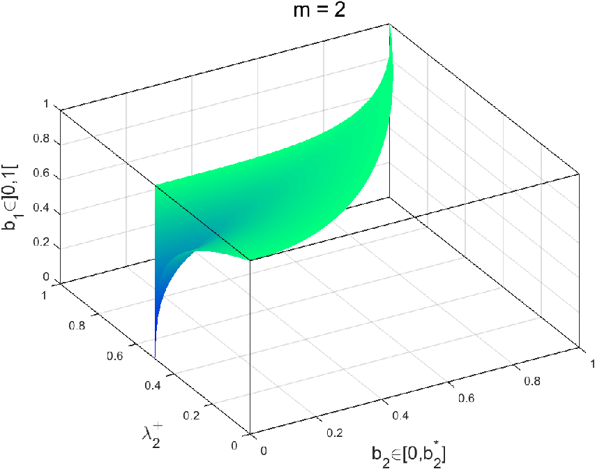
Refer to caption
Refer to caption
Refer to caption
Figure 8. λm±\lambda_{m}^{\pm} as a function of b2∈[0,bm⋆]b_{2}\in[0,b_{m}^{\star}], for m=2,3,4m=2,3,4, and for all b1∈]0,1[b_{1}\in]0,1[.

As in the simply-connected case, we use Ω=(1−λ)/2\Omega=(1-\lambda)/2 as our bifurcation parameter. In order to treat the saddle-node bifurcation points [26] that may appear during the bifurcation process, we use again the techniques described in [19].

Before illustrating the shape of the doubly-connected VV-states, let us mention that the situation is much more involved than in the simply-connected case, where there were roughly two situations for all mm: bb close to one, and bb not so close to one. Indeed, we have to play now with both the proximity of b1b_{1} to one, and that of b2b_{2} to bm⋆b_{m}^{\star}. Furthermore, we can start the bifurcation from the annulus of radii b1b_{1} and b2b_{2} at two different values of Ω\Omega, i.e., Ωm+\Omega_{m}^{+} and Ωm−\Omega_{m}^{-}. Finally, the case m=1m=1 needs to be studied individually. All in all, we have detected the following scenarios.

When m≥3m\geq 3, there are roughly three cases, when starting to bifurcate at Ωm+\Omega_{m}^{+}; and two cases, when starting to bifurcate at Ωm−\Omega_{m}^{-}. More precisely, if we start to bifurcate at Ωm+\Omega_{m}^{+}, we have to distinguish whether:

  • •

    b2b_{2} is very close to bm⋆b_{m}^{\star}. In that case, it seems possible to obtain VV-states for all Ω∈]Ωm−,Ωm+[\Omega\in]\Omega_{m}^{-},\Omega_{m}^{+}[, very much like in [22], irrespectively of the size of b1b_{1}. For example, in Figure 9, we have calculated the VV-states corresponding to m=4m=4, b1=0.8b_{1}=0.8, b2=0.53b_{2}=0.53. Observe that b4⋆=0.5407​…b_{4}^{\star}=0.5407\ldots, i.e., we have chosen b2b_{2} close enough to b4⋆b_{4}^{\star}. On the right-hand side, we have plotted the bifurcation diagram of the coefficients a1,1a_{1,1} and a2,1a_{2,1} in (92) against Ω\Omega, which shows that there is indeed a continuous bifurcation branch that joins Ωm−\Omega_{m}^{-} and Ωm+\Omega_{m}^{+}, where Ω4−=0.1335​…\Omega_{4}^{-}=0.1335\ldots, Ω4+=0.1671​…\Omega_{4}^{+}=0.1671\ldots. On the left-hand side, we have plotted VV-states for four different values of Ω∈]Ωm−,Ωm+[\Omega\in]\Omega_{m}^{-},\Omega_{m}^{+}[.

    Refer to caption
    Refer to caption
    Figure 9. Left: VV-states corresponding to m=4m=4, b1=0.8b_{1}=0.8, b2=0.53b_{2}=0.53, and several values of Ω\Omega. Right: bifurcation diagram. N=256N=256.
  • •

    b1b_{1} is close to one, and b2b_{2} is small enough, there are limiting VV-states, for which the distance between the outer boundary z1z_{1} and the unit circumference tends to zero; but the inner boundary z2z_{2} does not deviate greatly from the circumference of radius b2b_{2}. On the left-hand side of Figure 10, we have approximated the limiting VV-state corresponding to m=4m=4, b1=0.8b_{1}=0.8, b2=0.3b_{2}=0.3. The shape of z1z_{1} is not very far from the case m=4m=4, b=0.8b=0.8 of Figure 5.

    Refer to caption
    Refer to caption
    Figure 10. Approximation to the limiting VV-states corresponding to m=4m=4, b1=0.8b_{1}=0.8, b2=0.3b_{2}=0.3. Left: we have started to bifurcate at Ω4+=0.3256​…\Omega_{4}^{+}=0.3256\ldots, taking Ω<Ω4+\Omega<\Omega_{4}^{+}. Right: we have started to bifurcate at Ω4−=0.1250​…\Omega_{4}^{-}=0.1250\ldots, taking Ω>Ω4−\Omega>\Omega_{4}^{-}. N=1024N=1024.
  • •

    b1b_{1} and b2b_{2} do not fit in the previous two cases. In that case, there are also limiting VV-states, characterized by the appearance of corner-shaped singularities in z1z_{1} or z2z_{2}. In Figure 11, we have approximated the limiting VV-states corresponding to m=4m=4, b1=0.8b_{1}=0.8, b2=0.4b_{2}=0.4 (left); and to m=4m=4, b1=0.6b_{1}=0.6, b2=0.3b_{2}=0.3 (right). Observe that the influence of the rigid boundary seems less perceptible in the second example, which, accordingly, does not differ too much from those in [22].

    Refer to caption
    Refer to caption
    Figure 11. Left: Approximation to the limiting VV-state corresponding to m=4m=4, b1=0.8b_{1}=0.8, b2=0.4b_{2}=0.4, starting to bifurcate at Ω4+=0.2706\Omega_{4}^{+}=0.2706, taking Ω<Ω4+\Omega<\Omega_{4}^{+}. Right: Approximation to the limiting VV-state corresponding to m=4m=4, b1=0.6b_{1}=0.6, b2=0.3b_{2}=0.3, starting to bifurcate at Ω4+=0.2516\Omega_{4}^{+}=0.2516, taking Ω<Ω4+\Omega<\Omega_{4}^{+}. N=1024N=1024.

    Although the distance between z1z_{1} and the unit circumference is always strictly positive; the distance between z1z_{1} and z2z_{2} is sometimes very small, and we can not exclude in advance the existence of limiting VV-states where z1z_{1} and z2z_{2} actually touch each other. For instance, after playing with the values of b1b_{1} and b2b_{2}, we have found that the choice of b1=0.72b_{1}=0.72, b2=0.32b_{2}=0.32 enables us to find a VV-state, such that the distance between z1z_{1} and z2z_{2} is of about 7×10−37\times 10^{-3}. This VV-state is plotted in Figure 12, together with a zoom of one apparent intersection of the boundaries, that shows that there is really no intersection, and that the nodal resolution is adequate.

    Refer to caption
    Figure 12. Approximation to the limiting VV-state corresponding to m=4m=4, b1=0.72b_{1}=0.72, b2=0.32b_{2}=0.32, starting to bifurcate at Ω4+=0.2851\Omega_{4}^{+}=0.2851, taking Ω<Ω4+\Omega<\Omega_{4}^{+}. N=2048N=2048. The zoom shows that that the boundaries are very close from each other, but there is no intersection.

On the other hand, if we start to bifurcate at Ωm−\Omega_{m}^{-}, we have to distinguish whether:

  • •

    b2b_{2} is very close to bm⋆b_{m}^{\star}. This case has been explained above. In fact, it is irrelevant whether we start to bifurcate at Ωm−\Omega_{m}^{-} or at Ωm+\Omega_{m}^{+}.

  • •

    b2b_{2} is not close enough to bm⋆b_{m}^{\star}. In that case, there are limiting VV-states, characterized by the appearance of corner-shaped singularities in z2z_{2}, whereas the outer boundary z1z_{1} does not deviate greatly from the circumference of radius b1b_{1}. On the right-hand side of Figure 10, we have approximated the limiting VV-state corresponding to m=4m=4, b1=0.8b_{1}=0.8, b2=0.3b_{2}=0.3. We have not bothered to plot the VV-states corresponding to those in Figures 11 and 12, but starting to bifurcate at Ωm−\Omega_{m}^{-}, because they are virtually identical, up to a scaling of z2z_{2}. This case closely matches that in [22], and the inner boundary resembles the simply-connected VV-states in [11].

Summarizing, if we compare the doubly-connected VV-states just described, with those in [22], we conclude that the truly unique case here is when b1b_{1} is close to one, and b2b_{2} is small enough. In what regards the case m=2m=2, everything said above is applicable. For example, in Figure 13, we have taken b1=0.9b_{1}=0.9 and b1=0.2b_{1}=0.2, i.e., a value of b1b_{1} close to one and a value of b2b_{2} small enough. On the left-hand side, we show an approximation to the limiting VV-state appearing when starting to bifurcate at Ω2+\Omega_{2}^{+}; note the clear parallelism with the case m=2m=2, b=0.9b=0.9 of Figure 5, and with the left-hand side of Figure 10. On the right-hand side, we show an approximation to the limiting VV-state appearing when starting to bifurcate at Ω2−\Omega_{2}^{-}; as in the right-hand side of Figure 10, corner-shaped singularities seem to d evelop in z2z_{2}, whereas z1z_{1} has barely deviated from a circumference.

Refer to caption
Refer to caption
Figure 13. Left: Approximation to the limiting VV-states corresponding to m=2m=2, b1=0.9b_{1}=0.9, b2=0.2b_{2}=0.2, starting to bifurcate at Ω2+=0.3892​…\Omega_{2}^{+}=0.3892\ldots, taking Ω<Ω2+\Omega<\Omega_{2}^{+}. Right: we have started to bifurcate at Ω2−=0.2497​…\Omega_{2}^{-}=0.2497\ldots, taking Ω>Ω2−\Omega>\Omega_{2}^{-}. N=512N=512.

The case m=1m=1 deserves also some comment. In Figure 14, we have approximated the limiting VV-states corresponding to m=1m=1, taking again a value of b1b_{1} close to one and a value of b2b_{2} small enough, more precisely, b1=0.9b_{1}=0.9, b2=0.3b_{2}=0.3. On the left-hand side, we have started to bifurcate at Ω1+\Omega_{1}^{+}; and on the right-hand side, we have started to bifurcate at Ω1−\Omega_{1}^{-}. It is remarkable that, in both cases, the distance of z1z_{1} to the unit circumference is smaller than 10−210^{-2}. Moreover, even if the VV-state on the left-hand side is roughly in agreement with Figure 5, and with the left-hand sides of Figures 10 and 13; the VV-state on the right-hand side exhibits a completely different, unexpected behavior.

Refer to caption
Refer to caption
Figure 14. Approximation to the limiting VV-states corresponding to m=1m=1, b1=0.9b_{1}=0.9, b2=0.3b_{2}=0.3. Left: we have started to bifurcate at Ω1+=4/9\Omega_{1}^{+}=4/9, taking Ω<Ω1+\Omega<\Omega_{1}^{+}. Right: we have started to bifurcate at Ω1−=0.36\Omega_{1}^{-}=0.36, taking Ω>Ω1−\Omega>\Omega_{1}^{-}. N=256N=256.

Acknowledgements. Francisco de la Hoz was supported by the Basque Government, through the project IT641-13, and by the Spanish Ministry of Economy and Competitiveness, through the project MTM2014-53145-P. Taoufik Hmidi was partially supported by the ANR project Dyficolti ANR-13-BS01-0003- 01. Joan Mateu was partially supported by the grants of Generalitat de Catalunya 2014SGR7, Ministerio de Economía y Competitividad MTM 2013-4469, ECPP7- Marie Curie project MAnET.

References

  • [1] A. L. Bertozzi and P. Constantin. Global regularity for vortex patches. Comm. Math. Phys., 152 (1993), no. 1, 9–28.
  • [2] A. L. Bertozzi and A. J. Majda. Vorticity and Incompressible Flow. Cambridge texts in applied Mathematics, Cambridge University Press, Cambridge, (2002).
  • [3] J. Burbea. Motions of vortex patches. Lett. Math. Phys. 6 (1982), no. 1, 1–16.
  • [4] J. Burbea, M. Landau. The Kelvin waves in vortex dynamics and their stability. Journal of Computational Physics, 45(1982) 127–156.
  • [5] J. Burbea. Vortex motions and conformal mappings. Nonlinear evolution equations and dynamical systems (Proc. Meeting, Univ. Lecce, Lecce, 1979), pp. 276Ð298, Lecture Notes in Phys., 120, Springer, Berlin-New York, 1980.
  • [6] A. Castro, D. Córdoba, J. Gómez-Serrano. Existence and regularity of rotating global solutions for the generalized surface quasi-geostrophic equations. arXiv:1409.7040.
  • [7] A. Castro, D. Córdoba, J. Gómez-Serrano. Uniformly rotating analytic global patch solutions for active scalars, arXiv:1508.01655
  • [8] C. Cerretelli, C. H. K. Williamson. A new family of uniform vortices related to vortex configurations before Fluid merger. J. Fluid Mech. 493 (2003) 219–229.
  • [9] J.-Y. Chemin. Perfect incompressible Fluids. Oxford University Press 1998.
  • [10] M. G. Crandall, P. H. Rabinowitz. Bifurcation from simple eigenvalues. J. of Func. Analysis 8 (1971), 321–340.
  • [11] G. S. Deem, N. J. Zabusky. Vortex waves: Stationary "VV-states", Interactions, Recurrence, and Breaking. Phys. Rev. Lett. 40 (1978), no. 13, 859–862.
  • [12] N. Depauw. Poche de tourbillon pour Euler 2D dans un ouvert à bord. J. Math. Pures Appl. (9) 78 (1999), no. 3, 313–351.
  • [13] D. G. Dritschel. The nonlinear evolution of rotating configurations of uniform vorticity, J. Fluid Mech. 172 (1986), 157–182.
  • [14] R. Farwig, T. Hishida. Asymptotic profile of steady Stokes flow around a rotating obstacle. Manuscripta Math. 136 (2011), no. 3-4, 315–338.
  • [15] G. R. Flierl, L. M. Polvani. Generalized Kirchhoff vortices. Phys. Fluids 29 (1986), 2376–2379.
  • [16] L. E. Fraenkel. An introduction to maximum principles and symmetry in elliptic problems. Cambridge Tracts in Mathematics, 128. Cambridge University Press, Cambridge, 2000.
  • [17] Y. Guo, C. Hallstrom, D. Spirn. Dynamics near an unstable Kirchhoff ellipse. Comm. Math. Phys., 245(2):297Ð354, 2004.
  • [18] Z. Hassainia, T. Hmidi. On the VV-states for the generalized quasi-geostrophic equations. Comm. Math. Phys. 337 (2015), no. 1, 321–377.
  • [19] Z. Hassainia, T. Hmidi, F. de la Hoz. Doubly-connected VV-states for the generalized surface quasi-geostrophic equations. Preprint arXiv:1412.4587.
  • [20] T. Hmidi, J. Mateu, J. Verdera. Boundary Regularity of Rotating Vortex Patches. Arch. Ration. Mech. Anal. 209 (2013), no. 1, 171–208.
  • [21] T. Hmidi, J. Mateu, J. Verdera. On rotating doubly-connected vortices. J. Differential Equations 258 (2015), no. 4, 1395–1429.
  • [22] T. Hmidi, F. de la Hoz, J. Mateu, J. Verdera. Doubly-connected VV-states for the planar Euler equations. arXiv:1409.7096.
  • [23] T. Hmidi. On the trivial solutions for the rotating patch model, to appear in J. Evol. Equ., arXiv:1409.8469.
  • [24] T. Hmidi, J. Mateu. Bifurcation of rotating patches from Kirchhoff vortices. arXiv:1508.04589
  • [25] J. R. Kamm. Shape and stability of two-dimensional uniform vorticity regions. PhD thesis, California Institute of Technology, 1987.
  • [26] H. Kielhöfer. Bifurcation Theory: An introduction with applications to partial differential equations, Springer ( 2011)
  • [27] G. Kirchhoff. Vorlesungen uber mathematische Physik (Leipzig, 1874).
  • [28] H. Lamb. Hydrodynamics, Dover Publications, New York, (1945).
  • [29] A. E. H. Love. On the Stability of certain Vortex Motions. Proc. London Math. Soc., 25(1)18–42, 1893.
  • [30] P. Luzzatto-Fegiz, C. H. K. Williamson. Stability of elliptical vortices from ÒImperfect-Velocity-ImpulseÓ diagrams. Theor. Comput. Fluid Dyn., 24 (2010), 1-4, 181–188.
  • [31] T. B. Mitchell and L. F. Rossi.The evolution of Kirchhoff elliptic vortices. Physics of Fluids, 20(5), 2008.
  • [32] E. A. II Overman. Steady-state solutions of the Euler equations in two dimensions. II. Local analysis of limiting VV-states. SIAM J. Appl. Math. 46 (1986), no. 5, 765–800.
  • [33] H. Plotka, D. G. Dritschel. Quasi-geostrophic shallow-water vortex-patch equilibria and their stability. Geophys. Astrophys. Fluid Dyn. 106 (2012), no. 6, 574–595
  • [34] Ch. Pommerenke. Boundary behaviour of conformal maps. Springer-Verlag, Berlin, (1992).
  • [35] P. G. Saffman. Vortex dynamics. Cambridge Monographs on Mechanics and Applied Mathematics. Cambridge University Press, New York, 1992.
  • [36] Y. Tang. Nonlinear stability of vortex patches. Trans. Amer. Math. Soc., 304(2)617–638, 1987.
  • [37] Y. H. Wan. The stability of rotating vortex patches. Comm. Math. Phys., 107(1) 1–20, 1986.
  • [38] S. E. Warschawski. On the higher derivatives at the boundary in conformal mapping, Trans. Amer. Math. Soc. 38 (1935), no. 2, 310–340.
  • [39] H. M. Wu, E.A. II Overman, N. J. Zabusky. Steady-state solutions of the Euler equations in two dimensions : rotating and translating VV-states with limiting cases I. Algorithms ans results, J. Comput. Phys. 53 (1984), 42–71.
  • [40] Y. Yudovich. Nonstationary flow of an ideal incompressible liquid. Zh. Vych. Mat., 3, (1963), 1032–1066.