On the number of unary-binary tree-like structures with restrictions on the unary height

Olivier Bodini ^†^†thanks: Institut Galilée, Univ. Paris 13, Villetaneuse (France). Supported by ANR Metaconc project (France) 2015-18 Danièle Gardy ^†^†thanks: DAVID Laboratory, University of Versailles Saint Quentin en Yvelines. Part of the work of this author was done during a long-term visit at the Institute of Discrete Mathematics and Geometry of the TU Wien. Partially supported by the P.H.C. Amadeus project Boolean expressions: compactification, satisfiability and distribution of functions (2013-14) and by the ANR project BOOLE (2009-13). Bernhard Gittenberger ^†^†thanks: Institute for Discrete Mathematics and Geometry, Technische Universität Wien, Wiedner Hauptstrasse 8-10/104, A-1040 Wien, Austria. Supported by FWF grant SFB F50-03 and ÖAD, grant F01/2015 Zbigniew Gołębiewski ^†^†thanks: Institute for Discrete Mathematics and Geometry, Technische Universität Wien, Wiedner Hauptstrasse 8-10/104, A-1040 Wien, Austria. Supported by FWF grant SFB F50-03

Abstract

We consider various classes of Motzkin trees as well as lambda-terms for which we derive asymptotic enumeration results. These classes are defined through various restrictions concerning the unary nodes or abstractions, respectively: We either bound their number or the allowed levels of nesting. The enumeration is done by means of a generating function approach and singularity analysis. The generating functions are composed of nested square roots and exhibit unexpected phenomena in some of the cases. Furthermore, we present some observations obtained from generating such terms randomly and explain why usually powerful tools for random generation, such as Boltzmann samplers, face serious difficulties in generating lambda-terms.

1 Introduction

This paper is mainly devoted to the asymptotic enumeration of lambda-terms belonging to a certain subclass of the class of all lambda-terms. Roughly speaking, a lambda-term is a formal expression built of variables and a quantifier $\lambda$ which in general occurs more than once and acts on one of the free variables of the subsequent sub-term. Lambda calculus is a set of rules for manipulating lambda-terms and was invented by Church and Kleene in the 30ies (see [35, 36, 16]) in order to investigate decision problems. It plays an important rôle in computability theory, for automatic theorem proving or as a basis for some programming languages, e.g. LISP. Due to its flexibility it can be used for a formal description of programming in general and is therefore an essential tool for analyzing programming languages (cf. [37, 38]) and is now widely used in artificial intelligence. Furthermore, in typed lambda calculus types can be interpreted as logical propositions and lambda-terms of a given type as proofs of the corresponding proposition. This is known as the Curry-Howard isomorphism (see [45]) and constitutes in view of the above-mentioned link to programming a direct relationship between computer programs and mathematical proofs.

Recently, there has been rising interest in random structures related to logic in general (see [48] [27], [28], and [19]) and in the properties of random lambda-terms in particular (see [18], [30] or [39]).

Although lambda-terms are related to Motzkin trees, the counting sequences of these two objects have widely different behaviours. In this paper, a tree-like behaviour is meant to be that the counting sequence asymptotically behaves as is typical for trees with average height asymptotically proportional to the root of the tree size. See [20] for numerous results on such trees as well as many other classes of trees. For analyzing the structure of random lambda-terms it is important to know the number of lambda-terms of a given size. It turns out that this is a very hard problem. The reason is that there are many degrees of freedom for assigning variables to a given abstraction. This leads to a large number of lambda-terms of fixed size. If we translate the counting problem into generating functions, then the resulting generating function has radius of convergence equal to zero. Thus none of the classical methods of analytic combinatorics (see [25]) is applicable. Therefore, in this paper we study simpler structures, obtained by bounding either the total number of abstractions or by introducing bounds on the levels of nesting (either globally or locally, to be formally defined in the next section) of lambda-terms. Note that the number of nesting levels of abstraction or even the number of abstractions in lambda-terms which occur in computer programming is in general assumed low compared to their size. E.g., for implementing lambda-calculus we need to bound the height of the underlying stack, which is determined by the maximal allowed number of nested abstractions. Even more, Yang et al. [47], who developed the very successful software Csmith for finding bugs in real programs like the gcc compiler, write on [47, p. 3]: “Csmith begins by randomly creating a collection of struct type declarations. For each, it randomly decides on a number of members and the type of each member. The type of a member may be a (possibly qualified) integral type, a bit-field, or a previously generated struct type.” A declaration in a C program corresponds to an abstraction in a lambda-term, and the engineers chose the number of abstractions before randomly generating the rest of the program. That means that they expect the number of abstractions to be independent of the size of the lambda-term which corresponds to their program. Thus, requiring bounds like those mentioned above seems not to be a severe restriction from a practical point of view.

Preliminary results on the enumeration of lambda-terms with bounded unary height appeared in [5].

The plan of the paper is as follows: We present all the formal definitions of the objects of our interest in Section 2 and then, in Section 3, some results on restricted classes of Motzkin trees for comparison purposes. The enumeration of lambda-terms with a fixed or bounded number of unary nodes is done in Section 4. Sections 5 and 6 contain the main results of our paper. They are devoted to the enumeration of lambda-terms where all bindings have bounded unary length and lambda-terms with bounded unary height, respectively. In order to achieve our results, we first derive generating functions for the associated counting problems, which are expressed as a finite nesting of radicals. Then we study the radii of convergence and the type of their singularities. This will eventually allows us to determine their number asymptotically, as their size tends to infinity. A comparison of the two classes of lambda-terms is discussed in Section 7. Finally, we investigate how our theoretical results fit with simulations and discover some challenging facts on the average behaviour of a random lambda-term in Section 8.

2 A combinatorial description for lambda-terms

2.1 Representation as directed acyclic graphs

A lambda-term is a formal expression which is described by the context-free grammar

T::=a\;\mid\;(T*T)\;\mid\;\lambda a.T

where $a$ is a variable. The operation $(T*T)$ is called application. Using the quantifier $\lambda$ is called abstraction. Furthermore, each abstraction binds a variable and each variable can be bound by at most one abstraction. A variable which is not bound by an abstraction is called free. A lambda-term without free variables is called closed, otherwise open.

In this paper we deal with the enumeration of $\alpha$ -equivalence classes of closed lambda-terms: Two terms are $\alpha$ -equivalent if one term can be transformed into the other one by a sequence of $\alpha$ -conversions. An $\alpha$ -conversion is the renaming of a bound variable in the whole term (cf. [3]). Since the lambda-terms we consider are closed, this means that the actual variable names are unimportant; only the structure of the bindings is relevant. E.g., we consider the terms $\lambda x.x$ and $\lambda y.y$ to be identical.

Furthermore, note that neither application nor iterated abstraction is commutative, i.e., in particular, the terms $\lambda x.\lambda y.T$ and $\lambda y.\lambda x.T$ are different (if and only if at least one variable $x$ or $y$ appears in $T$ ).

A lambda-term can be represented as an enriched tree, i.e., a graph built from a rooted tree by adding certain directed edges (pointers). First we construct a Motzkin tree, i.e., a plane rooted tree where each node has out-degree 0, 1, or 2, if the edges were directed away from the root. We denote by the terms leaves, unary nodes, and binary nodes, the nodes with out-degree 0, 1, and 2, respectively. In this tree each application corresponds to a binary node, each abstraction to a unary node, and each variable to a leaf. The fact that an abstraction $\lambda$ binds a variable $v$ is represented by adding a directed edge from the unary node corresponding to the particular abstraction $\lambda$ to the leaf labelled by $v$ . Therefore, each unary node $x$ of the Motzkin tree is carrying (zero, one or more) pointers to leaves taken from the subtree rooted at $x$ ; all leaves receiving a pointer from $x$ correspond to the same variable, and each leaf can receive at most one pointer. The Motzkin tree obtained from a lambda-term $t$ by removing all pointers (variable bindings) is called the underlying tree of $t$ .

For instance, the terms $(\lambda x.(x*x)*\lambda y.y)$ and $\lambda y.(\lambda x.x*\lambda x.y)$ correspond to the enriched trees $T_{0}$ and $T_{1}$ in Fig. 1, respectively. In particular, these terms are closed lambda-terms, because every variable is bound by an abstraction, i.e., every leaf receives exactly one pointer.

Refer to caption — Figure 1: Two examples of lambda-terms (or $\alpha$ -equivalence classes if the labels of the leaves are removed): Each unary node corresponds to an abstraction $\lambda x$ binding all leaves below it which are labelled by $x$ . Binary nodes correspond to applications merging their two subtrees $t_{1}$ and $t_{2}$ into the more complex structure $t_{1}*t_{2}$ .

As mentioned in the introduction, our interest in the present paper is in lambda-terms with restrictions on the number of abstractions and on the number of nesting levels of abstraction, either locally or globally. The following definitions will allow us to state our restrictions more precisely.

Definition 1.

Consider a lambda-term and its associated enriched tree $T$ . The unary length of the binding of a leaf $e$ by some abstraction $v$ in $T$ (directed edge from $v$ to $e$ ), denoted by $l_{u}(e)$ , is defined as a number of unary nodes on the path connecting $v$ and $e$ in the underlying Motzkin tree.

Definition 2.

Consider a lambda-term and its associated enriched tree $T$ . The unary height of a vertex $v$ of $T$ , denoted by $h_{u}(v)$ , is defined as number of unary nodes on the path from the root to $v$ in the underlying Motzkin tree. The unary height of $T$ , $h_{u}(T)$ , is defined by $\max\limits_{\mbox{\scriptsize$v$ \rm vertex of $T$}}h_{u}(v)$ . We use the same notions for Motzkin trees as well.

In this paper we will enumerate lambda-terms with a fixed number of unary nodes, with bounded unary length of the bindings, or with bounded unary height. Of course, other simplifications are possible, such as bounding the number of pointers for each unary node. Such terms are related to linear (terms where each abstraction binds at most one variable, also called BCI terms) and affine (terms where each abstraction binds at most one variables, also called BCK terms) logics as introduced in [3, 33, 32, 34], and their enumeration was treated in [7] and generalizations can be found in [6] and [9]. For their relations to lambda-calculus see for instance [31].

2.2 Generating functions associated with lambda-terms

For each class of lambda-terms we will enumerate the terms of a given size. The size of a lambda-term is the number of nodes in the corresponding enriched tree. It is defined recursively by

	$\displaystyle\|x\|$	$\displaystyle=1,$
	$\displaystyle\|\lambda x.T\|$	$\displaystyle=1+\|T\|,$
	$\displaystyle\|(S*T)\|$	$\displaystyle=1+\|S\|+\|T\|.$

In order to count $\alpha$ -equivalence classes of lambda-terms of a given size we set up a formal equation which is then translated into a functional equation for generating functions using the well-known symbolic method (cf. [25]).

Let us introduce the following atomic classes: the class of application nodes $\mathcal{A}$ , the class of abstraction nodes $\mathcal{U}$ , the class of free leaves $\mathcal{F}$ , and the class of bound leaves $\mathcal{D}$ . Then the class $\mathcal{L}$ of equivalence classes of lambda-terms can be described by the specification

\mathcal{L}=\mathcal{F}+\left(\mathcal{A}\times\mathcal{L}^{2}\right)+\left(\mathcal{U}\times\rm{subs}(\mathcal{F}\to\mathcal{F}+\mathcal{D},\mathcal{L})\right).

(1)

where the substitution operator $\rm{subs}(\mathcal{F}\to\mathcal{F}+\mathcal{D},\mathcal{L})$ corresponds to replacing some free leaves in $\mathcal{L}$ by bound leaves.

Remark 1.

Note that the lambda-terms specified by $\mathcal{L}$ are not necessarily closed. Since $\alpha$ -conversion concerns only the bound variables, the equivalence here is w.r.t. $\alpha$ -conversion and substitution of a free variable by another free variable which is not already present in the term.

The specification (1) gives rise to a functional equation for the bivariate generating function

L(z,f)=\sum_{t\;\;\mbox{\scriptsize lambda-term}}z^{|t|}f^{\#\mbox{\scriptsize free leaves in }t}

which reads as follows:

L(z,f)=fz+zL(z,f)^{2}+zL(z,f+1).

(2)

In particular, the formal generating function for lambda-terms without free variables is

	$\displaystyle L(z,0)$	$\displaystyle=[f^{0}]L(z,f)$
		$\displaystyle=z^{2}+2z^{3}+4z^{4}+13z^{5}+42z^{6}+139z^{7}+506z^{8}+1915z^{9}+7558z^{10}+\cdots$

Note that these functional equations have to be considered in the framework of formal power series since the fast growth of the coefficients of the generating function implies that the radius of convergence of $L(z,0)$ is zero (see Corollary 3 below).

Furthermore note, that the problem of counting closed or open lambda-terms is essentially the same. Indeed, the formal generating function for open lambda-terms can be derived from Eq. (2) the formula $L(z,1)-L(z,0)=\frac{(1-z)L(z,0)-zL(z,0)^{2}}{z}.$ Consequently, the problems of enumerating lambda-terms with or without free variables are of the same difficulty and the solution for one of them yields the solution for the other one.

Before we start with the analysis of the generating functions associated with the considered combinatorial structures let us introduce a few further notions.

Definition 3.

We say that a function $f:\mathbb{C}\to\mathbb{C}$ has a singularity of type $\alpha$ at $z=\rho$ if there is a constant $c$ such that

f(z)\sim c\left(1-\frac{z}{\rho}\right)^{\alpha},

as $z\to\rho$ inside the domain of analyticity of $f$ .

Definition 4.

If $f:\mathbb{C}\to\mathbb{C}$ is a function which is analytic at 0. Then let $S$ denote the set of all singularities of $f$ which lie on the circle of convergence of the Taylor series of $f$ (expanded at $z=0$ ). Those singularities in $S$ which are of smallest type are called the dominant singularities of $f$ .

Remark 2.

It is well-known since Darboux [17] that the singularities on the circle of convergence determine the asymptotic behaviour of the coefficients of a series. The transfer theorems of Flajolet and Odlyzko [24] make this much more precise and show that indeed only the dominant singularity in the sense of the definition above and its type yield the (main term of the) asymptotic behaviour.

3 Restricted Motzkin trees

Before considering restricted lambda-terms, we present results on classes of restricted Motzkin trees. We shall consider classes of Motzkin trees with restrictions analogous to those for lambda-terms, namely a fixed or bounded number of unary nodes, and a fixed or bounded unary height, where the unary height of a leaf is the number of unary nodes on the path from the root to that leaf, and the unary height of a tree is the maximal unary height of a leaf.

The size of a Motzkin tree is defined as the total number of nodes. The generating function associated with Motzkin trees satisfies the functional equation $M(z)=z+zM(z)+zM^{2}(z).$ Solving this equation shows that the only power series solution is

M(z)=\frac{1}{2z}\left(1-z-\sqrt{1-2z-3z^{2}}\right).

The roots of the radicand are $-1$ and $1/3$ , the latter being the dominant singularity of $M(z)$ and of type $\frac{1}{2}$ . Applying a transfer theorem from [24] yields that the number of Motzkin trees of size $n$ is asymptotically $[z^{n}]M(z)\sim\frac{3^{n+\frac{1}{2}}}{2n\sqrt{\pi n}}$ .

3.1 Restrictions on the total number of unary nodes

Let $\mathcal{M}_{q}$ be the class of Motzkin trees with exactly $q$ unary nodes. We point out that a Motzkin tree with exactly $q$ unary nodes has a total size $n$ equal to $q+1+2m$ , where $m$ is the number of binary nodes and $m+1$ the number of leaves.

Proposition 1.

The number of Motzkin trees of size $n$ with exactly $q$ unary nodes is 0 if $n\equiv q\mod 2$ ; otherwise it is asymptotically equivalent to $\sqrt{\frac{2}{\pi}}\,\frac{1}{2^{q}\,q!}\,2^{n}n^{q-\frac{3}{2}}$ , as $n\to\infty$ and for fixed $q$ .

Proof.

The assertion is an immediate consequence of Tutte’s theorem [46] which implies directly that the number of Motzkin trees of size $n$ with exactly $q$ unary nodes is $\frac{(n-1)!}{q!((n-q-1)/2)!}$ . ∎

For self-containedness and as it is in the flavour of this paper, we offer a proof of Proposition 1 based on analytic combinatorics.

Obviously $\mathcal{M}_{0}=\mathcal{C}$ is the class of binary Catalan trees and its generating function is $M_{0}(z)=C(z)=\frac{1-\sqrt{1-4z^{2}}}{2z}$ . For $q\geq 1$ we have $\mathcal{M}_{q}=\mathcal{U}\times\mathcal{M}_{q-1}+\sum_{\ell=0}^{q}\mathcal{A}\times\mathcal{M}_{\ell}\times\mathcal{M}_{q-\ell}.$ This equation translates into a functional equation for the generating functions and we get (after solving w.r.t. $M_{q}(z)$ )

M_{q}(z)=\frac{zM_{q-1}(z)+z\,\sum_{1\leq\ell\leq q-1}M_{\ell}(z)M_{q-\ell}(z)}{1-2zM_{0}(z)}.

(3)

Lemma 1.

There exists a sequence of polynomials sequence $(P_{q}(z))_{q\geq 2}$ such that

M_{q}(z)=\frac{z^{q+1}P_{q}(z^{2})}{(1-4z^{2})^{q-\frac{1}{2}}},\text{ for }q\geq 2.

(4)

The polynomials $P_{q}(z)$ are given by the recurrence relation

P_{2}(z)=1;\qquad P_{q}(z)=P_{q-1}(z)+z\sum_{l=2}^{q-2}P_{l}(z)P_{q-l}(z)\qquad(q\geq 3).

(5)

Proof.

For convenience set $\Delta=1-2zM_{0}(z)=\sqrt{1-4z^{2}}$ . From (3) one easily derives that $M_{2}=z^{3}/\Delta^{3}$ which fits with the assertion (4). We assume that the assumption $M_{\ell}=\frac{z^{\ell+1}P_{\ell}(z^{2})}{\Delta^{2\ell-1}}$ holds for $\ell=2,\dots,q-1$ ; Eq. (3) then gives

	$\displaystyle M_{q}(z)$	$\displaystyle=\frac{z}{\Delta}\;\left((1+2M_{1}(z))M_{q-1}(z)+\sum_{\ell=2}^{q-2}M_{\ell}(z)M_{q-\ell}(z)\right)$
		$\displaystyle=\frac{z}{\Delta}\;\left(\frac{M_{q-1}(z)}{\Delta}+\sum_{\ell=2}^{q-2}M_{\ell}(z)M_{q-\ell}(z)\right)$
		$\displaystyle=\frac{z}{\Delta}\left(\frac{z^{q}P_{q-1}(z^{2})}{\Delta^{2q-2}}+\sum_{\ell=2}^{q-2}\frac{z^{\ell+1}P_{\ell}(z^{2})}{\Delta^{2\ell-1}}\cdot\frac{z^{q-\ell+1}P_{q-\ell}(z^{2})}{\Delta^{2(q-\ell)-1}}\right)$
		$\displaystyle=\frac{z^{q+1}}{\Delta^{2q-1}}\;\left(P_{q-1}(z^{2})+z^{2}\;\sum_{\ell=2}^{q-2}P_{\ell}(z^{2})P_{q-\ell}(z^{2})\right).$

From the last formula we read off the recurrence relation (5) and get the assertion after all. ∎

The asymptotic behaviour of the coefficients of $M_{q}(z)$ is now readily obtained (recall that $n=q+1+2m$ , with $m$ being the number of binary nodes):

[z^{n}]M_{q}(z)=[z^{2m}]\frac{P_{q}(z^{2})}{(1-4z^{2})^{q-\frac{1}{2}}}=[z^{m}]\frac{P_{q}(z)}{(1-4z)^{q-\frac{1}{2}}}\sim[z^{m}]\frac{4^{m}P_{q}(1/4)}{(1-z)^{q-\frac{1}{2}}}.

As $[z^{m}](1-z)^{-q+\frac{1}{2}}\sim\frac{m^{q-\frac{3}{2}}}{\Gamma(q-\frac{1}{2})}$ , we get

[z^{n}]M_{q}(z)\sim 2^{n-q-1}P_{q}(1/4)\frac{(n-q-1)^{q-\frac{3}{2}}}{2^{q-\frac{3}{2}}\Gamma(q-\frac{1}{2})}\sim\frac{P_{q}(1/4)\sqrt{2}}{4^{q}\Gamma(q-\frac{1}{2})}\,2^{n}n^{q-\frac{3}{2}}.

Set $a_{q}=P_{q}(1/4)$ ; then $a_{2}=a_{3}=1$ and $a_{q}=a_{q-1}+\frac{1}{4}\sum_{2\leq\ell\leq q-2}a_{\ell}a_{q-\ell}$ for $q\geq 4$ . This implies $a_{q}=2^{2-q}C_{q-1}$ where $C_{q}$ denotes the $q$ th Catalan number. Plugging this into the asymptotic expression for $[z^{n}]M_{q}(z)$ gives immediately Proposition 1.

Next we consider the number of Motzkin trees with at most $q$ unary nodes. Then we have $M_{\leq q}(z)=\sum_{0\leq r\leq q}M_{r}(z)$ and $[z^{n}]M_{\leq q}(z)=\sum_{0\leq r\leq q}[z^{n}]M_{r}(z)$ . Hence the last term of the sum gives the asymptotic main term which is $[z^{n}]M_{q}$ if $n\not\equiv q\mod 2$ , and $[z^{n}]M_{q-1}$ otherwise.

3.2 Restrictions on the unary height

Define $\mathcal{B}_{k}$ as the set of Motzkin trees such that all leaves are at the same unary height $k$ and $\mathcal{B}_{\leq k}$ as the set of Motzkin trees where leaves have unary height at most equal to $k$ .

3.2.1 All leaves at the same unary height

Again, we start with setting up the specification and translating them into functional equations for the generating functions.

Lemma 2.

The class $\mathcal{B}_{0}$ is equal to that of binary Catalan trees. Thus $B_{0}(z)=C(z)=(1-\sqrt{1-4z^{2}})/(2z)$ . For $k\geq 1$ we have the recursive specification $\mathcal{B}_{k}=\mathcal{U}\times\mathcal{B}_{k-1}+\mathcal{A}\times\mathcal{B}_{k}\times\mathcal{B}_{k}.$ Thus, the generating function associated with $\mathcal{B}_{k}$ satisfies

	$\displaystyle B_{k}(z)$	$\displaystyle=\frac{1}{2z}\left(1-\sqrt{1-4z^{2}B_{k-1}}\right)$
		$\displaystyle=\frac{1}{2z}\left(1-\sqrt{1-2z+2z\sqrt{1-2z+\dots+2z\sqrt{1-4z^{2}}}}\right),$

where the second expression has $k+1$ nested square roots.

Now we turn to the asymptotic behaviour of such bounded unary height trees. For $k=1$ , the dominant singularity of $B_{1}(z)$ is at $z=1/2$ and of type $\frac{1}{4}$ . The other singularity is at $z=-1/2$ , but of type $\frac{1}{2}$ and gives therefore an asymptotically negligible contribution. We obtain

[z^{n}]B_{1}(z)\sim\frac{1}{4}\cdot\frac{2^{\frac{1}{4}}2^{n}n^{-\frac{5}{4}}}{\Gamma\left(\frac{3}{4}\right)}.

Likewise, for $k\geq 2$ , the singularities of $B_{k}(z)$ are $\pm 1/2$ , which can easily be seen by induction. The singularity at $z=-1/2$ originates from the innermost radical only and is therefore of type $1/2$ . At $z=1/2$ all radicals vanish at once and hence the singularity is of type $1/2^{k+1}$ . Consequently, as $z\to 1/2$ , we have

B_{k}(z)=1-2^{2^{-k-1}}(1-2z)^{2^{-k-1}}(1+O(\sqrt{1-2z}\,)).

Determining the asymptotic behaviour is now straightforward.

Proposition 2.

The number of Motzkin trees in which all leaves have exactly unary height $k$ is

[z^{n}]B_{k}(z)\sim 2^{n+\alpha}\,\frac{n^{-1-\alpha}}{\Gamma(-\alpha)}\qquad with\qquad\alpha=\frac{1}{2^{k+1}}.

Remark 3.

This is another of the rather rare examples where the generating function of a recursively specified combinatorial structure does not have a dominant singularity of type 1/2 (or multiple of 1/2). A general discussion of possible singularity types of generating functions given by systems of functional equations was recently given by Banderier and Drmota [2].

3.2.2 Motzkin trees of bounded unary height

The case $k=0$ again corresponds to binary Catalan trees and for larger $k$ a similar recursive specification as in the previous subsection holds.

Lemma 3.

The class $\mathcal{B}_{\leq k}$ is equal to that of binary Catalan trees. For $k\geq 1$ we have the recursive specification $\mathcal{B}_{\leq k}=\mathcal{Z}+\mathcal{U}\times\mathcal{B}_{\leq k-1}+\mathcal{A}\times\mathcal{B}_{\leq k}\times\mathcal{B}_{\leq k}$ . Thus the generating function associated with $\mathcal{B}_{\leq k}$ satisfies

	$\displaystyle B_{\leq k}(z)$	$\displaystyle=\frac{1}{2z}\left(1-\sqrt{1-4z^{2}-4z^{2}B_{\leq k-1}}\right)$
		$\displaystyle=\frac{1}{2z}\left(1-\sqrt{1-2z-4z^{2}+2z\sqrt{1-2z-4z^{2}+\dots+2z\sqrt{1-4z^{2}}}}\right).$

where the second expression has $k+1$ nested square roots.

Again, the first function $B_{\leq 0}(z)$ has the two singularities $\pm 1/2$ , but the next ones have different singularities. Indeed, the innermost square root $\sqrt{1-4z^{2}}$ has a zero at $z=\pm 1/2$ , but the next radical, $\sqrt{1-2z-4z^{2}+2z\sqrt{1-4z^{2}}}$ , has a zero at $\tilde{\rho}_{1}=0.4064073933<1/2$ . The following few values are $\tilde{\rho}_{2}=0.3759923651$ , $\tilde{\rho}_{3}=0.3617581845$ , $\tilde{\rho}_{4}=0.3538076738$ .

Lemma 4.

Let $\tilde{R}_{0}(z)=1-4z^{2}$ and $\tilde{R}_{k}(z)=1-2z-4z^{2}+2z\sqrt{\tilde{R}_{k-1}(z)}$ . Then the values $\tilde{\rho}_{k}$ , defined as the smallest real positive root of $\tilde{R}_{k}(z)=0$ , form a decreasing sequence.

Proof.

An easy inductive argument shows that the functions $\tilde{R}_{k}(z)$ are decreasing functions on the positive real line (of course, only up to their first singularity) and smaller than 1 there: Note that for positive $z$ we get $\sqrt{\tilde{R}_{k-1}(z)}\leq 1\leq 1+4z$ .

Notice that the class of Motzkin trees of bounded unary height is a subclass of the class of unrestricted Motzkin trees. The generating function of the latter one has dominant singularity equals to $\frac{1}{3}$ . Hence, for any fixed $k$ , we must have $\tilde{\rho}_{k}\geq\frac{1}{3}$ .

Now, suppose that $\tilde{\rho}_{k-1}\leq\tilde{\rho}_{k}$ . Then, since $\tilde{R}_{k}(z)$ is decreasing for positive real $z$ and $\tilde{R}_{k-1}(\tilde{\rho}_{k-1})=0$ , we have $\tilde{R}_{k}(\tilde{\rho}_{k-1})=1-2\tilde{\rho}_{k-1}-4\tilde{\rho}_{k-1}^{2}\geq 0$ . But $1-2z-4z^{2}\geq 0$ if and only if $z\in\left[\frac{-\sqrt{5}-1}{4},\frac{\sqrt{5}-1}{4}\right]$ and $\frac{\sqrt{5}-1}{4}<1/3$ which contradicts the fact that $\tilde{\rho}_{k}\geq\frac{1}{3}$ for all $k$ . ∎

Remark 4.

Since the sequence $(\tilde{\rho}_{k})_{k\geq 0}$ is decreasing and bounded from below by $\frac{1}{3}$ , one can try to prove that $\tilde{\rho}_{k}\to\frac{1}{3}$ as $k\to\infty$ . Though numerical evidence supports this, it seems not obvious at all. Since it is not the key point of our paper we decided to skip it.

As $B_{\leq k}(z)=\left(1-\sqrt{\tilde{R}_{k}(z)}\right)/(2z)$ and each radical has a different dominant singularity, the dominant singularity of $B_{\leq k}$ is at $z=\tilde{\rho}_{k}$ and of type $1/2$ . Here the dominant singularity always comes from the outermost radical. Thus, we obtain the following result:

Proposition 3.

The number of Motzkin trees with unary height at most equal to $k$ is

[z^{n}]B_{\leq k}(z)\sim\tilde{C}\tilde{\rho}_{k}^{-n}n^{-\frac{3}{2}}

where $\tilde{\rho}_{k}$ is defined in Lemma 4 and $\tilde{C}$ is a suitable constant.

4 Enumeration of lambda-terms with prescribed number of unary nodes

4.1 Recurrence for the generating functions

We consider here the set $\mathcal{S}_{q}$ of lambda-terms that have exactly $q$ unary nodes. As a consequence their unary height is obviously bounded. We shall set up recurrence relations for the generating functions $S_{q}$ . Let $z$ mark the total size and $f$ mark the number of free leaves. The objects in $\mathcal{S}_{0}$ are again binary Catalan trees and all the leaves are free (since there is no unary node). Thus

S_{0}(z,f)=\frac{1-\sqrt{1-4fz^{2}}}{2z}.

For $q=1$ either the unique unary node is equal to the root – each leaf of the whole tree then either becomes bound or stays free – or the root is a binary node and the unique unary node appears either in the left or the right subtree. This yields the specification

\mathcal{S}_{1}=\left(\mathcal{U}\times subs(\mathcal{F}\to\mathcal{F}+\mathcal{D},\mathcal{S}_{0})\right)+(\mathcal{A},\mathcal{S}_{0},\mathcal{S}_{1})+(\mathcal{A},\mathcal{S}_{1},\mathcal{S}_{0}).

and a recurrence relation for the generating function:

S_{1}(z,f)=zS_{0}(z,f+1)+2zS_{0}(z,f)\;S_{1}(z,f).

(6)

Solving, we get

S_{1}(z,f)=\frac{zS_{0}(z,f+1)}{1-2zS_{0}(z,f)}=\frac{1-\sqrt{1-4(f+1)z^{2}}}{2\sqrt{1-4fz^{2}}}.

For general $q\geq 1$ a term has either a unary node as root and $q-1$ unary nodes below or a binary node as root, and the $q$ unary nodes are split into $\ell$ nodes assigned to the left subtree, and $q-\ell$ nodes assigned to the right subtree. Hence we obtain

\mathcal{S}_{q}=\left(\mathcal{U}\times subs(\mathcal{F}\to\mathcal{F}+\mathcal{D},\mathcal{S}_{q-1})\right)+\sum_{\ell=0}^{q}\;(\mathcal{A},\mathcal{S}_{\ell},\mathcal{S}_{q-\ell}),

which gives

S_{q}(z,f)=zS_{q-1}(z,f+1)+z\sum_{\ell=0}^{q}S_{l}(z,f)\;S_{q-l}(z,f).

We can easily solve it and obtain $S_{q}(z,f)$ in terms of the $S_{\ell}(z,f)$ for $\ell<q$ :

S_{q}(z,f)=\frac{z}{1-2zS_{0}(z,f)}\left(S_{q-1}(z,f+1)+\sum_{\ell=1}^{q-1}S_{\ell}(z,f)\;S_{q-\ell}(z,f).\right)

(7)

The number of closed lambda-terms, which we are interested in, is then

S_{q}(z,0)=S_{q-1}(z,1)+\sum_{\ell=1}^{q-1}S_{l}(z,0)\;S_{q-l}(z,0).

(8)

4.2 Solving the recurrence

Lemma 5.

Let $\sigma_{q}(f)=\sqrt{1-4(f+q)z^{2}}$ for $q\geq 0$ .¹¹ 1 $\sigma_{q}$ is actually a function in the two variables $z$ and $f$ , but $z$ plays no rôle in the statement and proof of this Lemma. Then, for all $q\geq 0$ , there exists a rational function $R_{q}$ in $q+1$ variables such that

S_{q}(z,f)=-\frac{z^{q-1}\sigma_{q}(f)}{2\,\prod_{\ell=0}^{q-1}\sigma_{\ell}(f)}+R_{q}(z,\sigma_{0}(f),\dots,\sigma_{q-1}(f)).

(9)

Moreover, the denominator of $R_{q}(z,\sigma_{0}(f),\dots,\sigma_{q-1}(f))$ is of the form $\prod_{0\leq\ell<q}\sigma_{\ell}(f)^{\alpha_{\ell,q}}$ where the exponents $\alpha_{0,q},\dots,\alpha_{q-1,q}$ are positive integers.

Proof.

The proof is based on induction on $q$ . To start the induction observe that $S_{0}(z,f)=\frac{1-\sigma_{0}(z,f)}{2z}$ and $R_{0}=0$ . Now assume that (9) is true for $S_{0}(z,f),\dots,S_{q}(z,f)$ . Then by (7) and $\sigma_{0}(f)=1-2zS_{0}(z,f)$ we have

	$\displaystyle S_{q+1}(z,f)=$	$\displaystyle\frac{z}{\sigma_{0}(f)}\left(-\frac{z^{q-1}\sigma_{q}(f+1)}{2\,\prod_{\ell=0}^{q-1}\sigma_{\ell}(f+1)}\right.$
		$\displaystyle\qquad\left.+R_{q}(z,\sigma_{0}(f+1),\dots,\sigma_{q-1}(f+1))+\sum_{\ell=1}^{q-1}S_{\ell}(z,f)S_{q-\ell}(z,f)\right).$

By observing that $\sigma_{q}(f+1)=\sigma_{q+1}(f)$ we obtain

S_{q+1}(z,f)=\frac{z}{\sigma_{0}(f)}\left(-\frac{z^{q-1}\sigma_{q+1}(f)}{2\,\prod_{\ell=0}^{q-1}\sigma_{\ell+1}(f)}+R_{q}(z,\sigma_{1}(f),\dots,\sigma_{q}(f))+\sum_{\ell=1}^{q-1}S_{\ell}(z,f)S_{q-\ell}(z,f)\right).

The induction hypothesis implies that each $S_{\ell}(z,f)$ is itself a rational function of $z$ , $\sigma_{0}(f)$ , $\sigma_{1}(f)$ , …, $\sigma_{\ell}(f)$ . Hence, by setting $R_{q+1}=(z/\sigma_{0}(f))R_{q}(z,\sigma_{1}(f),\dots,\sigma_{q}(f))+\sum_{\ell=1}^{q-1}S_{\ell}(z,f)S_{q-\ell}(z,f)$ we obtain

S_{q+1}(z,f)=-\frac{z^{q}\sigma_{q+1}(f)}{2\,\prod_{\ell=0}^{q}\sigma_{\ell}(f)}+R_{q+1}(z,\sigma_{0}(f),\dots,\sigma_{q}(f)).

The expression of the denominator of the $R_{q}$ comes readily from the recurrence expression. ∎

By setting $f=0$ , we obtain the following lemma:

Lemma 6.

The generating function enumerating all closed terms with exactly $q$ unary nodes is

S_{q}(z,0)=-\frac{z^{q-1}\sqrt{1-4qz^{2}}}{2\,\prod_{\ell=0}^{q-1}\sqrt{1-4\ell z^{2}}}+R_{q}(z,1,\sqrt{1-4z^{2}},\dots,\sqrt{1-4(q-1)z^{2}}),

(10)

where the rational function $R_{q}$ comes from Lemma 5. Its dominant singularities are $z=\pm\frac{1}{2\sqrt{q}}$ .

4.3 Asymptotics

A lambda-term with exactly $q$ unary nodes and $i$ leaves has $i-1$ binary nodes and size $n=q+2i-1$ . From Lemma 5, the term $R_{q}$ will have singularities at $z=\pm 1/(2\sqrt{\ell})$ for $1\leq\ell<q$ . The first term in the right-hand side of (10) has singularities of smaller type at $z=1/(2\sqrt{q})$ than the second term. Hence it gives the dominant contribution to the asymptotics of $[z^{n}]S_{q}(z,0)$ :

[z^{n}]S_{q}(z,0)\sim[z^{q+2i-1}]\frac{-z^{q-1}\sqrt{1-4qz^{2}}}{2\prod_{\ell=1}^{q-1}\sqrt{1-4\ell z^{2}}}\sim[z^{i}]\frac{-\sqrt{1-4qz}}{2\prod_{\ell=1}^{q-1}\sqrt{1-4\ell z}},\text{ as }{n\to\infty}.

The denominator $\prod_{\ell=1}^{q-1}\sqrt{1-4\ell z}$ contributes a multiplicative factor

\prod_{\ell=1}^{q-1}\sqrt{1-\frac{\ell}{q}}=q^{(1-q)/2}\sqrt{(q-1)!}

and we obtain:

Proposition 4.

The number of closed lambda-terms with exactly $q$ unary nodes and size $n$ is 0 if $n=q\;mod\;2$ ; otherwise its asymptotic value is

[z^{n}]S_{q}(z,0)\sim\frac{\sqrt{2}}{2^{q}\sqrt{(q-1)!}\,\sqrt{\pi n^{3}}}\,(2\sqrt{q})^{n},\text{ as }{n\to\infty}.

Remark 5.

Though (3) and (7) have a very similar shape, the results of Propositions 1 and 4 are rather different. But note that even though (7) was the starting point, we eventually use (8) instead. Thus the resonance-like behaviour induced by (3) and leading to the singularity of lower-order type described in Lemma 1 disappears.

4.4 Lambda-terms with at most $q$ unary nodes

We denote by $S_{\leq q}(z,f)$ the generating function for lambda-terms with at most $q$ unary nodes, where again $z$ marks the nodes, and $f$ the free leaves. If $q=0$ we get once more the generating function for binary Catalan trees: $S_{\leq 0}(z)=S_{0}(z)=C(z)$ . Otherwise, $S_{\leq q}(z)=\sum_{\ell=0}^{q}S_{\ell}(z)$ and hence we can apply the results we obtained for a fixed number of unary nodes. The dominant singularity of $S_{\leq q}(z)$ comes from $S_{q}(z)$ , whereas the terms $S_{\ell}(z)$ for $\ell<q$ give negligible contributions to the asymptotics: The terms with exactly $q$ unary nodes outnumber those with at most $q-1$ such nodes and determine the asymptotic behaviour of the number of terms, which is the same for a fixed or bounded number of unary nodes.

5 Enumeration of lambda-terms with bounded unary length of bindings

Now we turn our attention to the problem of enumerating lambda-terms with bounded unary length of their bindings (for the definition see Def. 1).

Let $\mathcal{G}_{\leq k}$ denote the class of closed lambda-terms where all bindings have unary length less than or equal to $k$ . Our goal is to set up an equation specifying $\mathcal{G}_{\leq k}$ .

Define $\hat{\mathcal{P}}^{(i,k)}$ as the class of unary-binary trees such that every leaf $e$ can be labelled in $\min\{h_{u}(e)+i,k\}$ ways. The classes $\hat{\mathcal{P}}^{(i,k)}$ can be recursively specified, starting from a class $\mathcal{Z}$ of atoms, by

\hat{\mathcal{P}}^{(k,k)}=k\mathcal{Z}+(\mathcal{A}\times\hat{\mathcal{P}}^{(k,k)}\times\hat{\mathcal{P}}^{(k,k)})+(\mathcal{U}\times\hat{\mathcal{P}}^{(k,k)})

and

\hat{\mathcal{P}}^{(i,k)}=i\mathcal{Z}+(\mathcal{A}\times\hat{\mathcal{P}}^{(i,k)}\times\hat{\mathcal{P}}^{(i,k)})+(\mathcal{U}\times\hat{\mathcal{P}}^{(i+1,k)}),

for $i<k$ . Using again the traditional correspondence between specifications and generating functions we obtain

\hat{P}^{(k,k)}(z)=\frac{1-z-\sqrt{(1-z)^{2}-4kz^{2}}}{2z}

(11)

and

\hat{P}^{(i,k)}(z)=\frac{1-\sqrt{1-4iz^{2}-4z^{2}\hat{P}^{(i+1,k)}(z)}}{2z},

(12)

for $i<k$ .

Note that for every positive integer $k$ , the class $\hat{\mathcal{P}}^{(k,k)}$ consists of all Motzkin trees with $k$ types of leaves. Moreover, the class $\hat{\mathcal{P}}^{(0,k)}$ is isomorphic to the class $\mathcal{G}_{\leq k}$ and thus the recursive specification gives directly the generating function $G_{\leq k}(z)=\hat{P}^{(0,k)}(z)$ associated with $\mathcal{G}_{\leq k}$ .

We can rewrite (12) and (11) in the form

\hat{P}^{(i,k)}(z)=\frac{1}{2z}\left(1-\mathbf{1}_{[i=k]}z-\sqrt{\hat{R}_{k-i+1,k}(z)}\right),

(13)

where

	$\displaystyle\hat{R}_{1,k}(z)$	$\displaystyle=(1-z)^{2}-4kz^{2},$
	$\displaystyle\hat{R}_{2,k}(z)$	$\displaystyle=1-4(k-1)z^{2}-2z+2z^{2}+2z\sqrt{\hat{R}_{1,k}(z)},$

and

\displaystyle\hat{R}_{i,k}(z)

\displaystyle=1-4(k-i+1)z^{2}-2z+2z\sqrt{\hat{R}_{i-1,k}(z)},

(14)

for $3\leq i\leq k+1$ . Hence, $G_{\leq k}(z)=\frac{1-\sqrt{\hat{R}_{k+1,k}(z)}}{2z}$ .

5.1 Analysis of the radicands

Let us now introduce the definition of a dominant radicand.

Definition 5.

Consider a function $f(z)$ which is analytic at $z=0$ , but not entire, and of the form

f(z)=\frac{1-\sqrt{p_{k}(z)+q_{k}(z)\sqrt{p_{k-1}(z)+q_{k-1}(z)\sqrt{\ldots\sqrt{p_{1}(z)}}}}}{2z}

where $p_{i}(z)$ ( $i=1,\dots,k$ ) and $q_{i}(z)$ ( $i=2,\dots,k$ ) are polynomials in $z$ . We call its $j$ -th radicand, which is $p_{1}(z)$ if $j=1$ and $p_{j}(z)+q_{j}(z)\sqrt{\ldots}$ otherwise, a dominant radicand if it has a zero at a dominant singularity of $f(z)$ .

In order to proceed, we need to know the location and type of the dominant singularity $\hat{\rho}$ of the “global” generating function $G_{\leq k}(z)$ . This means actually that we need to know which radicands are dominant.

Nested structures appear frequently in combinatorial objects. Often these structures lead to generating functions of the form of continued fractions (see for example [22, 15]). Nested radicals are less frequent. They occur for example when enumerating binary non-plane trees [42, 25, 14], where there appears an “iterated square-root” expansion.

Lemma 7.

For every $k>0$ and $1\leq j\leq k+1$ , the function $\hat{R}_{j,k}(z)$ is strictly decreasing on the positive real line (in the interval where it is defined as a real-valued function).

Proof.

We proceed by induction on $j$ : $\hat{R}_{1,k}(z)=(1-z)^{2}-4kz^{2}$ is clearly decreasing for $z$ real positive and $k>0$ . Now assume $\hat{R}_{j-1,k}(z)$ is decreasing for $z>0$ . Thus, for positive $z$ we have

\displaystyle\frac{\rm d}{{\rm d}z}\hat{R}_{j,k}(z)

\displaystyle=-8\left(k-j+1\right)z-2+2\sqrt{\hat{R}_{j-1,k}(z)}+{\frac{z{\frac{\rm d}{{\rm d}z}}\hat{R}_{j-1,k}(z)}{\sqrt{\hat{R}_{j-1,k}(z)}}}.

The induction hypothesis implies $\hat{R}_{j-1,k}(z)\leq\hat{R}_{j-1,k}(0)=1$ and $\frac{\rm d}{{\rm d}z}\hat{R}_{j-1,k}(z)<0$ , which eventually gives $\frac{\rm d}{{\rm d}z}\hat{R}_{j,k}(z)<-8(k-j+1)z\leq 0$ for real positive $z$ . ∎

Observe that the function $\sqrt{\hat{R}_{k,k+1}}$ has the same dominant singularity as the function $G_{\leq k}(z)$ .

Lemma 8.

Assume $k>0$ and that the radical $\sqrt{\hat{R}_{j,k}(z)}$ has a positive singularity and let $z_{0}$ denote the smallest one. Then there are no complex singularities having the same modulus as $z_{0}$ .

Proof.

From Eq. (13) we know that $\hat{R}_{j,k}(z)=(1-\mathbf{1}_{[j=k]}z-2z\hat{P}^{(k-j+1,k)}(z))^{2}$ . First, assume that $z_{0}$ is a root of $\hat{R}_{j,k}(z)$ . Then $2z_{0}\hat{P}^{(k-j+1,k)}(z_{0})+\mathbf{1}_{j=k}z_{0}=1$ . If there were another (complex) root $x=z_{0}e^{i\theta}$ of the same modulus, then we would have

1=2z_{0}\hat{P}^{(k-j+1,k)}(z_{0})+\mathbf{1}_{[j=k]}z_{0}=\left|2z_{0}e^{i\theta}P^{(k-j+1,k)}(z_{0}e^{i\theta})+\mathbf{1}_{j=k}z_{0}e^{i\theta}\right|.

Since $\hat{P}^{(k-j+1,k)}(z)=\sum_{n}\hat{a}_{j,k,n}z^{n}$ can be viewed as the generating function of some suitable class of lambda terms, for all sufficiently large $n$ we have $\hat{a}_{j,k,n}>0$ . But this implies that

\left|2z_{0}e^{i\theta}P^{(k-j+1,k)}(z_{0}e^{i\theta})+\mathbf{1}_{j=k}z_{0}e^{i\theta}\right|<1

whenever $\theta\neq 0$ , which leads to a contradiction.

If $z_{0}$ is not a root of $\hat{R}_{j,k}(z)$ , then $z_{0}$ must be a zero of some $\hat{R}_{j-\ell,k}(z)$ with suitable $\ell>0$ . This follows from the nested structure (14) of the radicals. But then we can apply the arguments above to $\hat{R}_{j-\ell,k}(z)$ and arrive again at a contradiction. ∎

Let us now study the exact location and type of the dominant singularity of the functions $G_{\leq k}(z)$ . The next lemma will also prove that the singularity in the assumption of the previous lemma indeed exists.

Lemma 9.

Let $\hat{\rho}_{k}$ be the dominant singularity of the function $G_{\leq k}(z)$ . Then $\hat{\rho}_{k}=\frac{1}{1+2\sqrt{k}}$ comes from the innermost radicand and is of type $\frac{1}{2}$ .

Proof.

If a positive root of the radicand $\hat{R}_{i,k}(z)$ exists, denote its smallest one as $\hat{\rho}_{i,k}$ . Let us consider the roots of the innermost radicand $\hat{R}_{1,k}(z)$ . Since $\hat{R}_{1,k}(z)$ is a quadratic equation, we know that it has two roots: $\frac{1}{1+2\sqrt{k}}$ and $\frac{1}{1-2\sqrt{k}}$ . Moreover, since $k$ is a positive integer, $\hat{\rho}_{1,k}=\frac{1}{1+2\sqrt{k}}$ is the dominant singularity of the generating function $\hat{P}^{(1,k)}(z)$ and of type $\frac{1}{2}$ .

Let us now prove that none of the radicands $\hat{R}_{j,k}(z)$ , $2\leq j\leq k+1$ , has a positive root which is smaller than or equal to $\hat{\rho}_{1,k}$ . By induction on $j$ , using the formula $\hat{\rho}_{1,k}=\frac{1}{1+2\sqrt{k}}$ , and simplifying, we obtain $\hat{R}_{2,k}(\hat{\rho}_{1,k})=5\hat{\rho}_{1,k}^{2}>0$ . Furthermore, from Lemma 7 we know that $\hat{R}_{2,k}(z)$ is decreasing on $\mathbb{R}_{+}$ . Hence, $\hat{R}_{2,k}(z)$ does not have any positive root not larger than $\hat{\rho}_{1,k}$ . Assume that $\hat{R}_{j,k}(z)$ (for some $j\geq 2$ ) does not have any positive root smaller than or equal to $\hat{\rho}_{1,k}$ . Then we get $\hat{R}_{j+1,k}(\hat{\rho}_{1,k})=(4j-1)\hat{\rho}_{1,k}^{2}+2\hat{\rho}_{1,k}\sqrt{\hat{R}_{j,k}(\hat{\rho}_{1,k})}>0$ and again using the argument that $\hat{R}_{j+1,k}(z)$ is decreasing on the positive real line, we obtain that $\hat{\rho}_{1,k}$ is the dominant singularity of $\hat{R}_{j+1,k}(z)$ and of type $\frac{1}{2}$ .

Thus, $\hat{\rho}_{1,k}$ is a dominant singularity of $G_{\leq k}(z)$ , and Lemma 8 implies that it is the only one. ∎

The following proposition will be useful to derive the asymptotic behaviour of the number of lambda-terms in the considered class of terms.

Proposition 5.

Let $\hat{\rho}_{k}$ be the root of the innermost radicand $\hat{R}_{1,k}(z)$ . Then

\hat{R}_{1,k}(\hat{\rho}_{k}(1-\epsilon))=2(1-\hat{\rho}_{k})\epsilon+O\left(\epsilon^{2}\right)

(15)

and

\hat{R}_{j,k}(\hat{\rho}_{k}(1-\epsilon))=c_{j}\hat{\rho}_{k}^{2}+\frac{4\hat{\rho}_{k}^{\frac{3}{2}}k^{\frac{1}{4}}}{\sqrt{\prod_{l=2}^{j-1}c_{l}}}\sqrt{\epsilon}+O\left(\epsilon\right),

for $2\leq j\leq k+1$ , where $c_{1}=1$ and $c_{j}=4j-5+2\sqrt{c_{j-1}}$ for $2\leq j\leq k+1$ .

Proof.

Using the Taylor expansion of $\hat{R}_{1,k}(z)$ around $\hat{\rho}_{k}$ we obtain

\hat{R}_{1,k}(z)=\hat{R}_{1,k}(\hat{\rho}_{k})+(z-\hat{\rho}_{k})\frac{d}{dz}\hat{R}_{1,k}(\hat{\rho}_{k})+O\left((z-\hat{\rho}_{k})^{2}\right).

Knowing that $\hat{R}_{1,k}(z)$ has a zero at $z=\hat{\rho}_{k}$ and setting $z=\hat{\rho}_{k}(1-\epsilon)$ we obtain the first claim (15).

The next step is computing an expansion of $\hat{R}_{j,k}(z)$ around $\hat{\rho}_{k}$ , where $2\leq j\leq k+1$ . From (15) we conclude that

\sqrt{\hat{R}_{1,k}(\hat{\rho}_{k}(1-\epsilon))}=\sqrt{2(1-\hat{\rho}_{k})}\sqrt{\epsilon}+O\left(\epsilon\right)

and from the recursive relation (14) for $\hat{R}_{j,k}(z)$ we have

\hat{R}_{2,k}(\hat{\rho}_{k}(1-\epsilon))=1-2\hat{\rho}_{k}+6\hat{\rho}_{k}^{2}-4k\hat{\rho}_{k}^{2}+2\hat{\rho}_{k}\sqrt{2(1-\hat{\rho}_{k})}\sqrt{\epsilon}+O\left(\epsilon\right).

Using the formula $\hat{\rho}_{k}=\frac{1}{1+2\sqrt{k}}$ and simplifying we get

\hat{R}_{2,k}(\hat{\rho}_{k}(1-\epsilon))=5\hat{\rho}_{k}^{2}+4\hat{\rho}_{k}^{\frac{3}{2}}k^{\frac{1}{4}}\sqrt{\epsilon}+O\left(\epsilon\right).

Assume that for $2\leq j\leq k+1$ we have $\hat{R}_{j,k}=c_{j}\hat{\rho}_{k}^{2}+d_{j}\sqrt{\epsilon}+O\left(\epsilon\right)$ . We just checked that this holds for $j=2$ with $c_{2}=4\cdot 2-5+2\sqrt{1}=5$ and $d_{2}=4\hat{\rho}_{k}^{\frac{3}{2}}k^{\frac{1}{4}}$ . Now, we proceed by induction: Observe that

\hat{R}_{j+1}(\hat{\rho}_{k}(1-\epsilon))=1-4(k-j)\hat{\rho}_{k}^{2}(1-\epsilon)^{2}-2\hat{\rho}_{k}(1-\epsilon)+2\hat{\rho}_{k}(1-\epsilon)\sqrt{c_{j}\hat{\rho}_{k}^{2}+d_{j}\sqrt{\epsilon}+O\left(\epsilon\right)}.

Expanding, using the formula $\hat{\rho}_{k}=\frac{1}{1+2\sqrt{k}}$ , and simplifying we obtain

\hat{R}_{j+1}(\hat{\rho}_{k}(1-\epsilon))=(4j-1+2\sqrt{c_{j}})\hat{\rho}_{k}^{2}+\frac{d_{j}}{\sqrt{c_{j}}}\sqrt{\epsilon}+O\left(\epsilon\right).

Setting $c_{j+1}=4j-1+2\sqrt{c_{j}}$ and $d_{j+1}=\frac{d_{j}}{\sqrt{c_{j}}}$ for $2\leq j\leq k$ , we obtain $\hat{R}_{j+1}(\hat{\rho}_{k}(1-\epsilon))=c_{j+1}\hat{\rho}_{k}^{2}+d_{j+1}\sqrt{\epsilon}+O\left(\epsilon\right).$ Expanding $d_{j+1}$ using its recursive relation and $d_{2}=4\hat{\rho}_{k}^{\frac{3}{2}}k^{\frac{1}{4}}$ we have for $2\leq j\leq k$

d_{j+1}=\frac{4\hat{\rho}_{k}^{\frac{3}{2}}k^{\frac{1}{4}}}{\prod_{l=2}^{j}\sqrt{c_{l}}}.\qed

We are now in the position to give the asymptotic behaviour of the number of lambda-terms having only bindings of bounded unary length.

Theorem 1.

Let for any fixed $k$ , $G_{\leq k}(z)$ denote the generating function of lambda-terms where all bindings have unary lengths not larger than $k$ . Then

[z^{n}]G_{\leq k}(z)\sim\sqrt{\frac{2k+\sqrt{k}}{4\pi\prod_{j=2}^{k+1}c_{j}}}n^{-\frac{3}{2}}(1+2\sqrt{k})^{n},\quad\textrm{as }n\to\infty,

(16)

where

c_{1}=1\quad\textrm{ and }\quad c_{j}=4j-5+2\sqrt{c_{j-1}},\text{ for }2\leq j\leq k+1.

(17)

Proof.

Lemma 9 tells us that the dominant singularity $\hat{\rho}_{k}=\frac{1}{1+2\sqrt{k}}$ is algebraic and of type $\frac{1}{2}$ . Hence, we get the factor $n^{-\frac{3}{2}}(1+2\sqrt{k})^{n}$ in Eq. (16).

Let us now consider the constant (w.r.t. $n$ ) term of Eq. (16). We have seen in Proposition 5 that for $z$ close to $\hat{\rho}_{k}$ , and with the notations used in its proof, $\hat{R}_{k+1,k}(\hat{\rho}_{k}(1-\epsilon))=c_{k+1}\hat{\rho}_{k}^{2}+d_{k+1}\sqrt{\epsilon}+O\left(\epsilon\right)$ . Since $G_{\leq k}(z)=\frac{1}{2z}\left(1-\sqrt{\hat{R}_{k+1,k}(z)}\right)$ , we get

G_{\leq k}(\hat{\rho}_{k}(1-\epsilon))=\frac{1-\sqrt{c_{k+1}}}{2}-\frac{d_{k+1}}{4\hat{\rho}_{k}^{2}\sqrt{c_{k+1}}}\sqrt{\epsilon}+O\left(\epsilon\right)

which gives

\displaystyle[z^{n}]G_{\leq k}(z)\sim-\frac{d_{k+1}}{4\hat{\rho}_{k}^{2}\sqrt{c_{k+1}}}[z^{n}]\sqrt{1-\frac{z}{\hat{\rho}_{k}}},\text{ as }{n\to\infty}.

Using the formulas $d_{k+1}=\frac{4\hat{\rho}_{k}^{\frac{3}{2}}k^{\frac{1}{4}}}{\prod_{l=2}^{k}\sqrt{c_{l}}}$ and $\hat{\rho}_{k}=\frac{1}{1+2\sqrt{k}}$ and then simplifying, we obtain the formula for the constant term. ∎

5.2 Asymptotic decrease of constant term

Proposition 6.

The multiplicative constant in (16) satisfies

\sqrt{\frac{2k+\sqrt{k}}{4\pi\prod_{j=2}^{k+1}c_{j}}}=\frac{1}{D2^{k+1}e^{\sqrt{k+1}}}\sqrt{\frac{(k+1)^{\frac{1}{4}}\left(2k+\sqrt{k}\right)}{k!}}\left(1+O\left(\frac{1}{\sqrt{k}}\right)\right),\text{ as }k\to\infty,

where $D=\sqrt{\pi\omega e^{\frac{1}{4}-\frac{5}{4}\gamma+\zeta\left(\frac{1}{2}\right)}}$ and $\omega$ is a computable constant with numerical value $\omega\approx 0.118\dots$ .

The proof of Proposition 6 is focused on obtaining the asymptotic expansion of the product $\prod_{j=2}^{k+1}c_{j}$ as $k\to\infty$ .

Lemma 10.

For $M\to\infty$ we have

\prod_{j=2}^{M}c_{j}=CM!4^{M-1}e^{2\sqrt{M}}M^{-\frac{5}{4}}\left(1+O\left(\frac{1}{\sqrt{M}}\right)\right)

where $C$ is a suitable constant.

Proof.

From the recursive relation (17) and by bootstrapping we obtain the asymptotic expansion

c_{j}=4j+4\sqrt{j}-3-\frac{4}{\sqrt{j}}-\frac{1}{j}+O\left(\frac{1}{j^{\frac{3}{2}}}\right),\text{ as }j\to\infty,

which we can rewrite as $c_{j}=(4j+4\sqrt{j}-3)(1+\omega_{j})$ , where $\omega_{j}=\Theta\left(n^{-\frac{3}{2}}\right)$ . Consider now the product $\prod_{j=2}^{M}c_{j}$ for $M$ large – we shall take $M=k+1$ later on. We write it as $\prod_{j=2}^{M}(4j+4\sqrt{j}-3)\cdot\prod_{j=2}^{M}(1+\omega_{j})$ and consider each of the products separately.

•

$\prod_{j=2}^{M}(1+\omega_{j})$ : This product has a finite limit $\omega$ if the series $\sum_{j}\omega_{j}$ is convergent, which is indeed the case. This limit can be computed numerically as $\lim_{M\to\infty}\prod_{2\leq j\leq M}\frac{c_{j}}{4j+4\sqrt{j}-3}$ . However, the convergence is slow. The best we have got from the numerical studies is $\omega=0.118\ldots$

•

$\prod_{j=2}^{M}(4j+4\sqrt{j}-3)$ : This product gives us the asymptotic behaviour. Let us rewrite it as

M!4^{M-1}\prod_{j=2}^{M}\left(1+\frac{1}{\sqrt{j}}-\frac{3}{4j}\right)=M!4^{M-1}\exp\left(\sum_{j=2}^{M}\log\left(1+\frac{1}{\sqrt{i}}-\frac{3}{4j}\right)\right).

Now, knowing that $\log\left(1+\frac{1}{\sqrt{j}}-\frac{3}{4j}\right)=\frac{1}{\sqrt{j}}-\frac{5}{4j}+O\left(\frac{1}{j^{\frac{3}{2}}}\right)$ , we can compute our sum as

	$\displaystyle\sum_{j=2}^{M}\frac{1}{\sqrt{j}}-\frac{5}{4j}+O\left(\frac{1}{j^{\frac{3}{2}}}\right)=$	$\displaystyle 2\sqrt{M}-\frac{5}{4}H_{M}+\zeta\left(\frac{1}{2}\right)+\frac{1}{4}+O\left(\frac{1}{\sqrt{M}}\right)$
	$\displaystyle=$	$\displaystyle 2\sqrt{M}-\frac{5}{4}\log M+\left(\frac{1}{4}-\frac{5}{4}\gamma+\zeta\left(\frac{1}{2}\right)\right)+O\left(\frac{1}{\sqrt{M}}\right),$

where $H_{M}$ is the $M$ th harmonic number and $\gamma=0.57721\ldots$ is the Euler–Mascheroni constant. We finally obtain

\prod_{j=2}^{M}(4j+4\sqrt{j}-3)=CM!4^{M-1}M^{-\frac{5}{4}}\exp^{2\sqrt{M}}\left(1+O\left(\frac{1}{\sqrt{M}}\right)\right),

where $C=\omega\exp^{\frac{1}{4}-\frac{5}{4}\gamma+\zeta\left(\frac{1}{2}\right)}.$

Putting all pieces together we get the following formula for the constant term of Eq. (16)

\sqrt{\frac{2k+\sqrt{k}}{4\pi\prod_{j=2}^{k+1}c_{j}}}=\frac{1}{D2^{k+1}e^{\sqrt{k+1}}}\sqrt{\frac{(k+1)^{\frac{1}{4}}\left(2k+\sqrt{k}\right)}{k!}}\left(1+O\left(\frac{1}{\sqrt{k}}\right)\right),

where $D=\sqrt{\pi\omega e^{\frac{1}{4}-\frac{5}{4}\gamma+\zeta\left(\frac{1}{2}\right)}}$ . ∎

6 Enumeration of lambda-terms of bounded unary height

We now turn to the enumeration of lambda-terms with bounded unary height.

Let $\mathcal{H}_{\leq k}$ denote the class of closed lambda-terms with unary height less than or equal to $k$ . Our first goal is to set up an equation for the $\mathcal{H}_{\leq k}$ . Define the class $\mathcal{P}^{(i,k)}$ as the class of unary-binary trees such that $i+h_{u}(e)\leq k$ for every leaf $e$ (i.e. the unary height of every leaf $e$ is at most $k-i$ ) and every leaf $e$ is colored with one out of $i+h_{u}(e)$ colors.

As in the previous section, we observe that $\mathcal{P}^{(k,k)}$ is the class of all Motzkin tree with $k$ types of leaves and $\mathcal{P}^{(0,k)}$ is isomorphic to the class $\mathcal{H}_{\leq k}$ . The class $\mathcal{P}^{(1,k)}$ is isomorphic to the class obtained from $\mathcal{H}_{\leq k}$ by allowing free leaves. This class in turn is isomorphic to the class of closed lambda-terms with a unary root: Just add a unary node as new root to a term of the previous class and bind all free leaves by this newly added abstraction.

For general $i$ , $\mathcal{P}^{(i,k)}$ is isomorphic to the class of closed lambda-terms built as follows: Consider a path of $i$ unary nodes to which we append a Motzkin tree with unary height less than or equal to $k-i$ and call this structure the skeleton. Then, for each leaf $e$ there are $i+h_{u}(e)$ way to bind it in order to make a closed lambda-term out of the skeleton.

The classes $\mathcal{P}^{(i,k)}$ can be recursively specified, starting from a class $\mathcal{Z}$ of atoms, by

\mathcal{P}^{(k,k)}=k\mathcal{Z}+(\mathcal{A}\times\mathcal{P}^{(k,k)}\times\mathcal{P}^{(k,k)})

and, for $i<k$ , by

\mathcal{P}^{(i,k)}=i\mathcal{Z}+(\mathcal{A}\times\mathcal{P}^{(i,k)}\times\mathcal{P}^{(i,k)})+(\mathcal{U}\times\mathcal{P}^{(i+1,k)}).

(18)

Translating into generating functions we obtain

P^{(k,k)}(z)={\frac{1-\sqrt{1-4k{z}^{2}}}{2z}}

and

P^{(i,k)}(z)={\frac{1-\sqrt{1-4i{z}^{2}-4{z}^{2}P^{(i+1,k)}(z)}}{2z}},

(19)

for $i<k$ .

Due to the remarks above, the recursive specification gives directly the generating function $H_{\leq k}(z)=P^{(0,k)}(z)$ associated with $\mathcal{H}_{\leq k}$ . We get an expression involving $k+1$ nested radicals:

H_{\leq k}(z)={\frac{1-\sqrt{1-2z+2z\sqrt{\cdots\sqrt{1-4(k-i+1)z^{2}-2z+2z\sqrt{\cdots+2z\sqrt{1-4k{z}^{2}}}}}}}{2z}}.

(20)

Note that for $n\leq k$ we have $[z^{n}]H_{\leq k}(z)=[z^{n}]L(z,1)$ and thus $H_{\leq k}(z)$ converges to $L(z,1)$ in the sense of formal convergence of power series (cf. [25, p. 731]).

In the next subsection we consider the singularities of this generating function and determine its dominant one together with its type – we shall see that the location and the number of the dominant radicands changes with $k$ . Then we use this information to obtain the asymptotic behaviour of its coefficients. In Sections 3 and 5 we have seen examples where the dominant radicand is either the innermost one, the outermost one, or all radicands together. We know of no previous example where the position of the dominant radicand changes depending on the number of levels of nesting.

6.1 Analysis of the radicands

We now consider how to determine the dominant singularity of the function $H_{\leq k}(z)$ : It is again built of nested radicals, hence its singularities are the values where at least one of the radicands vanishes.

Theorem 2 below gives the dominant radicand in $H_{\leq k}(z)$ , i.e., the radicand whose zero is the dominant singularity of $H_{\leq k}(z)$ . But first, we introduce two auxiliary sequences which prove to be important in the sequel.

Definition 6.

Let $(u_{i})_{i\geq 0}$ be the integer sequence defined by

u_{0}=0\text{ and }u_{i+1}=u_{i}^{2}+i+1,\text{ for }i\geq 0

and $(N_{i})_{i\geq 0}$ by

N_{i}=u^{2}_{i}-u_{i}+i,

for all $i\geq 0$ .

Corollary 1.

The sequence $(N_{i})_{i\geq 0}$ can be written without reference to the sequence $(u_{i})_{i\geq 0}$ by $N_{0}=0$ , $N_{1}=1$ and $N_{i+1}=N_{i}^{2}+3N_{i}+2+(N_{i}+1)\sqrt{4N_{i}-4i+1},\text{ for }i\geq 1$ .

Proof.

Solve the equation $N_{i}=u_{i}^{2}-u_{i}+i$ , considered as a quadratic equation in $u_{i}$ , then plug its solution into the recursive definition for $u_{i+1}$ . This requires a little care, as the choice of the solution for expressing $u_{i}$ in terms of $N_{i}$ differs for $i=0$ and in the case $i\geq 1$ . ∎

Remark 6.

Obviously, the two sequences $(u_{i})_{i\geq 0}$ and $(N_{i})_{i\geq 0}$ are strictly increasing and have super-exponential growth. Since the growth rate will be important for our analysis, we will turn to it later.

Theorem 2.

Let $(N_{i})_{i\geq 0}$ be the sequence defined in Def. 6 and $k$ be an integer. Define $j$ as the integer such that $k\in[N_{j},N_{j+1})$ . If $k\neq N_{j}$ , then the dominant radicand of $H_{\leq k}(z)$ is the $j$ -th radicand (counted from the innermost one outwards), and the dominant singularity $\rho_{k}$ is of type $\frac{1}{2}$ . Otherwise, the $j$ -th and the $(j+1)$ -st radicand vanish simultaneously at the dominant singularity of $H_{\leq k}(z)$ , which is equal to $1/(2u_{j})$ and of type $\frac{1}{4}$ .

The rest of this section is devoted to the proof of Theorem 2.

6.1.1 The radicands $R_{i,k}$

Let us denote by $R_{i,k}(z)$ the $i$ th radicand ( $1\leq i\leq k+1$ ) of $H_{\leq k}(z)$ , according to the numbering from the innermost outwards as adopted in the assertion of Theorem 2, i.e., we have

P^{(i,k)}(z)=\frac{1-\sqrt{R_{k-i+1,k}(z)}}{2z}.

(21)

We can write the radicands recursively as follows:

R_{1,k}(z):=1-4k{z}^{2}

and

R_{i,k}(z):=1-4(k-i+1){z}^{2}-2z+2z\sqrt{R_{i-1,k}(z)},

(22)

for $2\leq i\leq k+1$ , which gives

R_{i,k}(z)=1-4(k-i+1){z}^{2}-2z+2z\sqrt{1-\cdots\sqrt{1-4\left(k-1\right){z}^{2}-2z+2z\sqrt{1-4k{z}^{2}}}}.

As $H_{\leq k}(z)=P^{(0,k)}(z)=(1-\sqrt{R_{k+1,k}(z)}\,)/(2z)$ , the dominant singularity of $H_{\leq k}(z)$ is the dominant singularity of $\sqrt{R_{k+1,k}(z)}$ as well.

6.1.2 The dominant singularity of a radicand

We show below that, for any fixed $k$ and for any $i$ , $1\leq i\leq k+1$ , the $i$ th radicand $R_{i,k}$ , when restricted to the real part of its definition domain, is decreasing and use this to determine the interval where it is positive and to prove that it has a single real positive root, which turns out to be the dominant singularity.

Lemma 11.

For every $k>0$ and $1\leq i\leq k+1$ , the real function $R_{i,k}(z)$ is strictly decreasing on the positive real line (up to its first singularity).

Proof.

The proof is a simple inductive argument like in Lemma 7. ∎

Corollary 2.

For every $k>0$ and $1\leq i\leq k+1$ , the real function $R_{i,k}(z)$ has at most one real positive root.

Remark 7.

If $j$ and $k$ are such that $k\in[N_{j},N_{j+1})$ , then it will turn out that only the $j+1$ first radicands $R_{1,k}(z),\ldots,R_{j+1,k}(z)$ will be relevant for our investigations. All of them have a real positive root. This holds due to the fact that $R_{j+1,k}(z)$ is a dominant radicand of $H_{\leq k}(z)$ , which we shall prove later on.

Definition 7.

Let $j\geq 1$ and $k$ be integers such that $k\in[N_{j},N_{j+1})$ . For $i=1,\ldots,j+1$ let $\sigma_{i,k}$ denote the smallest positive root of the radicand $R_{i,k}(z)$ .

Lemma 12.

Assume that the radical $\sqrt{R_{i,k}(z)}$ has (real) positive singularities and let $z_{0}>0$ be the smallest of them. Then there are no complex singularities with modulus $|z_{0}|$ .

Proof.

The proof is very similar to that of Lemma 8. ∎

The lemma guarantees that $H_{\leq k}(z)$ can have only one dominant singularity, which must be on the positive real line.

Now we turn our attention to the list $(\sigma_{i,k})_{1\leq i\leq j}$ where $j$ is such that $N_{j}\leq k<N_{j+1}$ .

Lemma 13.

Let $j\geq 1$ and $k\in[N_{j},N_{j+1})$ be given and assume that $\sigma_{i,k}$ and $\sigma_{i+1,k}$ exist. Then we have $\sigma_{i+1,k}\leq\sigma_{i,k}$ for $1\leq i\leq j$ .

Proof.

First note that, if $x_{0}$ is a singular point of some radical, then it is also a singular point of all radicals which are lying more outwards. Therefore, if both function $R_{i,k}(z)$ and $R_{i+1,k}(z)$ have positive roots, then, by definition, $\sigma_{i+1,k}$ is the smallest positive root of $R_{i+1,k}(z)$ . Hence, it is a singularity of $\sqrt{R_{i+1,k}(z)}$ and thus of $R_{i,k}(z)$ as well. This immediately implies the assertion. ∎

Lemma 14.

For any $i$ and $k$ the inequality $R_{i,k}(z)>R_{i,k+1}(z)$ holds for all $z>0$ for which the two radicands are defined as real functions.

Proof.

Obviously, the assertion holds for $i=1$ . Then, observe

R_{i,k}-R_{i,k+1}=4z^{2}+2z\left(\sqrt{R_{i-1,k}}-\sqrt{R_{i-1,k+1}}\right)

and hence an easy induction completes the proof. ∎

6.1.3 When two successive radicands vanish

Lemma 15.

Assume that, for two indices $j$ and $k$ such that $1\leq j\leq k$ , the value $\sigma_{j,k}$ , which is a root of $R_{j,k}$ , is also a root of the radicand $R_{j+1,k}$ . Then $\sigma_{j,k}=\frac{1}{1+\sqrt{1+4(k-j)}}$ . Moreover, $R_{j-p,k}(\sigma_{j,k})=4\alpha_{p}\sigma_{j,k}^{2}$ , for all $p<j$ , where the sequence $\alpha_{p}$ is defined by

\left\{\begin{array}[]{lcl}\alpha_{0}=&0;\\ \alpha_{p}=&(\alpha_{p-1}+p)^{2}\;\;\;for\;\;p\geq 1.\end{array}\right.

Proof.

By our assumption, the two successive radicands $R_{j+1,k}$ and $R_{j,k}$ vanish for the same value $z=\sigma_{j,k}=\sigma_{j+1,k}$ . Therefore, from Eq. (22) shifted from $j$ to $j+1$ , we obtain that $1-4(k-j)z^{2}-2z=0$ , and this can only happen if $\sigma_{j,k}$ is equal to $\frac{1}{1+\sqrt{1+4(k-j)}}$ .

Now assume that $j\geq 2$ and that $z=\sigma_{j,k}$ , i.e. both $R_{j,k}(z)$ and $R_{j+1,k}(z)$ are equal to 0. Then

\displaystyle 0=R_{j,k}(z)=1-4(k-j+1)z^{2}-2z+2z\sqrt{R_{j-1,k}(z)}=-4z^{2}+2z\sqrt{R_{j-1,k}(z)},

and thus $R_{j-1,k}(z)=4z^{2}$ . Going one step further and assuming that $j\geq 3$ , we obtain that

R_{j-1,k}(z)=1-4(k-j+2)z^{2}-2z+2z\sqrt{R_{j-2,k}}=-8z^{2}+2z\sqrt{R_{j-2,k}}.

Plugging the value $R_{j-1,k}(z)=4z^{2}$ into this equation gives $R_{j-2,k}(z)=36z^{2}$ . We iterate and obtain for $p\leq j-1$ :

\displaystyle R_{j-p,k}(z)=1-4(k-j+p+1)z^{2}-2z+2z\sqrt{R_{j-p-1,k}}=-4(p+1)z^{2}+2z\sqrt{R_{j-p-1,k}}

If $R_{j-p,k}(z)=4\alpha_{p}z^{2}$ , then $R_{j-p-1,k}(z)=4\alpha_{p+1}z^{2}$ with $\alpha_{p+1}=(\alpha_{p}+p+1)^{2}$ . ∎

Remark 8.

Note that Lemma 15 implies the existence of $\sigma_{j,N_{j}}$ and $\sigma_{j+1,N_{j}}$ . By Lemma 14 we have $\sigma_{j+1,k}<\sigma_{j,k}$ and thus $\sigma_{j+1,N_{j}+\ell}$ exists for all $\ell\geq 0$ . This guarantees the existence of $\sigma_{i,k}$ for all $1\leq i\leq j+1$ , as we claimed in Remark 7.

Lemma 16.

If the values $j$ and $k$ are such that there exists a value $z$ cancelling both radicands $R_{j+1,k}$ and $R_{j,k}$ , then we must have $k=N_{j}$ where $(N_{j})_{j\geq 0}$ is defined by $N_{0}=0$ and $N_{i}:=\alpha_{i}-\alpha_{i-1}$ for $i\geq 1$ , with $(\alpha_{i})_{i\geq 0}$ being the sequence defined in Lemma 15.

Remark 9.

The sequence $(N_{j})_{j\geq 0}$ in Lemma 16 is precisely the sequence defined in Def. 6.

Proof.

From Lemma 15, simultaneous vanishing of both radicands implies that $z=\sigma_{j,k}$ . Then we know the values of the $R_{j-p,k}(\sigma_{j,k})$ for all $p=0,\dots,j-1$ ; in particular, taking $p=j-1$ gives $R_{1,k}(\sigma_{j,k})=4\sigma_{j,k}^{2}\alpha_{j-1}$ . We have $R_{1,k}(z)=1-4kz^{2}$ , which implies that $1-4k\sigma_{j,k}^{2}=4\sigma_{j,k}^{2}\alpha_{j-1}$ . Hence we have $\sigma_{j,k}^{2}=\frac{1}{4(k+\alpha_{j-1})}$ . But we also know that a suitable value $z=\sigma_{j,k}$ must be equal to $\frac{-1+\sqrt{1+4(k-j)}}{4(k-j)}$ , which gives an equation for the integers $k$ and $j$ involving also the sequence $(\alpha_{j})_{j\geq 0}$ defined in Lemma 15:

\left(\frac{-1+\sqrt{1+4(k-j)}}{4(k-j)}\right)^{2}=\frac{1}{4(k+\alpha_{j-1})}.

(23)

Setting $\ell=k-j$ and solving gives $\ell=(j+\alpha_{j-1})(j+\alpha_{j-1}-1)$ , which leads to $k=(j+\alpha_{j-1})^{2}-\alpha_{j-1}$ . Finally, the recurrence for the $\alpha_{i}$ (see Lemma 15) gives $k=\alpha_{j}-\alpha_{j-1}$ . ∎

The first values of the $N_{j}$ are given by the table of Figure 1. For each value $k=N_{j}$ , the two radicands that vanish are those numbered by $j$ and $j+1$ .

$j$	1	2	3	4	5	6
$N_{j}$	1	8	135	21 760	479 982 377	23 040 411 505 837 408
$u_{j}$	1	3	12	148	21 909	480 004 287

Table 1: The first values

N_{j}

and

u_{j}

Lemma 17.

No more than two radicands can vanish at the same positive value. If so, then these two radicands are consecutive ones.

Proof.

Assume that two non-consecutive radicands $R_{i,k}$ and $R_{j,k}$ vanish simultaneously. From Lemma 13, we know that the zeroes of the radicands decrease. Therefore, all the radicands $R_{\ell,k}$ for $i\leq\ell\leq j$ would vanish simultaneously. But it is not possible that more than two successive nested radicands $R_{i,k},\dots,R_{i+p,k}$ have a common positive zero: This can only happen for $z=\sigma_{i,k}$ , but then the polynomial part $1-4(k-j+1)z^{2}-2z$ can be simplified into $4(j-i-1)z^{2}$ , hence it is strictly positive as soon as $j>i+1$ . ∎

6.1.4 The sequence $(N_{i})_{i\geq 1}$

We establish here results about the growth of the sequence $(N_{i})_{i\geq 1}$ .

Lemma 18.

The sequence $(u_{i})_{i\geq 0}$ defined in Def. 6 satisfies $u_{i}=\alpha_{i}+i$ . Moreover, the limit

\chi:=\lim_{i\to\infty}u_{i}^{1/2^{i}}\approx 1.36660956\dots

exists. Furthermore, we have $u_{i}=\lfloor\chi^{2^{i}}\rfloor$ for sufficiently large $i$ . As a consequence, both sequences $(u_{i})_{i\geq 0}$ and $(N_{i})_{i\geq 1}$ have doubly exponential growth.

Proof.

The recurrence relation on the $u_{i}$ is clear from the definition of the $\alpha_{i}$ in Lemma 15.

Aho and Sloane [1] study doubly exponential integer sequences $\mathbf{x}=(x_{i})_{i\geq 0}$ of the form $x_{i+1}=x_{i}^{2}+g_{i}$ with $|g_{i}|<x_{i}/4$ for $i$ sufficiently large. They show there that for any such sequence $\mathbf{x}=(x_{i})$ the limit $\chi_{\mathbf{x}}:=\lim_{i\to\infty}x_{i}^{1/2^{i}}$ exists and that the sequence can be written, for $i$ large enough, as $x_{i}=\lfloor\chi_{\mathbf{x}}^{2^{i}}\rfloor$ .

In our case it is easy to check that, for $i\geq 4$ , $g_{i}=i+1<u_{i}/4$ . Hence the sequence $(u_{i})_{i\geq 0}$ is of a form such that the result of [1] applies, and $\lim_{i\to\infty}u_{i}^{1/2^{i}}$ can be numerically approximated by $\chi\approx 1.36660956\dots$

Finally, the relation $N_{i}=u_{i}^{2}-u_{i}+i=u_{i+1}-u_{i}-1$ implies that $(N_{i})_{i\geq 0}$ is doubly exponential as well. Of course, since $\alpha_{i}=u_{j+1}-j-1$ , the sequence $(\alpha_{i})_{i\geq 0}$ is also doubly exponential. ∎

Remark 10.

Note, however, that for neither of the sequences $(N_{i})_{i\geq 1}$ and $(\alpha_{i})_{i\geq 0}$ the result of Aho and Sloane [1] can be applied (see the recurrences they satisfy, given by Corollary 1 and Lemma 15).

6.1.5 The singularities

The following proposition sums up the properties of the singularities.

Proposition 7.

(i)

Let $\rho_{k}$ be the dominant singularity of $H_{\leq k}(z)$ for $k=0,1,2,\dots$ Then the sequence $(\rho_{k})_{k\geq 0}$ is strictly decreasing.
(ii)

If there exists a $j\geq 1$ such that $k=N_{j}$ , then the dominant singularity $\rho_{N_{j}}=\sigma_{j,N_{j}}=\frac{1}{(2u_{j})}$ is a root of both radicands $R_{j,k}$ and $R_{j+1,k}$ , and it is of type $\frac{1}{4}$
(iii)

For $k\in\left(N_{j},N_{j+1}\right)$ , the dominant singularity is $\rho_{k}$ is a root of the single radicand $R_{j,k}$ ; it is of type $\frac{1}{2}$ and lies in the interval $\left(\frac{1}{2u_{j+1}},\frac{1}{2u_{j}}\right)$ .

Proof.

(i)

If the $j$ th radicand of $H_{\leq k}$ is dominant, then $R_{j,k}(\rho_{k})=0$ . This implies that $R_{j,k+1}(\rho_{k})<R_{j,k}(\rho_{k})=0$ and therefore $\rho_{k+1}<\rho_{k}$ , since the radicands are strictly decreasing functions by Lemma 11.
(ii)

If there exists a $j$ such that $k=N_{j}$ , then the pair $(j,k)=(j,N_{j})$ is a solution of (23). If we set $\sigma_{j,N_{j}}=\frac{-1+\sqrt{1+4(N_{j}-j)}}{4(N_{j}-j)}$ , use (23), and then go backwards the steps in the proof of Lemma 16, we eventually arrive at $R_{j,k}(\sigma_{j,N_{j}})=R_{j+1,k}(\sigma_{j,N_{j}})=0$ . The type of the singularity is an immediate consequence of the fact that the two dominant radicands are consecutive ones.

In order to obtain the last claim, note that $N_{j}-j=\alpha_{j}-\alpha_{j-1}-j=(\alpha_{j-1}+j)^{2}-\alpha_{j-1}-j$ and $1+4(N_{j}-j)=(1-2(\alpha_{j-1}+j))^{2}=(1-2u_{j})^{2}$ , which gives, after simplification and choosing the root that is positive and has smallest modulus, $\sigma_{j,N_{j}}=1/(2u_{j})$ .
(iii)

For $N_{j}<k<N_{j+1}$ , Lemmas 16 and 17 tell us that no two radicands vanish simultaneously; only the $j$ th radicand is the dominant one and the singularity is therefore of type $1/2$ . The bounds for $\sigma_{j,k}$ follow from the fact that for any given value of $j$ the sequence of zeroes of $R_{j,k}(z)$ is decreasing (see Lemma 14 and Remark 8). ∎

The sequence of the dominant singularities for $k\in\{N_{j}\,\mid\,j\geq 1\}$ is 1/2, 1/6, 1/24, 1/296, 1/43818, 1/960008574, 1/460808231076756752, …

As a corollary, we get the well-known result that $L(z,0)$ only converges at $z=0$ , which follows from [5] or the estimates given in [6, Section 5].

Corollary 3.

The radius of convergence of the generating function $L(z,0)$ enumerating all lambda-terms is zero.

Proof.

The number of lambda-terms of given size $n$ being greater than the number of lambda-terms of size $n$ and unary height $p$ (for any $p$ ), the radius of convergence of the global generating function $L(z,0)$ must be smaller than (or equal to) the radius of convergence $\rho_{k}$ of the function $H_{\leq N_{k}}(z)$ , for any $k$ . But the sequence of these radii is the sequence $(\frac{1}{2u_{k}})$ and converges to 0. ∎

6.2 Asymptotic analysis and transition between different behaviours

6.2.1 Behaviour of the radicands

In order to proceed, we need some information on the behaviour of the radicands in a neighbourhood of the dominant singularity. This is done in the two propositions that follow: Proposition 8 gives the exact values and Proposition 9 their expansions at the singularity.

Proposition 8.

The values of $R_{s,N_{j}}(z)$ at $z=\sigma_{j,N_{j}}$ are as follows:

(i)

If $s<j$ (inner radicands), then, with the $u_{j}$ as defined in Lemma 18

$R_{s,N_{j}}\left(\sigma_{j,N_{j}}\right)=\left(\frac{u_{j-s}}{u_{j}}\right)^{2}.$
(ii)

If $s=j$ or $s=j+1$ , then $R_{j,N_{j}}(\sigma_{j,N_{j}})=R_{j+1,N_{j}}(\sigma_{j,N_{j}})=0$ .
(iii)

If $j+1<s$ (outer radicands), then

$R_{s,N_{j}}\left(\sigma_{j,N_{j}}\right)=\frac{\lambda_{s-j-1}}{u_{j}^{2}},$

with the sequence $\lambda_{\ell}$ defined by $\lambda_{0}=0$ and $\lambda_{\ell+1}=\ell+1+\sqrt{\lambda_{\ell}}$ for $\ell\geq 0$ .

Proof.

(i)

The first assertion comes from Lemma 15, which gives $R_{s,j}(\sigma_{j,N_{j}})=4\alpha_{j-s}\sigma_{j,N_{j}}^{2}$ , and from Lemma 18, from which we have $\alpha_{j-s}=u_{j-s}^{2}$ .
(ii)

The second assertion is simply the definition of $\sigma_{j,N_{j}}$ .

(iii)

For the case $s>j+1$ , we first check, using the equality $1-4(N_{j}-j)\sigma_{j,N_{j}}^{2}-2\sigma_{j,N_{j}}=0$ , that

R_{j+2,N_{j}}(\sigma_{j,N_{j}})=1-4(N_{j}-j-1)\sigma_{j,N_{j}}^{2}-2\sigma_{j,N_{j}}+2\sigma_{j,N_{j}}\sqrt{R_{j+1,N_{j}}(\sigma_{j,N_{j}})}=4\sigma_{j,N_{j}}^{2}.

Now assume that for some $\ell\geq 2$ we have $R_{j+\ell,N_{j}}(\sigma_{j,N_{j}})=4\lambda_{\ell-1}\sigma_{j,N_{j}}^{2}$ and proceed by induction (we have just checked that it holds for $\ell=2$ with $\lambda_{1}=1$ ). Then

	$\displaystyle R_{j+\ell+1,N_{j}}(\sigma_{j,N_{j}})=$	$\displaystyle 1-4(N_{j}-j-\ell)\sigma_{j,N_{j}}^{2}-2\sigma_{j,N_{j}}+2\sigma_{j,N_{j}}\sqrt{R_{j+\ell,N_{j}}(\sigma_{j,N_{j}})}$
	$\displaystyle=$	$\displaystyle 4\sigma_{j,N_{j}}^{2}(\ell+\sqrt{\lambda_{\ell-1}})=4\lambda_{\ell}\sigma_{j,N_{j}}^{2}$

again from the fact that $1-4(N_{j}-j)\sigma_{j,N_{j}}^{2}-2\sigma_{j,N_{j}}=0$ , and from the recurrence assumption on $R_{j+\ell,N_{j}}(\sigma_{j,N_{j}})$ . ∎

Proposition 9.

Let $\rho=\sigma_{j,N_{j}}$ be the dominant singularity of $H_{\leq N_{j}}(z)$ . Then, for any $\epsilon>0$

(i)

R_{j,N_{j}}(\rho-\epsilon)=\gamma_{j}\epsilon+O\left(\epsilon^{2}\right)\qquad with\qquad\gamma_{j}=-\frac{d}{dz}R_{j,N_{j}}(\rho).

(24)

(ii)

$R_{j+1,N_{j}}(\rho-\epsilon)=2\rho\sqrt{\gamma_{j}}\,\epsilon^{\frac{1}{2}}+O(\epsilon),$ (25)

(iii)

for $p\geq 2$ ,

R_{j+p,N_{j}}(\rho-\epsilon)=4\rho^{2}\lambda_{p-1}+\frac{(2\rho)^{\frac{3}{2}}\gamma_{j}^{\frac{1}{4}}}{2^{p-2}\sqrt{\prod_{i=1}^{p-2}\lambda_{i}}}\;\epsilon^{\frac{1}{4}}+O\left(\epsilon^{\frac{1}{2}}\right)

where the sequence $(\lambda_{i})_{i\geq 1}$ is defined in Proposition 8.

Proof.

We know that $R_{j-1,N_{j}}(\sigma_{j,N_{j}})>0$ and that the function $R_{j-1,N_{j}}(z)$ is analytic up to some value $z>\rho$ . Hence $R_{j,N_{j}}(z)$ itself has a Taylor expansion around $\rho$ which yields (24). Using the recurrence relation (14) for $R_{j,k}(z)$ we immediately obtain (25).

The next step is computing the expansion of $R_{j+2,N_{j}}$ around $\rho$ where it has a singularity of type $\frac{1}{4}$ . We obtain

R_{j+2,N_{j}}(\rho-\epsilon)=4\rho^{2}+2\rho\sqrt{2\rho\sqrt{\gamma_{j}}}\,\epsilon^{\frac{1}{4}}+O\left(\epsilon^{\frac{3}{4}}\right).

Now consider the radicands $R_{j+p,N_{j}}(z)$ for $p\geq 2$ and proceed by induction: They have a common dominant singularity at $z=\rho$ , which is of type $\frac{1}{4}$ . Thus, for all $p\geq 2$ , there exist $a_{p}\neq 0$ and $b_{p}$ such that $R_{j+p,N_{j}}(\rho-\epsilon)=a_{p}+b_{p}\epsilon^{\frac{1}{4}}+O\left(\epsilon^{\frac{1}{2}}\right).$ We already know that $a_{2}=4\rho^{2}$ and $b_{2}=2\rho\sqrt{2\rho\sqrt{\gamma_{j}}}$ . By the recurrence relation (14) for the radicands we get

R_{j+p+1,N_{j}}(\rho-\epsilon)=1-4(N_{j}-j-p)(\rho-\epsilon)^{2}-2(\rho-\epsilon)+2(\rho-\epsilon)\sqrt{R_{j+p,N_{j}}(\rho-\epsilon)}.

Plugging in the expansion $a_{p}+b_{p}\epsilon^{\frac{1}{4}}+O\left(\epsilon^{\frac{1}{2}}\right)$ for $R_{j+p,N_{j}}(\rho-\epsilon)$ , expanding and simplifying the constant term through $1-4(N_{j}-j)\rho^{2}-2\rho=0$ gives

R_{j+p+1,N_{j}}(\rho-\epsilon)=4p\rho^{2}+2\rho\sqrt{a_{p}}+\frac{\rho b_{p}}{\sqrt{a_{p}}}\epsilon^{\frac{1}{4}}+O\left(\epsilon^{\frac{1}{2}}\right).

Setting $a_{p+1}=4p\rho^{2}+2\rho\sqrt{a_{p}}$ and $b_{p+1}=\frac{\rho b_{p}}{\sqrt{a_{p}}}$ , we obtain $R_{j+p+1,N_{j}}(\rho-\epsilon)=a_{p+1}+b_{p+1}\epsilon^{\frac{1}{4}}+O\left(\epsilon^{\frac{1}{2}}\right).$

–

By dividing the recurrence for $a_{p}$ by $4\rho^{2}$ , we see that $\frac{a_{p+1}}{4\rho^{2}}=p+\sqrt{\frac{a_{p}}{4\rho^{2}}}$ . Coupled with $a_{2}=4\rho^{2}$ and the definition of the $\lambda_{i}$ , this gives $a_{p}=4\rho^{2}\lambda_{p-1}$ .

–

Plugging the expression for $a_{p}$ that we have just obtained into the recurrence for the $b_{p}$ gives $b_{p+1}=\frac{b_{p}}{2\sqrt{\lambda_{p+1}}}$ and finally

b_{p}=\frac{b_{2}}{2^{p-2}\sqrt{\prod_{i=1}^{p-2}\lambda_{i}}}\qquad\text{with}\qquad b_{2}=(2\rho)^{\frac{3}{2}}\gamma_{j}^{\frac{1}{4}}.\qed

6.2.2 Asymptotic number of lambda-terms of bounded height

We are now in the position to give the asymptotic behaviour of the number of lambda-terms with bounded unary height.

Theorem 3.

Let $(N_{i})_{i\geq 0}$ and $(u_{i})_{i\geq 0}$ be as in Def. 6.

(i)

If there exists $j\geq 0$ such that $N_{j}<k<N_{j+1}$ , then there exists a constant $h_{k}$ such that

$[z^{n}]H_{\leq k}(z)\sim h_{k}n^{-3/2}(\sigma_{j,k})^{-n},\mbox{ as }n\to\infty.$ (26)

(ii)

If there exists $j$ such that $k=N_{j}$ , then the following asymptotic relation holds:

[z^{n}]H_{\leq N_{j}}(z)\sim h_{k}n^{-5/4}(\sigma_{j,k})^{-n}=h_{N_{j}}n^{-5/4}(2u_{j})^{n},\mbox{ as }n\to\infty,

(27)

where

h_{N_{j}}=\frac{\gamma_{j}^{1/4}(2u_{j})^{1/4}}{2^{N_{j}-j+2}\sqrt{2}\,\Gamma(3/4)\sqrt{\prod_{i=1}^{N_{j}-j}\lambda_{i}}},

(28)

with $\gamma_{j}$ and the sequence $(\lambda_{i})_{i\geq 0}$ as defined in Proposition 8.

Proof.

The expressions given in (26) and (27) follow immediately from the fact that the dominant singularity for the cases $k\neq N_{j}$ and $k=N_{j}$ is of type $1/2$ and $1/4$ , respectively, and then applying the transfer theorem of Flajolet and Odlyzko [24]. What is left to do is proving (28).

(ii) If $k=N_{j}$ , then from Proposition 9 and $H_{\leq N_{j}}(z)=\frac{1}{2z}\left(1-\sqrt{R_{N_{j}+1,N_{j}}}(z)\right)$ we get

H_{\leq N_{j}}(\rho-\epsilon)=\frac{1-\sqrt{a_{N_{j}-j+1}}}{2\rho}-\frac{b_{N_{j}-j+1}}{4\rho\sqrt{a_{N_{j}-j+1}}}\,\epsilon^{\frac{1}{4}}+O\left(\epsilon^{\frac{1}{2}}\right)

which gives (using again [24])

	$\displaystyle[z^{n}]H_{\leq N_{j}}(z)\sim$	$\displaystyle-\frac{b_{N_{j}-j+1}}{4\rho\sqrt{a_{N_{j}-j+1}}}(2u_{j})^{n}[z^{n}](\rho-z)^{\frac{1}{4}}$
	$\displaystyle\sim$	$\displaystyle-\frac{b_{N_{j}-j+1}}{4\rho^{\frac{3}{4}}\sqrt{a_{N_{j}-j+1}}}(2u_{j})^{n}\frac{n^{-\frac{5}{4}}}{\Gamma(-\frac{1}{4})}.$

Finally, plug in the expressions of $a_{N_{j}-j+1}$ and $b_{N_{j}-j+1}$ , then simplify using also $\Gamma(-\frac{1}{4})=-4\Gamma(\frac{3}{4})$ , to obtain the expression of $h_{N_{j}}$ . ∎

6.3 The location of singularities for large $k$

In this section we would like to investigate the sequence $(\rho_{k})_{k\geq 0}$ itself.

Let us first derive a few auxiliary results that we will need in order to proceed with the analysis of the asymptotic behaviour of $\rho_{k}$ as $k\to\infty$ .

Proposition 10.

If $\rho_{k}$ denotes the dominant singularity of $H_{\leq k}(z)$ , then $\rho_{k}\geq\frac{1}{1+2\sqrt{k}}$ .

Proof.

Let us recall that $\mathcal{G}_{\leq k}$ is the class of closed lambda-terms where all bindings have unary length less than or equal to $k$ , $G_{\leq k}(z)$ its generating function and $\hat{\rho}_{k}=\frac{1}{1+2\sqrt{k}}$ the dominant singularity of $G_{\leq k}(z)$ .

Clearly, $\mathcal{H}_{\leq k}\subseteq\mathcal{G}_{\leq k}$ and therefore exponential growth of $G_{\leq k}(z)$ is not larger than the exponential growth of $H_{\leq k}(z)$ , i.e. $\rho_{k}\geq\hat{\rho}_{k}.$ ∎

Proposition 11.

For $i=O\left(\log\log k\right)$ we have

R_{i,k}\left(\frac{1}{1+2\sqrt{k}}\right)=\frac{k^{2^{-i}}}{k}+O\left(\frac{\log\log k}{k}\right),\quad\textrm{as }k\to\infty.

Proof.

We prove the assertion by induction on $i$ :

R_{1,k}\left(\frac{1}{1+2\sqrt{k}}\right)=1-\frac{4k}{(1+2\sqrt{k})^{2}}=k^{-\frac{1}{2}}+O\left(\frac{1}{k}\right).

Now, assume that for some $i=O\left(\log\log k\right)$ , $R_{i,k}\left(\frac{1}{1+2\sqrt{k}}\right)=\frac{k^{2^{-i}}}{k}+O\left(\frac{\log\log k}{k}\right)$ then

R_{i+1,k}\left(\frac{1}{1+2\sqrt{k}}\right)=1-\frac{4(k-i)}{(1+2\sqrt{k})^{2}}-\frac{2}{1+2\sqrt{k}}+\frac{2}{1+2\sqrt{k}}\sqrt{\frac{k^{2^{-i}}}{k}+O\left(\frac{\log\log k}{k}\right)}

but it is easy to see that $i=O\left(\log\log k\right)$

	$\displaystyle\frac{2}{1+2\sqrt{k}}=$	$\displaystyle\frac{1}{\sqrt{k}}+O\left(\frac{1}{k}\right),$
	$\displaystyle 1-\frac{4(k-i)}{(1+2\sqrt{k})^{2}}-\frac{2}{1+2\sqrt{k}}=$	$\displaystyle O\left(\frac{\log\log k}{k}\right).$

Thus, we can finish the proof with the following calculations:

	$\displaystyle R_{i+1,k}\left(\frac{1}{1+2\sqrt{k}}\right)=$	$\displaystyle\sqrt{k^{2^{-i}-2}+O\left(\frac{\log\log k}{k^{2}}\right)}+O\left(\frac{\log\log k}{k}\right)$
	$\displaystyle=$	$\displaystyle k^{2^{-(i+1)}-1}+O\left(\frac{\log\log k}{k}\right).\qed$

Proposition 12.

If $j$ is such that $R_{j,k}(z)$ is a dominant radicand of the generating function $H_{\leq k}(z)$ , then $j=O\left(\log\log k\right)$ .

Proof.

Let us first consider the case where both the $j$ th and the $(j+1)$ st radicand are dominant. From Theorem 2 we know that in that case $k=N_{j}=u_{j+1}-u_{j}-1$ . Moreover, from Lemma 18 we have $u_{i}=\lfloor C^{2^{i}}\rfloor$ for sufficiently large $i$ and with $C\approx 1.36660956\ldots$ Thus, $k=C^{2^{j+1}}\left(1+o\left(1\right)\right)$ and applying the logarithm twice on both sides of this equation we get $j=O\left(\log\log k\right)$ .

In the case where $R_{j,k}(z)$ is the only dominant radicand we have $N_{j-1}<k<N_{j}$ . It is enough to consider the left inequality $N_{j-1}=C^{2^{j}}(1+o\left(1\right))<k$ . Proceeding like in the previous case we get $j=O\left(\log\log k\right).$ ∎

We are now in the position to give the asymptotic behaviour of $\rho_{k}$ .

Theorem 4.

Let $\rho_{k}$ be the dominant singularity of $H_{\leq k}(z)$ , then the asymptotic behaviour of $\rho_{k}$ can be described as follows:

•

If $k=N_{j}$ ( $R_{j,k}(z)$ and $R_{j+1,k}(z)$ are dominant), then

$\rho_{k}=\frac{1}{2\sqrt{k}}-\frac{1}{4k}+O\left(\frac{\log\log k}{k^{\frac{3}{2}}}\right),\quad\text{as }k\to\infty.$ (29)
•

If $N_{j-1}<k<N_{j}$ (only $R_{j,k}(z)$ is dominant), then

$\rho_{k}=\frac{1}{2\sqrt{k}}-\frac{1}{4k}+O\left(\frac{1}{k^{\frac{3}{2}-\frac{1}{2^{j}}}}\right),\quad\text{as }k\to\infty.$ (30)

Proof.

Let us first consider the case where $k=N_{j}$ . From Lemma 15 and Proposition 7 we know that $\rho_{k}=\sigma_{j,k}=\frac{1}{1+\sqrt{1+4(k-j)}}.$ Proposition 12 tells us that $j=O(\log\log k)$ and thus expanding yields $\rho_{k}=\frac{1}{2\sqrt{k}}-\frac{1}{4k}+O\left(\frac{\log\log k}{k^{\frac{3}{2}}}\right)$ as desired.

Proving the result for the case where $N_{j-1}<k<N_{j}$ is less straightforward. Let us recall the result of Proposition 10: $\rho_{k}\geq\hat{\rho}_{k}=\frac{1}{1+2\sqrt{k}}=\frac{1}{2\sqrt{k}}-\frac{1}{4k}+O\left(\frac{1}{k^{\frac{3}{2}}}\right).$ So, what is left is proving an upper bound.

We have $\rho_{k}<\frac{1}{2\sqrt{k}}$ , which is the value that cancels the innermost radicand $R_{1,k}(z)=1-4kz^{2}.$ Unfortunately, this upper bound is too weak to be used in this proof.

In order to improve the upper bound for $\rho_{k}$ notice that $\rho_{k}$ is a root of $R_{j,k}(z)=1-4(k-j+1)z^{2}-2z+2z\sqrt{R_{j-1,k}(z)}$ and that $\sigma_{j-1,k}>\rho_{k}=\sigma_{j,k}$ . This inequality can be seen as follows: The weak inequality follows from Lemma 13. But it is even strict, because no two successive radicands can be zero. Thus the zeros $\sigma_{j-1,k}$ and $\sigma_{j,k}$ of the two respective radicands must be different.

Furthermore, we know that $R_{j-1,k}(z)$ is decreasing on the positive real axis (see Lemma 11) and that $\rho_{k}\geq\frac{1}{1+2\sqrt{k}}$ . Thus, for $z\in[\rho_{k},\sigma_{j-1,k}]$ we have $R_{j-1,k}\left(\frac{1}{1+2\sqrt{k}}\right)\geq R_{j-1,k}(z)$ and $\overline{R}_{j,k}(z)\geq R_{j,k}(z)$ where $\overline{R}_{j,k}(z)=1-4(k-j+1)z^{2}-2z+2z\sqrt{R_{j-1,k}\left(\frac{1}{1+2\sqrt{k}}\right)}$ . One can easily check that $\overline{R}_{j,k}(z)$ is decreasing for $z>0$ and thus its positive root

\overline{\rho}_{k}=\frac{1}{1-\sqrt{\kappa}+\sqrt{5+4(k-j)+\kappa-2\sqrt{\kappa}}},

where $\kappa=R_{j-1,k}\left(\frac{1}{1+2\sqrt{k}}\right)$ , must satisfy $\overline{\rho}_{k}\geq\rho_{k}$ . This inequality together with

\overline{\rho}_{k}=\frac{1}{2\sqrt{k}}-\frac{1}{4k}+O\left(\frac{1}{k^{\frac{3}{2}-\frac{1}{2^{j}}}}\right),

where we used Proposition 11 for the asymptotic expansion of $\kappa$ as $k\to\infty$ , completes the proof. ∎

6.4 Exponential decrease of the constant

Numerical computations for the coefficients of asymptotic expansions when $k=1,8,135$ give

	$\displaystyle h_{1}=$	$\displaystyle 0.24261\ldots,$
	$\displaystyle h_{8}=$	$\displaystyle 9.31888\ldots\cdot 10^{-5},$
	$\displaystyle h_{135}=$	$\displaystyle 8.56995\ldots\cdot 10^{-157}.$

In Theorem 3 we presented an expression for these constants (see Eq. (28)) involving the quantities $\gamma_{j}$ and $(\lambda_{i})_{i\geq 0}$ which were defined in Proposition 9. We now prove that the constant $h_{N_{j}}$ decreases exponentially fast as $j\to\infty$ .

Proposition 13.

The constant $h_{N_{j}}$ satisfies, as $j\to\infty$ ,

h_{N_{j}}=D\,\frac{e^{\frac{1}{2}u_{j}^{2}-u_{j}}}{(2u_{j})^{u_{j}^{2}-u_{j}}}\left(1+O\left(\frac{1}{u_{j}}\right)\right),

(31)

where

D=\frac{C^{1/4}}{\sqrt{\omega}\,e^{\frac{1}{2}\zeta(1/2)-\frac{1}{4}}2^{5/2}\Gamma(3/4)\pi^{1/4}}\approx 1.0506\dots

(32)

The proof of Proposition 13 starts from the value given in Eq. (28) and has two main parts: proving that $\gamma_{j}$ is of order $u_{j}$ and dealing with the product $\prod_{i=1}^{N_{j}-j}\lambda_{i}$ .

6.4.1 The derivative of $R_{j,k}(z)$

Maple computations show that $\frac{\gamma_{j}}{u_{j}}$ seems to converge quickly (with a precision of $10^{-10}$ for $j=7$ ) to a constant value, approximately equal to 6.347269145. We will show that this indeed holds.

Lemma 19.

Define $w_{\ell,N_{j}}=\frac{d}{dz}R_{\ell,N_{j}}(\rho)$ with $\rho=\sigma_{j,N_{j}}$ as in the previous section. For $p\geq 1$ set

\delta_{p,j}=-4\frac{N_{j}-p+1}{u_{j}}-2+2\frac{u_{j-p+1}}{u_{j}}\quad\text{ and }\quad\epsilon_{p,j}=\frac{1}{2u_{j-p+1}}.

Then $w_{1,N_{j}}=-4\frac{N_{j}}{u_{j}}$ and, for $p>1$ ,

w_{p,N_{j}}=\sum_{s=1}^{p}\delta_{s,j}\;\prod_{r=s+1}^{p}\epsilon_{r,j}.

Proof.

The computation of $w_{1,N_{j}}$ is straightforward from $R_{1,N_{j}}(z)=1-4N_{j}z^{2}$ and $\rho=\frac{1}{2u_{j}}$ ; note that $\delta_{1,j}=-4\frac{N_{j}}{u_{j}}=w_{1,N_{j}}$ . Now for $p\geq 2$ we have

R_{p,N_{j}}(z)=1-4(N_{j}-p+1)z^{2}-2z+2z\sqrt{R_{p-1,N_{j}}(z)},

which gives by derivation w.r.t $z$

R_{p,N_{j}}^{{}^{\prime}}(z)=-8(N_{j}-p+1)z-2+2\sqrt{R_{p-1,N_{j}}(z)}+z\frac{R_{p-1,N_{j}}^{{}^{\prime}}(z)}{\sqrt{R_{p-1,N_{j}}(z)}}.

Taking $z=\rho=\frac{1}{2u_{j}}$ , we get

w_{p,N_{j}}=R_{p,N_{j}}^{{}^{\prime}}(\rho)=-4\frac{N_{j}-p+1}{u_{j}}-2+2\sqrt{R_{p-1,N_{j}}(\rho)}+\frac{w_{p-1,N_{j}}}{2u_{j}\sqrt{R_{p-1,N_{j}}(\rho)}}.

Now we are computing $\gamma_{j}=w_{j,N_{j}}$ , i.e., we are interested in the $w_{p,N_{j}}$ for $p\leq j$ . In this range, $\sqrt{R_{p-1,N_{j}}(\rho)}=\frac{u_{j-p+1}}{u_{j}}$ by Proposition 8, which gives

w_{p,N_{j}}=-4\frac{N_{j}-p+1}{u_{j}}-2+2\frac{u_{j-p+1}}{u_{j}}+\frac{w_{p-1,N_{j}}}{2u_{j-p+1}}=\delta_{p,j}+\epsilon_{p,j}\;w_{p-1,N_{j}},

and it is then an easy exercise to obtain the explicit form of $w_{p,N_{j}}$ . ∎

Set

E_{s,p,j}=\prod_{r=s+1}^{p}\epsilon_{r,j}=\frac{1}{2^{p-s}\;\prod_{\ell=j-p+1}^{j-s}u_{\ell}}.

Then

w_{p,N_{j}}=\sum_{s=1}^{p}\delta_{s,j}\;E_{s,p,j}

and we can now turn to $\gamma_{j}=-w_{j,N_{j}}$ : We write

	$\displaystyle\gamma_{j}=$	$\displaystyle-\sum_{s=1}^{j}\delta_{s,j}\;E_{s,j,j}$
	$\displaystyle=$	$\displaystyle\sum_{s=1}^{j}\left(4\frac{N_{j}-s+1}{u_{j}}+2-2\frac{u_{j-s+1}}{u_{j}}\right)\;\;E_{s,j,j}$
	$\displaystyle=$	$\displaystyle\left(4\frac{N_{j}+1}{u_{j}}+2\right)\sum_{s=1}^{j}E_{s,j,j}-4\sum_{s=1}^{j}sE_{s,j,j}-\frac{2}{u_{j}}\sum_{s=1}^{j}u_{j-s+1}E_{s,j,j}.$

and consider each term in turn.

Lemma 20.

The sums $\sum_{s=1}^{j}E_{s,j,j}$ , $\sum_{s=1}^{j}sE_{s,j,j}$ and $\sum_{s=1}^{j}\frac{u_{j-s+1}}{u_{j}}E_{s,j,j}$ all have a finite limit when $j\rightarrow\infty$ .

Proof.

It suffices to write, e.g., the first sum as $\sum_{s=1}^{j}\frac{1}{2^{j-s}\;\prod_{\ell=1}^{j-s}u_{\ell}}$ and to remember the exponential growth of the sequence $(u_{i})_{i\geq 0}$ . The same argument holds for the second sum. Finally, since $u_{j-s+1}<u_{j}$ , the first sum is an upper bound of the last sum. ∎

This shows that

\gamma_{j}\sim 4\frac{N_{j}}{u_{j}}\sum_{s\geq 1}E_{s,j,j}

when $j\rightarrow\infty$ . The relation $N_{j}=u^{2}_{j}-u_{j}+j$ then gives readily the following lemma, where the value of the constant has been computed numerically.

Lemma 21.

The term $\frac{\gamma_{j}}{u_{j}}$ has a finite, nonzero limit when $j\rightarrow\infty$ :

\lim_{j\to\infty}\frac{\gamma_{j}}{u_{j}}=C\approx 6.347269145\dots

6.4.2 Asymptotic expansion of $\prod_{i=1}^{M}{\lambda_{i}}$ .

Lemma 22.

For $M\to\infty$ we have

\prod_{i=1}^{M}{\lambda_{i}}=\sqrt{2\pi}\,\omega\sqrt{M}\,\left(\frac{M}{e}\right)^{M}e^{2\sqrt{M}+\zeta(\frac{1}{2})}\;\left(1+O\left(\frac{1}{\sqrt{M}}\right)\right),

for some computable constant $\omega$ which is numerically $\omega\approx 0.1903\dots$

Proof.

From the expression $\lambda_{n}=n+\sqrt{\lambda_{n-1}}$ and by bootstrapping, we obtain an asymptotic expansion for $\lambda_{n}$ when $n\rightarrow+\infty$ :

\lambda_{n}=n+\sqrt{n}+\frac{1}{2}-\frac{3}{8\sqrt{n}}-\frac{1}{4n}+O\left(\frac{1}{n\sqrt{n}}\right),

which gives $\lambda_{n}=\left(n+\sqrt{n}+\frac{1}{2}\right)(1+\omega_{n})$ where $\omega_{n}$ has order $n^{-\frac{3}{2}}$ . Consider now the product $\prod_{n=1}^{M}\lambda_{n}$ for $M$ large – we shall take $M=N_{j}-j$ later on. We can write it as $\prod_{n=1}^{M}(n+\sqrt{n}+\frac{1}{2})\times\prod_{n=1}^{M}(1+\omega_{n})$ , and we consider separately each of the products.

•

We first concentrate on the product of the terms $1+\omega_{n}$ . We know that it has a finite limit $\omega$ if the series $\sum_{n}w_{n}$ is convergent, which is indeed the case. This limit can therefore be computed as $\lim_{M\to\infty}\prod_{1\leq n\leq M}\frac{\lambda_{n}}{n+\sqrt{n}+\frac{1}{2}}$ . The convergence, however, is slow (of order $\frac{1}{\sqrt{M}}$ ). Thus the best we could achieve by numerical studies is $\omega\approx 0.1903\ldots$ .

•

We now turn to the product $\prod_{n=1}^{M}(n+\sqrt{n}+\frac{1}{2})$ , which gives the asymptotic behaviour. We begin by writing it as

M!\;\prod_{n=1}^{M}\left(1+\frac{1}{\sqrt{n}}+\frac{1}{2n}\right)=M!\;\exp\left(\sum_{n=1}^{M}\log\left(1+\frac{1}{\sqrt{n}}+\frac{1}{2n}\right)\right).

Now

\displaystyle\sum_{n=1}^{M}\log\left(1+\frac{1}{\sqrt{n}}+\frac{1}{2n}\right)=

\displaystyle\sum_{n=1}^{M}\left(\frac{1}{\sqrt{n}}+O\left(\frac{1}{n\sqrt{n}}\right)\right)

where we can get effective bounds for the error terms. Observe that $\sum_{n=1}^{M}O\left(\frac{1}{n\sqrt{n}}\right)=O\left(\frac{1}{\sqrt{M}}\right)$ . It remains to compute $\sum_{n=1}^{M}\frac{1}{\sqrt{n}}$ , which is equal to $2\sqrt{M}+\zeta(\frac{1}{2})+O(\frac{1}{\sqrt{M}})$ . We finally obtain

\prod_{n=1}^{M}\left(1+\frac{1}{\sqrt{n}}+\frac{1}{2n}\right)=e^{2\sqrt{M}+\zeta(\frac{1}{2})}\;\left(1+O\left(\frac{1}{\sqrt{M}}\right)\right)

and the final result by Stirling’s formula. ∎

By setting $M=N_{j}-j=u_{j}^{2}-u_{j}$ in Lemma 22, we obtain

\prod_{i=1}^{N_{j}-j}\lambda_{i}=e^{\zeta(\frac{1}{2})-\frac{1}{2}}\sqrt{2\pi}\,\omega\cdot u_{j}^{2u_{j}^{2}-2u_{j}+1}\;e^{-u_{j}^{2}+2u_{j}}\;\left(1+O\left(\frac{1}{u_{j}}\right)\right).

(33)

6.4.3 Putting all together

We now substitute $Cu_{j}$ for $\gamma_{j}$ in Eq. (28), according to Lemma 21, and also plug in the asymptotic equivalent for the product $\prod_{i=1}^{N_{j}-j}\lambda_{i}$ that comes from (33), to obtain (31) and (32) which finishes the proof of Proposition 13.

7 Bounded unary height vs. bounded unary length of bindings

In Table 2 we give numerical results of the constant and exponential terms for the number of lambda-terms of bounded unary height and the number of terms where all bindings have bounded unary length. We can see that the exponential terms for growing $k$ are quite similar in both cases. Note that in case II the unary height is not bounded. Thus one might expect that bounding the unary height is a much stronger restriction and that therefore the exponential growth rates should exhibit a larger difference than they actually do. However, there is still a difference in the exponential growth rates, which makes it appear reasonable. The quotient of the exponential growth rates seems to tend to one which is as expected.

	Case I: Bounded unary height		Case II: Bounded unary length of bindings
k	constant term	exp. term	constant term	exp. term
1	$0.242613$	$2$	$0.21851$	$3$
$2$	$0.520859$	$2.90867$	$0.0866674$	$3.82843$
$3$	$0.231818$	$3.62279$	$0.0245664$	$4.4641$
$4$	$0.0838137$	$4.21545$	$0.00577152$	$5$
$5$	$0.0265937$	$4.73046$	$0.0011921$	$5.47214$
$6$	$0.0079582$	$5.19117$	$0.000223117$	$5.89898$
$7$	$0.0025262$	$5.61139$	$0.0000385385$	$6.2915$
8	$9.31889\times 10^{-5}$	$6$	$6.21966\times 10^{-6}$	$6.65685$
$9$	$1.56532\times 10^{-4}$	$6.36386$	$9.46315\times 10^{-7}$	$7$
$10$	$1.99134\times 10^{-5}$	$6.70758$	$1.36666\times 10^{-7}$	$7.32456$
$\vdots$	$\vdots$	$\vdots$	$\vdots$	$\vdots$
$133$	$2.16482\times 10^{-152}$	$23.8258$	$2.55075\times 10^{-157}$	$24.0651$
$134$	$1.30921\times 10^{-153}$	$23.9131$	$1.06018\times 10^{-158}$	$24.1517$
135	$8.56995\times 10^{-157}$	$24$	$4.3907\times 10^{-160}$	$24.2379$

Table 2: Comparison of the constant terms and exponential terms values for the bounded unary height lambda-terms and bounded unary length of abstractions pointers lambda-terms.

The constant factors differ significantly in both cases, but still they share a common behaviour: They tend quite quickly to $0$ as $k\to\infty$ . One can also observe that for lambda-terms with bounded unary height in the cases where $k=N_{j}$ not only the term $n^{-\frac{5}{4}}$ appears (instead of $n^{-\frac{3}{2}}$ ), but also the constant factor behaves in a little different way: It is indeed smaller than one could expect. So far, we have no explanation for this behaviour.

8 Random generation and experiments

8.1 Random generation of lambda-terms

To get a feeling of the “average” behaviour of a combinatorial object, a method of choice is the random generation of terms of large size. We considered two methods to try to generate a random lambda-term of bounded unary height: the recursive method [26] and Boltzmann sampling. Boltzmann samplers are powerful tools to generate objects in specified combinatorial classes uniformly at random. They were introduced in [21] and extended furthermore by numerous authors (see e.g. [12, 13, 23, 44]). Note that, theoretically, a Boltzmann sampler can generate a tree of size close to $n$ on average in linear time.

We considered Boltzmann sampling of a closed term, with different success depending on the unary height: The efficiency decreases very quickly as the maximal unary height grows. When $k=8$ , we can generate terms of size $10000$ in a few seconds on a standard personal computer. Figure 3 presents a term of size 6853 with unary height bounded by 8.²² 2 For large sizes and for the sake of readability, we have not indicated the edges between a unary node and the leaf labels.

However, if we consider lambda terms with a maximal unary height of 135, a Boltzmann sampler is not able to produce objects of size larger than 200 in a “reasonable” time (less than one day). The explanation of the phenomenon is as follows: An “average” random lambda-term begins with a large number of unary nodes; cf. Figure 5 (see also [18] for a result in the same vein for a related model). Drawing the sufficient number of unary nodes has very low

probability in the Boltzmann process. Figure 4 gives the various probabilities of drawing a leaf, a unary node, or a binary node, plotted against the unary height (actually the number of recursive calls to the generator, but the design of the generator is such that a call is done if the unary height changes). After a (long!) starting phase, where the probability of stopping is larger than 0.9, the Boltzmann sampler becomes efficient. In other words, Boltzmann sampling is linear, but with a constant depending on the maximum unary height which grows very quickly: The recursive form of the specification of lambda-terms and their varying behaviour makes them not well amenable to random generation with a Boltzmann sampler.

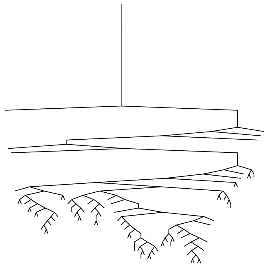
We have thus turned to the recursive method. Using the Maple package Combstruct, we have been able to generate quickly enough lambda-terms of size 200 and unary height bounded by 200–which means that there is de facto no restriction on the unary height of the lambda-term. Figure 5 shows what can be considered as a “generic” lambda-term for this size.

Both classes, the one with bounded unary height and the one where all bindings have bounded unary length, can be used to approximate generic lambda-terms. But unfortunately, also in the case of bounded unary length of bindings we are facing the same difficulties when trying to generate them with a Boltzmann sampler. The probabilities for generating leaves, unary and binary nodes looks very similar to Figure 4. This fact can be explained as follows: For both classes of restricted lambda terms, the dominant radicand is either close or equal to the innermost radicand. But the Boltzmann sampler generates these from outside inwards. That is meant in the following sense: Each square-root is the analytical analogue of the lifting from one unary level to the next one (cf. (18) and (19) in order to see this). The Boltzmann sampler builds an object by starting from the root and attaching more and more nodes. So, the head of the term, i.e. the subtree comprising all nodes of unary height zero, is precisely the object corresponding to the outermost root; and this is generated before the nodes with larger unary height. But note that the generating function of the class of heads has a larger dominant singularity. Hence the tuning parameter of the Boltzmann sampler is far away from this singularity, thus giving the sampler a strong bias towards stopping. On the other hand, moving the parameter into an interval where the sampler works efficiently means that it is outside the domain of analyticity of the generating function associated with lambda-terms. This implies that we have a positive probability that the sampling process never stops. So the sampler becomes even more inefficient than with the badly chosen tuning we had before moving it to the allegedly better region. Bodini et al. [11] developed a general framework for Boltzmann sampling for which tuning parameters outside the region of convergence of the associated generating function can be used. This relies on anticipated rejection and might help to improve the Boltzmann samplers for generating random lambda-terms.

For restricted Motkzin trees the situation is totally different, because the dominant singularity comes from the outermost radicand. Thus the Boltzmann sampler starts to generate the object by generating subobjects corresponding to the root which determines the singularity, and we can choose the tuning parameter so that it in the optimal region.

8.2 Shape of a typical lambda-term

Being able to draw repeatedly random lambda-terms allows us to make tentative conjectures on their various parameters: profile, height, etc.

We have plotted in Figure 6 the ratio between the number of lambda-terms with unary height exactly $k$ and size $n$ , and the number of lambda-terms of size $n$ (without restriction on the height). The figure suggests that, for any given size $n$ , the unary height is close to a Gaussian distribution. In particular, this gives some experimental explanation to the change of difficulty which we encountered when generating terms of small unary height (size about 10 000, unary height bounded by 8) and terms of fairly large unary height (size about 10 000, unary height bounded by 135): The wave indicates the “good” estimate for the number of abstractions in a lambda-term; for instance, if we consider lambda-terms of size 198, then the vast majority of these terms has a unary height between 25 and 50.

Figure 5 shows a generic lambda-term, its profile (number of nodes at each level) and the profile averaged on 500 random lambda-terms, together with the average profile of a plane binary tree, which is up to scaling identical with that of Motzkin trees since both tree classes are simply generated. From our simulations we can make several empirical observations:

•

The distribution of the profiles is poorly concentrated (this is also the case for plane binary trees).
•

The levels containing the larger number of nodes are much farther from the root than in plane binary trees.
•

A simulation of the distribution for the total (unary) height also shows a clear difference to plane binary trees: The average (unary) height seems to grow almost linearly (actually proportional to $n/\log n$ ), not proportional to $\sqrt{n}$ as the height of binary trees or the unary height (and also the height) of Motzkin trees. Accordingly, the width of lambda-terms appears to grow as $\log n$ .
•

A random lambda-term usually begins with a large number of successive unary nodes interspersed with a few binary nodes; most binary nodes appear further down.

Figure 3 shows the underlying Motzkin tree of a large lambda term of bounded unary height (the bound is 8) and its profile. Simulations for the case of bounded unary length of binding lead to similar pictures. Certainly, one of the reasons is that the bound 8 is still very small to exhibit a visible qualitative difference between the two classes of lambda-terms. On the other hand, it is also possible that the shape of the underlying Motzkin tree is too similar in both models if $k$ is relatively small.

In contrast to this is the behaviour of Motzkin trees of bounded unary height. As Figure 7 shows, the position of most of the unary nodes seems to be near the leaves whereas in a random lambda-term of bounded unary height most the unary nodes form a string starting at the root (cf. Figure 5).

9 Conclusion and perspectives

In this paper we have studied several classes of lambda-terms; see also [6] for further classes. It is clear that allowing pointers from unary nodes to leaves is the main factor that determines the complexity of such structures, and the more unary nodes we allow, the farther we are from trees. Indeed, allowing pointers from internal nodes to leaves amounts to leaving the realm of trees for that of directed acyclic graphs. As regards the enumeration of restricted classes, bounding the number of unary nodes as well as bounding the unary length of bindings (which is locally bounding the number of levels of nesting for abstractions) leads to an asymptotic behaviour that resembles that of trees (of type $n^{-3/2}\rho^{n}$ ), even though the latter is already of considerable combinatorial complexity. In contrast, bounding the unary height (which means globally bounding the number of levels of nesting for abstractions) exhibits an unusual behaviour.

Among other facts, we have discovered the unexpected behaviour of the position of the dominant radicand, which jumps according to some function behaving as $\log(\log(k))$ , with $k$ being the bound for the unary height of a lambda-term. Theorem 3 characterizes precisely these jumps and the asymptotic number of lambda-terms with bounded unary height. The enumerative result looks tree-like unless the bound for the unary height belongs to the special sequence $(N_{j})_{j\geq 1}$ .

The fact that the generating function has a nested square-root representation, but the position of the dominant radicand depends on the specific restriction appeared also in our studies of Motzkin. We studied them for comparison reasons since they form the underlying structure of lambda-terms. Regarding the asymptotic enumeration results, they exhibit the tree-like pattern, except if we impose a very unnatural shape: In the case where all leaves have to be at the same unary height we observe a different singularity of different type. In this case all radicands are dominant, as opposed to the other cases where either the innermost or the outermost radicand is dominant.

In contrast to this stands the behaviour of lambda terms of bounded unary height where the position of the dominant radicand is depending on the bound for the unary height. This phenomenon requires further explanation.

Further investgations indicate that the strange jumps in the behaviour are related to the distribution of the leaves in a lambda-term with bounded unary height. It seems that they are concentrated in the last few levels (level counting w.r.t. unary height) while the lower levels contain almost no leaves. The number of these levels seems to be doubly logarithmic in the size of the terms and whenever $k=N_{j}$ for some $j$ , then a new level “enters”, meaning that it contains then a significant number of leaves. So, the special values of $k$ are those where a transition takes place from $\ell$ to $\ell+1$ levels, filled with almost all the leaves of the lambda-term. In lambda-terms belonging to the class where all bindings have bounded unary length we expect that the distribution of the different types of nodes (unary, binary and leaves) is more uniformly distributed within their underlying Motzkin trees than in the bounded unary height case. This is indicated by generation of small objects (size 100-200, cf. Figure 9).

A byproduct of our work concerns Boltzmann samplers: By trying to use them for the random generation of lambda-terms, we have pushed them to their limit. It turned out that Boltzmann samplers have serious difficulties to generate generic lambda-terms of large size. The same is true if the unary height or the length of the bindings is bounded. From an analytic view point, the reason is certainly that the dominant singularity does come from radicands lying in a deep level of nestings. Another reason might be that the multiplicative constants in the asymptotic main terms decrease so rapidly with growing $k$ . We analyzed these constants exhaustively for the case with bounds on the binding length, and for $k=N_{j}$ in the bounded unary height case. It remains an open problem to carry out a precise analysis for all $k$ and to understand those irregularities discussed in Section 7. We feel that it might be also possible to improve Boltzmann random generation, when we wish to apply it to combinatorial structures for which Boltzmann samplers mostly produce either small or infinite objects. Recently, a framework for Boltzmann sampling has been developed by Bodini et al.[11] which generalizes the existing one in a direction which might help to overcome some of the difficulties we are facing in the generation of lamda-terms.

We next mention that our approach can be extended to study formulas of quantified logic: Instead of a single type of unary nodes, we have as many types as different quantifiers (usually two: $\forall$ and $\exists$ ; $l$ in general). We also have as many types of binary nodes as there are binary connectors (e.g., two when we consider the connectors $\wedge$ and $\vee$ ; $h$ in general); here we have studied the case $l=h=1$ . We expect that allowing different types of unary nodes will introduce only a multiplicative coefficient in our results, whereas allowing different types of binary nodes will change the singularities and thus the exponential growth.

Finally, in terms of average properties and growth, lambda-terms widely differ from the usual models for trees such as simple families [40] or increasing trees [4], for which we know the behaviour of classical parameters: number of trees of given size, profile, etc. Indeed they seem to behave, in some sense, like “ornamented” paths, i.e. long strings onto which relatively small subterms are grafted.

Of course, such results need to be explained and quantified more rigorously. Let us also mention that the enumeration of (unrestricted) lambda-terms is still an open problem, which has to be solved in order to study such parameters as the (average) unary height, the profile, etc.

An interesting question is the probability that a random lambda-term is in normal form. We are currently studying this problem for restricted classes of lambda-terms and hope to give results in a forthcoming paper.

Acknowledgement .

The authors thank Pierre Lescanne for pointing out reference [47].

References

[1] Alfred V. Aho and Neil J. A. Sloane. Some doubly exponential sequences. Fibonacci Quarterly, 11:429–437, 1970.
[2] Cyril Banderier and Michael Drmota. Formulae and asymptotics for coefficients of algebraic functions. Combin. Probab. Comput. 24(1):1–53, 2015.
[3] Henk P. Barendregt. The Lambda Calculus Its Syntax and Semantics. Volume 103 of Studies in Logic and the Foundations of Mathematics. North-Holland Publishing Co., Amsterdam, revised edition, 1984.
[4] François Bergeron, Philippe Flajolet, and Bruno Salvy. Varieties of increasing trees. In CAAP ’92 (Rennes, 1992), volume 581 of Lecture Notes in Comput. Sci., pages 24–48. Springer, Berlin, 1992.
[5] Olivier Bodini, Danièle Gardy, and Bernhard Gittenberger. Lambda terms of bounded unary height. $7^{th}$ Workshop on Analytic Combinatorics (ANALCO), San Francisco (USA), January 2011. Proceedings in http://www.siam.org/proceedings/analco/2011/analco11.php, 23–32.
[6] Olivier Bodini, Danièle Gardy, Bernhard Gittenberger and Alice Jacquot. Enumeration of generalized BCI lambda-terms. Electronic Journal of Combinatorics, 20 (2013), article P30, 23 pages (electronic).
[7] Olivier Bodini, Danièle Gardy, and Alice Jacquot. Asymptotics and random sampling for BCI and BCK lambda terms. Theoret. Comput. Sci., 502:227–238, 2013.
doi: 10.1016/j.tcs.2013.01.008.
[8] Olivier Bodini, Danièle Gardy, and Olivier Roussel. Boys and girls birthdays and Hadamard products. Fundamenta Informaticae, special issue on Lattice Path Combinatorics and Applications, Vol. 117 (14), pp. 85–101, 2012.
[9] Olivier Bodini and Bernhard Gittenberger. On the asymptotic number of BCK(2)-terms. ANALCO14-Meeting on Analytic Algorithmics and Combinatorics, SIAM, Philadelphia, PA, 25–39, 2014.
[10] Olivier Bodini and Alice Jacquot. Boltzmann samplers for colored combinatorial objects. $6^{th}$ GASCOM workshop, Bibbiena (Italy), June 16–19, 2008.
[11] Olivier Bodini, Jérémie Lumbroso, and Nicolas Rolin. Analytic samplers and the combinatorial rejection method. In Proceedings of the Twelfth Workshop on Analytic Algorithmics and Combinatorics, ANALCO 2015, San Diego, CA, USA, January 4, 2015, pages 40–50, 2015.
[12] Olivier Bodini and Yann Ponty. Multi-dimensional Boltzmann sampling of languages, Conference on Analysis of Algorithms, AofA’10, Vienna (Austria), June 28-July 2, 2010. DMTCS Proceedings, AM, 49–64, 2010.
[13] Manuel Bodirsky, Eric Fusy, Mihyun Kang, and Stefan Vigerske. Boltzmann samplers, Polya theory, and cycle pointing, SIAM Journal on Computing, 40(3):721–769, 2011.
[14] Miklós Bóna and Philippe Flajolet. Isomorphism and symmetries in random phylogenetic trees, Journal of Applied Probability, 46:1005–1019, 2009.
[15] Jérémie Bouttier and Emmanuel Guitter. Planar maps and continued fractions, Comm. Math. Phys., 309:623–662, 2012.
[16] Alonzo Church. An unsolvable problem of elementary number theory. Amer. J. Math., 58(2):345–363, 1936.
[17] G. Darboux. Mémoire sur l’approximation des fonctions de très-grands nombres, et sur une classe étendue de développements en série. J. Math. Pures Appl. (3. Série), 4:5–56, 377–416, 1878.
[18] René David, Katarzyna Grygiel, Jakub Kozik, Christophe Raffalli, Guillaume Theyssier, and Marek Zaionc. Asymptotically almost all $\lambda$ -terms are strongly normalizing. Log. Methods Comput. Sci., 9 (2013), no. 1, 1:02, 30 pp.
[19] René David and Marek Zaionc. Counting proofs in propositional logic. Arch. Math. Logic, 48(2):185–199, 2009.
[20] Michael Drmota. Random trees. SpringerWienNewYork, Vienna, 2009. An interplay between combinatorics and probability.
[21] Philippe Duchon, Philippe Flajolet, Guy Louchard, and Gilles Schaeffer. Boltzmann samplers for the random generation of combinatorial structures, Combinatorics, Probablity, and Computing, 13:(4-5):577–625, 2004. Special issue on Analysis of Algorithms.
[22] Philippe Flajolet. Combinatorial aspects of continued fractions, Discrete Mathematics, 32:125–161, 1980. Reprinted in the 35th Special Anniversary Issue of Discrete Mathematics, Volume 306, Issue 1011, Pages 992–1021 (2006).
[23] Philippe Flajolet, Eric Fusy, and Carine Pivoteau. Boltzmann sampling of unlabelled structures, Proceedings of ANALCO’07 (Analytic Combinatorics and Algorithms), SIAM Press, ed., vol. 126, 2007, pp. 201–211.
[24] Philippe Flajolet and Andrew Odlyzko. Singularity analysis of generating functions. SIAM Journal on Discrete Mathematics, 3(2):216–240, 1990.
[25] Philippe Flajolet and Robert Sedgewick. Analytic combinatorics. Cambridge University Press, Cambridge, 2009.
[26] Philippe Flajolet, Paul Zimmerman, and Bernard Van Cutsem. A calculus for the random generation of labelled combinatorial structures, Theoret. Comput. Sci., 132(1-2):1–35, 1994.
[27] Hervé Fournier, Danièle Gardy, Antoine Genitrini, and Bernhard Gittenberger. The fraction of large random trees representing a given Boolean function in implicational logic. Random Structures and Algorithms, 40(3):317–349, 2012.
[28] Antoine Genitrini, Jakub Kozik, and Marek Zaionc. Intuitionistic vs. classical tautologies, quantitative comparison. In Types for proofs and programs, volume 4941 of Lecture Notes in Comput. Sci., pages 100–109. Springer, Berlin, 2008.
[29] R.L. Graham, D.E. Knuth and O. Patashnik. Concrete Mathematics. Addison-Wesley, 1994.
[30] K. Grygiel and P. Lescanne. Counting terms in the binary lambda calculus. J. Funct. Programming, 23(5):594–628, 2013.
[31] J. Roger Hindley. BCK and BCI logics, condensed detachment and the $2$ -property. Notre Dame J. Formal Logic, 34(2):231–250, 1993.
[32] Yasuyuki Imai and Kiyoshi Iséki. Corrections to: “On axiom systems of propositional calculi. I”. Proc. Japan Acad., 41:669, 1965.
[33] Yasuyuki Imai and Kiyoshi Iséki. On axiom systems of propositional calculi. I. Proc. Japan Acad., 41:436–439, 1965.
[34] Kiyoshi Iséki and Shôtarô Tanaka. An introduction to the theory of BCK-algebras. Math. Japon., 23(1):1–26, 1978/79.
[35] Stephen C. Kleene. A theory of positive integers in formal logic. Part I. Amer. J. Math., 57(1):153–173, 1935.
[36] Stephen C. Kleene. A theory of positive integers in formal logic. Part II. Amer. J. Math., 57(2):219–244, 1935.
[37] P. J. Landin. A correspondence between ALGOL 60 and Church’s lambda-notation. I. Comm. ACM, 8:89–101, 1965.
[38] P. J. Landin. A correspondence between ALGOL 60 and Church’s lambda-notation. II. Comm. ACM, 8:158–165, 1965.
[39] Pierre Lescanne. On counting untyped lambda terms. Theoret. Comput. Sci. 474:80–97, 2013.
[40] A. Meir and J. W. Moon. On the altitude of nodes in random trees. Canadian Journal of Mathematics, 30:997–1015, 1978.
[41] Albert Nijenhuis and Herbert S. Wilf. Combinatorial Algorithms. Academic Press, 1978.
[42] Richard Otter. The number of trees, Ann. of Math. 49 (3):583–599, 1948.
[43] Carine Pivoteau, Bruno Salvy, and Michèle Soria. Algorithms for combinatorial structures: Well-founded systems and Newton iterations. Journal of Combinatorial Theory (A), 119(8):1711–1773, 2012.
[44] Olivier Roussel and Michèle Soria. Boltzmann sampling of ordered structures. Electronic Notes in Discrete Mathematics, 35:305–310, 2009.
[45] Morten Heine Sørensen and Paweł Urzyczyn. Lectures on the Curry-Howard Isomorphism. Amsterdam: Elsevier, 2006.
[46] W. T. Tutte. The number of planted plane trees with a given partition. Amer. Math. Monthly, 71:272–277, 1964.
[47] Xuejun Yang, Yang Chen, Eric Eide, and John Regehr. Finding and understanding bugs in C compilers. ACM SIGPLAN Notices - PLDI ’11, 46(6):283–294, 2011.
[48] Marek Zaionc. On the asymptotic density of tautologies in logic of implication and negation. Reports on Mathematical Logic, 39:67–87, 2005.

	$\displaystyle\|x\|$	$\displaystyle=1,$
	$\displaystyle\|\lambda x.T\|$	$\displaystyle=1+\|T\|,$
	$\displaystyle\|(S*T)\|$	$\displaystyle=1+\|S\|+\|T\|.$

On the number of unary-binary tree-like structures with restrictions on the unary height

Abstract

1 Introduction

2 A combinatorial description for lambda-terms

2.1 Representation as directed acyclic graphs

Definition 1.

Definition 2.

2.2 Generating functions associated with lambda-terms

Remark 1.

Definition 3.

Definition 4.

Remark 2.

3 Restricted Motzkin trees

3.1 Restrictions on the total number of unary nodes

Proposition 1.

Proof.

Lemma 1.

Proof.

3.2 Restrictions on the unary height

3.2.1 All leaves at the same unary height

Lemma 2.

Proposition 2.

Remark 3.

3.2.2 Motzkin trees of bounded unary height

Lemma 3.

Lemma 4.

Proof.

Remark 4.

Proposition 3.

4 Enumeration of lambda-terms with prescribed number of unary nodes

4.1 Recurrence for the generating functions

4.2 Solving the recurrence

Lemma 5.

Proof.

Lemma 6.

4.3 Asymptotics

Proposition 4.

Remark 5.

4.4 Lambda-terms with at most qq unary nodes

5 Enumeration of lambda-terms with bounded unary length of bindings

5.1 Analysis of the radicands

Definition 5.

Lemma 7.

Proof.

Lemma 8.

Proof.

Lemma 9.

Proof.

Proposition 5.

Proof.

Theorem 1.

Proof.

5.2 Asymptotic decrease of constant term

Proposition 6.

Lemma 10.

Proof.

6 Enumeration of lambda-terms of bounded unary height

6.1 Analysis of the radicands

Definition 6.

Corollary 1.

Proof.

Remark 6.

Theorem 2.

6.1.1 The radicands Ri,kR_{i,k}

6.1.2 The dominant singularity of a radicand

Lemma 11.

Proof.

Corollary 2.

Remark 7.

Definition 7.

Lemma 12.

Proof.

Lemma 13.

Proof.

Lemma 14.

Proof.

6.1.3 When two successive radicands vanish

Lemma 15.

Proof.

Remark 8.

4.4 Lambda-terms with at most $q$ unary nodes

6.1.1 The radicands $R_{i,k}$

6.1.4 The sequence $(N_{i})_{i\geq 1}$

6.3 The location of singularities for large $k$

6.4.1 The derivative of $R_{j,k}(z)$

6.4.2 Asymptotic expansion of $\prod_{i=1}^{M}{\lambda_{i}}$ .

Acknowledgement .