Boosting in the presence of outliers:
adaptive classification with non-convex loss
functions
Abstract
This paper examines the role and efficiency of the non-convex loss functions for binary classification problems. In particular, we investigate how to design a simple and effective boosting algorithm that is robust to the outliers in the data. The analysis of the role of a particular non-convex loss for prediction accuracy varies depending on the diminishing tail properties of the gradient of the loss – the ability of the loss to efficiently adapt to the outlying data, the local convex properties of the loss and the proportion of the contaminated data. In order to use these properties efficiently, we propose a new family of non-convex losses named -robust losses. Moreover, we present a new boosting framework, Arch Boost, designed for augmenting the existing work such that its corresponding classification algorithm is significantly more adaptable to the unknown data contamination. Along with the Arch Boosting framework, the non-convex losses lead to the new class of boosting algorithms, named adaptive, robust, boosting (ARB). Furthermore, we present theoretical examples that demonstrate the robustness properties of the proposed algorithms. In particular, we develop a new breakdown point analysis and a new influence function analysis that demonstrate gains in robustness. Moreover, we present new theoretical results, based only on local curvatures, which may be used to establish statistical and optimization properties of the proposed Arch boosting algorithms with highly non-convex loss functions. Extensive numerical calculations are used to illustrate these theoretical properties and reveal advantages over the existing boosting methods when data exhibits a number of outliers.
1 Introduction
Recent advances in technologies for cheaper and faster data acquisition and storage have led to an explosive growth of data complexity in a variety of research areas such as high-throughput genomics, biomedical imaging, high-energy physics, astronomy and economics. As a result, noise accumulation, experimental variation and data inhomogeneity have become substantial. Therefore, developing classification methods that are highly efficient and accurate in such settings, is a problem that is of great practical importance. However, classification in such settings is known to poses many statistical challenges and calls for new methods and theories. For binary classification problems, we assume the presence of separable, noiseless data that belong to two classes and in which an adversary has corrupted a number of observations from both classes independently. There are a number of setups that belong to this general framework. A random flipped label design, in which the labels of the class membership were randomly flipped, is one example that can occur very frequently, as labeling is prone to a number of errors, human or otherwise. Another example is the presence of outliers in the observations, in which a small number of observations from both classes have a variance that is larger than the noise of the rest of the observations. Such situations may naturally occur with the new era of big and heterogeneous data, in which data are corrupted (arbitrarily or maliciously) and subgroups may behave differently; a subgroup might only be one or a few individuals in small studies that would appear to be outliers within class data.
Considerable effort has therefore been focused on finding methods that adapt to the relative error in the data. Although this has resulted in algorithms, e.g. Grünwald and Dawid (2004), that achieve provable guarantees (Natarajan et al., 2013; Kanamori et.al, 2007) when contamination model (Scott et al., 2013) is known or when multiple noisy copies of the data are available (Cesa-Bianchi et al., 2011), good generalization errors in the test set are by no means guaranteed. This problem is compounded when the contamination model is unknown, where outliers need to be detected automatically. Despite progress on outlier-removing algorithms, significant practical challenges (due to exceedingly restrictive conditions imposed therein) remain. In this paper, we concentrate on the ensemble algorithms. Among these, AdaBoost (Freund and Schapire, 1997) has proven to be simple and effective in solving classification problems of many different kinds. The aesthetics and simplicity of AdaBoost and other forward greedy algorithms, such as LogitBoost (Friedman, et al., 2000), also facilitated a tacit defense from overfitting, especially when combined with early termination of the algorithm (Zhang and Yu, 2005). Friedman, et al. (2000) developed a powerful statistical perspective, which views AdaBoost as a gradient-based incremental search for a good additive model using the exponential loss. The gradient boosting (Friedman, 2001) and AnyBoost (Mason et al., 1999) have used this approach to generalize the boosting idea to wider families of problems and loss functions. This criterion was motivated by the fact that the exponential loss is a convex surrogate of the hinge or loss. Nevertheless, in the presence of label noise and/or outliers, the performance of all of them deteriorates rapidly (Dietterich, 2000). Although algorithms like LogitBoost, MadaBoost (Domingo and Watanabe, 2000), Log-lossBoost (Collins, et al., 2002) are able to better tolerate noise than AdaBoost, they are still not insensitive to outliers. Hence, they are efficient when the data is observed with little or no noise. However, Long and Servedio (2010) pointed out that any boosting algorithm with convex loss functions is highly susceptible to a random label noise model. They constructed a simple example, from hereon denoted Long/Servedio problem, that cannot be “learned” by the boosting algorithms above.
Center to our analysis is the work by Freund (2009). He proposed a robust boosting algorithm based on the Boost by majority (BBM) (Freund, 1995) and BrownBoost (Freund, 2001) algorithm, which uses a non-convex loss function. Instead of maximizing the margin, the algorithms achieve robustness by allowing a preassigned error of margin maximization (Servedio, 2003). Moreover, in each step, the algorithms update and solve a differential equation and update the preassigned remaining time or the target error . As the loss function changes with each iteration of the algorithm, they do not agree with the general boosting interpretation through additive models. Furthermore, with at least two preassigned parameters, each of them is difficult to implement and is highly inconsistent with respect to minor changes in the settings. Surprisingly, statistical and convergence properties of these two algorithms are still unknown. This leads to a natural question: how do we develop a simple but effective boosting algorithm that has a non-convex loss function, that preserves boosting interpretation and that is robust to the noise in the data? In this paper, we address this question and propose a fully automatic estimator, with no tuning parameters to be chosen, that has provable guarantees.
To design the new framework we will explore and amend the drawbacks of the AdaBoost algorithm in the contaminated data setting. We successfully identify that the AdaBoost’s sensitivity to outliers comes from the unbounded weight assignment of the misclassified observations. As outliers are more likely to be misclassified, they are very likely to be assigned large weights and will be repeatedly refitted in the following iterations. This refitting will deteriorate seriously the generalization performance of the algorithm, as the algorithm “learns” incorrect data distribution. To achieve robustness, the algorithm should be able to abandon observations that are on the extreme, incorrect side of the boundary. Here, we theoretically and computationally investigate the applicability of non-convex loss functions for this purpose. We illustrate that the best weight updating rule is to assign a weight of to each data point , in which is the appropriate non-convex loss function. We use a tilting argument, with non-convex losses. It is shown that, if we use a non-convex loss, sufficiently tilted, i.e. such that is small for all , then the outliers are eliminated successively. Hence, constant tilting or “trimming” is not sufficient for outlier removal. In tilting the loss function, we are effectively preserving as much fidelity to the data as possible, while redistirbuting emphasis to different observations. We propose a new Arch Boosting framework that implements the above tilting method and adjusts for optimality by a new search of the optimal weak hypothesis. Moreover, we show that the new framework avoids overfitting much similar to the AdaBoost. We propose a sufficient set of conditions needed for a loss function to allow for good properties of the ArchBoost. We show that not every non-convex function satisfies such conditions; an example is the sigmoid loss. However, we propose a family of loss functions that balances both the benefits of non-convexity and the empirical risk interpretation of boosting.
Properties of the boosting algorithms based on convex loss functions have been extensively studied (e.g. Koltchinskii and Panchenko (2002); Zhang and Yu (2005)). Comparatively little is known for the non-convex losses, as the existing techniques do not apply. We show that local convexity properties are sufficient for statistical consistency. Furthermore, even though the proposed loss function is shown to enjoy the aforementioned local convexity, it is largely unknown whether numerical algorithms can identify this local minimizer. Moreover, as our algorithm is not defined as a gradient descent algorithm, we require a new approach for the proof of numerical convergence. We develop a new sufficient optimality condition based on the “hardness condition” in the technical proofs. By hardness property, we mean the orthogonality of the new reweighted classifier and the class membership vector. Furthermore, we address the robustness and efficiency of the proposed method, with respect to the outliers. Although it is straightforward to provide such analysis for parametric linear models, computations for classification with the nonparametric boundaries are far more challenging. We provide a novel analysis, for which we propose a new finite sample breakdown point theory (Hampel, 1968) and show that the influence function (Hampel, 1974) is bounded for appropriate class of classification problems. To the best of our knowledge, this is the first result regarding the robustness properties of the boosting algorithms, with respect to the presence of outliers. Our analysis allows for both convex and non-convex loss function. We finalize the analysis with a proof of statistical consistency of the proposed method that includs many non-convex losses; we do so by exploring local curvatures of the loss.
In essence, this paper investigates the effects of non-convex losses on a variety of boosting algorithms in the presence of unknown contamination of the data. In particular, we focus on how to design a new boosting framework in order to improve the prediction accuracy of classification methods for the data with outliers. The rest of the paper is organized as follows. We present a new Arch boosting framework in Section 2; it is designed for augmenting the boosting framework such that its corresponding classification algorithm is significantly more adaptable to outliers. Section 3 outlines a new family of loss functions that explores non-convexity and present sufficient conditions for non-convex loss to be robust. We present theoretical analysis in Section 4: the numerical and statistical convergence of the proposed algorithms are discussed in 4.1 and 4.3, respectively. Moreover, we show theoretical robust properties in the Section 4.2 with the breakdown point discussed in Section 4.2.2 and influence function in Section 4.2.3. Section 5 contains numerical experiments on a number of examples of the loss functions belonging to the introduced family: -robust loss, least squares, logistic, exponential and truncated exponential loss. We demonstrate both how to use these methods in practice and compare them to the alternative of applying the non-augmented AdaBoost algorithm to the noisy data. The subsection 5.1 varies the parameter and considers examples of a contaminated Gaussian distribution. All examples clearly illustrate that the methods outlined in Section 3 are far more successful than the existing boosting methods. Section 5.2 deals with the more complex situation of Long/Servedio data for which we show that our Arch Boost method outperforms the robust boosting method of Freund (2009). We also discuss outlier detection examples in Section 5.3, and apply our methods to three real datasets in Section 5.4.
2 Arch Boost
We consider a binary classification problem, with denoting the domain of the -dimensional variable , and denoting the class label set that equals . We aim to estimate a function and assume that the training data are i.i.d. copies of with unknown distribution. The data consists of samples from the contaminated distribution that is composed of the true (uncontaminated) data and a fixed and unknown number of outliers in each of the classes.
From now on, we let denote any differentiable loss function. Note that does not need to be convex necessarily. For such , we define the risk and the empirical risk as
| (1) |
where is the sample size, are i.i.d observations, and is the true probability distribution on . For simplicity of notation, we write . Note that the observed samples can come from a contaminated distribution, i.e., they are i.i.d. samples from for small, but positive contamination .
We view boosting as a method that iteratively builds an additive model,
where belongs to a large (but we will assume finite VC-dimension) space of weak hypotheses, denoted with . The use of our framework in the presence of countably infinite features, also known as the task of feature induction, can easily be established. Next, we introduce the new framework of the boosting in the presence of the noise, which we call an Arch Boosting framework.
We design the Arch Boosting framework as a stage-wise, iterative, minimization of the -risk (1). However, when is non-convex this cannot be done by simply applying the well known Friedman’s Gradient Boosting (Friedman, 2001). The explicit updates are usually unavailable and standard numerical methods like Newton-Raphson, which are suitable only for convex functions, are used. Instead, we constrain the stage-wise minimization of the -risk to keep one additional important property of the boosting algorithms, namely the hardness condition of Freund and Schapire (1997). It is shown that hardness condition can easily distinguish between the outliers and the center of the data, when non-convex loss is used. Moreover, it allows for a fine tuning of the appropriate optimal hypothesis assignments such that the minimization of the -risk is approximately kept. Therefore, hardness condition allows us to simultaneously escape the non-convexity in the minimization and to use non-convexity to separate the outliers from the inliers. This property, from iteration to , is defined as
| (2) |
where is defined as a weighted conditional expectation
| (3) |
The equation (2) can be explained as progressing from step to ; the weights are updated from to , such that is orthogonal to with respect to the inner product defined on the reweighed data . In a certain sense, the weights are chosen as the most difficult for the weak hypothesis . For the weight vector the hypothesis is not better than a random guess.
Recall that our goal is to find the optimal , which minimizes the -risk for a suitable class of measurable functions . In the binary case, each instance is associated with a label and the goal of learning is then to find a classifier , such that the sign of is equal to . In order to minimize , we minimize it at every point – that is, given any , considering as a parameter and denoting , the problem is to find
| (4) |
Table 1 contains a list of commonly used loss functions and the corresponding optimal classifiers when , which is the family of all measurable functions.
| Classification Method | Population parameters | ||
|---|---|---|---|
| Loss function | Optimal Minimizer | ||
| Logistic | |||
| Exponential | |||
| Least Squares | |||
| Modified Least Squares | |||
Provided that and for any , has only one critical point at that is the global minimum, we can find by the first order optimality condition
| (5) |
Expanding on the above first order optimality conditions, we obtain
where is defined as the first order derivative . In classification problems, the input of loss function is – that is, the margin of a classifier applied to a data point . Rewriting the expectation in terms of the class probabilities, we obtain the following representation of the first order optimality conditions
| (6) |
From now on, without confusion, we write instead of . We aim to mimic equation ebove in each of the iteration steps of the proposed framework. In more details, at iteration , with the current estimate at hand, we wish to find a new weak hypothesis , such that with that solving the following equation
| (7) |
If we can always accurately find such a weak hypothesis (i.e. is rich enough and we know the true distribution), then this process will terminate in just one step. However, complications arise from two aspects. First, we only have a restricted family of weak hypotheses. Therefore, at each iteration, an approximated weak hypothesis, which is the closest approximation in , will be found. Secondly, the equation (7) alone cannot be efficiently utilized since , which is the ultimate goal of classification problems, is unknown to us. However, we propose to solve approximated equation, where we replace with the weighted conditional probability at each iteration of the proposed algorithm. Hence, with the weighted conditional expectation defined in (3).
In more details, at each iteration , for a given , we find such that it solves the estimating equation
| (8) |
for a suitable function to be specified later. In order to do this, we will first discuss how to define the weights at each iteration and postpone the method of finding for later.
Since is only an approximation to the optimal increment at step , instead of adding itself to we multiply it by a constant and search for the best constant . The best should be such that the updating classifier approaches the optimal one, defined in equation (6). Hence, we define the optimal as the solution to the following optimization problem
| (9) |
Similarly to the AdaBoost, at each iteration , the data will be reweighed according to the weights . We explore relation (9) further to find the optimal weights . For that purpose, we observe that for a given (from a previous iteration) and (solving (8)) the optimal then satisfies
| (10) |
Then, we recall the hardness condition of the AdaBoost algorithm: the weights should be updated such that the weighted misclassification error of the most recent weak hypothesis is about . According to (2), this can be achieved by defining the weights such that
| (11) |
Now, in the Arch Boost framework the most recent weak hypothesis is . Hence, by contrasting the last two equations, (10) and (11), we define the weights to be
such that both the hardness condition and the optimality of the updating hypothesis are satisfied.
Having defined the weight updating rule, we go back to equation (7) to define the optimal weak hypothesis . We do so by finding a relationship between and and defining the function of (8). We multiply (7) with on both sides to obtain
| (12) |
Then, it is easy to observe that
Hence, we have
| (13) |
that is, equation (8) is true for
Observe that the right hand side of (13) can be estimated by a weak learner at each iteration . For reference, we list the weak hypothesis for several commonly used loss functions in the Table 2.
| Classification Method | Population parameters | ||
| Loss function | Optimal weak hypotheses | ||
| Logistic | |||
| Exponential | |||
| Least Squares | |||
| Modified Least Squares | |||
| * | |||
Note that the weak hypotheses of the least squares loss and modified least squares loss depend on the current estimate and the weighted conditional probability , which is different from that of Gradient boosting (Friedman, 2001). Lastly, we summarize the above procedure in the following Algorithm 1, which we call Arch Boost. The assumption that has only one critical point does not require the loss function to be convex and hence the Arch Boost algorithm can be applied to many non-convex loss functions. We illustrate this in Section 3 by proposing a family of robust boosting algorithms based on the Arch Boosting framework.
In the step (b) of the Algorithm 1, any classifier can be used; one example is a decision tree for which case is the proportion of the training samples with label in the terminal node, where ends up. For instance, in terminal region , let stands for the index set of data points with positive label, then .
Note that in the step , whenever , then can be or . In order to deal with this problem, one method is to only update the points with . If becomes infinity after some step , then we keep it to be infinity and do not update further. Finally, we just set and . Another method is simply applying a map to the class probability estimations where is a constant very close to 1 (e.g. ).
3 Robust boosting algorithms
In this section, we propose a new class of boosting algorithms especially designed to be resilient to the presence of extraneous noise in the data. Whether this noise comes in the forms of mislabeled data points, additional variance within class data, or malicious data, the proposed algorithm adapts to it with great success. We begin the section by proposing a new loss function, which we have named two-robust loss function. Furthermore, we characterize regularity conditions that a loss function needs to satisfy, in order to be appropriate for Arch Boosting framework. Finally, we provide a family of loss functions that is not convex and that satisfies the newly defined regularity conditions and the corresponding family of robust boosting algorithms called ARB-.
3.1 A non-convex loss
An approach of non-convex functions has been recognized as successful in the existing literature. Both Freund (2001) and Freund (2009) have utilized it to propose boosting methods that are resilient to the presence of outliers in the data. However, both loss functions require a number of tuning parameters. The behavior of the algorithm is hindered by the optimal choice of such parameters. Moreover, such optimal choices are data dependent and not isolated as universal by either approach.
Driven by the need to propose an alternative loss function that can be easily used in many situations, we propose the following non-convex loss function:
| (14) |
The proposed loss function (14) has optimal , the weak hypothesis, and the weight updating rule as presented in Table 3. We call the function (14) two-robust loss and it belongs to a family of loss functions that will be discussed in Section 3.3. By adopting the Arch Boosting framework of Algorithm 1 we illustrate the nice downweighting property of the new weight updating rule with this new loss function.
| Arch 2-boosting | Optimal parameters | |||
|---|---|---|---|---|
| Loss function | Optimal minimizer | Weak hypothesis | Weight vector | |
| Arch |
In Figure 1, we plot the two-robust loss (14), together with exponential and logistic regression losses and the corresponding weight updating rules.
We observe that the two-robust loss is non-convex and bounded from above when . Therefore, the outliers, even if large in size, will only have bounded influence on the classification. Moreover, by investigating the weight updating rule, we observe that the more misclassified the data point is, the smaller the weight updating function will be. The algorithm, in fact, abandons the data points that are repeatedly misclassified and are far from the Bayes boundary. This phenomenon disappears when one uses exponential loss or logistic loss and, in fact, any commonly used convex loss function. To the best of our knowledge, no existing loss function satisfies this nice property without requiring a-priori fixed tuning parameters. By plugging the two-robust loss into Arch Boost, we obtain new boosting algorithm that we named Adaptive Robust Boost-2, denoted with ARB-2 from hereon.

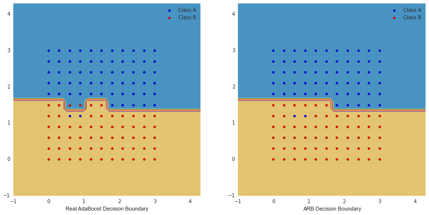
Next, we consider a simple two dimensional binary classification example consisting of two mislabeled points near the classification boundary. The example is artificially created to illustrate the point of an adaptive classifier, when there are outliers in the data. We evenly put 121 points in the region , that is, , where . For each , the corresponding if and otherwise. Then we flip the labels of and . The step sizes, , for both algorithms are set to be constant 0.5, and the number of iterations is set as . We show the difference between the Real AdaBoost and the ARB-2 in Figure 2. It can be seen that the decision boundary of AdaBoost are influenced by the two blue “abnormal” data points. But for ARB-2, the decision boundary stays the same as if there were no such abnormal points, hence it adapts to the outliers.
3.2 Loss functions for Arch Boost
In the previous section, we have seen an example of a robust boosting algorithm. Nevertheless, there are plenty of other non-convex functions which leads to the question: can we use any of them as a loss function for the Arch Boost? The answer is no, if we do not impose auxiliary conditions. In this section, we discuss what kinds of conditions need to be imposed so that a non-convex function becomes a suitable loss function for the Arch Boost framework 1.
Recall that in a binary classification problem, we want to minimize , to find
| (15) |
Since , the equation above becomes a convex combination of and . Therefore, one necessary condition on loss functions is that (15) has a unique optimal solution in . Observe that if is a class of all measurable functions, then can take any real value for every . This condition is not equivalent to the convexity of the loss function but rather to the local convexity around the true parameter of interest, . In the next section we present a family of non-convex loss functions that possess this property. Hence, we present the set of regularity conditions in the Definition below.
Definition 1.
A function is an Arch boosting loss function if it is differentiable and
- (i)
for all and ;
- (ii)
for any , has only one critical point which is the global minimum;
- (iii)
for any and , .
Conditions and together imply that is an upper bound of the - loss up to a constant scaling. Condition is a “classification calibration” (Bartlett et al., 2006) and is considered the weakest possible condition imposed on for which a measurable function which minimizes the risk will also have the risk close to the minimal one; in other words, close to that of the optimal that creates a Bayes boundary. If the function is convex, then condition is satisfied as long as is differentiable and . However, when considering non-convex losses, the set of regularity conditions doesn’t exists in the current literature. The above framework includes non-convex loss functions and differs from the existing literature on convex losses in that it includes an additional condition (see Section 4).
Lemma 1.
A positive function that is continuously differentiable, convex and such that is not equal to a constant satisfies Condition (ii).
By Lemma 1, we know that the logistic, the exponential, the least square and the modified least square loss are all Arch boosting loss functions. Differentiability of the loss function is a technical condition and is not crucial for the proposed framework. The hinge loss is not differentiable but can be shown to satisfy Conditions -. However, if we plug in the hinge loss to the equation (6), we cannot easily find the optimal solution . However, not every differentiable and non-convex loss function satisfies regularity conditions above.
Remark 1.
The sigmoid loss is differentiable and satisfies Condition (iii), but it does not satisfy Condition (ii) and hence is not an Arch Boosting loss function.
Finally, we provide a more general characterization for the loss functions, including not necessarily convex loss functions, which satisfy Condition .
Lemma 2.
Let be a positive, continuously differentiable loss function such that for all . Let , be defined as . Then satisfies Condition (ii) as long as function is a decreasing, bijection.
3.3 A family of non-convex functions and ARB- algorithms
Recall that the optimal classifier satisfies equation (6). We observe that the right hand side of this equation does not depend on the loss function and can take values in the positive real line, . Hence, we can parameterize it with any real-valued function whose range is , as follows
| (16) |
for any surjective, decreasing function . The classical motivation for reparametrization (McCullagh and Nelder, 1989) – often called link functions – is that often one uses a parametric representation that has a natural scale matching the desired one. We choose to use the function for any constant , which is a surjection. This parametrization is not unique but it admits a solution to the following differential equation
| (17) |
Solving it for (exact steps are presented in the Appendix A), we obtain a family of non-convex functions
| (18) |

Observe that parameters and are not tuning parameters, but rather an index set of a family of non-convex losses much like Huber and Tukey’s biweight losses are. Note that when , the right hand side of (17) can take all the real values and is monotonically increasing and consequently the corresponding loss will always give a unique solution to (6). We name each element in the family (18) as -robust loss function. Later, we will show that the positive parameter is irrelevant in our algorithms, so we can fix it to be . Note that for and , we obtain the non-convex loss function (14). Moreover, each loss function is a bounded function with upper bound equal to . Therefore, the effects of the outlier will be necessarily bounded. Moreover, the weight updating rule will also downweight the largely misclassified data points. We plot with different values and the corresponding normalized weight updating rules in the Figure 3. From Figure 3, we can see that for different , the peak point of each of the weight updating rules shifts to the left when increases. When , the weight updating curve is symmetric about and in fact, this is equivalent to the Sigmoid loss function when (Mason et al., 1999). Moreover, for and the loss is equivalent to the Savage loss function of Mesnadi-Shirazi and Vasconcelos (2009), in which they used the probability elicitation technique from Savage (1971) to design new loss functions.
Lemma 3.
For all , is an Arch Boosting loss function.
Lemma 3 allows us to plug with into the Arch Boost framework and obtain a family of robust boosting algorithms which we name Adaptive Robust Boost- (ARB-). The details are presented in the Algorithm 2 with computations relegated to the Appendix A.
| (19) |
4 Theoretical Considerations
Despite the substantial body of existing work on Gradient Boosting classifiers and AdaBoost in particular (e.g. Bartlett et al. (2006); Bartlett and Traskin (2007); Freund (1995); Friedman, et al. (2000); Schapire (1999); Schapire et al. (1998); Zhang and Yu (2005); Breiman (2004); Koltchinskii and Panchenko (2002)), research on robust boosting classifiers has mostly been limited to methodological proposals with little supporting theory (e.g., Gentile and Littlestone (1999); Kearns and Li (1993); Littlestone (1991)). However, whereas the loss functions studied in those papers are finite-sample versions of globally convex functions, many important robust classifiers, such as those arising in Freund (2009) and the proposed ARB-, only possess convex curvature over local regions even at the population level. In this paper, we present new theoretical results, based only on local curvatures, which may be used to establish statistical and optimization properties of the proposed Arch boosting algorithms, with highly non-convex loss functions.
4.1 Numerical convergence of Arch Boost algorithm
We show that the empirical risk will always decrease and that the Arch Boost can be viewed as the step-wise iterative minimization of the empirical risk . Similar results can be found in Koltchinskii and Panchenko (2002) and Zhang and Yu (2005). The main difference is that the authors use the gradient descent rule in the first or an approximate minimization in the second paper, while here we use the hardness condition to select the optimal weak hypothesis . We use to denote the weights on the data such that . Recall that for any classifier and any data point , the term always stands for the margin. For any weak hypothesis , we denote the expected margin as and the empirical margin as To introduce the notation used in the theorem, for any family of weak classifiers , we denote
| (20) |
a set of -combinations () of functions in . Let be a sequence of functions with empirical risk converging to , defined as . Then, can be represented as . In this respect, we define its norm as .
Theorem 1.
Assume is an Arch boosting loss function. Furthermore, assume that the weak learner is able to provide disjoint regions on the domain at each iteration (e.g. decision tree). We apply the Arch Boost () algorithm to a sample for iterations.
- (i)
If at each iteration the weak hypotheses satisfies , then will converge in as .
- (ii)
At each iteration , let be the set of disjoint regions on returned by the weak hypothesis , and be the class probability estimation in that region. If there exists a strictly increasing function with , and a positive constant such that satisfies the representation
for all , then .
- (iii)
Using any Arch boosting loss function for the Arch Boost Algorithm 1, at any iteration , there exists such a function that satisfies (ii).
- (iv)
Let be a sequence of functions with empirical risk converging to and such that
where and as . Furthermore, assume is Lipschitz differentiable, is bounded and as . Then, if a sequence of step sizes is such that
for a sequence of positive numbers , we have as .
Theorem 1 suggests that for any ARB- algorithm, the weak hypothesis at each iteration has a corresponding function that satisfies . Therefore, satisfies and with it, by , the ARB- algorithm converges when the number of iterations increases. The conditions in part (iv) are somewhat different compared to the equivalent one obtained for the gradient boosting with convex losses (Zhang and Yu, 2005). The reference sequence needs to be in a local neighboorhood of in the sence that cannot blow up too rapidly. Moreover, the size of cannot be smaller than implying that the size of needs to converge to faster than a polynomial of . Additionally, the choice of depends on and . The classical conditions that are guarding against infinitely small step sizes are now supplemented with an additional constraint . For example, if , then we can choose where and can converge to 0 at any speed. However, if , then we need slowly (e.g. ) and can be chosen as . The additional constraint in the step size choice acts as a penalty on allowing non-convex loss functions. However, unlike existing results Theorem 1 does not require any additional algorithmic tuning parameters (see Theorem 3.1 of Zhang and Yu (2005) and choices of , ). Results in Bartlett and Traskin (2007) (e.g., Theorem 6) provide similar bounds under an assumption of an unbounded step size of the boosting algorithm and assume a positive lower bound on the hessian of the empirical risk (a condition strictly violated for non-convex losses).
We provide examples of the function in the Table 4. Note that this distribution may potentially be a contaminated distribution – the proof is not affected by the contamination.
| Classification Method | Population parameters | ||
|---|---|---|---|
| Loss function | functions | ||
| Logistic | |||
| Exponential | |||
| Least Squares | |||
| Modified Least Squares | |||
| -robust () | |||
Furthermore, we remark that the result of Theorem 1 (i) to (iii) requires very weak conditions. Namely, the approximate minimization step (9) can be inexact (by contrast, see Theorem 6 of Bartlett and Traskin (2007)). The weak hypothesis at each iteration is obtained by preserving the “hardness” property of the AdaBoost, and this method is applicable to non-convex functions. For a certain loss function , may not apriori point to the gradient descend direction of the empirical risk. Hence, we cannot use numerical methods like Newton’s method as needed in the gradient descent, but provide a novel way to find a weak hypothesis that is also suitable for non-convex loss functions. Then, we show that the direction of such weak hypothesis will indeed be a descending direction for the non-convex loss, that is, we guarantee that with appropriate step size , where is the current estimate.
4.2 Robustness
In Section 2, we gave an informal explanation why non-convex losses lead to a more robust algorithm. The weight updating rule or the first derivative of the loss functions plays an important role in their robustness. Unlike convex functions, many non-convex functions can have a diminishing first derivative when tends to both infinity and negative infinity. In this section, we quantify the robustness and justify the robustness of Arch Boosting Algorithms 2 through the point of view of the finite sample Breakdown point, as well as that of the Influence Functions, the population measure of robustness.
4.2.1 An invex function view of robustness
In this section, we will use invex function properties to show why our non-convex functions leads to more robust algorithms. We first recall some definitions (Ben-Israel and Mond, 1986).
Definition 2 (Invex function).
Assume is an open set. The differentiable function is invex if there exists a vector function such that
| (21) |
It is well known that if is differentiable and convex and is differentiable with of rank , then is invex (Mishra et al., 2008). Craven and Glover (1985) proved that a function is invex if and only if every stationary point is a global minimizer. So the second condition (ii) in Definition 1 is equivalent to say that is an invex function with exactly one critical point for all . We can then show that with being our two-robust loss function, for any sample , the empirical risk is an invex function on the set . Now the problem is whether we can decompose this empirical risk as a composition of a convex function and a differentiable function, that is, whether we can write where is a differentiable convex function and is a differentiable vector function with of rank . We let be the empirical risk with exponential loss function. Then we want to find a function such that
| (22) |
where and we ignore the constant 4 in the two-robust loss. Comparing each term in (22), we get , that is,
| (23) |
The equation (22) also means that minimizing empirical risk on the set is equivalent to minimizing the empirical risk on the transformed set , where is defined in (23). On each data point, we have . We plot the function together with the identity function in Figure 4. If we compare two empirical risk minimization (ERM) problems (1) and (2) , then can be viewed as an "influence trimming" function. For any current estimate , we observe that whenever , then ; otherwise if , then , that is, instead of saying made a severe mistake at , after the -transformation, we just say is uncertain about this point.

4.2.2 Breakdown point
Empirical robustness properties defined as breakdown point in Donoho and Huber (1983) has proved most successful in the context of location, scale and regression problems (e.g. Rousseeuw (1984); Stromberg and Ruppert (1992); Tyler (1994), etc.). This success has sparked many attempts to extend the concept to other situations (e.g. Ruckstuhl and Welsh (2001); Genton and Lucas (2003); Davies and Gather (2005),etc.). However, very little work has been done in the classification context.
The breakdown point, as defined in Hampel (1968), is roughly the smallest amount of contamination that may cause an estimator to take on arbitrarily large aberrant values. The breakdown points of for the mean and for the median do reflect their finite-sample behavior. However, an alternative view is desired in the classification context as the magnitude of an estimator may not relate to necessarily bad classification – that is, the size of the weak hypothesis is only marginally related to the classification boundary. Henning (2004) exploits cluster stability for the breakdown point analysis of estimators in the mixture models. However, in the context of boosting it is not clear if the same concept can differentiate between AdaBoost and LogisticBoost algorithms; the first is known not to be robust and the second is known to have better finite sample analysis. We argue that the case when the gradient of the classification loss takes on alternating directions is in a certain sense similar to diverging estimator values in regression setting. In this sense, the proposed breakdown study resembles Hampel’s original definition. Hence, we look for the largest number of perturbed data points that keep the gradient of the risk minimization in the correct direction. Moreover, we relate this concept to the weight updating rule of Arch Boost algorithms.
Let be a set of observed, contaminated samples among which is a set of outliers. On the original dataset , let be the weak hypothesis at iteration , and denote . We also denote as the negative gradient of the empirical risk on the sample . Similarly, is obtained by embedding the negative gradient of the empirical risk on the sample without outliers, into . We consider the inner product of the weak hypothesis and the modified negative gradient . We have the following theorem.
Theorem 2.
Using the same notations as above, let , for every region , where and . Then, if any Arch Boost algorithm, at iteration , conditional on the realizations , satisfies for all
then the gradient descent direction is preserved, that is, .
Theorem 2 suggests that any Arch Boosting algorithm that satisfies conditions above, preserves the direction of the descent of the non-contaminated empirical -risk, hence disregarding the outliers. It is a sense it is an oracle property as it minimizes the risk on the “clean” data. A few remarks are imminent. Conditions of the above theorem are very mild. When – that is, the total weight on positive labels is the same as that of the negative ones in region – the elements of corresponding to the points in are and consequently have no influence on the sign of . Moreover, the case of or is not of the main interest as in this case when all the data in that region have the same labels and hence it is reasonable to say there are no outliers. For all other cases, when , Theorem 2 establishes that whenever the summation of weights on the outliers is no larger than a constant times the summation of weights on the data points that are not outliers, then will also be the direction along which the empirical risk of the non-contaminated data will decrease. Figure 3 shows the weight updating rule of the ArchBoost algorithm for various and clearly illustrates that the condition above is more likely to be satisfied than the AdaBoost or LogitBoost algorithm. For example, in the case of the ArchBoost, if and , then for Real AdaBoost, , and for ARB-2, where is the weight for the outlying data point on the boundary, that is, the data such that . Hence, it can be seen that AdaBoost puts 4000 times larger weight on this data compared to the ARB-.
4.2.3 Influence function
The richest quantitative robustness measure is provided by the influence function of at proposed by Hampel (1974) and Hampel et al. (1986). It is defined as the first Gteaux derivative of at , where the point plays the role of the coordinate in the infinite-dimensional space of probability distributions. In more details, the influence function of any statistical functional at a distribution is the special Gteaux derivative (if it exists)
where is the Dirac distribution at the point such that . It describes the effect of an infinitesimal contamination at the point on the estimate, standardized by the mass of the contamination. Additionally, it gives the effect that an outlying observation may have on an estimator. If it is bounded, then the effect of an outlier is infinitesimal. It is straightforward to obtain the influence functions associated with the parametric estimators in linear regression models. However, the nonparametric regression models are far more complicated.
To simplify the analysis, we consider a subclass of binary classification models, in which the true boundary is assumed to belong to a class of functions . Here, is defined as a Reproducing Kernel Hilbert Space (denoted with RKHS from now on) with a bounded kernel and the induced norm . Observe that ArchBoost, much like AdaBoost and LogitBoost, belongs to a broad class of empirical risk minimization methods (see Theorem 1) and converges only if it is properly regularized (stopped after a certain number of steps; see Theorem 4). Hence, to study its robustness properties we consider
which can be viewed as the population quantity of interest. Here, the loss is a function of tuple for convenience. The solution is viewed as a map that for every fixed value of the regularization parameter, , assigns an element of the RKHS to every distribution on a given set . Observe that is not contaminated as the analysis herein is completed at the population level. In the risk minimization context, , and for each , the influence function . We also denote the map , defined as . The influence function of then takes the form
| (24) |
where is defined to mean acting on and operators and are defined as
where is the identity mapping and is the contamination point. In the above display, the derivative is defined as . For the proof of this result, we refer to the proof of Theorem 4 in Christmann and Steinwart (2004) and of Theorem 15 in Christmann and Steinwart (2007). In the above the convexity of the loss function with respect to the second argument is required for to be invertible for all . For a non-convex loss function , is not guaranteed to be nonnegative. However, we observe that it is sufficient to have the non-negativity of the expectation rather than of the second derivative itself. Moreover the non-negativity is only required in a local neighborhood of the true parameter of interest, . In the following lemma, we show the properties of .
Lemma 4.
For a binary classification problem, given any distribution , whenever is a twice continuous differentiable Arch boosting loss function and is obtained by (6), then for any measurable function .
Furthermore, if and are such that for some , and if at the global minimum for all , then there exists such that for all measurable function with .
A few comments are necessary. Conditions of the above lemma are satisfied for the case of the -robust loss function. For example, for the case of the two-robust loss function, one can show that for any , where . Thus, . Furthermore, if for some , then for all . Observe that the condition of for some restricts our setting to the “low-noise” setting where the true probability of the class membership is bounded away from or . An example of a model where such condition holds is with being a compact space.
Recall that is the solution to the risk minimization problem defined over all measurable functions. If we restrict the search to the RKHS, , with bounded kernel, then in general. However, as long as is rich enough such that is close to in the sense that is small, we have the following Theorem. This Theorem should be treated as a clue of the robustness of non-convex loss functions as it shows that the influence function is bounded in and decreases when the contamination point is more of an outlier. Furthermore, this theorem again emphasizes that the robustness mainly comes from the fact that , when the magnitude of the “margin” is large.
Theorem 3.
For a binary classification problem, let be a twice continuously differentiable Arch boosting loss function and let be a RKHS with bounded kernel . Assume is a distribution on such that for all and for some and at the global minimum for all . Then there exists such that for all
| (25) |
where is the upper bound of the kernel and .
For any non-convex Arch boosting loss function, due to Assumption 2, we have when or . Result of Theorem 3 implies that for all smooth enough classification boundaries , the Arch Boosting algorithm has a bounded influence function whenever . If we plot versus , then it will decrease towards a constant far from the origin, just like the loss function of a redescending M-estimator (Huber, 1981). Moreover, we observe that is unbounded for the exponential loss (AdaBoost) and bounded but not diminishing for the logistic loss (Logit Boost).
4.3 Statistical Consistency of Arch Boost
Per Theorem 1, we observe that the Arch Boost Algorithm 1, can be formulated as an empirical risk minimization procedure, for which the consistency has been established in the case of convex loss functions (Bartlett et al., 2006; Bartlett and Traskin, 2007; Jiang, 2004; Zhang and Yu, 2005). However, we extend this framework to include non-convex losses by exploring local curvatures. Given any training sample , we compute a classifier on , and denote the misclassification error to be . Moreover, the Bayes risk is , where . Let be the family of measurable functions. The three key steps for proving consistency (Bartlett:2007) include: (I) utilizing the property of the loss that whenever the risk converges to the minimal risk
the misclassification error converges to the Bayes risk; (II) there exists a deterministic sequence for which the risk approaches the minimal risk as ; (III) risk of the estimated can be approximated by the -risk of the deterministic, reference sequence . Observe that is sample dependent, that is, is a function of , and hence is again a random variable. Hence, in step (II), we choose a deterministic reference sequence such that is only a function of the sample size . The first condition (I) is automatically satisfied if we use Arch boosting loss function because of the classification calibration condition. Note that the above inequalities are true for any sample and sample size . From now on, we will have several assumptions. The first one is about the class and the distribution .
Assumption 1.
Let the class of the weak hypothesis and the probability distributions be such that and .
For certain rich enough class , Assumption 1 is true for any distribution (Bartlett and Traskin, 2007). One example is the class of binary trees with the number of terminal nodes larger or equal to , where is the dimension of (Breiman, 2004). The next assumption is about the loss function .
Assumption 2.
Let the loss function be a bounded, decreasing, Lipschitz function that belongs to the class of Arch Boosting loss functions.
If satisfies Assumption 2, then we know both and exist in . A class of loss functions that satisfy Assumption 2 incorporates a class of loss functions for which the first derivative converges to zero away from the origin; an example is a redescending Hampel’s three part loss function. This lessens the effect of gross outliers and in turn leads to many good robust properties of the resulting estimator. All the -robust loss functions () satisfy this condition. Commonly used loss functions like least squares, exponential loss and logistic loss do not satisfy this condition because they are not bounded.
Next we state two results important for proving the consistency of the Arch Boosting estimator. Much like the consistency of AdaBoost, the proof hinders upon the optimal choice of stopping times. However, the statement is not dependent on an additional truncation level of the functions (like Lemma 4 in Bartlett and Traskin (2007)) because of the boundedness of our loss function . The nice decaying property of the derivative of the proposed Arch Boosting loss enables us to avoid additional parameters. The proof is given in the Appendix A.
Theorem 4.
Assume and distribution satisfy Assumption 1. Let be an Arch boosting loss function satisfying Assumption 2. Then for any sample and for a non-negative sequence of stopping times with , we have for as ,
(a) and (b)
Theorem 4 illustrates the uniform deviation between the -risk and the empirical -risk. Note that we want as but not too fast (slower than ) in order to make sure that the uniform deviation converges to zero when . Moreover, from part (b) of Theorem 4, we know there exists a sequence of samples such that as where is the optimal classifier obtained by minimizing the empirical risk on . In another word, from such that as , we pick a and set . We let be our reference sequence, and note that only depends on sample size , that is, is a deterministic sequence. This is necessary to decouple the dependence of the estimator and the sample. Next we state the intermediary lemma that connects the reference sequence, , to the Arch Boost estimator, .
Lemma 5.
For the above reference sequence and a non-negative sequences , , we have as , (a) and (b)
Lemma 5 is proved easily with the help of Theorems 1 and 4. Together with the result of Theorem 4 we can finally state the consistency result.
Corollary 1.
Assume the class and distribution satisfy Assumption 1 and that the Arch boosting loss function satisfies Assumption 2. Then, as , the sequence of classifiers returned by the Arch Boost algorithm stopped at the step , chosen in Theorem 4, satisfies a.s.
5 Numerical Experiments
In this section, we will test the Arch Boost algorithm under different loss functions on binary classification problems.
5.1 Simulated Examples
We will generate datasets using ’make-hastie-10-2’ and ’make-gaussian-quantiles’ (Pedregosa et al., 2011). For ’make-hastie-10-2’, the data have 10 features that are standard independent Gaussian and the target if (Friedman, et al., 2001). For ’make-gaussian-quantiles’, in our case, the dataset is constructed by taking a 20-dimensional normal distribution and defining two classes as if . In both datasets, the classes are separated by a concentric multi-dimensional spheres with origin at such that roughly equal numbers of samples are in each class.
We test the robustness of ARB- algorithms by adding noise to different percentages of the training samples. In the following two examples, we add independent t-distribution (df = 4) noise to the features of a % of selected training samples. The results are summarized in Figure 5. For each dataset, we generate 14000 samples using the corresponding methods. Among the data, we use 2000 for training, 2000 for cross validation, and the rest 10000 for testing. The number of weak classifiers is , and by cross validation, we set the step sizes, , to be for ARB-1.5, 0.45 for ARB-2, 0.28 for ARB-3, 0.20 for ARB-4, 0.14 for ARB-5, 0.10 for ARB-6, and 0.80 for Real AdaBoost. For RobustBoost, we tune the target parameter for each percentage of errors using bisection search. In each figure, we plot the average test errors and the corresponding confidence intervals.


From Figure 5, we have several observations. First, the test errors of the ARB- algorithms are all less than that of the Real AdaBoost. Moreover, they are smaller than that of the truncated exponential loss, indicating that the introduced non-convex family of losses substantially outperforms traditional truncation losses. Second, when the percentage of outliers is less than a certain level (around in Figure 5(a) and Figure 5(b)), the performances of ARB-2 is the best. When the noise level is higher, ARB-1.5 behaves the best. Moreover, RobustBoost has higher test error when the noise level is low. We run the RobustBoost algorithm for iterations and obtain an error that is larger than zero. However, if we run RobustBoost for long enough when error rate is 0, its performance should converge to that of Real AdaBoost. RobustBoost and ARB-1.5 have very similar performance. ARB-2 is worse than RobustBoost when the noise level is very high. However, note that we tune a number of tuning parameters of the RobustBoost at each noise level. If we were to also "tune" for ARB- algorithms, for example, choose ARB-2 when noise level is less than and ARB-1.5 otherwise in Figure 5(a), then we could observe that ARB- is uniformly better than the RobustBoost.
To illustrate the importance of the loss function choice and the Arch Boosting method, we implement a Gradient Descend Boosting algorithm with a “trimmed” version of the exponential loss, i.e., the truncated exponential loss function. We observe that the improvement over AdaBoost is extremely minor and it disappears when the dimensionality of the problem grows. For ’make-hastie-10-2’ dataset truncated exponential loss is better than -robust losses for and after which point it is very much indistinguishable from the AdaBoost. Situation is even better for ’make-gaussian-quantiles’ dataset as truncated exponential is almost identical as the AdaBoost as soon as . This suggests that the Arch Boosting framework is essential for robust and generalizable performance.
5.2 Long/Servedio problem
Long and Servedio (2010) constructed a challenging classification setting described as follows. The input with binary features and label . First, the label is chosen to be or with equal probability. Then for any given , the features are generated according to the following mixture distribution:
- •
Large margin: With probability , set for all .
- •
Pullers: With probability , set for and for .
- •
Penalizers: With probability , randomly choose 5 coordinates from the first 11 features and 6 from the last 10 to be equal to . The remaining features are set to .
The data from this distribution can be perfectly classified by . We generate 800 samples from this distribution and flip each label with probability . Then we train the classifier on the noisy data and test the performance on the original clean data. We first generate 20 datasets according to the distribution, and on each of them, we randomly flip of the labels. The result is in Table 5, where we record the average test error and also report the sample deviations in the brackets. We can see that the ARB-2 outperforms Real AdaBoost and LogitBoost (Friedman, et al., 2000), and is even better than RobustBoost (target parameter ) (Freund, 2001).
| data type | Real AdaBoost | LogitBoost | RobustBoost () | ARB-2 |
|---|---|---|---|---|
| noise() | ||||
| clean |
We also compare the performance of different ARB- and plot the average test errors and confidence intervals in Figure 6. We can see from Figure 6 that ARB-1.5 behaves the best on this dataset among all these algorithms. When increases, the performance of ARB- is approaches that of the Real AdaBoost. The breakdown point will get higher when , implying that the smaller lead to the better robustness properties. When , then breakdown point is about , and when and , the breakdown point is about . But for ARB-1.3, the test error when labels are not flipped is not zero.

5.3 Outlier detection
We have shown in previous sections that ARB- algorithms are more robust to the noise. Therefore, because of the robustness, ARB- should be able to detect the outliers. Intuitively, if a point is an outlier, then it should be misclassified by most of the weak hypotheses of ARB-2. In this experiment, we generate data points using ’make-hastie-10-2’ and randomly shuffle them. Then we add a noise drawn from a t-distribution (df ) to each of the 10 features of the first percentage data points. After running the algorithms for iterations, we record the times that each data point is misclassified, and count the number of points that are misclassified more than times (denoted as ), and count how many of them (denoted as ) actually belong to the noisy set that we add noise to. Finally we calculate the ratio . This ratio describes the chance that a data point is an outlier. By cross-validation, we set the step size for the ARB-2 and for the Real AdaBoost. The results are shown in Table 6. The x-axis stands for the index of the training points ranging from to , and the y-axis stands for the times a point is misclassified, ranging from to . We can see that when the percentage of outliers is less than , for the ARB-2, more than of the points that have been misclassified for times or above, are indeed the outliers, but for the Real AdaBoost, this number is only around . Informally, for ARB-2, when , we have more than “confidence” to conclude that a data point, that is misclassified for more than times, is an outlier.
| ARB-2 | Real AdaBoost | |
![[Uncaptioned image]](1510.01064v1/arb005.png) |
![[Uncaptioned image]](1510.01064v1/ada005.png) | |
![[Uncaptioned image]](1510.01064v1/arb010.png) |
![[Uncaptioned image]](1510.01064v1/ada010.png) | |
![[Uncaptioned image]](1510.01064v1/arb015.png) |
![[Uncaptioned image]](1510.01064v1/ada015.png) | |
![[Uncaptioned image]](1510.01064v1/arb020.png) |
![[Uncaptioned image]](1510.01064v1/ada020.png) | |
5.4 Real data application
5.4.1 Wisconsin (diagnostic) breast cancer data set
We test our ARB- algorithms on the Wisconsin (diagnositc) breast cancer data set of Street et al. (1993), which is available on the machine learning repository website at the University of California, Irvine: https://archive.ics.uci.edu/ml/datasets/Breast+Cancer+Wisconsin+(Diagnostic). The data set was created by taking measurements from a digitized image of a fine needle aspirate of a breast mass for each of 569 individuals, with 357 benign and 212 malignant instances. Ten real-valued features are computed for each cell nucleus: radius, texture, perimeter, area, smoothness, compactness, concavity, concave points, symmetry, fractal dimension.
| Percentage of flipped labels | Methods | |||
|---|---|---|---|---|
| ARB- | ARB- | Robust Boost | Ada Boost | |
| 0 | ||||
| 5 | ||||
| 10 | ||||
| 15 | ||||
We randomly split the data into an equally balanced training set with 150 benign samples and 150 malignant samples, and the rest samples were used for testing. The maximum iterations is set to to be 200, and a five-fold cross-validation is implemented on the training set to select the step size and stopping time () for each algorithm. This procedure was repeated for 100 times and an average of the test error is reported in Table 7. Boxplots of the test error are presented in Figure 7.


We observe that ARB-2 behaves the best on the original data set, and ARB-1.5 outperforms others when there is noise. Compared to Stefanski et al. (2014) who obtain the best test error rate of about , all of our methods uniformly achieve smaller test error rate, on the clean and comparable test error rates on the perturbed datasets.
5.4.2 Sensorless drive diagnosis data set
We compare ARB-2, ARB-1.5, RobustBoost and Real AdaBoost on the dataset sensorless drive diagnosis, which is also available on the UCI machine learning repository: https://archive.ics.uci.edu/ml/datasets/Dataset+for+Sensorless+Drive+Diagnosis.
| Percentage of flipped labels | Methods | |||
|---|---|---|---|---|
| ARB- | ARB- | Robust Boost | Ada Boost | |
| 0 | ||||
| 5 | ||||
| 10 | ||||
| 15 | ||||
This dataset contains 58509 instances and each of them has 49 features all extracted from the electric current drive signals. A range of typical defects in drive train applications are considered with 11 different classes present. We combine the data points with label into one class and the rest into the other class. Then at each time, we randomly choose 14000 points and use 2000 for training, 2000 for cross validation and 10000 for testing. We use the cross validation set to choose the stopping time ( iterations) and step sizes. According to the noise levels, a certain proportion of the labels of the training data points will be randomly flipped. We summarized the test errors using box plots in Figure 8 and calculated the mean and sample deviation in Table 8.


We observed that ARB-2 performs the best on the original data without adding any extra noise. RobustBoost again behaves worse than others on the original dataset. One reason is that it needs more time to terminate when target error is near 0, and the other reason is that it cannot distinguish outliers and hard inliers (Kobetski et.al, 2013). When we flipped of the labels, ARB-1.5 outperformed others and when we flipped or of the labels, RobustBoost behaved the best. But in all of the three cases with noise, the test errors of ARB-1.5 and RobustBoost are very close. However, ARB-1.5 does not need to fine tune any target parameters at each different noise levels.
5.4.3 MAQC-II Project: human breast cancer (BR) data set
We next test our Algorithms on a dataset that is part of the ’MicroArray quality control II’ project. It is available from the gene expression omnibus database with accession number GSE20194: http://www.ncbi.nlm.nih.gov/geo/query/acc.cgi?acc=GSE20194.
| Percentage of flipped labels | Methods | |||
|---|---|---|---|---|
| ARB- | ARB- | RobustBoost | AdaBoost | |
| 0 | ||||
| 5 | ||||
| 10 | ||||
| 15 | ||||
The dataset contains 278 newly diagnosed breast cancer patients, aged from 26 to 79 years with population spanning all three major races and their mixtures. Patients received 6 months of preoperative chemotherapy followed by surgical resection of the cancer. Estrogen-receptor status helps guide treatment for breast cancer patients because breast cancer contains many estrogen receptors. Of 278 patients, 164 had positive estrogen-receptor status and 114 have negative estrogen-receptor status. Each sample is described by 22283 biomarker probe-sets.


To alleviate computational burden we choose 3000 probe-sets with the smallest p-values in the two-sample t-test and standardize each feature. Such simplification is often considered in high dimensional data (e.g. Zhang et. al (2014)). We randomly choose 50 samples with positive estrogen receptor status and 50 samples with negative estrogen receptor status for a training set and use the rest for the testing set. We randomly flip labels of the samples in training set according to the preassigned noise level and repeat the analysis 100 times. Then a five-fold cross-validation is implemented on the training set to select the stopping time () and step sizes. We summarize the results in Table 9 and Figure 9. This dataset was previously analyzed in Deshwar and Morris (2014) and Zhang et. al (2014) where the best obtained test error was and , respectively. However, our methods achieve error comparable to those even when the labels were perturbed at random. This suggests that our method is extremely stable even in high-dimensional models.
5.5 Discussion
We showed that ArchBoost - is a robust alternative to the popular Gradient Boost -type algorithms. The algorithmic part, presented by Theorem1, works for quite a very general class of loss functions that satisfy the Arch-Boost loss properties, presented in Definition 1. The differentiability condition is imposed artificially and we believe can be avoided by considering appropriate sub-differential analysis. However, the Condition (ii) is crucial for the analysis and we believe that it cannot be relaxed. Moreover, the robustness properties depend crucially on this condition too. Additionally, the robustness part of the analysis, summarized in Theorems 2 and 3, works for quite for an arbitrary Lipschitz loss function. Hence, it presents novel proof of why is LogitBoost more robust than the AdaBoost, a folklore observation made by many experts in the field. For example, Theorem 2 is more likely to hold for LogitBoost than the AdaBoost and similarly more likely to hold for ArchBoost than the LogitBoost.
Note that Arch Boost framework can be easily explored to define an estimate of the conditional probability . A special case is to plug in the exponential loss function, in which case we will get Real AdaBoost algorithm, and it has conditional probability estimation . In contrast, many of the existing boosting methods, based on the Gradient Boosting ideas, cannot be directly applied for this purpose. In order to propose an estimator of , we find and explore a recursive relationship between and . We observe that by rewriting equation (13), we have
Suppose . By solving these equations recursively, after iterations we obtain
Now define as
| (26) |
Then, we have the following relation
| (27) |
By comparing equation (6) and (27), if is close to , then will be a good approximation of the conditional probability . Observe that due to a nature of weak classifiers, is guaranteed to be bounded in for any differentiable loss function . Moreover, non-convex loss functions seems to be better candidates for the class membership probability estimation as well as for the classifier estimation.
The statistical consistency proof is centered around “tilted” loss functions that are non-convex in particular. We believe that non-convex losses have great and unexplored potential for robust high dimensional statistics. The framework of “tilted” loss functions is very general and can very well be explored for robust variable selection and estimation, through an appropriate penalization scheme. Moreover, it is very well known that the impact of outliers is multiplied in case of inferential problems, such are confidence intervals and testing. By screening out many large outliers, “tilted” losses may significantly improve upon asymptotic efficiency of existing procedures.
Appendix A Proofs
A.1 Derivation of ARB- algorithms
Note that , and , and when ,
- (i)
for any data , the optimal satisfies
that is,
- (ii)
After iteration , we will update the weights to be
Since the constant will not influence the normalized weights, we can just update the weights to be
(28) - (iii)
At iteration , we will update the hypothesis to be such that
that is,
The algorithms for different (set ) is given in Algorithm 2. Since is just a constant, we can simply absorb it into and leave . So intuitively, the larger is, the smaller the step size will be. If we use constant step size, then a rule of thumb is to set for ARB- where is a tuning parameter for the step size of ARB-2.
A.2 Proof of Lemma 1
For any , let . Since is convex, is monotone increasing, and is monotone decreasing. So is monotone increasing.
Then note that there exists such that . Otherwise, will be both increasing and decreasing, that is, a constant. Contradiction to our assumption. Therefore, , and combined with the monotonicity and continuity of , we know has one and only one solution, and it is a global minimum of .
A.3 Proof of Remark 2
Note that is a sigmoid function. Let , then for all . So condition (iii) is satisfied.
But since , we know if , then is monotone decreasing. And when , is monotone increasing. When , . Hence, for every , there is no unique global minimum in .
A.4 Proof of Lemma 2
Define , then and . For any , if and only if . Since is a bijection, there exists one and only one such that . Note that if , then , that is ; if , then similarly we have . So is a minimum for .
For , since , we only need to solve for , then will be solution for for this . And the minimum claim follows similarly as above.
A.5 Solution of (17)
Here, we show the derivation of one possible family of solutions. We do so by employing integrating factor method and adapting it to the nonlinear ordinary differential equation (17). Since we have , we made a reasonable guess that . After plugging this into (17) and let , we have
| (29) |
Furthermore, for a non-convex function satisfying Assumption 2, we know as , thereafter as , that is, . By rewriting equation (29), we have
| (30) |
Let , from (30), we have and provided and is continuous at . One such choice is
Then by integrating and substitution of parameter, we get one solution to (17) is
for any positive constant . The numerator in (18) is just introduced to make the function an upper bound of the loss and .
A.6 Proof of Lemma 3
(i) and (ii) are easy to verify.
For (iii), given any , let . Let , we have the only solution . Note that . Since is decreasing, when , we have , and hence . Similarly, when , . Therefore, is indeed a global minimum point.
For (iv), let . Then by setting , we get the minimum point , and which can be shown to attain the global maximum when , and . We also have when . By Bartlett et al. (2006), we have (iv) holds.
A.7 Proof of Theorem 1
The proof is completed by showing that at each iteration , as long as the empirical margin is positive, the empirical risk decreases by adding the weak hypotheses to the current estimate. Then, we show that the weak hypothesis returned by our Arch Boost algorithm, always has a positive empirical margin before convergence.
- (i)
On the sample , at each iteration , denote
Recall that the empirical risk and it can be viewed as a multivariate function of . Denote the partial derivative w.r.t. at iteration as
Then the gradient of at is
At iteration , the weight on is updated to be
Suppose we choose a weak hypothesis with positive empirical margin w.r.t. weights , that is, , and denote . Note that
where is the standard inner product in . Therefore, we know
But if , then is a descending direction of at , therefore
with an appropriate step size which can be found by line search
In summary, we have
(31) if at step , we choose a base learner such that and choose a suitable step size either by line search or set to be appropriately small. Therefore, will converge in .
- (ii)
In any region , we know . Then is equal to
The last inequality is because is strictly increasing and has the only root at , and hence always has the same sign as , and “=” holds if and only if for all .
- (iii)
- (iv)
Here, we develop ideas much similar to the proof of Lemma 4.1 and Lemma 4.2 in Zhang and Yu (2005). There are two differences here in comparison to Zhang and Yu (2005). First, the loss is non-convex function and second, the optimal hypothesis is chosen differently. For , let be the set that contains all weak hypotheses in and . For example, and . Then denote
Now let be any reference function in satisfying
and be the classifier returned by Arch Boost at step . Moreover, denote
For notation simplicity, we denote since we have fixed a loss function and sample size . Let . By Taylor expansion, we have
where . Since is bounded, from part (ii) we know there exists s.t. if we choose by (13). Therefore,
By Algorithm 1 we know that . Moreover, by (13), is chosen as the . Hence, for any , . Moreover, for any bounded random variable , for a positive constant . Combining the above, we have
for
By the arguments very much similar to Lemmas 6 and 7, it easy to obtain .
Since , and where and as , we have . Hence,
(32) Now we look at the situation when . From part (ii), we know this happens if and only if in every region . In another word, . Now since , is more and more perpendicular to and hence perpendicular to , and since .
Since is Lipschitz differentiable, we know there exists ( is the Lipschitz constant s.t. for all and ) s.t.
Then . When is large enough, we know there exists sequence s.t.
Then by (32),
(33) where .
Therefore,
for some sequence as . Now if we assume slowly enough, then by choosing s.t. , and , and by Lemma 4.2 in Zhang and Yu (2005), we have as , and hence as .
A.8 Proof of Theorem 2
The proof of Theorem consists of a careful decomposition of the inner product between the gradient vector and the weak hypothesis obtained on the complete data. The decomposition is done in such a manner that one of the factors is the inner product between the gradient computed on the noise-free data and the weak hypothesis. Then, the proof is completed by showing that the signs of the two inner products above match.
On the original dataset , suppose after some iteration we obtain a weak hypothesis such that where is defined in Theorem 1. In the rest of the proof we will exploit the decomposition proved in Theorem 1,
where are the regions corresponding to terminal nodes, and as long as is not in some region, , that is, points to the descending direction of the empirical risk.
For , we get with a different conditional probability estimation . Recall that
Then we have that . Therefore,
From previous equation, a sufficient condition for is that each summand reminds non-negative. Since if and only if , the sufficient condition becomes equivalent to
Furthermore, this inequality can be reformulated as
When , a sufficient condition for the inequality above is
A.9 Proof of Lemma 4
Since is an Arch boosting loss function, we know for any , has only one critical point that is the global minimum. Hence, where . Note that here we treat as the input of , and by the chain rule, we know , where the derivative now is w.r.t. the second argument. Then since for all and is also nonnegative at the end points because of the continuity of .
Now if and satisfy that for all for some , and for all , , that is, it is locally convex near , then by the continuity of , for each , there exists such that for all such that . But since is compact, there exists such that for all and for all .
Now for any , we know the corresponding , and for this , we have for all measurable function with . Therefore, if we take measurable function s.t. , then for all , that is, for all . Taking expectation w.r.t. , we get .
A.10 Proof of Theorem 3
By Lemma 4, there exists such that if , then for any measurable function . Therefore one can show that the influence function still exists in form of (24) by the Theorem 4 in Christmann and Steinwart (2004) since in that Theorem, the only place one needs convexity is to show . Rewriting (24), and let , we have
By taking inner product with itself, we have
| (34) |
Assume has only one global minimum in , then at the minimum, we know the Frechet derivative at is a zero mapping, that is,
where is the zero functional. And hence
| (35) |
We also note that since is the global minimum, then where is a constant, that is,
| (36) |
Finally, we have
where is due to (34); due to (35); is due to the Cauchy-Schwartz inequality; is due to (36); is again due to the Cauchy-Schwartz inequality.
Since is a bounded kernel, there exists a such that for all . Hence, , which in turn leads to
and hence
Hence , for small , we obtain , whereas for large lambda it is .
A.11 Proof of Theorem 4
First, we prove Theorem 4 (a). The result follows from the following Lemma 6, which builds on the Lemma 4 in Bartlett and Traskin (2007) supplemented by the uniform convergence of the truncated loss to -loss presented in Lemma 7.
Lemma 6.
For an Arch boosting loss function satisfying Assumption 2, let be the Lipschitz constant of , that is and be the maximum value of , i.e. Then for , and sequences and as , and as , with probability at least ,
| (37) |
where the truncation function is defined as Furthermore, if we choose , and such that , and right hand side of (37) converges to zero as , then as .
Proof of Lemma 6.
The result mainly follows from Lemma 3 and 4 in Bartlett and Traskin (2007). Since satisfies Assumption 2, we know and both exist and are finite, and for all . The almost surely convergence follows from Borel-Cantelli Lemma. ∎
In order to make the RHS of (37) converging to zero, we can choose , and with , and . Then by Borel-Cantelli lemma, since , we obtain as . In order to get rid of the truncation , we will need the next Lemma 7.
Lemma 7.
Let be an Arch boosting loss function satisfying Assumption 2. Then for any increasing positive sequence , we have
when .
Proof of Lemma 7.
First note that
| (38) |
And for any Arch boosting loss function satisfying Assumption 2, since and both exist in , given any , we know there exists such that for all and by the definition of convergence.
Now for any and any , if we choose , then when , and hence . When , we have , , and , so again by the discussion in previous paragraph. In summary, we have
| (39) |
for all , and . Now in (38),
Since is increasing and as , there exists such that for all , we have , and hence for all by (39). For the empirical risk part, we have
But for each , we know , and hence by (39), for all and for all . Therefore, the right hand side of the above equation is smaller than for all , and this is true for any i.i.d. observations from and any . Therefore, we have for all , and any i.i.d. observations ,
that is, for all and . Since is arbitrarily chosen, we know as , and hence .
∎
By Lemma 7,
Therefore, if , that is, , then as . Theorem 4 (a) is proved.
Here we want to emphasize on the boundedness of loss function as a key prerequisite for Theorem 4 (a). For an unbounded function (e.g. exponential loss), without truncating on the classifier , we may not have the above conclusion about the uniform deviation between and in even when slow enough.
Before proving Theorem 4 (b), we need the following inequality.
Lemma 8.
For any family of functions and loss function , and for any sample , let , we have
Proof of Lemma 8.
By the choice of , we know . Then
∎
A.12 Proof of Lemma 5
For part (a), we will use Hoeffding’s inequality for bounded random variables to obtain
where . Since only depends on , we know are independent. We require as and . For example, we take . Then by Borel-Contelli Lemma, we have Lemma 5 (a).
For part (b), by the numerical convergence Theorem 1, we know as , and the convergence rate only depends on . Now let be a sequence with , we then have as . But , therefore, when .
A.13 Proof of Corollary 1
We will now adapt the method of Bartlett and Traskin (2007) (see Theorem 1 therein) to incorporate non-convex losses. For almost every , we can have sequences , and such that
| (42) | |||||
| (43) | |||||
| (44) |
(42) follows from Theorem 4 (a), (43) follows from Theorem 5 (b), and (44) follows from Theorem 5 (a).
Finally by Theorem 4 (b) and how we chosen the reference sequence , we have as . It follows from (44) that a.s. as . Since is an Arch boosting function, we know is classification-calibrated, and hence by Theorem 3 in Bartlett et al. (2006),
as .
References
- Bartlett et al. (2006) P. Bartlett, M. Jordan, and J. McAuliffe. Convexity, classification, and risk bounds. Journal of the American Statistical Association, 101(473):138-156, 2006.
- Bartlett and Traskin (2007) P. Bartlett and M. Traskin. Adaboost is consistent. Journal of Machine Learning Research, 8:2347-2368, 2007.
- Ben-Israel and Mond (1986) A. Ben-Israel and B. Mond. What is invexity? The Journal of the Australian Mathematical Society. Series B. Applied Mathematics, 28(01), 1-9, 1986.
- Boucheron et al. (2004) S. Boucheron, G. Lugosi, and O. Bousquet. Concentration inequalities. Advanced Lectures on Machine Learning. Springer Berlin Heidelberg, 208-240, 2004.
- Breiman (2004) L. Breiman. Population theory for boosting ensembles. Annals of Statistics, 32 (??), 1–11, 2004.
- Cesa-Bianchi et al. (2011) N. Cesa-Bianchi, S. Shalev-Shwartz, and O. Shamir. Online Learning of Noisy Data. Information Theory, IEEE Transactions on, 57(12):7907-7931, 2011.
- Christmann and Steinwart (2004) A. Christmann and I. Steinwart. On robustness properties of convex risk minimization methods for pattern recognition. The Journal of Machine Learning Research, 5:1007-1034, 2004.
- Christmann and Steinwart (2007) A. Christmann and I. Steinwart. Consistency and robustness of kernel-based regression in convex risk minimization. Bernoulli, 13(3):799-819, 2007.
- Collins, et al. (2002) M. Collins, RE. Schapire, and Y. Singer. Logistic regression, AdaBoost and Bregman distances. Machine Learning, 48(1-3):253-285, 2002.
- Craven and Glover (1985) B. Craven and B. Glover. Invex functions and duality. J. Austral. Math. Soc. Ser. A, 39, 1-20, 1985.
- Davies and Gather (2005) P. L. Davies and U. Gather, Breakdown and groups Annals of Statistics, 38,3, 977-988, 2005.
- Deshwar and Morris (2014) A.G. Deshwar and Q. Morris. PLIDA: cross-platform gene expression normalization using perturbed topic models. Bioinformatics, 30:(7):956-961, 2014.
- Dietterich (2000) T.G. Dietterich. An experimental comparison of three methods for constructing ensembles of decision trees: bagging, boosting, and randomization. Machine Learning, 40(2):, 139–158, 2000.
- Domingo and Watanabe (2000) C. Domingo and O. Watanabe. Madaboost: a modified version of adaboost. In Proceedings of the Thirteenth Annual Conference on Computational Learning Theory, 180–189, 2000.
- Donoho and Huber (1983) D. L. Donoho and P. J. Huber. The notion of breakdown point. In A Festschrift for Erich L. Lehmann (P. J. Bickel, K. Doksum and J. L. Hodges, Jr., eds.), p 157–184, 1983.
- Efron and Stein (1981) B. Efron and C. Stein. The jackknife estimate of variance. The Annals of Statistics, 586-596, 1981.
- Freund (1995) Y. Freund. Boosting a weak learning algorithm by majority. Information and Computation, 121(2):256-285, 1995.
- Freund (2001) Y. Freund. An adaptive version of the boost-by-majority algorithm. Machine learning, 43(3):293-318, 2001.
- Freund and Schapire (1997) Y. Freund and R. Schapire. A decision-theoretic generalization of on-line learning and an application to boosting. Journal of Computer and System Sciences, 55(1):119–139, 1997.
- Freund and Schapire (1998) Y. Freund and R. Schapire. Large margin classification using the perceptron algorithm. In Proceedings of the Eleventh Annual Conference on Computational Learning Theory, pages 209–217., 1998.
- Freund (2009) Y. Freund. A more robust boosting algorithm. arXiv preprint arXiv:0905.2138, 2009
- Friedman, et al. (2000) J. Friedman, T. Hastie, and R. Tibshirani. Additive logistic regression: a statistical view of boosting. Annals of statistics, 28(2):337-407, 2000.
- Friedman (2001) J. Friedman. Greedy function approximation: a gradient boosting machine. Annals of statistics, 1189-1232, 2001.
- Friedman, et al. (2001) J. Friedman, T. Hastie, and R. Tibshirani. The elements of statistical learning. Vol. 1. Springer, Berlin: Springer series in statistics, 2001.
- Gentile and Littlestone (1999) C. Gentile and N. Littlestone. The robustness of the -norm algorithms. In Proceedings of the 12th Annual Conference on Computational Learning Theory, pages 1–11, 1999.
- Genton and Lucas (2003) M. G. Genton, and A. Lucas. Comprehensive definitions of breakdown points for independent and dependent observations. J. R. Stat. Soc. Ser. B Stat. Methodol., 65, 81–94, 2003.
- Grünwald and Dawid (2004) P.D. Grünwald and A. P. Dawid Game theory, maximum entropy, minimum discrepancy and robust Bayesian decision theory. Annals of Statistics 32 (4), 1367–1433, 2004
- Hampel (1968) F. R. Hampel, F. R. Contributions to the theory of robust estimation. Ph.D. dissertation, Univ. California, Berkeley, 1968.
- Hampel (1974) F. Hampel. The influence curve and its role in robust estimation. Journal of the American Statistical Association, 69:383-393, 1974.
- Hampel et al. (1986) F. Hampel, E. Ronchetti, P. Rousseeuw, and W. Stahel. Robust Statistics. The approach based on influence functions. Wiley, New York, 1986.
- Henning (2004) C. Hennig. Breakdown points for maximum likelihood estimators of location?scale mixtures. Annals of Statistics 32,, no. 4, 1313–1340, 2004.
- Huber (1981) P. Huber. Robust Statistics. Wiley Series in Probability and Mathematical Statistics. John Wiley & Sons, Inc., New York, pp. 308 pp, 1981.
- Jiang (2004) W. Jiang. Process consistency for AdaBoost. The Annnals of Statistics 32 (1), 13–29. 2004.
- Kanamori et.al (2007) T. Kanamori, T. Takenouchi, S. Eguchi and N. Murata, Robust loss functions for boosting, Neural Computation 19, 2183?2244, 2007.
- Kearns and Li (1993) M. Kearns and M. Li. Learning in the presence of malicious errors. SIAM Journal on Computing, 22(4):807–837, 1993.
- Kobetski et.al (2013) Kobetski, Miroslav, and J. Sullivan. Improved Boosting Performance by Exclusion of Ambiguous Positive Examples. In ICPRAM, 11-21, 2013.
- Koltchinskii and Panchenko (2002) V. Koltchinskii and D. Panchenko. Empirical Margin Distributions and Bounding the Generalization Error of Combined Classifiers. The Annnals of Statistics 30 (1), 1–50. 2002.
- Littlestone (1991) N. Littlestone. Redundant noisy attributes, attribute errors, and linear-threshold learning using winnow. In Proceedings of the Fourth Annual Workshop on Computational Learning Theory, pages 147–156, 1991.
- Long and Servedio (2010) P. M. Long and R.A. Servedio Random Classification Noise Defeats All Convex Potential Boosters. Machine Learning, 78(3): 287–304, 2010.
- Lugosi and Vayatis (2004) G. Lugosi and N. Vayatis. On the Bayes-risk consistency of regularized boosting methods. The Annual of Statistics, 32(1): 30–55, 2004.
- Mason et al. (1999) L. Mason, J. Baxter, P. Bartlett and M.Frean. Functional gradient techniques for combining hypotheses. Advances in Neural Information Processing Systems, pages 221-246, 1999.
- McCullagh and Nelder (1989) P. McCullagh and J.A. Nelder. Generalized Linear Models. Chapman & Hall/CRC, 1989.
- Mesnadi-Shirazi and Vasconcelos (2009) H. Masnadi-Shirazi and N. Vasconcelos. On the design of loss functions for classification: theory, robustness to outliers, and savageboost. Advances in Neural Information Processing Systems 21, pp. 1049–1056, 2009.
- Mishra et al. (2008) Mishra, S. Kant, and G. Giorgi. Invex Functions (The Smooth Case). Invexity and Optimization, 11-38, 2008.
- Müller and Uhlig (2001) C. H. Müller and S. Uhlig. Estimation of variance components with high breakdown point and high efficiency. Biometrika, 88, 353–366, 2001.
- Natarajan et al. (2013) N. Natarajan, J. Dhillon, P. Ravikumar and A. Tewari. Learning with Noisy Labels. In Advances in Neural Information Processing Systems 26, pages 1196–1204, 2013.
- Pedregosa et al. (2011) F. Pedregosa, G. Varoquaux, A. Gramfort, V. Michel, B. Thirion, O. Grisel, and E. Duchesnay. Scikit-learn: Machine learning in Python. Journal of Machine Learning Research, 12, pages 2825-2830, 2011.
- Ruckstuhl and Welsh (2001) A.F. Ruckstuhl, and A.H, Welsh. Robust fitting of the binomial model. Annals of Statistics, 29, 1117–1136, 2001.
- Rousseeuw (1984) P. J. Rousseeuw. Least median of squares regression. J. Amer. Statist. Assoc. , 79, 871–880, 1984.
- Savage (1971) L. Savage. The elicitation of personal probabilities and expectations. Journal of the American Statistical Association, 66(336):783-801, 1971.
- Schapire et al. (1998) R. Schapire, Y. Freund, P. Bartlett, and W. Lee. Boosting the margin: a new explanation for the effectiveness of voting methods. Annals of Statistics, 26(5):1651–1686, 1998.
- Schapire (1999) R. Schapire. Theoretical views of boosting and applications. In Proceedings of the Tenth International Conference on Algorithmic Learning Theory, pages 12–24, 1999.
- Scott et al. (2013) C. Scott, G. Blanchard, G. Handy, S. Pozzi, and M. Flaska Classification with Asymmetric Label Noise: Consistency and Maximal Denoising ArXiv e-prints 1303.1208, 2013.
- Servedio (2003) R. Servedio. Smooth Boosting and Learning with Malicious Noise. Journal of Machine Learning Research, 4, pages 633-648, 2003.
- Stefanski et al. (2014) L.A. Stefanski,Y. Wu and K. White. Variable Selection in Nonparametric Classification via Measurement Error Model Selection Likelihoods Journal of American Statistical Association, 109:(506):574Ð589, 2014.
- Street et al. (1993) W. Street, W. Wolberg, and O. Mangasarian. Nuclear feature extraction for breast tumor diag-nosis. In Proc. Int. Symp. Electronic Imaging: Science and Technology, San Jose, 861-870.
- Stromberg and Ruppert (1992) A. J. Stromberg and D. Ruppert. Breakdown in nonlinear regression. J. Amer. Statist. Assoc. 87, 991–997, 1992.
- Tyler (1994) D.E. Tyler. Finite sample breakdown points of projection based multivariate location and scatter statistics. Annals of Statistics, 22, 1024–1044, 1994.
- Zhang et. al (2014) X. Zhang, Y. Wu, L. Wang, and R. Li. Variable selection for support vector machines in moderately high dimensions. Journal of the Royal Statistical Society: Series B (Statistical Methodology), 2014.
- Zhang and Yu (2005) T. Zhang and B. Yu, Boosting with early stopping: Convergence and consistency. Annals of Statistics 33 (4) 1538–1579, (2005).