Arnold diffusion in the planar elliptic restricted three-body problem: mechanism and numerical verification

Rafael de la Llave Affiliation: School of Mathematics, Georgia Institute of Technology, 686 Cherry St NW, Atlanta, GA 30332, United States Email: rll6@math.gatech.edu

Abstract

We present a diffusion mechanism for time-dependent perturbations of autonomous Hamiltonian systems introduced in [28]. This mechanism is based on shadowing of pseudo-orbits generated by two dynamics: an ‘outer dynamics’, given by homoclinic trajectories to a normally hyperbolic invariant manifold, and an ‘inner dynamics’, given by the restriction to that manifold. On the inner dynamics the only assumption is that it preserves area. Unlike other approaches, [28] does not rely on the KAM theory and/or Aubry-Mather theory to establish the existence of diffusion. Moreover, it does not require to check twist conditions or non-degeneracy conditions near resonances. The conditions are explicit and can be checked by finite precision calculations in concrete systems (roughly, they amount to checking that Melnikov-type integrals do not vanish and that some manifolds are transversal).

As an application, we study the planar elliptic restricted three-body problem. We present a rigorous theorem that shows that if some concrete calculations yield a non zero value, then for any sufficiently small, positive value of the eccentricity of the orbits of the main bodies, there are orbits of the infinitesimal body that exhibit a change of energy that is bigger than some fixed number, which is independent of the eccentricity.

We verify numerically these calculations for values of the masses close to that of the Jupiter/Sun system. The numerical calculations are not completely rigorous, because we ignore issues of round-off error and do not estimate the truncations, but they are not delicate at all by the standard of numerical analysis. (Standard tests indicate that we get 7 or 8 figures of accuracy where 1 would be enough). The code of these verifications is available. We hope that some full computer assisted proofs will be obtained in a near future since there are packages (CAPD) designed for problems of this type.

1 Introduction

The goal of this paper is to show existence of Arnold diffusion in a problem in celestial mechanics, namely the planar restricted three body problem. When the two main bodies move in circular orbits, the energy of the infinitesimal body in the rotating coordinates does not change. We want to show that when the main bodies move in elliptic orbits (no matter how small is the eccentricity) we can obtain changes of energy of the infinitesimal body of order $1$ . These effects on comets have been considered in several papers [26, 32, 40]. In this paper we want to consider the changes of energies in the family of Lyapunov periodic orbits around the equilibrium point $L_{2}$ , which present interest in astrodynamics, and show that if the eccentricity of the orbits of the main bodies is not zero then there are orbits of the infinitesimal body that for negative time accumulate in one Lyapunov orbit and for positive time accumulate in another. The difference in energy of the initial and final orbit is independent of the eccentricity of the orbits of the main bodies. Of course, we also obtain that the energy can evolve in rather arbitrary ways.

In Section 3 we review the general mechanism in [28], that shows the existence of these orbits provided that some finite number of very concrete conditions are verified.

In Section 4 we study the planar elliptic restricted three body problem (henceforth PER3BP) and work out the explicit form of the conditions in [28]. We take advantage of the fact that for the planar circular restricted three body problem, the orbits can be computed rather explicitly and we also take advantage of the fact that the PCR3BP is reversible. We formulate a theorem (Theorem 17) which ensures that the diffusion will take place under appropriate assumptions.

In Section 5 we discuss the numerical verification of the assumptions of Theorem 17. We anticipate that the conditions amount to check that certain manifolds intersect transversally, and to the calculation of several explicit integrals along trajectories of the unperturbed problem and checking that they are not zero.

These calculations are, by today’s standards, rather straightforward, can be performed quite comfortably, and are very well into the safety region. We have not performed fully rigorous computer assisted proofs, but standard numerical analysis checks indicate that our calculations have errors not bigger that $10^{-6}$ – $10^{-8}$ times the significant value which we want to show it is not zero. We make the code available.

Obtaining a full computer assisted proof does not seem difficult since there are libraries such as CAPD¹¹ 1 http://capd.ii.uj.edu.pl/, which are designed to do this, and indeed more complicated problems have been dealt with computer assisted proofs [7, 8, 9, 25, 41, 43, 44, 45, 46]. We discuss the possibilities of a computer assisted proof in Section 6.

1.1 Other recent papers on the PER3BP

The problem of the behavior of the PER3BP has a 300 years history since it indeed appears prominently in [30, 31, 37] and we cannot attempt to do a survey (See [34] for a partial one). Also the field of Arnold diffusion has experienced significant growth in the last 20 years.

Here, we present only some small remarks on papers which are closer to the present paper.

A related result is presented in [11]. There, the PER3BP is also considered. The method relies upon a computation of a Melnikov integral along a homoclinic orbit to one of the libration points of the PCR3BP. Such homoclinic orbit exists only for a selection of specially chosen mass parameters [33]. In [11] it is shown that we have diffusion for those parameters, for with the mass of one of the two larger bodies is sufficiently small. The diffusion shown in [11] can only overcome small ranges of energies, the size of which reduce to zero together with the size of the perturbation. This is often referred to as ‘micro diffusion’. The current paper is a major improvement with respect to [11]. Firstly, we do not need the homoclinic orbit to the libration point, and can thus work with a broad range of mass parameters. For instance, in this paper we consider the Jupiter-Sun system, but other systems, say, the Earth-Moon system, also possess the same desirable properties and our mechanism can also be used there. Secondly, we do not need to assume that the mass of one of the two larger masses is sufficiently small. Lastly, and most importantly, the mechanism from this paper ensures diffusion along a given range of energies, which is independent of the size of the perturbation.

A different mechanism of diffusion is described in [18], in the case of the spatial restricted three-body problem (see also [17]). The paper [18] also focuses on one of the equilibrium points near which there exists a NHIM, which is diffeomorphic to a three-dimensional sphere when restricted to an energy level. The three-dimensional sphere can be parametrized by one action and two angle coordinates. The paper [18] shows numerically that the stable and unstable manifolds of the NHIM intersect transversally, and that the dynamics restricted to the NHIM satisfies a twist condition. An important observation is that the twist in this example is very weak. Then, combining the scattering map associated to a choice of a transverse homoclinic intersection and the twist map, it is shown numerically that there exist trajectories whose projection onto the three-sphere change their action coordinate by some ‘non-trivial’ amount. Physically, these trajectories change their out-of-plane amplitude of motion from close to zero to close to the maximum possible out-of-plane amplitude for that energy. There are significant differences between the diffusion mechanism of this paper and that of [18]. First of all, we deal with a different model, the PER3BP, which is given by a time-periodic Hamiltonian. Second, for the presented mechanism it is not essential that the inner dynamics is given by a twist map. Third, we use several scattering maps rather than a single one. This allows us to minimize the time that we use the inner dynamics, which is slower, and follow mostly the outer dynamics, which is faster.

A recent important development in the search for diffusion in the restricted three body problem is given in [21], where a different setting is considered. Instead of the Lyapunov orbits, the outer periodic orbits of the system are considered. (Such orbits in real life can correspond to the asteroid belt which is located between the orbits of Mars and Jupiter.) The diffusion mechanism follows from careful analysis of the properties of the circular problem, together with perturbation results, some of which (as is the case in this paper) are only verified numerically. We have heard that the authors of [21] are also considering validating their results to produce a computer assisted proof. One of the difficulties in such proof could be the fact that the considered manifolds intersect at a very small angle. A computer assisted validation of such a splitting could constitute a numerical difficulty. In our approach we are free of this problem, since the angle of intersection of manifolds considered by us is very large. (In fact, the proof of transversality and the rigorous-computer-assisted validation of such intersections have already been done in [7].)

One can also mention the study of behavior of comets in the PRE3BP, which are different orbits from the ones considered here. Early delicate numerical studies were done by [32]. Several remarkable studies were done in [26, 40]. Most of these studies are numerical, but [26] succeeded in presenting computer assisted proofs of most of the steps needed to verify the assumptions of Mather’s instability theorem. Other related works include [19, 47].

1.2 A general mechanism for diffusion

We consider a Hamiltonian system which possesses a normally hyperbolic invariant manifold foliated by invariant tori, and whose stable and unstable manifolds intersect transversally. We present a diffusion mechanism for time dependant perturbations of such a system, showing that, for all sufficiently small perturbations, there exist trajectories whose energy changes between some given levels that are independent of the size of the perturbation.

The main ingredient of the mechanism is the scattering map. Given a transverse intersection of the stable and unstable manifolds which also satisfy an extra transversality condition, one can associate to it a mapping from a subset of the NHIM to the NHIM called the scattering map. Given a point in the intersection of stable and unstable manifolds, the scattering map (quite analogous to the scattering matrix in Quantum mechanics) associates to the asymptotic orbit in the past, the asymptotic orbit in the future.

The scattering map enjoys remarkable geometric properties and, in the perturbative setting can be computed very efficiently using Melnikov integrals [15].

The main assumption of [28] is that we can find a finite collection of scattering maps so that each map can move by a significant distance by applying successive iterates. This is easy to verify in the perturbative setting because the scattering maps are close to identity, so that the problem is very similar to that of accessibility under several controls [38]. The main result of [28] is that, if the dynamics in the NHIM satisfies Poincaré recurrence, then, one can find orbits that shadow the orbit of scattering maps.

This is enough to establish diffusion, because if the Poincaré recurrence fails or if the perturbed manifold is only locally invariant, then, we obtain diffusion by orbits on the locally invariant manifold.

Hence, verifying just the properties of the Melnikov integrals and the transversality gives diffusion either by the jumping mechanism or by diffusion on the normally hyperbolic manifold.

This method could be compared with other methods based either on geometric considerations or on variational considerations. The most striking difference is that the present method does not rely on sophisticated tools such as Aubry-Mather and KAM theory. Hence, it is not needed to verify the twist conditions nor other non-degeneracy conditions on the resonances.

As a matter of fact, for the problem at hand, we can indeed verify the twist conditions and the hypothesis of the KAM theorem (at least for a range of energies). Hence we conclude that for these ranges of energies the diffusion along the stable manifold is impossible and we have diffusion using the jumping mechanism.

2 Preliminaries

In this section we gather several standard results that are used in the paper and set the notation. The techniques that are used in this paper are mainly normally hyperbolic manifolds and the scattering map. KAM plays a very minor role. Of course, this section can be omitted in a first reading and can be used mainly as reference.

Let $f=(f_{1},\ldots,f_{m}):M\rightarrow\mathbb{R}^{m}$ be a $C^{r}$ function, where $M$ is an $n$ -dimensional manifold (not necessarily compact). We write

\|f\|_{C^{r}}=\sup_{p\in M}\max\left\{\left\|\frac{\partial^{|k|}f_{i}}{\partial x_{1}^{k_{1}}\ldots\partial x_{n}^{k_{n}}}(p)\right\|:i\in\{1,\ldots,m\},|k|\leq r\right\},

where $k=(k_{1},\ldots,k_{n})$ is a multi-index and $|k|=k_{1}+\ldots+k_{n}$ . The $\|\cdot\|_{C^{r}}$ norm induces a topology on the space of $C^{r}$ functions, which we refer to as the uniform $C^{r}$ -topology. Note that for this space we not only require that the derivatives are continuous but also that they are uniformly bounded.

When $M$ is compact, as it will be in our setting, the uniform $C^{r}$ -topology is the same as the $C^{r}$ -topology.

2.1 Normally hyperbolic invariant manifolds

The following results and definitions are standard. They were introduced in [22, 29]. A more recent tutorial survey is [42]. Modern proofs which also lead to constructive algorithms appear in [6, 10, 12].

Definition 1.

Let $\Lambda\subset\mathbb{R}^{n}$ be a manifold, invariant under $f:\mathbb{R}^{n}\rightarrow\mathbb{R}^{n}$ , i.e., $f(\Lambda)=\Lambda$ , where $f$ is a $C^{r}$ -diffeomorphism, $r\geq 1$ . We say that $\Lambda$ is a normally hyperbolic invariant manifold (with symmetric rates) if there exists a constant $C>0,$ rates $0<\lambda<\mu^{-1}<1$ and a splitting for every $\mathbf{x}\in\Lambda$

\mathbb{R}^{n}=E_{\mathbf{x}}^{u}\oplus E_{\mathbf{x}}^{s}\oplus T_{\mathbf{x}}\Lambda

such that

$\displaystyle v$	$\displaystyle\in$	$\displaystyle E_{\mathbf{x}}^{u}\Leftrightarrow\left\\|Df^{n}(\mathbf{x})v\right\\|\leq C\lambda^{\|n\|}\left\\|v\right\\|,\quad n\leq 0,$	(1)
$\displaystyle v$	$\displaystyle\in$	$\displaystyle E_{\mathbf{x}}^{s}\Leftrightarrow\left\\|Df^{n}(\mathbf{x})v\right\\|\leq C\lambda^{n}\left\\|v\right\\|,\quad n\geq 0,$	(2)
$\displaystyle v$	$\displaystyle\in$	$\displaystyle T_{\mathbf{x}}\Lambda\Leftrightarrow\left\\|Df^{n}(\mathbf{x})v\right\\|\leq C\mu^{\|n\|}\left\\|v\right\\|,\quad n\in\mathbb{Z}.$	(3)

We note that the definition of normally hyperbolic invariant manifold with symmetric rates is less general than that of [23, 24]. Nevertheless it is very natural for symplectic systems.

In the sequel we will assume that $\Lambda$ is compact. Let $U$ be a sufficiently small neighborhood of $\Lambda$ .

Given a normally hyperbolic invariant manifold we define its unstable and stable manifold as

	$\displaystyle W^{u}\left(\Lambda,f\right)$	$\displaystyle=$	$\displaystyle\left\{\mathbf{y}\in U\,\|\,d\left(f^{k}(\mathbf{y}),\Lambda\right)\leq C_{\mathbf{y}}\lambda^{\left\|k\right\|},k\leq 0\right\},$
	$\displaystyle W^{s}\left(\Lambda,f\right)$	$\displaystyle=$	$\displaystyle\left\{\mathbf{y}\in U\,\|\,d\left(f^{k}(\mathbf{y}),\Lambda\right)\leq C_{\mathbf{y}}\lambda^{k},k\geq 0\right\}.$

The manifolds $W^{u}\left(\Lambda,f\right),$ $W^{s}\left(\Lambda,f\right)$ are foliated by

	$\displaystyle W^{u}\left(\mathbf{x},f\right)$	$\displaystyle=$	$\displaystyle\left\{\mathbf{y}\in U\,\|\,d(f^{k}(\mathbf{y}),f^{k}(\mathbf{x}))\leq C_{\mathbf{x},\mathbf{y}}\lambda^{\left\|k\right\|},k\leq 0\right\},$
	$\displaystyle W^{s}\left(\mathbf{x},f\right)$	$\displaystyle=$	$\displaystyle\left\{\mathbf{y}\in U\,\|\,d(f^{k}(\mathbf{y}),f^{k}(\mathbf{x}))\leq C_{\mathbf{x},\mathbf{y}}\lambda^{k},k\geq 0\right\}.$

Let

l<\min\left\{r,\frac{\beta}{\alpha}\right\}.

(4)

The manifold $\Lambda$ is $C^{l}$ smooth, the manifolds $W^{u}\left(\Lambda,f\right),W^{s}\left(\Lambda,f\right)$ are $C^{l-1}$ and $W^{u}\left(\mathbf{x},f\right)$ , $W^{s}\left(\mathbf{x},f\right)$ are $C^{r}.$

Assume that there exist a $C^{r-1}$ diffeomorphism onto its image $k_{0}:\mathcal{N}\rightarrow\mathbb{R}^{n}$ with $k_{0}(\mathcal{N})=\Lambda$ , and a $C^{r-1}$ diffeomorphism $r_{0}:\mathcal{N}\rightarrow\mathcal{N}$ such that

f\circ k_{0}=k_{0}\circ r_{0}.

Then we refer to $\mathcal{N}$ the reference manifold for $\Lambda$ , to $k_{0}$ the parametrization of $\Lambda$ , and to $r_{0}$ as the inner dynamics induced by $f_{\mid\Lambda}$ on $N$ . The following theorem gives a persistence and smoothness result for perturbations of a map with a normally hyperbolic invariant manifold.

2.1.1 Persistence of normally hyperbolic manifolds

The main property of invariant manifolds is that they persist under perturbations. Even if the definitions presented so far work the same when $\Lambda$ has a boundary and when it does not, for the theory of persistence there is a difference between the two cases. We will first state the theory for the case of boundaryless manifolds and then describe the modifications needed to allow for boundaries. The case of manifolds with boundary is treated explicitly in [22] (see also [42] for a more recent survey). In our case the manifolds do have boundary.

The following result is the main theorem of persistence of manifolds without boundary. We have taken the statement from [15, Theorem 23], which gathers it from different sources referenced there.

Theorem 2 (Normally hyperbolic invariant manifold theorem).

Let $f_{\varepsilon}:\mathbb{R}^{n}\rightarrow\mathbb{R}^{n}$ be a family of $C^{r}$ diffeomorphisms with $r\geq 2.$ Assume that $\Lambda$ is a normally hyperbolic invariant manifold for $f_{0}$ with rates $\lambda,\mu$ , a reference manifold $\mathcal{N},$ parametrization $k_{0}$ and inner dynamics $r_{0}.$ Then there exists an $\varepsilon_{0}>0$ , such that for $f_{\varepsilon}$ which are $\varepsilon_{0}$ close to $f_{0}$ in the $C^{r}$ -topology, there exist $C^{l-1}$ families $k_{\varepsilon}:\mathcal{N}\rightarrow\mathbb{R}^{n},r_{\varepsilon}:\mathcal{N}\rightarrow\mathcal{N}$ satisfying

f_{\varepsilon}\circ k_{\varepsilon}=k_{\varepsilon}\circ r_{\varepsilon}.

Moreover, there exists an open neighborhood $U$ of $\Lambda$ such that $k_{\varepsilon}(\mathcal{N})=\Lambda_{\varepsilon}\subset U$ is a normally hyperbolic invariant manifold and

\Lambda_{\varepsilon}=\bigcap_{n\in\mathbb{Z}}f_{\varepsilon}^{n}(U).

There are more general results on the persistence of normally hyperbolic invariant manifolds that are not compact, or of manifolds with boundary (see [2, 3, 13, 20, 35]). In the case of manifolds with boundary, the manifold that persists under the perturbation is, in general, only locally invariant. The proof in that case involves extending the vector field in such a way that the manifold we consider is an invariant manifold without boundary. Then, applying the result of persistence of an invariant manifold without boundary, one obtains the existence of a locally invariant manifold. It is important to point out that the manifold thus produced is not unique, as it depends on the extension considered. Also, when discussing stable/unstable manifolds and fibres of the perturbed normally hyperbolic invariant manifolds with boundary, we have to have in mind the stable/unstable manifolds and fibres of the normally hyperbolic manifold (without boundary) under the extended vector field. While the persistent manifold is not unique, all orbits that remain in a small neighborhood of the manifold and away from its boundary remain present in all extensions that do not modify the dynamics in that neighborhood.

We are not aware of any method ensuring that the extended vector field is symplectic. On the other hand, we note that perturbations of symplectic manifolds remain symplectic because the closedness of the form is automatic and the non-degeneracy is true because perturbations of non-degenerate form remain non-degenerate. In particular, when considering perturbations of invariant manifolds in symplectic systems, we obtain that they are symplectic and that we can apply KAM theory and variational methods on them. This is the case considered in our application. An example of this is given in the proof of Theorem 13, where we show an example of an extension that ensures the symplecticity within the domain where KAM is applied.

We also point out that if the locally invariant manifold was not invariant, the goal of achieving diffusion would have been accomplished, since the orbits which make the manifold not invariant (even after choosing a smaller submanifold) have to move by order 1.

We also have the following:

Lemma 3.

[15] In the case that the map $f$ preserves a symplectic form $\omega$ , we have that $\omega|_{\Lambda}$ is a symplectic form and $f|_{\Lambda}$ preserves $\omega|_{\Lambda}$ .

Proof.

Since $d\omega=0$ , it is clear that $d_{\Lambda}\omega|_{\Lambda}=0.$ To conclude that $\omega_{\Lambda}$ is symplectic, it is sufficient to show that $\omega|_{\Lambda}$ is not degenerate.

We observe that, if $c\in T_{x}\Lambda$ , $s\in E_{x}^{s}$ , $u\in E_{x}^{u}$ , we have, by the preservation of the symplectic form for any $n,m\in\mathbb{Z}$

	$\displaystyle\omega\left(c,s\right)$	$\displaystyle=$	$\displaystyle\omega\left(Df^{n}c,Df^{n}s\right),$
	$\displaystyle\omega\left(c,u\right)$	$\displaystyle=$	$\displaystyle\omega\left(Df^{m}c,Df^{m}u\right).$

Using the different rates (1–3) and taking limits $n\rightarrow\infty$ and $m\rightarrow-\infty$ we obtain that

\omega\left(c,s\right)=\omega\left(c,u\right)=0

Hence if $\omega|_{\Lambda}\left(c,\bar{c}\right)=0$ for all $\bar{c}\in T_{x}\Lambda,$ we conclude that $\omega\left(c,v\right)=0$ for all vectors $v$ . Using the nondegeneracy of $\omega$ , we conclude that $c=0$ . Hence, we have shown that $\omega|_{\Lambda}$ is not degenerate. ∎

2.2 Scattering map for normally hyperbolic invariant manifolds and specially for Hamiltonian systems

In this section, we review the scattering map, introduced in [13] to quantify the properties of homoclinic excursions. A systematic exposition is in [15]. Heuristic descriptions of its role in Arnol’d diffusion are in [14, 16].

Consider a Hamiltonian system $H:\mathbb{R}^{2n}\rightarrow\mathbb{R}$ . Let $\Phi_{t}$ denote the time shift map along a trajectory of

\mathbf{\dot{x}}=J\nabla H(\mathbf{x}),

where

J=\left(\begin{array}[]{cc}0&-Id\\ Id&0\end{array}\right),

and $Id$ is the $n\times n$ identity matrix. Let us consider a fixed $t\in\mathbb{R}$ and assume that $\Lambda$ is a normally hyperbolic invariant manifold for $\Phi_{t}$ , with a reference manifold $\mathcal{N}$ , parametrization $k_{0}:\mathcal{N}\rightarrow\mathbb{R}^{2n}$ and inner dynamics $r_{0,t}:\mathcal{N}\rightarrow\mathcal{N}$ ,

	$\displaystyle\Lambda$	$\displaystyle=$	$\displaystyle k_{0}\left(\mathcal{N}\right),$
	$\displaystyle\Phi_{t}\circ k_{0}$	$\displaystyle=$	$\displaystyle k_{0}\circ r_{0,t}.$

Let us define two maps, which we refer to as the wave maps

	$\displaystyle\Omega_{+}$	$\displaystyle:W^{s}(\Lambda)\rightarrow\Lambda,$
	$\displaystyle\Omega_{-}$	$\displaystyle:W^{u}\left(\Lambda\right)\rightarrow\Lambda,$

where $\Omega_{+}(\mathbf{x})=\mathbf{x}_{+}$ iff $\mathbf{x}\in W^{s}\left(\mathbf{x}_{+}\right)$ , and $\Omega_{-}(\mathbf{x})=\mathbf{x}_{-}$ iff $\mathbf{x}\in W^{u}\left(\mathbf{x}_{-}\right).$

Definition 4.

We say that a manifold $\Gamma$ is a homoclinic channel for $\Lambda$ if the following conditions hold:

(i)

for every $\mathbf{x}\in\Gamma$

	$\displaystyle T_{\mathbf{x}}W^{s}\left(\Lambda\right)\oplus T_{\mathbf{x}}W^{u}\left(\Lambda\right)$	$\displaystyle=\mathbb{R}^{2n},$
	$\displaystyle T_{\mathbf{x}}W^{s}\left(\Lambda\right)\cap T_{\mathbf{x}}W^{u}\left(\Lambda\right)$	$\displaystyle=T_{\mathbf{x}}\Gamma.$

(ii)

the fibres of $\Lambda$ intersect $\Gamma$ transversally in the following sense

	$\displaystyle T_{\mathbf{x}}\Gamma\oplus T_{\mathbf{x}}W^{s}\left(\mathbf{x}_{+}\right)$	$\displaystyle=$	$\displaystyle T_{\mathbf{x}}W^{s}\left(\Lambda\right),$
	$\displaystyle T_{\mathbf{x}}\Gamma\oplus T_{\mathbf{x}}W^{u}\left(\mathbf{x}_{-}\right)$	$\displaystyle=$	$\displaystyle T_{\mathbf{x}}W^{u}\left(\Lambda\right),$

for every $\mathbf{x}\in\Gamma$ ,

(iii)

the wave maps $(\Omega_{\pm})_{\mid\Gamma}:\Gamma\rightarrow\Lambda$ are diffeomorphisms.

Definition 5.

Assume that $\Gamma$ is a homoclinic channel for $\Lambda$ and let

\Omega_{\pm}^{\Gamma}:=\left(\Omega_{\pm}\right)|_{\Gamma}.

We define a scattering map $\sigma^{\Gamma}$ for the homoclinic channel $\Gamma$ as

\sigma^{\Gamma}:=\Omega_{+}^{\Gamma}\circ\left(\Omega_{-}^{\Gamma}\right)^{-1}:\Omega_{-}^{\Gamma}\left(\Gamma\right)\rightarrow\Omega_{+}^{\Gamma}\left(\Gamma\right).

Two important properties of the scattering map will be used later.

First is the symplectic property of the scattering map. Let $\omega$ stand for the standard symplectic form in $\mathbb{R}^{2n}$ . If $\omega_{\mid\Lambda}$ is also symplectic, then the scattering map $\sigma^{\Gamma}$ is symplectic.

Second is an invariance property of the scattering map. Note that if $\Gamma$ is a homoclinic channel, then for each $T$ , $\Phi_{T}(\Gamma)$ is also a homoclinic channel. The corresponding scattering map $\sigma^{\Phi_{T}(\Gamma)}$ is related to $\sigma^{\Gamma}$ by the following relation

\sigma^{\Phi_{T}(\Gamma)}=\Phi_{T}\circ\sigma^{\Gamma}\circ\Phi_{-T}.

(5)

This says that, while $\sigma^{\Gamma}$ and $\sigma^{\Phi_{T}(\Gamma)}$ are technically different scattering maps, they are nevertheless conjugated via the flow.

Let us consider a family of $C^{r}$ Hamiltonians $H_{\varepsilon}:\mathbb{R}^{2n}\rightarrow\mathbb{R}$ , with $r\geq 2$ , depending smoothly on $\varepsilon$ , such that

H_{0}=H.

Let $\Phi_{\varepsilon,t}$ stand for the time $t$ shift along a trajectory of

\mathbf{\dot{x}}=J\nabla H_{\varepsilon}(\mathbf{x}).

By the normally hyperbolic invariant manifold theorem (Theorem 2) $\Lambda$ is perturbed to $\Lambda_{\varepsilon}$ , a normally hyperbolic invariant manifold for $\Phi_{\varepsilon,t}$ .

The following theorem gives us a parametrization of $\Lambda_{\varepsilon},$ which preserves the symplectic form.

Theorem 6.

[15, Theorems 23,24,25] Assume that $\omega|_{\Lambda}$ is non degenerate and let $\omega_{\mathcal{N}}:=k_{0}^{\ast}\omega|_{\Lambda}$ . Then there exist an $\varepsilon_{0}>0$ , such that if $H_{\varepsilon}$ are $\varepsilon_{0}$ close in $C^{r}$ -topology, we have a smooth family of maps $k_{\varepsilon}:\mathcal{N}\rightarrow\mathbb{R}^{2n}$ , and a smooth family of flows $r_{\varepsilon,t}:\mathcal{N}\times\mathbb{R}\rightarrow\mathcal{N}$ , such that

\Phi_{\varepsilon,t}\circ k_{\varepsilon}=k_{\varepsilon}\circ r_{\varepsilon,t},

and

\Lambda_{\varepsilon}=k_{\varepsilon}\left(\mathcal{N}\right)

is a normally hyperbolic invariant manifold for $\Phi_{\varepsilon,t}.$ Moreover

k_{\varepsilon}^{\ast}\omega|_{\Lambda_{\varepsilon}}=\omega_{\mathcal{N}},

is independent of $\varepsilon$ , and

r_{\varepsilon,t}^{\ast}\omega_{\mathcal{N}}=\omega_{\mathcal{N}},

for all $t$ .

Transverse intersections of stable/unstable manifolds are robust under perturbation. This means that the homoclinic channel $\Gamma$ is perturbed to a homoclinic channel $\Gamma_{\varepsilon}$ for $\Phi_{\varepsilon,t}.$ This leads to a scattering map map for $\Phi_{\varepsilon,t}$

\sigma_{\varepsilon}^{\Gamma_{\varepsilon}}:\Omega_{-}^{\Gamma_{\varepsilon}}\left(\Gamma_{\varepsilon}\right)\rightarrow\Omega_{+}^{\Gamma_{\varepsilon}}\left(\Gamma_{\varepsilon}\right).

It is convenient to express the scattering map as a map on the reference manifold $\mathcal{N}$ , by defining

s_{\varepsilon}=k_{\varepsilon}^{-1}\circ\sigma_{\varepsilon}\circ k_{\varepsilon},

s_{\varepsilon}:\mathcal{N}\supset k_{\varepsilon}^{-1}\circ\Omega_{-}^{\Gamma_{\varepsilon}}\left(\Gamma_{\varepsilon}\right)\rightarrow k_{\varepsilon}^{-1}\circ\Omega_{+}^{\Gamma_{\varepsilon}}\left(\Gamma_{\varepsilon}\right)\subset\mathcal{N}.

Below we give a diagram which summarizes all the maps involved in the definition

\begin{array}[]{ccc}\Lambda_{\varepsilon}&\begin{array}[]{ccc}\binrel@{\longrightarrow}\binrel@@{\mathop{\kern 0.0pt\longrightarrow}\limits^{\left(\Omega_{-}^{\Gamma_{\varepsilon}}\right)^{-1}}}&\Gamma_{\varepsilon}&\binrel@{\longrightarrow}\binrel@@{\mathop{\kern 0.0pt\longrightarrow}\limits^{\Omega_{+}^{\Gamma_{\varepsilon}}}}\end{array}&\Lambda_{\varepsilon}\\ \quad\uparrow k_{\varepsilon}&&\quad\uparrow k_{\varepsilon}\\ \mathcal{N}&\mathchoice{\vtop{\halign{#\cr$\hfil\displaystyle\quad\quad s_{\varepsilon}\quad\hfil$\crcr\kern 1.43994pt\cr$\displaystyle\relbar\mkern-7.0mu\leaders{\hbox{$\displaystyle\mkern-2.0mu\relbar\mkern-2.0mu$}}{\hfill}\mkern-7.0mu\rightarrow$\crcr}}}{\vtop{\halign{#\cr$\hfil\textstyle\quad\quad s_{\varepsilon}\quad\hfil$\crcr\kern 1.43994pt\cr$\textstyle\relbar\mkern-7.0mu\leaders{\hbox{$\textstyle\mkern-2.0mu\relbar\mkern-2.0mu$}}{\hfill}\mkern-7.0mu\rightarrow$\crcr}}}{\vtop{\halign{#\cr$\hfil\scriptstyle\hskip 8.19447pt\hskip 8.19447pts_{\varepsilon}\hskip 8.19447pt\hfil$\crcr\kern 1.43994pt\cr$\scriptstyle\relbar\mkern-7.0mu\leaders{\hbox{$\scriptstyle\mkern-2.0mu\relbar\mkern-2.0mu$}}{\hfill}\mkern-7.0mu\rightarrow$\crcr}}}{\vtop{\halign{#\cr$\hfil\scriptscriptstyle\hskip 7.3612pt\hskip 7.3612pts_{\varepsilon}\hskip 7.3612pt\hfil$\crcr\kern 1.43994pt\cr$\scriptscriptstyle\relbar\mkern-7.0mu\leaders{\hbox{$\scriptscriptstyle\mkern-2.0mu\relbar\mkern-2.0mu$}}{\hfill}\mkern-7.0mu\rightarrow$\crcr}}}&\mathcal{N}\end{array}

Theorem 7.

[15, Theorem 32] The map $s_{\varepsilon}$ is a symplectic map. Moreover,

s_{\varepsilon}=s_{0}+\varepsilon J\nabla S_{0}\circ s_{0}+O\left(\varepsilon^{2}\right),

with

	$\displaystyle S_{0}\left(\mathbf{x}\right)=$	$\displaystyle\lim_{T\rightarrow+\infty}\int_{-T}^{0}\frac{dH_{\varepsilon}}{d\varepsilon}\|_{\varepsilon=0}\circ\Phi_{u}\circ\left(\Omega_{-}^{\Gamma}\right)^{-1}\circ(\sigma^{\Gamma})^{-1}\circ k_{0}(\mathbf{x)}$
		$\displaystyle\qquad\qquad\qquad-\frac{dH_{\varepsilon}}{d\varepsilon}\|_{\varepsilon=0}\circ\Phi_{u}\circ\left(\sigma^{\Gamma}\right)^{-1}\circ k_{0}(\mathbf{x)}du$
		$\displaystyle+\lim_{T\rightarrow+\infty}\int_{0}^{T}\frac{dH_{\varepsilon}}{d\varepsilon}\|_{\varepsilon=0}\circ\Phi_{u}\circ\left(\Omega_{+}^{\Gamma}\right)^{-1}\circ k_{0}(\mathbf{x)}$
		$\displaystyle\qquad\qquad\qquad-\frac{dH_{\varepsilon}}{d\varepsilon}\|_{\varepsilon=0}\circ\Phi_{u}\circ k_{0}(\mathbf{x})du.$

2.3 KAM theorem

The celebrated KAM theorem is used to prove persistence of invariant tori. We focus on the setting of a symplectic map on an annulus, since such will be the setting in the restricted three body problem.

Let $\mathbb{T}^{1}=\mathbb{R}/2\pi\mathbb{Z}$ be a circle.

Theorem 8 (KAM Theorem).

[13, Theorem 4.8] Let $g:\left[0,1\right]\times\mathbb{T}^{1}\rightarrow\left[0,1\right]\times\mathbb{T}^{1}$ be an exact symplectic $C^{l}$ map with $l\geq 6.$ Assume that $g=g_{0}+\varepsilon g_{1}$ , where $\varepsilon\in\mathbb{R},$

g_{0}\left(I,\varphi\right)=\left(I,\varphi+A\left(I\right)\right),

(6)

$A$ is $C^{l},$ $\left|\frac{dA}{dI}\right|\geq M$ , and $\left\|g_{1}\right\|_{C^{l}}\leq 1.$ Then, for each $\varepsilon$ sufficiently small, for a set of Diophantine frequencies $\sigma$ of exponent $\theta=5/4$ ²² 2 $\sigma$ is a Diophantine number of exponent $\theta$ if there exists $C>0$ such that $|\sigma-p/q|>C/q^{\theta+1}$ for all $p,q\in\mathbb{Z}$ with $q\neq 0$ , there exist invariant tori which are graphs of $C^{l-3}$ functions $u_{\sigma}=u_{\sigma}(\varphi)$ , the motion on them is $C^{l-3}$ -conjugate to the rotation by $\sigma$ , and the tori cover the whole annulus except for a set of measure smaller than $O\left(M^{-1}\varepsilon^{1/2}\right)$ .

3 Diffusion mechanism for time periodic perturbations of Hamiltonian systems

We now consider a particular formulation of Theorem 7. Let

H_{\varepsilon}(\mathbf{x},t)=H(\mathbf{x})+\varepsilon G(\mathbf{x},t)+O(\varepsilon^{2})

(7)

with $G$ being $2\pi$ periodic in $t$ . We assume that $H_{\varepsilon}$ depend smoothly on $\varepsilon$ .

Let us assume that for $\varepsilon=0$ we have a normally hyperbolic invariant manifold $\Lambda$ for $\Phi_{2\pi}$ , with a reference manifold $\mathcal{N}$ , parametrization $k_{0}$ and inner dynamics $r_{0}$ .

Assume that there exists a finite collection of homoclinic channels $\Gamma^{j}$ , $j=1,\ldots,k$ , for $\Phi_{2\pi}$ , and corresponding scattering maps $\sigma^{\Gamma^{j}}:\Omega^{\Gamma^{j}}_{-}(\Gamma^{j})\to\Omega^{\Gamma^{j}}_{+}(\Gamma^{j})$ , $j=1,\ldots,k$ . Each scattering map can be expressed as a map on the reference manifold $\mathcal{N}$ by $s^{j}_{0}=k_{0}^{-1}\circ\sigma^{\Gamma^{j}}\circ k_{0}$ , $j=1,\ldots,k$ .

In what follows, we will switch from studying the flow dynamics to the dynamics induced by a time- $2\pi$ map of the flow. We note that the scattering maps for the flow $\Phi_{t}$ from the above collection remain scattering maps for the time- $2\pi$ map of the flow (see [15]).

Consider now $\varepsilon>0$ . Let $\Sigma_{t=\tau}=\left\{\left(\mathbf{x},t\right)|t=\tau\right\}$ and $\Phi_{\varepsilon,\tau,2\pi}:\Sigma_{t=\tau}\rightarrow\Sigma_{t=\tau}$ be the map induced by the time $2\pi$ shift along the flow of $H_{\varepsilon}$ .

We assume that the manifold $\Lambda$ for $\varepsilon=0$ is perturbed to $\Lambda_{\varepsilon,\tau}$ , which is a normally hyperbolic invariant manifold for $\Phi_{\varepsilon,\tau,2\pi}$ , provided $\varepsilon$ is sufficiently small. This is parametrized by $k_{\varepsilon,\tau}:\mathcal{N}\rightarrow\Lambda_{\varepsilon,\tau}$ . We denote by $r_{\varepsilon,\tau,2\pi}$ the map induced by $\Phi_{\varepsilon,\tau,2\pi}$ on the reference manifold $\mathcal{N}$ , i.e.,

r_{\varepsilon,\tau,2\pi}=k_{\varepsilon,\tau}^{-1}\circ\Phi_{\varepsilon,\tau,2\pi}\circ k_{\varepsilon,\tau}.

By the previous section, $\Phi_{\varepsilon,\tau,2\pi}$ is a symplectic map on $\Lambda_{\varepsilon,\tau}$ , and $r_{\varepsilon,\tau,2\pi}$ is a symplectic map on $\mathcal{N}$ .

Also, the homoclinic channels $\Gamma^{j}$ are perturbed to $\Gamma^{j}_{\varepsilon,\tau}$ , $j=1,\ldots,k$ , respectively, leading to scattering maps $\sigma^{\Gamma^{j}}_{\varepsilon,\tau}$ , and to the corresponding maps defined on the reference manifold $\mathcal{N}$

s^{j}_{\varepsilon,\tau}=k_{\varepsilon,\tau}^{-1}\circ\sigma^{\Gamma^{j}_{\varepsilon,\tau}}\circ k_{\varepsilon,\tau}.

From the previous section we have that each map $s^{j}_{\varepsilon,\tau}$ , $j=1,\ldots,k$ , is symplectic.

Again, the advantage of expressing a scattering map in terms of the reference manifold is that the unperturbed scattering map as well as its sufficiently small perturbations, are defined on some domains of the same manifold $\mathcal{N}$ .

For a generic map $s^{\Gamma}_{\varepsilon,\tau}$ from this family we have the following result:

Theorem 9.

For $\varepsilon$ sufficiently small, so that the scattering map is well defined,

s_{\varepsilon,\tau}=s_{0}+\varepsilon J\nabla S_{0,\tau}\circ s_{0}+O\left(\varepsilon^{2}\right),

(8)

with

$\displaystyle S_{0,\tau}\left(\mathbf{x}\right)$	$\displaystyle=\lim_{T\rightarrow+\infty}\int_{-T}^{0}G\left(\Phi_{u}\circ\left(\Omega_{-}^{\Gamma}\right)^{-1}\circ(\sigma^{\Gamma})^{-1}\circ k_{0}(\mathbf{x),}\tau+u\right)$	(9)
	$\displaystyle\qquad\qquad\qquad-G\left(\Phi_{u}\circ\left(\sigma^{\Gamma}\right)^{-1}\circ k_{0}(\mathbf{x),}\tau+u\right)du$
	$\displaystyle+\lim_{T\rightarrow+\infty}\int_{0}^{T}G\left(\Phi_{u}\circ\left(\Omega_{+}^{\Gamma}\right)^{-1}\circ k_{0}(\mathbf{x)},\tau+u\right)$
	$\displaystyle\qquad\qquad\qquad-G\left(\Phi_{u}\circ k_{0}(\mathbf{x),}\tau+u\right)du.$

Proof.

The proof follows by applying Theorem 7 in the extended phase space. ∎

Assume that $\mathcal{N}=\left[0,1\right]\times\mathbb{T}^{1}$ . We can describe $\mathcal{N}$ by a system of action-angle coordinates $(I,\theta)$ with $I\in[0,1]$ and $\theta\in\mathbb{T}^{1}$ , with $dI\wedge d\theta=\omega_{\mathcal{N}}$ .

We assume that the unperturbed scattering maps $s_{0}^{1},\ldots,s_{0}^{k}$ from above satisfy

	$\displaystyle s_{0}^{j}$	$\displaystyle:\mathcal{N}\supset\mathrm{dom}(s_{0}^{j})\rightarrow\mathrm{ran}(s_{0}^{j})\subset\mathcal{N},$
	$\displaystyle s_{0}^{j}(I,\theta)$	$\displaystyle=\left(I,\omega^{j}(I,\theta)\right),$			(10)

for $j=1,\ldots,k$ . The domain $\mathrm{dom}(s_{0}^{j})$ and the range $\mathrm{ran}(s_{0}^{j})$ of each unperturbed scattering map are assumed to be open sets in $\mathcal{N}$ . Note that each unperturbed scattering map $s_{0}^{j}$ , as well as each perturbation $s_{\varepsilon,\tau}^{j}$ , is an area preserving map on $\mathcal{N}$ .

The assumption (10) is natural for several types of systems. In the model for the large gap problem considered in [14], it is shown that there exists a scattering map of the form $s_{0}(I,\theta)=(I,\theta)$ , that is, $s_{0}=\mathchoice{\hbox{{Id}}}{\hbox{{\firstchoice@false Id}}}{\hbox{{\firstchoice@false Id}}}{\hbox{{\firstchoice@false Id}}}$ . In the periodically perturbed geodesic flow model considered in [13], it is shown that there exists a scattering map of the form $s_{0}(I,\theta)=(I,\theta+\psi)$ , for some constant $\psi$ . In the PER3BP model considered in this paper, we find that there exist scattering maps of the form $s_{0}(I,\theta)=\left(I,\theta+\omega(I)\right)$ ; see Section 4. Such form of the scattering map has been established and numerically investigated in [5].

We also assume that the unperturbed inner map $r_{0}$ , as well as each perturbation $r_{\varepsilon,\tau}$ , is an area preserving map on $\mathcal{N}$ .

We make the following assumption:

\mathchoice{\hbox{{int}}}{\hbox{{\firstchoice@false int}}}{\hbox{{\firstchoice@false int}}}{\hbox{{\firstchoice@false int}}}(\mathcal{N})=(0,1)\times\mathbb{T}^{1}\subseteq\bigcup_{j=1,\ldots,k}\mathrm{dom}(s_{0}^{j}).

(11)

This assumption means that for every point $(I,\theta)\in\mathchoice{\hbox{{int}}}{\hbox{{\firstchoice@false int}}}{\hbox{{\firstchoice@false int}}}{\hbox{{\firstchoice@false int}}}(\mathcal{N})$ there exists a scattering map $s_{0}^{j}$ , for some $j$ , defined on a neighborhood of that point. It may seem as a very strong assumption. However, the invariance property of the scattering map, mentioned in Subsection 2.2, implies that if $s_{0}^{j}:\mathchoice{\hbox{{dom}}}{\hbox{{\firstchoice@false dom}}}{\hbox{{\firstchoice@false dom}}}{\hbox{{\firstchoice@false dom}}}(s_{0}^{j})\rightarrow\mathchoice{\hbox{{ran}}}{\hbox{{\firstchoice@false ran}}}{\hbox{{\firstchoice@false ran}}}{\hbox{{\firstchoice@false ran}}}(s_{0}^{j})$ is a scattering map corresponding to a homoclinic channel $\Gamma^{j}$ , then the scattering map corresponding to the homoclinic channel $f_{0,\tau}^{k}(\Gamma^{j})$ is defined on $r_{0,\tau}^{k}(\mathchoice{\hbox{{dom}}}{\hbox{{\firstchoice@false dom}}}{\hbox{{\firstchoice@false dom}}}{\hbox{{\firstchoice@false dom}}}(s_{0}^{j}))\subseteq\mathcal{N}$ , for all $k\in\mathbb{Z}$ . Hence, simply by iterating the homoclinic channel we obtain corresponding scattering maps whose domain in $\mathcal{N}$ is iterated by the inner dynamics. Thus we can cover large portions of $\mathcal{N}$ with domains of scattering maps just using the invariance property from above. This idea will be illustrated in Section 4.

Denote

	$\displaystyle\mathcal{N}^{<}\left(a\right)$	$\displaystyle:=\left\{(I,\theta)\in\mathcal{N}\|I<a\right\},$
	$\displaystyle\mathcal{N}^{>}\left(a\right)$	$\displaystyle:=\left\{(I,\theta)\in\mathcal{N}\|I>a\right\},$

and for $\rho>0$ denote

	$\displaystyle B_{\rho}^{<}(a)$	$\displaystyle=$	$\displaystyle\{\mathbf{x}:d\left(\mathbf{x},k_{0}\left(\mathcal{N}^{<}\left(a\right)\right)\right)<\delta\},$
	$\displaystyle B_{\rho}^{>}(a)$	$\displaystyle=$	$\displaystyle\{\mathbf{x}:d\left(\mathbf{x},k_{0}\left(\mathcal{N}^{>}\left(a\right)\right)\right)<\delta\}.$

Let $\tau\in[0,2\pi)$ be a fixed number. Let $S_{0,\tau}^{j}$ stand for the functions of the form (9), associated to the perturbed scattering maps $s_{\varepsilon,\tau}^{j}$ , respectively, for $j=1,\ldots,k$ .

We now state the main theoretical result that we will use for our proof of diffusion.

Theorem 10.

Consider that all above mentioned assumptions from this section are fulfilled. In particular, that for $\varepsilon=0$ we have the sequence of scattering maps $s_{0}^{1},\ldots,s_{0}^{k}$ of the form (10), satisfying (11).

Let $\rho>0$ be a fixed number. If for every $\left(I,\theta\right)\in\mathcal{N}$ there exists $j$ such that

\frac{\partial S_{0,\tau}^{j}}{\partial\theta}(s_{0}^{j}(I,\theta))<0,

(12)

then for every $a_{1}<a_{2}$ in $(0,1)$ , and for all sufficiently small $\varepsilon$ , there exists an orbit from $B_{\rho}^{<}(a_{1})$ to $B_{\rho}^{>}(a_{2})$ .

Similarly, if for every $\left(I,\theta\right)\in\mathcal{N}$ there exists $j$ such that

\frac{\partial S_{0,\tau}^{j}}{\partial\theta}(s_{0}^{j}(I,\theta))>0,

(13)

then for every $a_{1}<a_{2}$ in $(0,1)$ , and for all sufficiently small $\varepsilon$ there exists an orbit from $B_{\rho}^{>}(a_{2})$ to $B_{\rho}^{<}(a_{1})$ .

To prove Theorem 10, we will use a slight modification of a shadowing-type of result from [28].

Theorem 11.

Assume that $F:M\to M$ is a symplectic $C^{r}$ -diffeomorphism, $r\geq r_{0}$ ¹¹ 1 The arguments done in detail in this paper seem to require only $r_{0}\geq 2$ (or even 1). In the proof of the result, [28] use other papers that require to take $r_{0}=3$ . It is possible that the arguments in those papers can be improved to smaller regularity requirements and this will lower the value of $r_{0}$ . Of course, in applications to celestial mechanics, regularity is not an issue , on a symplectic, compact manifold $M$ , and $\Lambda\subseteq M$ is a compact, normally hyperbolic invariant manifold for $F$ which is also symplectic.

Also assume that there exists a finite family of homoclinic channels $\Gamma^{j}\subseteq M$ , with corresponding scattering maps $\sigma^{\Gamma_{j}}$ , for $j=1,\ldots,k$ .

Let $\{x_{i}\}_{i=0,\ldots,n}$ be a sequence of points in $\Lambda$ obtained by successive applications of scattering maps from the given family

x_{i+1}=\sigma^{\Gamma_{\alpha}(i)}(x_{i})\mathchoice{\hbox{{ for some }}}{\hbox{{\firstchoice@false for some }}}{\hbox{{\firstchoice@false for some }}}{\hbox{{\firstchoice@false for some }}}\alpha(i)\in\{1,\ldots,k\},

for $i=0,\ldots,n-1$ .

Then, for every $\delta>0$ there exist an orbit $\{z_{i}\}_{i=0,\ldots,n}$ of $F$ in $M$ , with $z_{i+1}=F^{k_{i}}(z_{i})$ for some $k_{i}>0$ , such that $d(z_{i},x_{i})<\delta$ for all $i=0,\ldots,n$ .

Remark 12.

An analogous shadowing result to Theorem 11 can also be found in [27].

We emphasize that in the statement of Theorem 11 no conditions are required on the inner dynamics. In the particular case when $\Lambda$ is an annulus, it is not required, for example, that $F$ restricted to the annulus satisfies a twist condition, which is a standard condition in many similar shadowing types of results.

The only property of the inner dynamics that is used in Theorem 11 is that almost every point in $\Lambda$ is recurrent for $F_{\mid\Lambda}$ . A point $x\in\Lambda$ is recurrent if for every neighborhood $V$ of $x$ in $\Lambda$ , $F^{n}(x)\in V$ for some $n>0$ . The Poincaré recurrence theorem states that for a measure preserving map on a finite measure space, a.e. point is recurrent. In the situation described by Theorem 11, $F_{\mid\Lambda}$ is symplectic hence it preserves the volume form on $\Lambda$ , and $\Lambda$ is compact hence of finite measure. Thus, by Poincaré recurrence theorem, a.e. point in $\Lambda$ is recurrent for $F_{\mid\Lambda}$ .

The times $k_{i}$ that appear in Theorem 11 depend on the choice of $\delta$ , on the angle of intersection between $W^{u}(\Lambda)$ and $W^{s}(\Lambda)$ along the homoclinic channels $\Gamma^{j}$ , and on the ergodization time of the inner dynamics, i.e., the dynamics of $F$ restricted to $\Lambda$ . The ergodization time can be quantitatively estimated in some cases, for example, if the inner map is a small perturbation of an integrable twist map.

Theorem 11 can be proved by using the method of correctly aligned windows which is constructive. Thus, the existence of trajectories resulting from this mechanism can be implemented in rigorous numerical arguments.

Proof of Theorem 10.

We will prove only the first statement of Theorem 10, as the second one follows similarly.

Fix $0<a_{1}<a_{2}<1$ . To apply Theorem 11 we have to produce a sequence $\{x_{i}\}_{i=0,\ldots,n}$ obtained by successively applying some scattering map $\sigma_{\varepsilon,\tau}^{\Gamma_{j}}$ at each step, with $I(x_{0})<a_{1}$ and $I(x_{n})>a_{2}$ . We have that $[a_{1},a_{2}]\times\mathbb{T}^{1}\subseteq\bigcup_{j=1,\ldots,k}\mathrm{dom}(s_{0}^{j})$ . Since each domain $\mathrm{dom}(s_{0}^{j})$ is an open set, by the continuous dependence of $s_{\varepsilon,\tau}^{j}$ on $\varepsilon$ , there exists $\varepsilon_{0}$ such that, for all $0<\varepsilon<\varepsilon_{0}$ we have $[a_{1},a_{2}]\times\mathbb{T}^{1}\subseteq\bigcup_{j=1,\ldots,k}\mathrm{dom}(s_{\varepsilon,\tau}^{j})$ .

By compactness, the assumption that for every $(I,\theta)$ there exists $j$ with $\frac{\partial S_{0,\tau}^{j}}{\partial\theta}(s_{0}^{j}\left(I,\theta\right))<0$ implies that there exists $c>0$ such that for every $(I,\theta)$ there is a $j$ with $\frac{\partial S_{0,\tau}^{j}}{\partial\theta}(s_{0}^{j}\left(I,\theta\right))<-c$ .

By (8) and (10) we have that

	$\displaystyle I(s_{\varepsilon,\tau}^{j})(I,\theta)$	$\displaystyle=$	$\displaystyle I-\varepsilon\frac{\partial S_{0,\tau}^{j}}{\partial\theta}(s_{0}^{j}\left(I,\theta\right))+O(\varepsilon^{2}),$
	$\displaystyle\theta(s_{\varepsilon,\tau}^{j})(I,\theta)$	$\displaystyle=$	$\displaystyle\omega^{j}(I,\theta)+\varepsilon\frac{\partial S_{0,\tau}^{j}}{\partial I}(s_{0}^{j}\left(I,\theta\right))+O(\varepsilon^{2}),$

for all $j=1,\ldots,k$ and all $\varepsilon\in(0,\varepsilon_{0})$ , where by $I(s_{\varepsilon,\tau}^{j})$ , $\theta(s_{\varepsilon,\tau}^{j})$ we denote the $I$ - and $\theta$ -components of $s_{\varepsilon,\tau}^{j}$ , respectively.

Since $\frac{\partial S_{0,\tau}^{j}}{\partial\theta}(s_{0}^{j}(I,\theta))<-c$ , this implies, again for $\varepsilon_{0}$ small enough and all $\varepsilon\in(0,\varepsilon_{0})$ , that for every $(I_{a},\theta_{a})$ there exists a $j=j(a)$ such that $s_{\varepsilon,\tau}^{j(a)}(I_{a},\theta_{a})=(I_{b},\theta_{b})$ , with $I_{b}-I_{a}>c\varepsilon$ .

Thus, choosing an initial point $(I_{0},\theta_{0})$ with $I_{0}<a_{1}$ , we can construct a sequence of points $(x_{i})_{i=0,\ldots,n}\subseteq\mathcal{N}$ , with $x_{i}=(I_{i},\theta_{i})$ and $n=O(1/\varepsilon)$ , such that $s^{j(i)}_{\varepsilon,\tau}(I_{i},\theta_{i})=(I_{i+1},\theta_{i+1})$ , and $I_{i+1}-I_{i}>c\varepsilon$ , for all $i=0,\ldots,n-1$ , and $I_{n}>a_{2}$ .

Now we consider the corresponding sequence of points in $\Lambda_{\varepsilon,\tau}$ , obtained via the parametrization $k_{\varepsilon,\tau}$ . Let $y_{i}=k_{\varepsilon,\tau}(x_{i})\in\Lambda_{\varepsilon,\tau}$ , for $i=0,\ldots,n$ . By the relation between $\sigma^{j}_{\varepsilon,\tau}$ and $s^{j}_{\varepsilon,\tau}$ , we have that $y_{i+1}=\sigma^{j(i)}_{\varepsilon,\tau}(y_{i})$ , for $i=0,\ldots,n$ . We recall that each $\sigma^{j(i)}_{\varepsilon,\tau}$ is an area preserving map on $\Lambda_{\varepsilon,\tau}$ , and also that $\Phi_{\varepsilon,\tau,2\pi}$ is an area preserving map on $\Lambda_{\varepsilon,\tau}$ .

By the smooth dependence of $k_{\varepsilon,\tau}$ on $\varepsilon$ and the compactness of $\mathcal{N}$ , if $\varepsilon_{0}$ is small enough, then for all $\varepsilon\in(0,\varepsilon_{0})$ and all $(I,\theta)\in\mathcal{N}$ we have

\displaystyle d\left(k_{\varepsilon,\tau}(I,\theta),k_{0}(I,\theta)\right)

\displaystyle<

\displaystyle\rho/2.

Let $\delta=\rho/2$ . Theorem 11 implies that there exists an orbit $(z_{i})_{i=0,\ldots,n}$ of $\Phi_{\varepsilon,\tau,2\pi}$ such that $z_{i+1}=\Phi_{\varepsilon,\tau,2\pi}^{k_{i}}(z_{i})$ , for some $k_{i}>0$ , and with $d(z_{i},y_{i})<\delta=\rho/2$ , for all $i=0,\ldots,n$ . This means that

$\displaystyle d(z_{0},k_{0}\left(\mathcal{N}^{<}\left(a_{1}\right)\right))$	$\displaystyle\leq$	$\displaystyle d\left(z_{0},k_{0}\left(I_{0},\theta_{0}\right)\right)$
	$\displaystyle\leq$	$\displaystyle d\left(z_{0},k_{\varepsilon,\tau}(I_{0},\theta_{0})\right)+d(k_{\varepsilon,\tau}(I_{0},\theta_{0}),k_{0}\left(I_{0},\theta_{0}\right))$
	$\displaystyle=$	$\displaystyle d\left(z_{0},y_{0}\right)+d(k_{\varepsilon,\tau}(I_{0},\theta_{0}),k_{0}\left(I_{0},\theta_{0}\right))$
	$\displaystyle<$	$\displaystyle\rho,$

hence $z_{0}\in B_{\rho}^{<}(a_{1}).$ Analogous computation leads to $z_{n}\in B_{\rho}^{>}(a_{2})$ . The orbit $(z_{i})_{i=0,\ldots,n}$ is thus a homoclinic orbit of the map $\Phi_{\varepsilon,\tau,2\pi}$ between $B_{\rho}^{<}(a_{1})$ and $B_{\rho}^{>}(a_{2})$ , as claimed in the statement. ∎

4 Diffusion in the restricted three body problem

In this section we give an application of the diffusion mechanism from section 3. The existence of diffusing orbits will result from perturbing the planar circular restricted three body problem (PCR3BP) to the planar elliptic restricted three body problem (PER3BP). The discussion contained in this section combines an analytical argument with a numerical one. For the analytical part, we show how the scattering maps can be chosen, and formulate a theorem (Theorem 17) which ensures diffusion under appropriate assumptions. In section 5 we give numerical verification of Theorem 17.

We believe that using rigorous computer assisted computations one can obtain a proof of diffusion using our mechanism. This will be a subject of forthcoming work. The assumptions that would need to be checked are listed in section 6. They require:

1)

a computer assisted proof of transversal intersections of manifolds and rigorous enclosures of homoclinic orbits in the PCR3BP,
2)

a rigorous enclosures of integrals along homoclinic orbits.

Results very similar to 1) are in [7] and very similar to 2) are in [11].

4.1 Planar circular restricted three body problem

In the PCR3BP we consider the motion of an infinitesimal body under the gravitational pull of two larger bodies (which we shall refer to as primaries) of mass $\mu$ and $1-\mu$ . The primaries move around the origin on circular orbits of period $2\pi$ on the same plane as the infinitesimal body. In this paper we consider the mass parameter $\mu=0.0009537$ , which corresponds to the rescaled mass of Jupiter in the Jupiter-Sun system.

The Hamiltonian of the problem is given by (see [1])

H(q,p,t)=\frac{p_{1}^{2}+p_{2}^{2}}{2}-\frac{1-\mu}{r_{1}(t)}-\frac{\mu}{r_{2}(t)},

(14)

where $\left(p,q\right)=\left(q_{1},q_{2},p_{1},p_{2}\right)$ are the coordinates and momenta of the infinitesimal body relative to the center of mass of the primaries, and $r_{1}(t)$ and $r_{2}(t)$ are the distances from the masses $1-\mu$ and $\mu$ , respectively.

After introducing a new coordinate system $(x,y,p_{x},p_{y})$

\begin{array}[]{ll}x=q_{1}\cos t+q_{2}\sin t,&\quad p_{x}=p_{1}\cos t+p_{2}\sin t,\\ y=-q_{1}\sin t+q_{2}\cos t,&\quad p_{y}=-p_{1}\sin t+p_{2}\cos t,\end{array}

(15)

which rotates together with the primaries, the primaries become motionless (see Figure 1) and one obtains an autonomous Hamiltonian

H(x,y,p_{x},p_{y})=\frac{(p_{x}+y)^{2}+(p_{y}-x)^{2}}{2}-\Omega(x,y),

(16)

where

	$\displaystyle\Omega(x,y)$	$\displaystyle=\frac{x^{2}+y^{2}}{2}+\frac{1-\mu}{r_{1}}+\frac{\mu}{r_{2}},$
	$\displaystyle r_{1}$	$\displaystyle=\sqrt{(x-\mu)^{2}+y^{2}},\quad r_{2}=\sqrt{(x+1-\mu)^{2}+y^{2}}.$

The motion of the infinitesimal body is given by

\mathbf{\dot{x}}=J\nabla H(\mathbf{x}),

(17)

where $\mathbf{x}=(x,y,p_{x},p_{y})\in\mathbb{R}^{4}$ .

The movement of the flow (17) is restricted to the hyper-surfaces determined by the energy level $h$ ,

M(h)=\{(x,y,p_{x},p_{y})\in\mathbb{R}^{4}|H(x,y,p_{x},p_{y})=h\}.

(18)

This means that movement in the $x,y$ coordinates is restricted to the so called Hill’s region defined by

R(h)=\{(x,y)\in\mathbb{R}^{2}|\Omega(x,y)\geq-h\}.

Refer to caption — Figure 1: The Hill’s region for the energy level $h=1.515$ of comet Oterma in the Jupiter-Sun system.

The problem has three equilibrium points on the $x$ -axis, $L_{1},L_{2},L_{3}$ (see Figure 1), called the Lagrangian points. We shall be interested in the dynamics associated with $L_{2}$ , and with orbits of energies higher than that of $L_{2}$ . The linearized vector field at the point $L_{2}$ has two real and two purely imaginary eigenvalues, thus by the Lyapunov theorem (see for example [33], [36]) for energies $h$ larger and sufficiently close to $H(L_{2})$ there exists a family of periodic orbits parameterized by energy emanating from the equilibrium point $L_{2}.$ Numerical evidence shows that this family extends up to, and even goes beyond, the smaller primary $\mu$ [4].

Figure 2: A family of Lyapunov orbits in blue, together with the Lyapunov orbit with energy close to that of the comet Oterma

h=1.\,\allowbreak 515

in red.

The PCR3BP admits the following reversing symmetry

\mathbb{S}(x,y,p_{x},p_{y})=(x,-y,-p_{x},p_{y}).

For the flow $\Phi_{t}(\mathbf{x})$ of (17) we have

\mathbb{S}(\Phi_{t}(\mathbf{x}))=\Phi_{-t}(\mathbb{S}(\mathbf{x})).

(19)

We say that an orbit $\Phi_{t}(\mathbf{x}_{0})$ is $\mathbb{S}$ -symmetric when

\mathbb{S}(\Phi_{t}(\mathbf{x}_{0}))=\Phi_{-t}(\mathbf{x}_{0}).

(20)

Each Lyapunov orbit is $\mathbb{S}$ -symmetric. When considered on the constant energy manifold $M(h)$ , each Lyapunov orbit is hyperbolic. It possesses a two dimensional stable manifold and a two dimensional unstable manifold. These manifolds lie on the same energy level as the orbit, and are $\mathbb{S}$ -symmetric with respect to each other, meaning that the stable manifold is an image by $\mathbb{S}$ of the unstable manifold (see Figures 3, 4).

One can choose starting points $q(x^{\ast})$ on the Lyapunov orbits, of the following form

q(x^{\ast})=(x^{\ast},0,0,\kappa(x^{\ast})),

where $\kappa(x^{\ast})$ , representing the $p_{y}$ -coordinate of the point $q(x^{\ast})$ , is a smooth function that results from the energy condition (18). Since each Lyapunov orbit intersects the $x$ -axis at two points (see Figure 2), there are two possible choices of $x^{\ast}$ . One is to the left of $\pi_{x}L_{2},$ the other to the right. We choose $x^{\ast}$ to be the point on the left. We use the notation $L(x^{\ast})$ to denote the Lyapunov orbit which includes $q(x^{\ast})$ , and the notation $T(x^{\ast})$ to denote the period of $L(x^{\ast})$ .

We can choose a closed interval $\mathbf{I}\subset\mathbb{R}$ and consider a normally hyperbolic manifold with a boundary defined as

\Lambda=\left\{\Phi_{s}(q(x^{\ast}))|x^{\ast}\in\mathbf{I},s\in[0,T(x^{\ast}))\right\}.

(21)

Later on, as we formulate our computer assisted results, we shall specify exactly what interval $\mathbf{I}$ is chosen. We can take a reference manifold $\mathcal{N}$ for $\Lambda$ of the form,

\mathcal{N}=\left\{\left(x^{\ast},\theta\right):x^{\ast}\in\mathbf{I},\theta\in[0,2\pi)\right\},

(22)

with a parameterization

k_{0}(x^{\ast},\theta)=\Phi_{\theta T(x^{\ast})/2\pi}(q(x^{\ast})).

(23)

On $\mathcal{N}$ we consider the flow $r_{0,t}$ induced by $\Phi_{t}$ via $k_{0}$ ,

r_{0,t}(x^{\ast},\theta)=\left(x^{\ast},\theta+t2\pi/T(x^{\ast})\right),

(24)

so we naturally have

\Phi_{t}\circ k_{0}=k_{0}\circ r_{0,t},

(25)

as required.

4.2 Some numerical observations

Numerical evidence suggests that $\frac{d}{dx^{\ast}}T(x^{\ast})\neq 0.$ We claim that this implies that $r_{0,t}$ is a twist on $\mathcal{N}$ . One can immediately see that $r_{0,t}$ is exact symplectic. The twist condition in these coordinates is

\frac{\partial\mathchoice{\hbox{{pr}}}{\hbox{{\firstchoice@false pr}}}{\hbox{{\firstchoice@false pr}}}{\hbox{{\firstchoice@false pr}}}_{\theta}(r_{0,t})}{\partial x^{\ast}}(x^{\ast},\theta)=-\frac{t2\pi}{T(x^{\ast})^{2}}\frac{dT(x^{\ast})}{dx^{\ast}}\neq 0,

where $\mathchoice{\hbox{{pr}}}{\hbox{{\firstchoice@false pr}}}{\hbox{{\firstchoice@false pr}}}{\hbox{{\firstchoice@false pr}}}_{\theta}$ is the projection mapping onto the $\theta$ -coordinate. This condition is obviously implied by the condition $\frac{d}{dx^{\ast}}T(x^{\ast})\neq 0.$

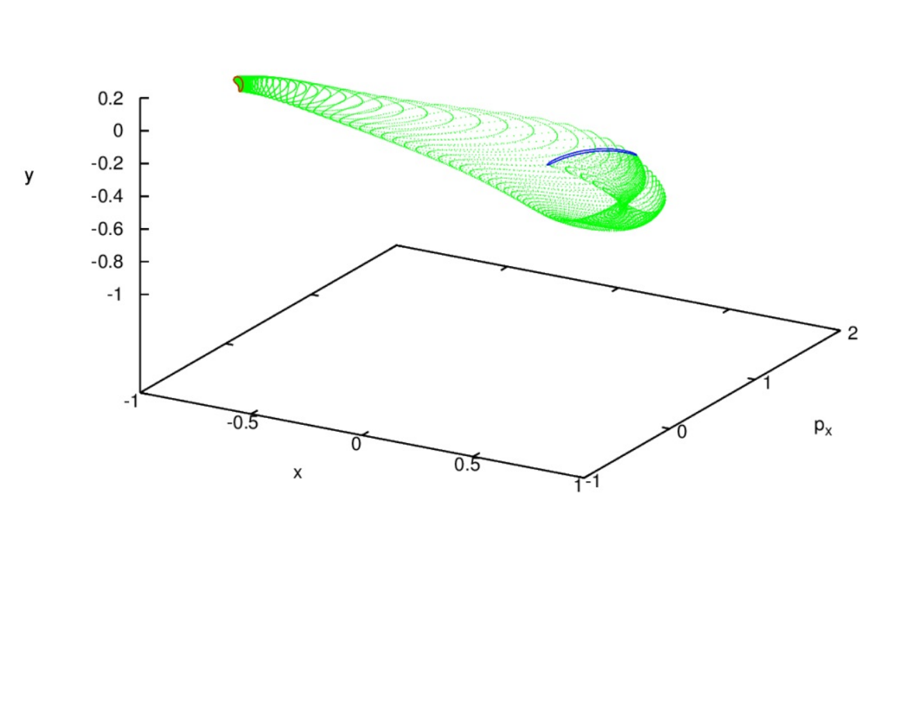
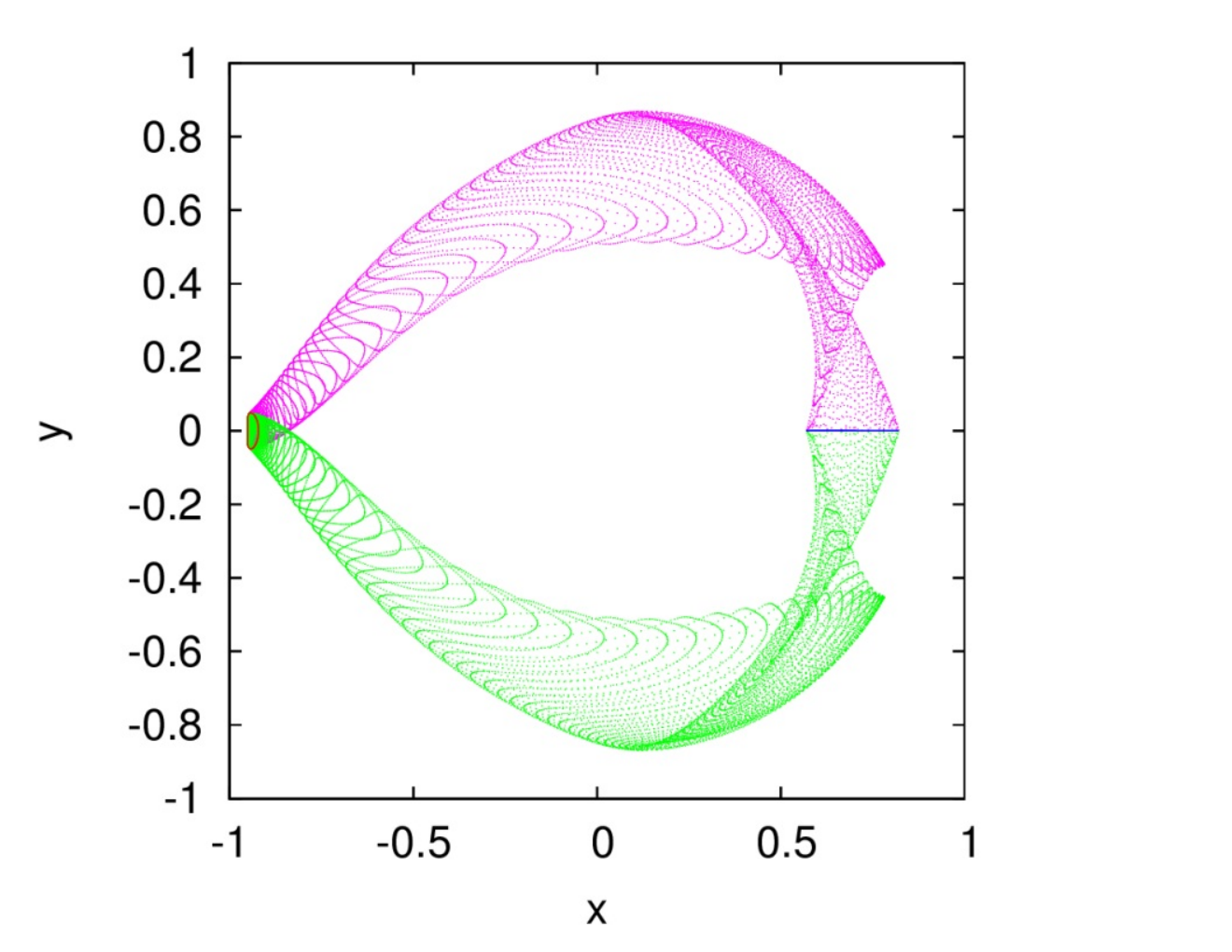
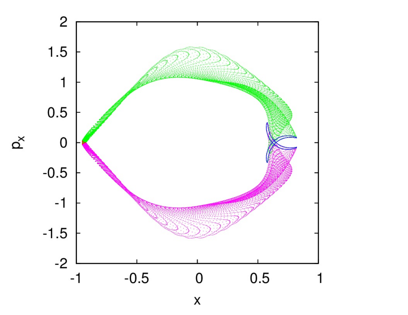
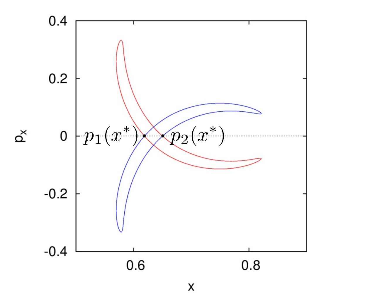
Numerical evidence suggests that intersection of $W^{u}\left(L(x^{\ast})\right)$ and $W^{s}\left(L(x^{\ast})\right)$ contains four homoclinic orbits. These orbits pass through four points, which can be seen on Figure 4 (right), and Figure 5. The intersections of $W^{u}\left(L(x^{\ast})\right)$ and $W^{s}\left(L(x^{\ast})\right)$ with $\{y=0\}$ are the “banana-shaped” loops, which intersect along the four points. Two of these, on the $x$ -axis, are the points from which start the $\mathbb{S}$ -symmetric homoclinic orbits. The remaining two homoclinic orbits are not $\mathbb{S}$ -symmetric. Let us use the notation $p_{1}(x^{\ast})$ for the left and $p_{2}\left(x^{\ast}\right)$ for the right one of the two $\mathbb{S}$ -symmetric intersection points.

Since the points $p_{1}\left(x^{\ast}\right),p_{2}\left(x^{\ast}\right)$ lie on $W^{u}\left(L(x^{\ast})\right),$ for any $x^{\ast}\in\mathbf{I}$ there exist two numbers $\omega_{1}(x^{\ast})$ , $\omega_{2}(x^{\ast})$ such that $p_{i}(x^{\ast})\in W^{u}\left(k_{0}(x^{\ast},\omega_{i}(x^{\ast}))\right)$ . For any $\theta\in\mathbb{R}$ ,

\begin{array}[]{l}\Phi_{\left(\theta-\omega_{i}(x^{\ast})\right)T(x^{\ast})/2\pi}\left(p_{i}(x^{\ast})\right)\\ \in W^{u}\left(\Phi_{\left(\theta-\omega_{i}(x^{\ast})\right)T(x^{\ast})/2\pi}(k_{0}(x^{\ast},\omega_{i}(x^{\ast})))\right)\\ =W^{u}\left(\Phi_{\left(\theta-\omega_{i}(x^{\ast})\right)T(x^{\ast})/2\pi}\Phi_{\omega_{i}(x^{\ast})T(x^{\ast})/2\pi}(q(x^{\ast}))\right)\\ =W^{u}\left(k_{0}(x^{\ast},\theta)\right).\end{array}

(26)

Since $\Phi_{t}(p_{i}(x^{\ast}))$ are $\mathbb{S}$ -symmetric, $p_{i}(x^{\ast})\in W^{s}\left(k_{0}(x^{\ast},-\omega_{i}(x^{\ast}))\right)$ . This implies

\begin{array}[]{l}\Phi_{\left(\theta-\omega_{i}(x^{\ast})\right)T(x^{\ast})/2\pi}\left(p_{i}(x^{\ast})\right)\\ \in W^{s}\left(\Phi_{\left(\theta-\omega_{i}(x^{\ast})\right)T(x^{\ast})/2\pi}\left(k_{0}(x^{\ast},-\omega_{i}(x^{\ast}))\right)\right)\\ =W^{s}\left(\Phi_{\left(\theta-\omega_{i}(x^{\ast})\right)T(x^{\ast})/2\pi}\Phi_{-\omega_{i}(x^{\ast})T(x^{\ast})/2\pi}(q(x^{\ast}))\right)\\ =W^{s}\left(k_{0}(x^{\ast},-2\omega_{i}(x^{\ast}))\right).\end{array}

(27)

We now define four homoclinic channels $\Gamma^{i,j}$ for $i,j=1,2$ as

	$\displaystyle\Gamma^{i,1}$	$\displaystyle=$	$\displaystyle\{\Phi_{\left(\theta-\omega_{i}(x^{\ast})\right)T(x^{\ast})/2\pi}(p_{i}(x^{\ast}))\|x^{\ast}\in\mathbf{I},\theta\in(-2\pi+\frac{\pi}{8},\frac{\pi}{8})\}$		(28)
	$\displaystyle\Gamma^{i,2}$	$\displaystyle=$	$\displaystyle\left\{\Phi_{\left(\theta-\omega_{i}(x^{\ast})\right)T(x^{\ast})/2\pi}(p_{i}(x^{\ast}))\|x^{\ast}\in\mathbf{I},\theta\in(0,2\pi)\right\}$

(These are depicted in Figure 9.) In total, we consider angles for the range $\theta\in\left[-2\pi,2\pi\right]$ , and for each $\theta$ we have two homoclinic channels. Numerical evidence suggests that $\Gamma^{i,j}$ lead to four well defined scattering maps

s_{0}^{i,j}:\mathcal{N}\rightarrow\mathcal{N}.

In fact, we can use any small fragment from the homoclinic orbits as a homoclinic channel, hence there are infinitely many of such channels. For our purposes though, restricting to four channels will turn out to be enough to apply Theorem 10.

We shall now show that $s_{0}^{i,j}$ are of the form (10). From (26), (27) we see that

$\displaystyle\Omega_{-}^{\Gamma^{i,j}}\left(\Phi_{\left(\theta-\omega_{i}(x^{\ast})\right)T(x^{\ast})/2\pi}\left(p_{i}(x^{\ast})\right)\right)$	$\displaystyle=k_{0}\left(x^{\ast},\theta\right),$	(29)
$\displaystyle\Omega_{+}^{\Gamma^{i,j}}\left(\Phi_{\left(\theta-\omega_{i}(x^{\ast})\right)T(x^{\ast})/2\pi}\left(p_{i}(x^{\ast})\right)\right)$	$\displaystyle=k_{0}\left(x^{\ast},\theta-2\omega_{i}(x^{\ast})\right),$	(30)
$\displaystyle\sigma^{\Gamma^{i,j}}\left(k_{0}\left(x^{\ast},\theta\right)\right)$	$\displaystyle=k_{0}\left(x^{\ast},\theta-2\omega_{i}(x^{\ast})\right),$	(31)

hence

s_{0}^{i,j}\left(x^{\ast},\theta\right)=k_{0}^{-1}\circ\sigma^{\Gamma^{i}}\circ k_{0}\left(x^{\ast},\theta\right)=\left(x^{\ast},\theta-2\omega_{i}(x^{\ast})\right).

(32)

4.3 Planar elliptic restricted three body problem

The planar restricted elliptic three body problem (PRE3BP) differs from the PRC3BP by the fact that the two larger bodies move on elliptic orbits of eccentricities $\varepsilon$ instead of circular orbits. The period of these orbits is $2\pi.$

After introducing the rotating coordinates (15), the Hamiltonian of PRE3BP can be rewritten as

H_{\varepsilon}(\mathbf{x},t)=H(\mathbf{x})+\varepsilon G(\mathbf{x},t)+O(\varepsilon^{2}),

(33)

where $H$ is the Hamiltonian of the PRC3BP (16), $G$ is $2\pi$ periodic over $t$ and is given by the formula [11]

G=\frac{1-\mu}{\left(r_{1}\right)^{3}}g(\mu,x,y,t)+\frac{\mu}{\left(r_{2}\right)^{3}}g(\mu-1,x,y,t),

(34)

g(\alpha,x,y,t)=\alpha(-2y\sin{t}+x\cos{t})-\alpha^{2}\cos{t}.

(35)

We note that in coordinates (15) the two primaries are no longer stationary. The larger primary rotates on a small elliptic orbit around the point $(x,y)=(\mu,0)$ . Similarly, the smaller primary rotates on an elliptic orbit around $(x,y)=(-1+\mu,0)$ . Note also that $r_{1}$ and $r_{2}$ do not measure the distance of the infinitesimal body to the primaries, but to the points $(\mu,0)$ and $(-1+\mu,0)$ , respectively.

We also note that this is a different coordinate system than the one used by Szebehely in [39], where he uses pulsating coordinates which places the larger bodies in fixed locations.

The movement of an infinitesimal body under the gravitational pull of the two primaries is given by the non-autonomous equation

\mathbf{\dot{x}}=J\nabla_{\mathbf{x}}H_{\varepsilon}(\mathbf{x},t).

(36)

Let $\Sigma_{t=\tau}=\left\{\left(\mathbf{x},t\right)|t=\tau\right\}$ and $\Phi_{\varepsilon,\tau,2\pi}:\Sigma_{t=\tau}\rightarrow\Sigma_{t=\tau}$ be the map induced by the time $2\pi$ shift along the flow of $H_{\varepsilon}$ . As mentioned in the previous section, numerical evidence suggests that, for $\varepsilon=0$ , the period $T(x^{\ast})$ of a Lyapunov orbit $L(x^{\ast})$ , satisfies

\frac{d}{dx^{\ast}}T(x^{\ast})\neq 0,

(37)

which by (32) is equivalent to $\Phi_{\varepsilon=0,\tau,2\pi}$ being a twist map on $\Lambda$ . We therefore formulate the following theorem.

We consider the system (33) in the phase space $\mathbb{R}^{4}\times\mathbb{T}^{1}$ , extended to include the time. The energy manifolds in the extended space are of the form $\tilde{M}(h)=M(h)\times\mathbb{T}^{1}$ , and the vector field is of the form $\tilde{X}=(X,1)$ , where $X$ is the Hamiltonian vector field associated to $H$ on $\mathbb{R}^{4}$ . The manifold $\tilde{\Lambda}=\Lambda\times\mathbb{T}^{1}$ is a normally hyperbolic invariant manifold with boundary for the flow $\tilde{\Phi}_{t}$ of $\tilde{X}$ in the extended phase space. (That is the flow associated to the PCR3BP, for $\varepsilon=0$ .)

Theorem 13.

Assume

\frac{d}{dx^{\ast}}T(x^{\ast})\neq 0

and also

\frac{d}{dx^{\ast}}H(q(x^{\ast}))\neq 0\qquad\mathchoice{\hbox{{for }}}{\hbox{{\firstchoice@false for }}}{\hbox{{\firstchoice@false for }}}{\hbox{{\firstchoice@false for }}}x^{\ast}\in\mathbf{I}.

(38)

Then for sufficiently small perturbation $\varepsilon$ the manifold $\tilde{\Lambda}$ is perturbed into a $O(\varepsilon)$ close normally hyperbolic manifold $\tilde{\Lambda}_{\varepsilon}$ , with boundary, which is invariant under the flow induced by (36). Moreover, there exists a Cantor set $\mathfrak{C}_{\varepsilon}$ of invariant tori in $\tilde{\Lambda}_{\varepsilon}$ .

Proof.

The proof is based on combining the persistence result for normally hyperbolic invariant manifolds theorem (Theorem 2), with the KAM Theorem 8. The technical issue that we need to address in this proof is the fact that $\tilde{\Lambda}$ is a normally hyperbolic manifold with boundary, but statement of Theorem 2 is for compact manifolds without boundary. To apply Theorem 2 we will modify the vector field induced by $H_{\varepsilon}$ , so that $\tilde{\Lambda}$ will become a compact manifold without boundary after the modification.

We now discuss the modification. Consider two closed intervals $\mathbf{I}^{\prime\prime},\mathbf{I}^{\prime}\subset\mathbb{R}$ satisfying $\mathbf{I}^{\prime\prime}\subset\mathrm{int}\mathbf{I}^{\prime},$ $\mathbf{I}^{\prime}\subset\mathrm{int}\mathbf{I}$ and let

$\displaystyle[a,b]$	$\displaystyle:$	$\displaystyle=\{H(L\left(x^{\ast}\right)):x^{\ast}\in\mathbf{I}\},$
$\displaystyle[a^{\prime},b^{\prime}]$	$\displaystyle:$	$\displaystyle=\{H(L\left(x^{\ast}\right)):x^{\ast}\in\mathbf{I}^{\prime}\},$
$\displaystyle[a^{\prime\prime},b^{\prime\prime}]$	$\displaystyle:$	$\displaystyle=\{H(L\left(x^{\ast}\right)):x^{\ast}\in\mathbf{I}^{\prime\prime}\}.$

We have $[a^{\prime\prime},b^{\prime\prime}]\subset(a^{\prime},b^{\prime}),$ $[a^{\prime},b^{\prime}]\subset(a,b)$ . Consider the following modified Hamiltonian

\widehat{H}_{\varepsilon}(\mathbf{x},t)=H\left(\mathbf{x}\right)+b\left(H(\mathbf{x})\right)\left[H_{\varepsilon}(\mathbf{x},t)-H\left(\mathbf{x}\right)\right],

(39)

where $b:\mathbb{R}\rightarrow[0,1]$ is a smooth ‘bump’ function, satisfying $b|_{\left[a^{\prime\prime},b^{\prime\prime}\right]}=1,$ $b|_{\mathbb{R}\setminus\left(a^{\prime},b^{\prime}\right)}=0$ .

Figure 6: Schematic plot of the modified Hamiltonian dynamics (left), and the gluing (right).

We now note some facts about $\widehat{H}_{\varepsilon}$ . For all points $\mathbf{x}$ with energies $H(\mathbf{x})$ outside of $\left(a^{\prime},b^{\prime}\right)$ , $\widehat{H}_{\varepsilon}(\mathbf{x},t)=H\left(\mathbf{x}\right)$ . This means that if we start with energies outside of $\left(a^{\prime},b^{\prime}\right)$ , we are dealing with the PCR3BP (see Figure 6), where energy is preserved. This in particular implies that if we start with a point with energy in $\left(a^{\prime},b^{\prime}\right)$ , then the energy along the solution of the flow for $\widehat{H}_{\varepsilon}$ will never leave $\left(a^{\prime},b^{\prime}\right)$ . (If it were to reach the boundary of $\left(a^{\prime},b^{\prime}\right)$ , this would contradict the fact that on the boundary of $\left(a^{\prime},b^{\prime}\right)$ the Hamiltonian is autonomous and the energy is preserved). Another important fact is that for energies inside of $\left[a^{\prime\prime},b^{\prime\prime}\right]$ the flow of (39) coincides with the solution for PER3BP. For $\varepsilon=0$ , the manifold $\tilde{\Lambda}$ is invariant under the flow of $\widehat{H}_{\varepsilon}$ .

The manifold $\tilde{\Lambda}$ is diffeomorphic to a $3$ -dimensional annulus $\mathbf{I}\times\mathbb{T}^{2}$ , with one boundary component $L(a)\times\mathbb{T}^{1}$ and the other boundary component $L(b)\times\mathbb{T}^{1}$ , where $L(a)$ , $L(b)$ are the Lyapunov orbits at energies $a$ , $b$ , respectively. We restrict to the energy level sets $\bigcup_{h\in[a,b]}\tilde{M}(h)$ , and glue another copy of $\bigcup_{h\in[a,b]}\tilde{M}(h)$ , such that the energy level of $b$ in the first copy matches with the energy level of $b$ in the second copy (see Figure 6). Note that for energies in $\left[a,b\right]\setminus\left[a^{\prime},b^{\prime}\right]$ , $\hat{H}_{0}$ is preserved along each level set. We can modify the vector field so that it is smooth along the gluing, that $L(a),L(b)$ remain invariant, and so that the annulus can also be smoothly glued along $L(a)$ . This modification is performed outside of $\bigcup_{h\in[a^{\prime},b^{\prime}]}M(h)$ . We denote this vector field by $\hat{X}_{\varepsilon}$ . Let $\widehat{M}$ be the manifold in the extended phase space obtained by the above gluing of level sets, that is $\widehat{M}=\bigcup_{h\in[a,b]}M(h)\sqcup\bigcup_{h\in[a,b]}M(h)$ . The two copies of $\tilde{\Lambda}$ are smoothly glued along $L(a)\times\mathbb{T}^{1}$ , and the corresponding gluing of the the two copies of $\tilde{\Lambda}$ inside $\widehat{M}$ results in a $3$ -dimensional annulus $\widehat{\Lambda}$ whose boundary components at both ends are identical to $L(a)\times\mathbb{T}^{1}$ . Hence, for $\varepsilon=0$ we have that $\widehat{\Lambda}$ is diffeomorphic to a $3$ -dimensional torus. Thus, $\widehat{\Lambda}$ can be viewed as a compact, normally hyperbolic invariant manifold for $\hat{X}_{0}$ .

For $\varepsilon>0$ sufficiently small, we apply Theorem 2, to a time shift map along the flow of $\hat{X}_{\varepsilon}$ , obtaining $\widehat{\Lambda}_{\varepsilon}$ .

Note that the flow corresponding to the vector field $\hat{X}_{\varepsilon}$ has no effect on the boundary $L(a),L(b)$ of the annulus $\tilde{\Lambda}$ . As $\widehat{\Lambda}$ consists of two copies of $\tilde{\Lambda}$ , we can now restrict to only one of the copies, concluding the existence of a normally hyperbolic manifold with boundary $\tilde{\Lambda}_{\varepsilon}\subset\widehat{\Lambda}_{\varepsilon}$ that survives to $\tilde{\Lambda}$ . The boundary of $\tilde{\Lambda}_{\varepsilon}$ is invariant under the flow of $\hat{X}_{\varepsilon}$ . The only role of $\widehat{\Lambda}$ was to be able to apply Theorem 2 ad litteram, as $\widehat{\Lambda}$ can be viewed as a compact manifold without boundary. From now we give up entirely on $\widehat{\Lambda}$ , and we refer only to $\tilde{\Lambda}_{\varepsilon}$ .

We remark here that $\tilde{\Lambda}_{\varepsilon}$ depends on the choice of the ‘bump’ function $b$ . We will address this issue in what follows.

For $\left(\mathbf{x},\tau\right)\in\tilde{\Lambda}$ and fixed $t>0$ , the eigenvalues of $D_{\mathbf{x}}\tilde{\Phi}_{t}(\mathbf{x},\tau)$ are $\lambda_{1},\lambda_{2},1,1,1,$ with $\left|\mathrm{re}\lambda_{1}\right|>1>\left|\mathrm{re}\lambda_{2}\right|$ . We can therefore choose $\mu$ from Definition 1 arbitrarily close to one, which by Theorem 2 means that $\widehat{\Lambda}_{\varepsilon}$ are $C^{l-1}$ smooth with arbitrarily large $l$ (for us it is enough to have $l\geq 7$ ).

Let $\Lambda_{\varepsilon,\tau}=\tilde{\Lambda}_{\varepsilon}\cap\Sigma_{t=\tau}$ . Let $\hat{\Phi}_{\varepsilon,\tau,t}$ be the solution of the ODE induced by (39). Since $\widehat{H}_{\varepsilon}$ is $2\pi$ periodic, we can consider the map $\hat{\Phi}_{\varepsilon,\tau,2\pi}:\Lambda_{\varepsilon,\tau}\rightarrow\Lambda_{\varepsilon,\tau}$ . Our next step is to apply Theorem 8 to it. It is a well known property of Hamiltonian systems that a time shift map along a trajectory of the system is exact symplectic, hence $\hat{\Phi}_{\varepsilon,\tau,2\pi}$ is exact symplectic with the standard symplectic form. By Lemma 3, $\omega|_{\Lambda}$ is non-degenerate. Let us now consider the reference manifold $\mathcal{N}$ given by (22), and the parameterization $k_{0}$ from (23). By Theorem 6, it is possible to choose coordinates $k_{\varepsilon,\tau}:\mathcal{N}\rightarrow\Lambda_{\varepsilon,\tau}$ so that $k_{\varepsilon,\tau}^{\ast}\omega|_{\Lambda_{\varepsilon,\tau}}=k_{0}^{\ast}\omega|_{\Lambda}=\omega_{\mathcal{N}}$ . We can now define a $C^{l-1}$ smooth family of exact symplectic maps

r_{\varepsilon,\tau,2\pi}:\mathcal{N}\rightarrow\mathcal{N}

r_{\varepsilon,\tau,2\pi}=k_{\varepsilon,\tau}^{-1}\circ\hat{\Phi}_{\varepsilon,\tau,2\pi}\circ k_{\varepsilon,\tau}.

By (24) and (37) we see that $r_{0,\tau,2\pi}=r_{0,2\pi}$ is a twist map. We can therefore apply Theorem 8 to obtain a family of invariant tori for $r_{\varepsilon,\tau,2\pi}$ . The Lyapunov orbits on $\Lambda$ play the role of the unperturbed tori of Theorem 8. Their rotation numbers are determined by the choice of $x^{\ast}\in\mathbf{I}.$ We thus have a family of invariant tori $u_{x^{\ast}}$ of $r_{\varepsilon,\tau,2\pi}$ for a Cantor set $\mathfrak{G}_{\varepsilon,\tau}^{\mathbf{I}}$ of $x^{\ast}$ in $\mathbf{I}.$ We have now obtained our Cantor set $\mathfrak{C}_{\varepsilon}$ defined by

\mathfrak{C}_{\varepsilon}=\left\{\left(k_{\varepsilon,\tau}\left(u_{x^{\ast}}\right),\tau\right):x^{\ast}\in\mathfrak{G}_{\varepsilon,\tau}^{\mathbf{I}}\subset\mathbf{I},\tau\in\mathbb{T}^{1}\right\},

as claimed in the statement of the theorem. What is left though, is to deal with the fact that these tori were obtained for the modified Hamiltonian.

Let $\mathbf{I}^{\prime\prime\prime}\subset\mathrm{int}\mathbf{I}^{\prime\prime}$ and $\left[a^{\prime\prime\prime},b^{\prime\prime\prime}\right]=\{H(L\left(x^{\ast}\right)):x^{\ast}\in\mathbf{I}^{\prime\prime\prime}\}$ . By the smooth dependence of the flow on the parameter $\varepsilon$ , for sufficiently small $\varepsilon_{0}$ , for any $\mathbf{x}\in\Lambda_{\varepsilon,\tau}$ satisfying $H\left(\mathbf{x}\right)\in\left[a^{\prime\prime\prime},b^{\prime\prime\prime}\right]$ , any $t\in\left[0,2\pi\right]$ and any $\varepsilon\in\left[0,\varepsilon_{0}\right]$ , we have $H(\hat{\Phi}_{\varepsilon,\tau,t}\left(\mathbf{x}\right))\in\left[a^{\prime\prime},b^{\prime\prime}\right]$ . Since for energies from $\left[a^{\prime\prime},b^{\prime\prime}\right]$ the trajectory for (39) coinsides with the trajectroy for the PER3BP, we have that $\hat{\Phi}_{\varepsilon,\tau,t}\left(\mathbf{x}\right)=\Phi_{\varepsilon,\tau,2\pi}\left(\mathbf{x}\right)$ , so, the established invariant tori from $\mathfrak{C}_{\varepsilon,\tau}^{\mathbf{I}^{\prime\prime\prime}}$ are in fact true invariant tori for the PER3BP. We can restrict $\mathfrak{C}_{\varepsilon}$ to these tori, which finishes our proof. ∎

Remark 14.

The invariant tori in $\mathfrak{C}_{\varepsilon}$ separate $\tilde{\Lambda}_{\varepsilon}$ forming an obstruction, which prohibits a large change of energy using only the inner dynamics on $\tilde{\Lambda}_{\varepsilon}$ .

Remark 15.

For existence of diffusion we need Theorem 13 only for the persistence of the manifold $\tilde{\Lambda}$ under perturbation. Since $\tilde{\Lambda}$ is a manifold with a boundary, the KAM part of the proof of Theorem 13 allows us to obtain persistence of the boundaries of the manifold under perturbation.

We now turn to the computation of perturbed scattering maps.

Lemma 16.

For any $x^{\ast}\in\mathbf{I}$ and $i,j=1,2$

s_{\varepsilon,\tau}^{i,j}=s_{0}^{i,j}+\varepsilon J\nabla S_{0,\tau}^{i,j}\circ s_{0}^{i,j}+O\left(\varepsilon^{2}\right),

(40)

and

	$\displaystyle\frac{\partial S_{0,\tau}^{i,j}}{\partial\theta}(s_{0}^{i,j}\left(x^{\ast},\theta\right))$	$\displaystyle=\frac{T(x^{\ast})}{2\pi}[-G\left(\Phi_{\theta T(x^{\ast})/2\pi}\left(q(x^{\ast})\right),\tau\right)$
		$\displaystyle\qquad\quad+G\left(\Phi_{\left(\theta-2\omega_{i}(x^{\ast})\right)T(x^{\ast})/2\pi}\left(q(x^{\ast})\right),\tau\right)$
		$\displaystyle\quad-\int_{-\infty}^{0}\frac{\partial G}{\partial t}\left(\Phi_{u+(\theta-\omega_{i}(x^{\ast}))T(x^{\ast})/2\pi}\left(p_{i}(x^{\ast})\right),\tau+u\right)$
		$\displaystyle\qquad\quad-\frac{\partial G}{\partial t}\left(\Phi_{u+\theta T(x^{\ast})/2\pi}\left(q(x^{\ast})\right),\tau+u\right)du$
		$\displaystyle\quad-\int_{0}^{\infty}\frac{\partial G}{\partial t}\left(\Phi_{u+\left(\theta-\omega_{i}(x^{\ast})\right)T(x^{\ast})/2\pi}\left(p_{i}(x^{\ast})\right),\tau+u\right)$
		$\displaystyle\qquad\quad-\frac{\partial G}{\partial t}\left(\Phi_{u+\left(\theta-2\omega_{i}(x^{\ast})\right)T(x^{\ast})/2\pi}\left(q(x^{\ast})\right),\tau+u\right)du].$

Proof.

The proof follows by substituting (29–32) into (8–9) and computing the partial derivative with respect to $\theta$ . We give the details in A. ∎

We are now ready to formulate a theorem that can be used to obtain a proof of diffusion in the restricted three body problem.

Theorem 17.

Assume that for a given interval $\mathbf{I}$ , for any $x^{\ast}\in\mathbf{I}$ the manifolds $W^{u}\left(L(x^{\ast})\right),$ $W^{s}\left(L(x^{\ast})\right)$ intersect transversally, and that we have two points $p_{1}(x^{\ast})\neq p_{2}(x^{\ast})$

p_{1}(x^{\ast}),p_{2}(x^{\ast})\in W^{u}\left(L(x^{\ast})\right)\cap W^{s}\left(L(x^{\ast})\right)\cap\{y=0,p_{x}=0\}.

Assume that for $i,j=1,2$ the $\Gamma^{i,j}$ defined in (28) are homoclinic channels. Assume also that there exists $\tau^{\ast}\in(0,2\pi]$ such that for any $x^{\ast}\in\mathbf{I}$ and for any $\theta\in\mathbb{T}^{1}$ there exist $i_{1},i_{2},j_{1},j_{2}\in\{1,2\},$ such that

	$\displaystyle\frac{\partial S_{0,\tau^{\ast}}^{i_{1},j_{1}}}{\partial\theta}(s_{0}^{i_{1},j_{1}}\left(x^{\ast},\theta\right))$	$\displaystyle>0,$			(41)
	$\displaystyle\frac{\partial S_{0,\tau^{*}}^{i_{2},j_{2}}}{\partial\theta}(s_{0}^{i_{2},j_{2}}\left(x^{\ast},\theta\right))$	$\displaystyle<0.$			(42)

Also assume that the assumptions of Theorem 13 hold. Then there exists an $\varepsilon^{\ast}>0$ such that for all $\varepsilon\in(0,\varepsilon^{\ast})$ , any $I_{1},I_{2}\in\mathbf{I}$ , $I_{1}<I_{2}$ and any $\rho>0$ there exist heteroclinic orbits from $B_{\rho}^{<}(I_{1})$ to $B_{\rho}^{>}(I_{2})$ and a heteroclinic orbit from $B_{\rho}^{>}(I_{2})$ to $B_{\rho}^{<}(I_{1})$ .

Proof.

By Theorem 13 the manifold persists under perturbation.

By (41) the assumption (12) from Theorem 10 holds, hence there exists a homoclinic orbit from $B_{\rho}^{<}(I_{1})$ to $B_{\rho}^{>}(I_{2})$ .

The proof of a homoclinic orbit from $B_{\rho}^{>}(I_{2})$ to $B_{\rho}^{<}(I_{1})$ also follows from Theorem 10, using (42). ∎

Remark 18.

For any $I_{1}<I_{2},$ taking sufficiently small $\rho$ ensures that the set $B_{\rho}^{>}(I_{2})$ has higher energy than $B_{\rho}^{<}(I_{1})$ . Thus the homoclinic orbits from Theorem 17 involve a change of energy for arbitrarily small $\varepsilon>0.$ The size of the change of the energy is determined by the choice of $I_{1},I_{2}$ and does not depend on $\varepsilon$ .

Remark 19.

Note that Theorem 17 establishes existence of diffusion by showing that if there is no inner diffusion, there is diffusion along homoclinic excursions. So, in either case there is diffusion. The KAM theorem shows that there is no inner diffusion hence it is the alternative of homoclinic excursions that happens.

5 Numerical verification of the hypothesis of Theorem 17

We shall give numerical evidence that assumptions (41–42) from Theorem 17 are satisfied. For this we need to numerically compute integrals along the orbits $\Phi_{t}\left(p_{1}(x^{\ast})\right)$ , $\Phi_{t}\left(p_{2}(x^{\ast})\right)$ and $\Phi_{t}\left(q(x^{\ast})\right).$ We describe the procedure of how this can be done.

The $q(x^{\ast})$ and $T(x^{\ast})$ are found as follows. We consider a section $\Sigma=\left\{y=0\right\}$ and a Poincaré map $P:\Sigma\rightarrow\Sigma$ . If for a point $q=(x,0,0,p_{y})\in\Sigma$ we have $\pi_{p_{x}}P(q)=0$ , then by the symmetry property (19), the point $q$ lies on a periodic orbit (the Poincaré map $P$ makes a half turn along the orbit starting from $q$ ). Thus, for a given $x^{\ast}$ , the point $q(x^{\ast})=(x,0,0,\kappa(x^{\ast}))$ can be found by considering a function $h:\mathbb{R\rightarrow R}$ defined as $h(p_{y})=\pi_{p_{x}}P(x^{\ast},0,0,p_{y}),$ and numerically solving $h(p_{y})=0$ . Having found $q(x^{\ast}),$ the first time to reach $\Sigma$ along the flow is $T(x^{\ast})/2.$

We now discuss how we compute $p_{1}(x^{\ast})$ and $p_{2}(x^{\ast}).$ The $q(x^{\ast})$ is a fixed point for the $T(x^{\ast})$ time shift along the trajectory map $\Phi_{T(x^{\ast})}$ . The one dimensional unstable manifold of the map $\Phi_{T(x^{\ast})}$ at $q(x^{\ast})$ is equal to the unstable fiber $W^{u}(q(x^{\ast}))$ of the flow. We consider the matrix $A=D\Phi_{T(x^{\ast})}(q(x^{\ast})).$ The unstable eigenvector $v$ of $A$ is colinear with $T_{q(x^{\ast})}W^{u}(q(x^{\ast})).$ For sufficiently small $h\in\mathbb{R}$ , the point $q_{h}=q(x^{\ast})+hv$ is a good approximation of a point on $W^{u}(q(x^{\ast})),$ and $v$ is a good approximation of $T_{q_{h}}W^{u}(q(x^{\ast}))$ . We can propagate $q_{h}$ along the flow to the section $\Sigma_{x>0}=\{y=0,x>0\}$ . Let $\tau(h)$ be the time from $q_{h}$ to $\Sigma_{x>0}$ . If we can find such $h$ , so that $\pi_{p_{x}}\Phi_{\tau(h)}(q_{h})=0$ , then by the symmetry property (19), the point $\Phi_{\tau(h)}(q_{h})$ is an approximation of a point on a symmetric homoclinic orbit to $L(x^{\ast})$ . This way we numerically compute $p_{i}(x^{\ast})$ as $\Phi_{\tau(h_{i})}(q_{h_{i}})$ , for $i=1,2$ . From the computation we also obtain $\omega_{i}(x^{\ast})=2\pi\tau(h_{i})/T(x^{\ast})$ mod $2\pi$ , for $i=1,2$ .

For any $q\in L(x^{\ast}),$ the unstable fiber $W^{u}(q)$ can be computed by propagating $W^{u}(q(x^{\ast}))$ along the flow. Thus, since $p_{i}(x^{\ast})_{-}\in L(x^{\ast})$ , the $T_{p_{i}(x^{\ast})}W^{u}(p_{i}(x^{\ast})_{-})$ are approximated by $D\Phi_{\tau(h_{i})}(q_{h_{i}})v$ , for $i=1,2$ .

We now focus on $x^{\ast}=-0.95$ . Using the above outlined procedure, we obtain the following numerical results:

$\displaystyle q(x^{\ast})$	$\displaystyle=$	$\displaystyle\left(-0.95,0,0,-0.8413472441\right),$
$\displaystyle T(x^{\ast})$	$\displaystyle=$	$\displaystyle 3.041751775,$
$\displaystyle p_{1}(x^{\ast})$	$\displaystyle=$	$\displaystyle\left(0.6207553555,0,0,1.38203433\right),$
$\displaystyle p_{2}(x^{\ast})$	$\displaystyle=$	$\displaystyle\left(0.6514581118,0,0,1.334413389\right),$
$\displaystyle\omega_{1}(x^{\ast})$	$\displaystyle=$	$\displaystyle 1.451540621,$
$\displaystyle\omega_{2}(x^{\ast})$	$\displaystyle=$	$\displaystyle-0.2527863329,$

and $T_{p_{i}(x^{\ast})}W^{u}(p_{i}(x^{\ast})_{-})=\mathrm{span}\left\{v_{i}\right\}$ , for $i=1,2$ , with

\begin{array}[]{rrrr}v_{1}~=~(1,&-9.823658901,&17.9416819,&-1.60121149),\\ v_{2}~=~(1,&-4.42688411,&8.405095683,&-1.503579624).\end{array}

(43)

We use a linearization to approximate $W^{u}(q).$ Close to $L(x^{\ast})$ , such approximation is accurate. We integrate the flow using a high precision (order 20) Taylor method. Thus, the resulting approximation of the points $p_{1}(x^{\ast}),$ $p_{2}(x^{\ast})$ is reliable.

Based on the above $p_{1}(x^{\ast}),$ $p_{2}(x^{\ast}),$ we can numerically compute the homoclinic orbits $\Phi_{t}\left(p_{1}(x^{\ast})\right)$ , $\Phi_{t}\left(p_{2}(x^{\ast})\right)$ (see Figure 7), together with the corresponding fragments of the homoclinic channels $\Gamma^{i,j}$ defined in (28), for $i,j=1,2$ .

Figure 7: Homoclinic orbit

\Phi_{t}(p_{1}(x^{\ast}))

(top) and

\Phi_{t}(p_{2}(x^{\ast}))

(bottom) in black, and their fragments on

\Gamma^{i,j}

, in green and red, for

x^{\ast}=-0.95.

Figure 8: The plots of

\theta\rightarrow\frac{\partial S_{0,\tau^{\ast}}^{i,j}}{\partial\theta}(s_{0}^{i,j}(x^{\ast},\theta)),

for

\tau^{\ast}=0

and

x^{\ast}=-0.95.

The corresponding indexes

i,j

are indicated on the plot.

The $\Gamma^{i,j}$ are indeed homoclinic channels, i.e. satisfy conditions (i) and (ii) from Definition 4. We describe how this has been investigated. Condition (i) follows from the fact that $W^{s}\left(\Lambda\right)$ and $W^{u}\left(\Lambda\right)$ intersect transversally. To show (ii) we shall first fix an $i\in\{1,2\}$ and consider $\mathbf{x}=p_{i}(x^{\ast})\in\Gamma^{i,1}\cup\Gamma^{i,2}.$ We need to verify that

T_{\mathbf{x}}\Gamma^{i}\oplus T_{\mathbf{x}}W^{u}\left(\mathbf{x}_{-}\right)=T_{\mathbf{x}}W^{u}\left(\Lambda\right).

(44)

We shall use the fact that

T_{\mathbf{x}}\Gamma^{i}=\mathrm{span}\left(\frac{d}{dx^{\ast}}p_{i}(x^{\ast}),F(p_{i}(x^{\ast}))\right).

Focusing on $x^{\ast}=-0.95,$ the numerical results are:

\begin{array}[]{rrrr}\mathrm{span}\left\{\frac{d}{dx^{\ast}}p_{1}(x^{\ast})\right\}=\,\mathrm{span}\{(1,&0,&0,&-1.826312946)\},\\ \mathrm{span}\left\{F(p_{1}(x^{\ast}))\right\}=\,\mathrm{span}\{(0,&1,&-1.60121149,&0)\},\end{array}

(45)

and

\begin{array}[]{rrrr}\mathrm{span}\left\{\frac{d}{dx^{\ast}}p_{2}(x^{\ast})\right\}=\,\mathrm{span}\{(1,&0,&0,&-1.898743306)\},\\ \mathrm{span}\left\{F(p_{2}(x^{\ast}))\right\}=\,\mathrm{span}\{(0,&1,&-1.503579624,&0)\}.\end{array}

(46)

Comparing (45) with (43), it can easily be checked that $v_{1},$ $\frac{d}{dx^{\ast}}p_{1}(x^{\ast}),$ $F(p_{1}(x^{\ast}))$ are linearly independent. From (46) and (43) we also see that so are $v_{2},$ $\frac{d}{dx^{\ast}}p_{2}(x^{\ast}),$ $F(p_{2}(x^{\ast}))$ . This implies (44). Transversality is preserved along the flow, which demonstrates that (ii) holds for the unstable manifold. For the stable manifold, (ii) follows from the symmetry of the PCR3BP.

We now move to the computation of $\frac{\partial S_{0,\tau^{\ast}}^{i,j}}{\partial\theta}$ . We take $\tau^{\ast}=0.$ Employing Lemma 16, we can numerically compute and plot the functions

\theta\rightarrow\frac{\partial S_{0,\tau^{\ast}}^{i,j}}{\partial\theta}(s_{0}^{i,j}(x^{\ast},\theta)),

for $i,j=1,2$ . The plots are given in Figure 8.

Figure 9: Homoclinic orbit

\Phi_{t}(p_{1}(x^{\ast}))

(top) and

\Phi_{t}(p_{2}(x^{\ast}))

(bottom) in black, together with the homoclinic channels

\Gamma^{i,j}

, in green and red, for

x^{\ast}\in\mathbf{I}=\left(-0.955,-0.945\right)

Figure 10: The plots of

\theta\rightarrow\frac{\partial S_{0,\tau^{\ast}}^{i,j}}{\partial\theta}(s_{0}^{i,j}(x^{\ast},\theta)),

for

\tau^{\ast}=0

and

x^{\ast}=-0.955,-0.9525,-0.95,-0.9475,-0.945

. The corresponding indexes

i,j

are indicated on the plot.

We have focused on the particular value $x^{\ast}=-0.95$ only because it is a round number, and because for such $x^{\ast}$ the energy of the Lyapunov orbit $L(x^{\ast})$ is close to the energy of the comet Oterma. For different $x^{\ast}$ one observes similar plots. For instance, for any $x^{\ast}$ within a $5\cdot 10^{-3}$ distance of $-0.95$ one obtains plots with the same properties (see Figures 9 and 10). This means that we can choose

\mathbf{I}=\left(-0.955,-0.945\right).

In Figure 10 we see that for any point on $L(x^{\ast})$ for $x^{\ast}\in\mathbf{I}$ , by taking $\theta\leq\frac{\pi}{8}$ we can always choose a scattering map for which condition (41) is satisfied. Similarly, condition (42) is satisfied for $\theta\geq 0$ . For any point on $L(x^{\ast})$ we can therefore choose a scattering map satisfying (41) or (42). Thus, by Theorem 17, the computations give evidence of diffusion for any sufficiently small $\varepsilon$ .

In Figure 11 we see the plots of $x^{\ast}\rightarrow T(x^{\ast})$ and $x^{\ast}\rightarrow H(q(x^{\ast}))$ . Clearly the assumptions (37), (38), which are the assumptions of Theorem 13, are reflected to hold in the calculations.

Figure 11: The plots of

x^{\ast}\rightarrow T(x^{\ast})

(left) and

x^{\ast}\rightarrow H(q(x^{\ast}))

(right).

The Lyapunov orbits $L(x^{\ast})$ for $x^{\ast}\in\mathbf{I}$ are depicted in Figure 2. The width of the interval $\mathbf{I}$ , when translated to real distance in the Jupiter-Sun system, is roughly equivalent to over $7$ million kilometers. We therefore see that our mechanism leads to macroscopic diffusion distances. The homoclinic channels depicted in Figure 9 give us an idea of the paths along which diffusion takes place and of its scale.

6 Future work

In the forthcoming work we plan to validate the assumptions of Theorem 17. To do so the following ingredients need to be checked.

We need to check that the homoclinic channels are well defined. This means that we need to validate the conditions from Definition 4. These will follow from the fact that the stable and unstable manifolds of the family of the Lyapunov orbits intersect transversally. Such validation has already been performed in [7], hence we do not anticipate any difficulties associated with this step.

We need to verify conditions (37), (38), needed for the Theorem 13. Again, based on the results obtained in [7], we think that this verification should be straightforward, since it involves finite computation along Lyapunov orbits.

The last step requires the verification of conditions (41), (42) which are the key assumptions of Theorem 17. This last step will likely cause most difficulties. It involves a computation of integrals over reals. Over a finite time interval these can be validated using a rigorous computer assisted enclosure of the homoclinic orbits computed in [7]. What will remain is to obtain an estimate on the tails of the integrals, which will need to follow from analytic arguments. We believe that such validation is possible and plan to address the problem in the future.

We believe that our approach and the mechanism presented in this paper can be used to produce a computer assisted proof of diffusion in the restricted three body problem.

Acknowledgments

We would like to thank the two anonymous reviewers for their suggestions and comments, which helped us to improve the manuscript.

The research of M.J. Capiński was partially supported by the Polish National Science Center grant 2012/05/B/ST1/00355. The research of M. Gidea was partially supported by the NSF grant DMS-1515851. The research of R. de la Llave was partially supported by the NSF grant DMS-1500943.

Appendix A Proof of Lemma 16

Let us fix $x^{\ast}\in\mathbf{I}$ . In order to keep notations short, we write $q$ , $p_{1}$ , $p_{2}$ , $\omega_{1}$ , $\omega_{2},$ $T$ for $q(x^{\ast})$ , $p_{1}(x^{\ast})$ , $p_{2}(x^{\ast})$ , $\omega_{1}(x^{\ast})$ , $\omega_{2}(x^{\ast})$ , $T(x^{\ast})$ , respectively.

Equality (40) follows from (8). Substituting (29–31) into (9) we see that

	$\displaystyle S_{0,\tau}^{i,j}\left(x^{\ast},\theta\right)$	$\displaystyle=\int_{-\infty}^{0}G\left(\Phi_{u}\circ\Phi_{\left(\theta+\omega_{i}\right)T/2\pi}\left(p_{i}\right),\tau+u\right)$
		$\displaystyle\qquad\qquad\qquad-G\left(\Phi_{u}\circ k_{0}\left(x^{\ast},\theta+2\omega_{i}\right)\mathbf{,}\tau+u\right)du$
		$\displaystyle\quad+\int_{0}^{+\infty}G\left(\Phi_{u}\circ\Phi_{\left(\theta+\omega_{i}\right)T/2\pi}\left(p_{i}\right),\tau+u\right)$
		$\displaystyle\qquad\qquad\qquad-G\left(\Phi_{u}\circ k_{0}\left(x^{\ast},\theta\right)\mathbf{,}\tau+u\right)du$
		$\displaystyle=\int_{-\infty}^{\theta T/2\pi}G\left(\Phi_{u+\omega_{i}T/2\pi}\left(p_{i}\right),\tau+u-\theta T/2\pi\right)$
		$\displaystyle\qquad\qquad\qquad-G\left(\Phi_{u+2\omega_{i}T/2\pi}(q)\mathbf{,}\tau+u-\theta T/2\pi\right)du$
		$\displaystyle\quad+\int_{\theta T/2\pi}^{+\infty}G\left(\Phi_{u+\omega_{i}T/2\pi}\left(p_{i}\right),\tau+u-\theta T/2\pi\right)$
		$\displaystyle\qquad\qquad\qquad-G\left(\Phi_{u}\left(q\right),\tau+u-\theta T/2\pi\right)du.$

This gives

$\displaystyle\frac{\partial S_{0,\tau}^{i,j}}{\partial\theta}\left(x^{\ast},\theta\right)$	$\displaystyle=$	$\displaystyle\frac{T}{2\pi}[-G\left(\Phi_{\theta+2\omega_{i}T/2\pi}\left(q\right),\tau\right)+G\left(\Phi_{\theta}\left(q\right),\tau\right)$
		$\displaystyle-\int_{-\infty}^{\theta T/2\pi}\frac{\partial G}{\partial t}\left(\Phi_{u+\omega_{i}T/2\pi}\left(p_{i}\right),\tau+u-\theta T/2\pi\right)$
		$\displaystyle\qquad\qquad-\frac{\partial G}{\partial t}\left(\Phi_{u+2\omega_{i}}\left(q\right),\tau+u-\theta T/2\pi\right)du$
		$\displaystyle-\int_{\theta T/2\pi}^{\infty}\frac{\partial G}{\partial t}\left(\Phi_{u+\omega_{i}T/2\pi}\left(p_{i}\right),\tau+u-\theta T/2\pi\right)$
		$\displaystyle\qquad\qquad-\frac{\partial G}{\partial t}\left(\Phi_{u}\left(q\right),\tau+u-\theta T/2\pi\right)du],$

hence by (32),

	$\displaystyle\frac{\partial S_{0,\tau}^{i,j}}{\partial\theta}\left(s_{0}^{i,j}\left(x^{\ast},\theta\right)\right)$
	$\displaystyle=\frac{T}{2\pi}[-G\left(\Phi_{\theta}\left(q\right),\tau\right)+G\left(\Phi_{\theta-2\omega_{i}T/2\pi}\left(q\right),\tau\right)$
	$\displaystyle\quad-\int_{-\infty}^{\left(\theta-2\omega_{i}\right)T/2\pi}\frac{\partial G}{\partial t}\left(\Phi_{u+\omega_{i}T/2\pi}\left(p_{i}\right),\tau+u-\left(\theta-2\omega_{i}\right)T/2\pi\right)$
	$\displaystyle\qquad\qquad-\frac{\partial G}{\partial t}\left(\Phi_{u+2\omega_{i}T/2\pi}\left(q\right),\tau+u-\left(\theta-2\omega_{i}\right)T/2\pi\right)du$
	$\displaystyle\quad-\int_{\left(\theta-2\omega_{i}\right)T/2\pi}^{\infty}\frac{\partial G}{\partial t}\left(\Phi_{u+\omega_{i}T/2\pi}\left(p_{i}\right),\tau+u-\left(\theta-2\omega_{i}\right)T/2\pi\right)$
	$\displaystyle\qquad\qquad-\frac{\partial G}{\partial t}\left(\Phi_{u}\left(q\right),\tau+u-\left(\theta-2\omega_{i}\right)T/2\pi\right)du]$
	$\displaystyle=\frac{T}{2\pi}[-G\left(\Phi_{\theta}\left(q\right),\tau\right)+G\left(\Phi_{\theta-2\omega_{i}T/2\pi}\left(q\right),\tau\right)$
	$\displaystyle\quad-\int_{-\infty}^{0}\frac{\partial G}{\partial t}\left(\Phi_{u+\left(\theta-\omega_{i}\right)T/2\pi}\left(p_{i}\right),\tau+u\right)-\frac{\partial G}{\partial t}\left(\Phi_{u+\theta T/2\pi}\left(q\right),\tau+u\right)du$
	$\displaystyle\quad-\int_{0}^{\infty}\frac{\partial G}{\partial t}\left(\Phi_{u+\left(\theta-\omega_{i}\right)T/2\pi}\left(p_{i}\right),\tau+u\right)$
	$\displaystyle\quad-\frac{\partial G}{\partial t}\left(\Phi_{u+\left(\theta-2\omega_{i}\right)T/2\pi}\left(q\right),\tau+u\right)du],$

which concludes our proof. $\blacksquare$

References

[1] Ralph Abraham and Jerrold E. Marsden. Foundations of mechanics. Benjamin/Cummings Publishing Co., Inc., Advanced Book Program, Reading, Mass., 1978. Second edition, revised and enlarged, With the assistance of Tudor Raţiu and Richard Cushman.
[2] Peter W. Bates, Kening Lu, and Chongchun Zeng. Persistence of overflowing manifolds for semiflow. Comm. Pure Appl. Math., 52(8):983–1046, 1999.
[3] Pierre Berger and Abed Bounemoura. A geometrical proof of the persistence of normally hyperbolic submanifolds. Dyn. Syst., 28(4):567–581, 2013.
[4] Roger Broucke. Periodic orbits in the restricted three-body problem with earth-moon masses. Jet Propulsion Laboratory, California Institute of Technology, 1968.
[5] Elisabet Canalias, Amadeu Delshams, Joseph. J. Masdemont, and Pablo Roldán. The scattering map in the planar restricted three body problem. Celestial Mech. Dynam. Astronom., 95(1-4):155–171, 2006.
[6] Maciej J. Capiński. Covering relations and the existence of topologically normally hyperbolic invariant sets. Discrete and Continuous Dynamical Systems, 23(3):705–725, 2009.
[7] Maciej J. Capiński. Computer assisted existence proofs of Lyapunov orbits at $L_{2}$ and transversal intersections of invariant manifolds in the Jupiter-Sun PCR3BP. SIAM J. Appl. Dyn. Syst., 11(4):1723–1753, 2012.
[8] Maciej J. Capiński and Pablo Roldán. Existence of a center manifold in a practical domain around $L_{1}$ in the restricted three-body problem. SIAM J. Appl. Dyn. Syst., 11(1):285–318, 2012.
[9] Maciej J. Capiński and Carles Simó. Computer assisted proof for normally hyperbolic invariant manifolds. Nonlinearity, 25(7):1997–2026, 2012.
[10] Maciej J. Capiński and Piotr Zgliczyński. Cone conditions and covering relations for topologically normally hyperbolic invariant manifolds. Discrete and Continuous Dynamical Systems, 30(3):641–670, 2011.
[11] Maciej J. Capiński and Piotr Zgliczyński. Transition tori in the planar restricted elliptic three-body problem. Nonlinearity, 24(5):1395–1432, 2011.
[12] Maciej J. Capiński and Piotr Zgliczyński. Geometric proof for normally hyperbolic invariant manifolds. Journal of Differential Equations, 259(11):6215 – 6286, 2015.
[13] Amadeu Delshams, Rafael de la Llave, and Tere M. Seara. A geometric approach to the existence of orbits with unbounded energy in generic periodic perturbations by a potential of generic geodesic flows of ${\bf T}^{2}$ . Comm. Math. Phys., 209(2):353–392, 2000.
[14] Amadeu Delshams, Rafael de la Llave, and Tere M. Seara. A geometric mechanism for diffusion in Hamiltonian systems overcoming the large gap problem: heuristics and rigorous verification on a model. Mem. Amer. Math. Soc., 179(844):viii+141, 2006.
[15] Amadeu Delshams, Rafael de la Llave, and Tere M. Seara. Geometric properties of the scattering map of a normally hyperbolic invariant manifold. Adv. Math., 217(3):1096–1153, 2008.
[16] Amadeu Delshams, Marian Gidea, Rafael de la Llave, and Tere M. Seara. Geometric approaches to the problem of instability in Hamiltonian systems. An informal presentation. In Hamiltonian dynamical systems and applications, NATO Sci. Peace Secur. Ser. B Phys. Biophys., pages 285–336. Springer, Dordrecht, 2008.
[17] Amadeu Delshams, Marian Gidea, and Pablo Roldán. Transition map and shadowing lemma for normally hyperbolic invariant manifolds. Discrete Contin. Dyn. Syst., 33(3):1089–1112, 2013.
[18] Amadeu Delshams, Marian Gidea, and Pablo Roldan. Arnold’s mechanism of diffusion in the spatial circular restricted three-body problem: A semi-analytical argument. Phys. D, 334:29–48, 2016.
[19] Amadeu Delshams, Vadim Kaloshin, Abraham de la Rosa, and Tere M. Seara. Global instability in the elliptic restricted three body problem. 2015.
[20] Jaap Eldering. Persistence of noncompact normally hyperbolic invariant manifolds in bounded geometry. C. R. Math. Acad. Sci. Paris, 350(11-12):617–620, 2012.
[21] Jacques Fejoz, Marcel Guardia, Vadim Kaloshin, and Pablo Roldan. Kirkwood gaps and diffusion along mean motion resonances in the restricted planar three-body problem. http://arxiv.org/abs/1109.2892, 09 2011.
[22] Neil Fenichel. Persistence and smoothness of invariant manifolds for flows. Indiana Univ. Math. J., 21:193–226, 1971/1972.
[23] Neil Fenichel. Asymptotic stability with rate conditions. Indiana Univ. Math. J., 23:1109–1137, 1973/74.
[24] Neil Fenichel. Asymptotic stability with rate conditions. II. Indiana Univ. Math. J., 26(1):81–93, 1977.
[25] Jordi-Lluís Figueras and Àlex Haro. Reliable computation of robust response tori on the verge of breakdown. SIAM J. Appl. Dyn. Syst., 11(2):597–628, 2012.
[26] Joseph Galante and Vadim Kaloshin. Destruction of invariant curves in the restricted circular planar three-body problem by using comparison of action. Duke Math. J., 159(2):275–327, 2011.
[27] V Gelfreich and D Turaev. Arnold diffusion in a priory chaotic hamiltonian systems. http://arxiv.org/abs/1406.2945v2, 2014.
[28] Marian Gidea, Rafael de la Llave, and Tere Seara. A general mechanism of diffusion in hamiltonian systems: Qualitative results. http://arxiv.org/abs/1405.0866, 2014.
[29] M. W. Hirsch, C. C. Pugh, and M. Shub. Invariant manifolds. Lecture Notes in Mathematics, Vol. 583. Springer-Verlag, Berlin-New York, 1977.
[30] Marquis de La Place. Celestial mechanics. Vols. I–IV. Translated from the French, with a commentary, by Nathaniel Bowditch. Chelsea Publishing Co., Inc., Bronx, N.Y., 1966.
[31] Marquis de La Place. Celestial mechanics. Vol. V. In French. Chelsea Publishing Co., Inc., Bronx, N.Y., 1969.
[32] Jie Liu and Yi Sui Sun. Chaotic motion of comets in near-parabolic orbit: mapping approaches. Celestial Mech. Dynam. Astronom., 60(1):3–28, 1994.
[33] Jaume Llibre, Regina Martínez, and Carles Simó. Tranversality of the invariant manifolds associated to the Lyapunov family of periodic orbits near $L_{2}$ in the restricted three-body problem. J. Differential Equations, 58(1):104–156, 1985.
[34] Christian Marchal. The three-body problem, volume 4 of Studies in Astronautics. Elsevier Science Publishers, B.V., Amsterdam, 1990. With a foreword by Victor Szebehely, With French, Russian, German, Spanish, Japanese, Chinese and Arabic summaries.
[35] J.-P. Marco. Arnold diffusion for cusp-generic nearly integrable convex systems on ${\mathbb{A}}^{3}$ . ArXiv e-prints, February 2016.
[36] Jürgen Moser. On the generalization of a theorem of A. Liapounoff. Comm. Pure Appl. Math., 11:257–271, 1958.
[37] Isaac Newton. The Principia: mathematical principles of natural philosophy. University of California Press, Berkeley, CA, 1999. A new translation by I. Bernard Cohen and Anne Whitman, assisted by Julia Budenz, Preceded by “A guide to Newton’s ıt Principia” by Cohen.
[38] Héctor J. Sussmann. A general theorem on local controllability. SIAM J. Control Optim., 25(1):158–194, 1987.
[39] Victor G. Szebehely. Theory of Orbits in the Restricted Problem of Three Bodies. Academic Press, 1967.
[40] John C. Urschel and Joseph R. Galante. Instabilities in the Sun-Jupiter-asteroid three body problem. Celestial Mech. Dynam. Astronom., 115(3):233–259, 2013.
[41] Jan Bouwe van den Berg, Andréa Deschênes, Jean-Philippe Lessard, and Jason D. Mireles James. Stationary coexistence of hexagons and rolls via rigorous computations. SIAM J. Appl. Dyn. Syst., 14(2):942–979, 2015.
[42] Stephen Wiggins. Normally hyperbolic invariant manifolds in dynamical systems, volume 105 of Applied Mathematical Sciences. Springer-Verlag, New York, 1994. With the assistance of György Haller and Igor Mezić.
[43] Daniel Wilczak. The existence of Shilnikov homoclinic orbits in the Michelson system: a computer assisted proof. Found. Comput. Math., 6(4):495–535, 2006.
[44] Daniel Wilczak. Abundance of heteroclinic and homoclinic orbits for the hyperchaotic Rössler system. Discrete Contin. Dyn. Syst. Ser. B, 11(4):1039–1055, 2009.
[45] Daniel Wilczak and Piotr Zgliczynski. Heteroclinic connections between periodic orbits in planar restricted circular three-body problem—a computer assisted proof. Comm. Math. Phys., 234(1):37–75, 2003.
[46] Daniel Wilczak and Piotr Zgliczyński. Computer assisted proof of the existence of homoclinic tangency for the Hénon map and for the forced damped pendulum. SIAM J. Appl. Dyn. Syst., 8(4):1632–1663, 2009.
[47] Jinxin Xue. Arnold diffusion in a restricted planar four-body problem. Nonlinearity, 27(12):2887, 2014.

	$\displaystyle S_{0}\left(\mathbf{x}\right)=$	$\displaystyle\lim_{T\rightarrow+\infty}\int_{-T}^{0}\frac{dH_{\varepsilon}}{d\varepsilon}\|_{\varepsilon=0}\circ\Phi_{u}\circ\left(\Omega_{-}^{\Gamma}\right)^{-1}\circ(\sigma^{\Gamma})^{-1}\circ k_{0}(\mathbf{x)}$
		$\displaystyle\qquad\qquad\qquad-\frac{dH_{\varepsilon}}{d\varepsilon}\|_{\varepsilon=0}\circ\Phi_{u}\circ\left(\sigma^{\Gamma}\right)^{-1}\circ k_{0}(\mathbf{x)}du$
		$\displaystyle+\lim_{T\rightarrow+\infty}\int_{0}^{T}\frac{dH_{\varepsilon}}{d\varepsilon}\|_{\varepsilon=0}\circ\Phi_{u}\circ\left(\Omega_{+}^{\Gamma}\right)^{-1}\circ k_{0}(\mathbf{x)}$
		$\displaystyle\qquad\qquad\qquad-\frac{dH_{\varepsilon}}{d\varepsilon}\|_{\varepsilon=0}\circ\Phi_{u}\circ k_{0}(\mathbf{x})du.$