ection]chapter 0.5pt
Phenomenology of a pseudoscalar Glueball and charmed mesons
Dissertation
zur Erlangung des Doktorgrades
der Naturwissenschaften
vorgelegt beim Fachbereich Physik
der Johann Wolfgang Goethe-Universität
in Frankfurt am Main
von
Walaa I. Eshraim
Frankfurt am Main 2015
(D30)
vom Fachbereich Physik (13)
der Johann Wolfgang Goethe-Universität als Dissertation angenommen.
Dekan: Prof. Dr. Rene Reifarth
1. Gutachter: Prof. Dr. Dirk-Hermann Rischke
2. Gutachter: Prof. Dr. Stefan Schramm
Datum der Disputation: 24.07.2015
To
the spirit that gives life to my body
My Mother
Sanaa
To
the blood that lets my heart beat
My Father
Ibrahim
and
To
the world that has to be full of love,
peace, safety, fidelity,
probity, sincerity,
justice, equality
and liberty.
Zusammenfassung
Die Quantenchromodynamik (QCD) ist die Theorie, welche die Wechselwirkung zwischen Quarks und Gluonen beschreibt. Die fundamentale Symmetrie, die der QCD zugrunde liegt, ist die lokale -Farbsymmetrie. Aufgrund vom Confinement der Quarks und Gluonen werden im niederenergetischen Bereich die physikalischen Freiheitsgrade durch Hadronen (Mesonen und Baryonen) repräsentiert. In den letzten Jahren wurden zahlreiche effektive niederenergetische Modelle für die starke Wechselwirkung entwickelt, denen eine chirale Symmetrie zugrunde liegt. Die chirale Symmetrie ist eine weitere Symmetrie der QCD-Lagrangedichte, die im Limes verschwindender Quarkmassen (dem sogenannten chiralen Limes) realisiert ist. Diese Symmetrie wird durch nichtverschwindende Stromquarkmassen explizit gebrochen. Im QCD-Vakuum ist die chirale Symmetrie spontan gebrochen. Als Konsequenz entstehen pseudoskalare (Quasi-)Goldstone-Bosonen, die für Up- und Down-Quarks (d.h. für Quarkflavors) den Pionen entsprechen. Für , d.h. wenn auch das Strange-Quark betrachtet wird, entsprechen die Goldstone-Bosonen den Pionen, Kaonen und dem Eta-Meson. Das -Meson ist kein Goldstone-Boson wegen der chiralen Anomalie. Die chirale Symmetrie kann in hadronischen Modellen in sogenannter linearer oder nichtlinearer Repräsentation realisiert werden. Im nichtlinearen Fall werden nur Goldstone-Bosonen betrachtet. In neueren Modellen jedoch werden auch die Vektormesonen dazu addiert. Im linearen Fall enthalten die Modelle auch die chiralen Partner der Goldstone-Bosonen. Wenn man diese Modelle auf den Vektorsektor erweitert, enthalten Sie sowohl Vektor-als auch Axialvektor-Mesonen. In diesem Zusammenhang haben aktuelle Bemühungen zur Entwicklung des sogenannten erweiterten linearen Sigma-Modells (eLSM) für und für geführt. Zusätzlich zur chiralen Symmetrie wird im eLSM die Symmetrie unter Dilatation (Skaleninvarianz) und die anomale Brechung dieser Symmetrie (Spuranomalie) berücksichtigt. Für war es im Rahmen des eLSM zum ersten Mal möglich, (pseudo-)skalare sowie (axial-)vektorielle Mesonen in einem chiralen Modell zu beschreiben: Die Massen und Zerfallsbreiten stimmen gut mit den Resultaten der Particle Data Group (PDG) überein. Als Folge der nicht-abelschen Natur der lokalen -Farbsymmetrie tragen die Eichfelder der QCD, die Gluonen, eine Farbladung. Daher wechselwirken sie stark miteinander. Wegen des Confinements erwartet man, dass Gluonen auch farblose, bzw. “weiße”, Objekte bilden können. Diese werden als Gluebälle bezeichnet.
Die ersten Berechnungen der Glueball-Massen basierten auf dem
Bag-Modell. Später erlaubten numerische Gitterrechnungen die
Bestimmung des vollen Glueballspektrums. In voller QCD (d.h.
Gluonen plus Quarks) findet eine Mischung zwischen den
Gluebällen und Quark-Antiquark-Konfigurationen mit denselben
Quantenzahlen statt, was die Identifikation der Resonanzen, die von
der PDG gelistet sind, zusätzlich erschwert. Die Suche nach
Zuständen, die vorrangig Gluebälle sind, ist ein aktives
aktuelles Forschungsgebiet. Dadurch erhofft man sich ein besseres
Verständnis für das nichtperturbative Verhalten der QCD.
Obwohl zurzeit einige Kandidaten für Gluebälle existieren,
wurde noch kein Zustand eindeutig identifiziert, der vorrangig ein
Glueball ist. Im Allgemeinen sollten die Glueball-zustände zwei
Eigenschaften im Hinblick auf den Zerfall erfüllen. Erstens
ist ein Glueball flavorblind, da die Gluonen an alle Quarkflavors
mit derselben Stärke koppeln. Zweitens besitzen Gluebälle
eine schmale Zerfallsbreite, die im Large--Limes wie
skaliert. Im Vergleich dazu skaliert ein Quark-Antiquark-Zustand
wie . Der leichteste Glueballzu-stand, den die
Gitterrechnungen vorhersagen, ist ein skalar-isoskalarer Zustand
() mit einer Masse von etwa GeV. Die Zerfallsbreite
der Resonanz ist flavorunabhängig und schmal. Aus
diesem Grund ist diese Resonanz ein guter Kandidat für einen Zustand, der
vorrangig ein skalarer Glueball ist. Zusätzlich ist die
Resonanz ein Glueball-Kandidat, da ihre Masse in der
Nähe der Vorhersagen der Gitterrechnungen liegt, und da sie in
den gluonreichen Zerfällen des -Mesons produziert wird.
Beide Szenarien wurden in vielen Arbeiten untersucht, in denen die
Mischung zwischen , und betrachtet wird.
Der zweitleichteste Glueball, der von den Gitterrechnungen
vorhergesagt wird, ist ein Tensor-Zustand mit den Quantenzahlen
und einer Masse von etwa GeV. Ein guter Kandidat
dafür könnte die sehr schmale Resonanz sein,
falls sich ihr Drehimpuls experimentell zu bestimmen
lässt. Der drittleichteste Glueball ist ein pseudoskalarer
Zustand () mit einer Masse von etwa GeV.
Open-charm Mesonen bestehen aus einem Charm-Quark und einem Up-,
Down- oder Strange-Antiquark. Sie wurden im Jahre , zwei
Jahre später als das -Meson (-Zustand), entdeckt.
Seit dieser Zeit gab es signifikante experimentelle und
theoretische Fortschritte im Bereich der Spektroskopie und bei der
Bestimmung der Zerfälle dieser Mesonen. In dieser Arbeit
zeigen wir, wie im Rahmen eines chiral-symmetrischen Modells,
welches das Charm-Quark als zusätzlichen Freiheitsgrad
enthält, die ursprüngliche -Flavor-Symmetrie der
Hadronen zu einer -Symmetrie erweitert werden kann. Die
chirale Symmetrie wird durch die große Strommasse des Charm-Quarks stark explizit
verletzt.
Zerfall von pseudoskalaren Gluebällen in skalare und
pseudoskalare
Mesonen
In dieser Arbeit untersuchen wir die Zerfälle des
pseudoskalaren Glueballs, dessen Masse laut Gitterrechnungen
zwischen und GeV liegt. Wir konstruieren eine effektive
chirale Lagrangedichte, die das pseudoskalare Glueballfeld an
skalare und pseudoskalare Mesonen mit koppelt. Danach
berechnen wir die Breiten für die Zerfälle und , wobei und pseudoskalare und
skalare Quark-Antiquark-Zustände kennzeichnet. Die
pseudoskalaren Zustände umfassen das Oktett der pseudo-Goldstone-Bosonen, während sich der skalare Zustand
auf das Quark-Antiquark-Nonet oberhalb von GeV bezieht. Der Grund dafür besteht darin, dass
die chiralen Partner der pseudoskalaren Zustände nicht mit
Resonanzen unterhalb von GeV identifiziert werden sollten. Die
konstruierte chirale Lagrangedichte enthält eine unbekannte
Kopplungskonstante, die nur experimentell bestimmt werden kann.
Aus diesem Grund präsentieren wir die Resultate in Form von
Verzweigungsverhältnissen für die Zerfälle des
pseudoskalaren Glueballs in drei pseudoskalare Mesonen oder
ein skalares und ein pseudoskalares Meson. Diese
Verzweigungsverhältnisse hängen von keinen weiteren
Parametern ab, sobald die Glueballmasse fixiert wird. Wir
betrachten zwei Möglichkeiten: i) In Übereinstimmung mit
Gitterrechnungen wählen wir die Masse des pseudoskalaren
Glueballs zu etwa GeV. Die Existenz und die
Zerfallseigenschaften hypothetischer pseudoskalarer Resonanzen
können im zukünftigen PANDA-Experiment getestet werden.
(Das PANDA-Experiment mißt die Proton-Antiproton-Streuung.
Daher kann der pseudoskalare Glueball direkt als ein
Zwi-schenzustand produziert werden.) ii) Wir nehmen an, dass die
Resonanz (gemessen im Experiment BESIII) vorrangig ein
pseudoskalarer Glueball-Zustand ist. Daher benutzen wir dafür
die Masse GeV. Unsere Ergebnisse sagen voraus, dass der dominante Zerfallskanal ist, gefolgt von einem beinahe
gleich großem -und -Zerfallskanal. Der Zerfallskanal in drei Pionen verschwindet. Beim
BESIII-Experiment wäre es möglich, durch die Messung des
Verzweigungsverhältnisses für und anderer
Zerfallskanäle zu bestimmen, ob vorrangig ein
pseudoskalarer Glueball ist. Für das PANDA-Experiment liefern
unsere Resultate nützliche Hinweise für die
Suche nach pseudoskalaren Gluebällen.
Phänomenologie der Charm-Mesonen
Wir vergröern die globale Symmetrie des erweiterten
linearen Sigma Modells (eLSM) zu einer globalen Symmetrie, indem wir das Charm-Quark einbauen. Das eLSM
enthält zusätzlich zu skalaren und pseudoskalaren Mesonen
auch Axialvektor- und Vektormesonen. Wir benutzen
die Parameter aus dem niederenergetischen Sektor der Mesonen. Die verbleibenden drei freien Parameter (die von der Strommasse
des Charm-Quarks abhängen) werden an Massen der Charmed Mesonen angepaßt. Die Resultate für
Open-Charm-Mesonen stimmen gut mit den experimentellen
Ergebnissen überein (die Abweichung beträgt etwa
MeV). Für Charmonia weichen unsere Resultate für die
Massen stärker von der experimentellen Daten ab. Unser Modell
stellt dennoch ein nützliches Werkzeug dar, um einige
Eigenschaften der Charm-Zustände, wie zum Beispiel das chirale Kondensat, zu untersuchen.
Zusammenfassend bedeutet die Tatsache, dass eine (obwohl in diesem Stadium nur grobe) qualitative Beschreibung durch die Verwendung eines chiralen Modells und insbesondere der ermittelten Parameter durch die Untersuchung von Mesonen erzielt wurde, dass auch im Sektor der Charm-Mesonen ein Überrest der chiralen Symmetrie vorhanden ist. Die chirale Symmetrie ist immer noch präsent, da sich die Parameter des eLSM als Funktion der Energieskala kaum verändern. Neben den Massentermen, die den Großteil der gegenwärtigen Charm-Quarkmasse beschreiben, sind alle Wechselwirkungsterme dieselben wie im niederenergetischen effektiven Modell, welches unter der Forderung nach chiraler Symmetrie und Dilatationsinvarianz konstruiert wurde. Als Nebenprodukt unserer Arbeit haben wir das Charm-Kondensat auf die gleiche Größenordnung wie die strange und non-strange Quarkkondensate bestimmt. Dies stimmt ebenfalls mit der auf erweiterten chiralen Dynamik überein.
Was die Zuweisung der skalaren und axial-vektoriellen Strange-Charm-Quarkonium-Zu-stände und betrifft, erhalten
wir das folgende: falls ihre Masse über dem jeweiligen Schwellenwert liegt, ist ihre Zerfallsbreite zu groß. Dies wiederum
bedeutet, dass sich diese Zustände, auch wenn sie existieren, der Detektion entzogen haben. In diesem Fall kann es sich bei
den Resonanzen und um dynamisch generierte Pole handeln (alternativ hierzu auch um
Tetraquarks oder molekulare Zustände). Unsere Ergebnisse implizieren auch, dass die Interpretation der Resonanz
als Mitglied des axial-vektoriellen Multiplets nicht favorisiert ist, da die experimentelle Breite zu schmal im Vergleich zur
theoretischen Breite eines Quarkonium-Zustands derselben Masse ist. Die Untersuchung dieser Resonanzen erfordert
die Berechnung von
Quantenfluktuationen und wird Thema zukünftiger Studien sein.
Zerfälle von Open-Charm-Mesonen
Die Ergebnisse für die Konstanten aus den schwachen
Zerfällen von pseudoskalaren Open-Charm-- und -Mesonen sind
in guter Übereinstimmung mit den experimentellen Werten. Wir
berechnen die OZI-dominierten Zerfälle der Charmed-Mesonen.
Die Resultate für , , ,
, , und sind vergleichbar mit den
Ergebnissen für die Ober- und Untergrenzen der PDG, obwohl die
theoretischen Fehler ziemlich groß sind. In unserem Modell
ist es dennoch möglich, gleichzeitig die Zerfälle von
Open-Charm-Vektormesonen und ihren chiralen
Partnern, den Axialvektormesonen, zu beschreiben.
Zerfälle von Charmonium-Mesonen
Wir erweitern unser -symmetrisches lineares Sigma Modell mit Axialvektor- und Vektormesonen um ein Dilaton-Feld, welches ein skalarer Glueball ist. Zusätzlich bauen wir Wechselwirkungen eines pseudoskalaren Glueballs mit (pseudo-)skalaren Mesonen ein, um die Eigenschaften der OZI-unterdrückten Charmonia zu untersuchen. Wir berechnen die OZI-unterdrückten Zerfälle der skalaren und pseudoskalaren Charmonium-Zustände, und . Wir machen Vorhersagen für einen pseudoskalaren Glueball mit einer Masse von etwa GeV, welcher im PANDA-Experiment bei FAIR gemessen werden kann. Zusätzlich geben wir Vorhersagen für einen pseudoskalaren Glueball mit einer Masse von etwa GeV an. Dieser Glueball entspricht der im BESIII-Experiment gemessenen Resonanz , die beim Zerfall vom Charmonium-Zustand gemessen wird. Wir berechnen auch den Mischungswinkel zwischen pseudoskalaren Gluebällen mit einer Masse von GeV und dem Hidden-Charm-Meson .
Die Tatsache, dass eine qualitative Beschreibung dieser Zerfälle im Rahmen eines chiralen Modells, dessen Parameter für bestimmt wurden, möglich ist, ist ein Indiz dafür, dass ein Teil der chiralen -Symmetrie im Charm-Sektor weiterhin erhalten ist. Ein weiterer Hinweis für eine teilweise erhaltene chirale -Symmetrie besteht darin, dass die Parameter des erweiterten linearen Sigma-Modells keine starke Energieabhängigkeit besitzen. Wir berechnen schließlich das Charm-Kondensat, welches von derselben Größenordnung ist wie das Non-strange- und das Strange-Quarkkondensat. Das ist auch in Übereinstimmung mit der zu -vergrößerten chiralen Dynamik.
Darüber hinaus haben wir ein Dilatonfeld, ein skalares Glueballfeld und die Wechselwirkung eines pseudoskalaren Glueballfeldes mit (pseudo-)skalaren Mesonen unter -Symmetrie einbezogen. Anschließend haben wir die Breite des Zerfalls des Charm- onium-Mesons in zwei oder drei Strange-oder Non-Strange-Mesonen und in einen skalaren Glueball berechnet. Letzterer ist eine Mischung der Resonanzen sowie und . Der Zerfall des Charmonium-Zustands in Open-Charm-Mesonen ist hingegen innerhalb des eLSM verboten. Ferner haben wir die Breite des Zerfalls des pseudoskalaren Charmonium-Zustands in leichte Mesonen und in einen pseudoskalaren Glueball über den Kanal bestimmt. Dies wurde mittels des Wechselwirkungsterms des pseudoskalaren Glueballs für zwei Fälle durchgeführt. Zum einen für eine Masse von 2.6 GeV, wie sie von Gitter-QCD-Rechnungen in der Quenched-Näherung vorhergesagt wurde und im bevorstehenden PANDA-Experiment an der FAIR-Anlage gemessen werden kann. Zum anderen für eine Glueballmasse von 2.37 GeV, die der Masse der Resonanz entspricht und im BESIII-Experiment ermittelt wurde. Der Mischungswinkel zwischen dem pseudoskalaren Glueball und wurde ausgewertet. Er ist sehr klein und beträgt lediglich . Wir haben begründet, dass das eLSM keinerlei Zerfallskanal für (axial-)vektorielle Charmonium-Zustände aufweist, wobei und . Die Ergebnisse der Zerfallsbreiten und stimmen gut mit experimentellen Daten überein. Dies zeigt, wie erfolgreich das eLSM im Bezug auf das Studium der Hidden-Charm- und Open-Charm-mesonischen Phänomenologie ist. Die vier bestimmten Parameter im Falle von , die zur erfolgreichen Auswertung der Massen von Open- und Hidden-Charm-Mesonen und der Zerfallsbreite des Open-Charm-Mesons dienten, sind: (i) und , die gleich Null gesetzt werden im Falle von , da sie so klein sind und die vorherigen Resultate nicht beeinflussen. Dagegen hängt die Zerfallsbreite der Charmonium-Zustände und von beiden ab. Deshalb wurden diese beiden Parameter durch das Minimieren der Zerfallsbreite des festgelegt, siehe Tabelle 8.2.
(ii) Der Parameter , der im axialen Term vorkommt, wird auch durch den Fit von Gl.(611) bestimmt.
(iii) , das durch die Beziehung festgelegt wird.
Ausblick
In der modernen Hadronenphysik ist die Wiederherstellung der chiralen Symmetrie bei endlicher Temperatur und Dichte eine der fundamentalsten Fragestellungen. Das eLSM hat es im Gegensatz zu alternativen Ansätzen geschafft, den zwei-Flavor Fall bei einen chemischen Potential ungleich Null zu ergründen. All dies führt uns dazu, die Restauration der chiralen Symmetrie bei nichtverschwindender Temperatur und Dichte für und mithilfe des eLSM zu untersuchen. Dies bringt viele Herausforderungen mit vielen unbekannten Parametern in sich. In zukunft werden wir die Vakuumphänomenologie des leichten Tetraquark-Nonets und dessen Erweiterung auf untersuchen.
Chapter 1 Introduction
1 Historical Remarks
“The most incomprehensible thing about the universe is that it’s comprehensible at all…”
Albert Einstein
Billions of years ago, all of space was contained in a single
point which, exposed to an enormous and incomprehensible
explosion (the Big Bang), scattered the matter that constitutes
the Universe. At that time, it was hot and dense, but within the
first three minutes after the Big Bang the Universe became
sufficiently cool to consist of subatomic particles,
including protons, neutrons, and electrons. More than ten billion years passed before the stars and galaxies formed. After some time, planets surrounded some
stars… life formed…finally, after billions
of years of changes, the human being was created with a complex brain which has a deep and insatiable curiosity about the world. Humans found that understanding the
world is not easy
and noticed that understanding the nature of matter is an important and complementary approach to understanding the nature of reality and answering the deep and
pressing questions in their minds. To answer these questions,
they used the observational method which creates a lot of
ideas. The Greek philosopher Empedocles surmised that everything
was made from a suitable mix of
four basic elements: air, fire, water, and earth. These four elements were perceived as the fundamental elements in nature. Consequently, concentration moved
towards understanding the nature of the elements’
permanence. The ancient philosophers Leucippus and well-known Democritus of Greece are the earliest philosophers who conceived the idea that matter is composed
entirely of various imperishable,
indestructible, indivisible elements, always in motion, having empty space between them; called atoms. The name is derived from the Greek
which means “indivisible”. In 1661, Robert Boyle established the atomic idea (molecules).
However, this knowledge about the
existence of atoms brings with it a lot of important questions: How do these atoms make molecules?… How do the molecules make gases, liquids and solids?…
It must be forces that act on these atoms to keep them
together in molecules, but what are these forces? They arrived at that time at the idea that the inter-atomic forces are gravity, static electricity, and
magnetism. After that, there were a lot of efforts from philosophers and
scientists directed towards the fundamental building blocks of
matter. At the close of the 19th century, it was known
that more than 100 elements exist and that all matter is composed
of atoms which have an internal structure and are not indivisible,
which is opposite of
what Democritus foresaw of the indivisible property of the atom.
At the beginning of the 20th century, Rutherford presented the subatomic structure as a result of his experiments: an atom is composed of a dense nucleus surrounded by a cloud of electrons. Consequently, physicists found that the nucleus decomposed into smaller particles, which they called protons and neutrons, and in turn that protons and neutrons themselves contain even smaller particles called quarks. Moreover, there are other small ingredients making up the atom, which are called leptons. These include the electron in the orbits of the nucleus, situated at (relatively) large distance from the nucleus, but not inside it. We conclude that quarks and leptons constitute all fundamental matter in the Universe [1]. This information is the starting point for understanding the formation of the Universe.
2 Standard Model
“Daring ideas are like chessmen moved forward; they may be
detected, but they start a winning game” Goethe
Quarks and leptons are the basic types of fundamental matter
particles. Each group consists of six types of flavour. The
combinations of these form the hundreds of particles discovered in
the 1950s and 1960s. Two flavours each can be classified as
a generation under the weak interaction, in which the first
generation consists of the lightest
flavours which make the most stable particles in the Universe, whereas the second and third generations contain the heavier flavours which make the less stable
particles which decay
quickly to the next-most stable state belonging to the previous generation. The quark generations are: the ( and the )
quark flavours (the first generation),
followed by the ( and the ) quark flavours as a second generation, and the third consists of the
( and the ) quark flavours.
Concerning the electric charges of quarks, quarks carry colour charge which corresponds to the electric charge of electrons. They also carry a fractional electric
charge (the ,
and quark flavours carry , whereas the and quark flavours carry ). Each quark has its corresponding antiparticle with opposite charge.
Similarly, there are three generations for
the six lepton flavours: the and the , the and the ,
and the and the . The three lepton flavours (the electron, the muon and the tau) have a sizable mass with charge , whereas the
other three -the neutrinos-
are neutral and have a small mass. (See Table 1.1 for a compilation of quarks and leptons).
| Particle | Generation I | Generation II | Generation III | charge |
|---|---|---|---|---|
| up () | charm () | top () | +(2/3)e | |
| (0.0015-0.0033) | (1.5) | (172) | ||
| Quarks () | ||||
| down () | strange () | bottom () | -(1/3)e | |
| (0.0035-0.006) | (0.1) | (4.5) | ||
| electron () | muon () | tau () | -1 | |
| (0.0005) | (0.1) | (1.7) | ||
| Leptons () | ||||
| electron neutrino () | muon neutrino () | tau neutrino () | 0 | |
| (<0.000000015) | (<0.00017) | (<0.024) |
Table 1.1: Summary of quarks and leptons. The numbers in parentheses are
the masses in GeV.
The central rule in creating the Universe depends on the
four fundamental forces. Physicists use these forces to describe
quantitatively all the phenomena from the small scale of quarks
and leptons to the large scale of the whole Universe. Then, what are the four fundamental forces that govern the Universe? Let us list them as follows:
(i) The gravitational force: Attracts any two pieces of matter. It
has an infinite range and is the weakest force. It is responsible
for keeping stars, galaxies, and planetary systems in order, but
it has no significance in the particle physics realm.
(ii) The electromagnetic force: causes electric and magnetic
effects. It also has infinite range, but is much stronger than
gravity. This force acts only between electrically charged matter. Therefore,
it governs the motion of electrons around the nucleus. Note that
the relations between the spatial- and time-dependences of the
electric and magnetic fields [2] were explained by James Maxwell in
1865 through his equations; the Maxwell Equations.
(iii) The nuclear force: As the name suggests, it acts only
between nucleons. It is a result of the strong force which has a
very short range, acting only over of a range of cm. It
is the strongest force
and has the responsibility of binding quarks together, keeping them inside protons and neutrons, and also binds the protons and neutrons together.
Therefore, it is responsible
for the stability of the nucleons.
(iv) The weak force: Dominates only at the level of subatomic
particles. It is effective also over a very short range (see Table 1.2), and it is
stronger than gravity and weaker than
others.
The electromagnetic, strong, and weak forces arise from the
exchange of force-carrier particles which are bosons called-gauge bosons. Each of these four fundamental forces has a
different type of carrier: the electromagnetic force is carried by
the massless photon () which is chargeless and is known as
the particle of light. The strong force has a corresponding boson,
the gluon (), which is massless and is not charged electrically,
just as the photon, but which carries a different sort of charge,
called colour which holds the quarks confined within nucleons.
The gluon is thus related to nucleon stability. The bosons
and () are the corresponding force-carrying
particles of the weak force, these carriers are massive,
having a mass about 100 times that of the proton mass. The properties of the interaction forces in the Standard Model are summarized in Table 1.2. Moreover,
gravity may be carried by the “graviton”, but it has not yet been
found. Note that leptons carry electromagnetic charge and weak
isospin as quantum numbers, but quarks may experience all four fundamental interactions, and carry the strong charge which is also called colour charge.
| Interaction | Mediator | Spin | Mass (GeV) | Range (m) | acts on |
| Electromagnetic | 1 | 0 | Quarks, Leptons, | ||
| Weak | 1 | Quarks, Leptons | |||
| 1 | |||||
| Strong | 1 | 0 | Quarks, Gluons |
Table 1.2: The properties of the interactions in the Standard Model.
Concerning quarks, leptons, and all their fundamental
interactions, theory and experiment together produced a gauge
theory called the Standard Model of elementary particles.
Recently the Higgs boson which is an essential component of the standard Model was discovered by the ATLAS [3] and CMS [4] experiments at the Large Hadronic Collider (LHC) in 2012.
The Standard Model is based on a Lagrangian density with fields as
degrees of freedom. The strong and weak interactions are described
by Quantum Chromodynamics (QCD) and the
Glashow-Weinberg-Salam Theory of the Weak Interaction (GWS) [5],
respectively. Quarks and gluons carry colour charge
and have never been seen to exist as single-particle states. They
couple to themselves which leads to confinement
and asymptotic freedom. These can be further distinguished into baryons
and mesons. Leptons do not interact by the strong force. The production of hadrons as
observed in the final state of high-energy collisions, which
arise due to how quarks and gluons arrange themselves, is
described by the theory called quantum chromodynamics
(QCD), described in the following.
3 Quantum Chromodynamics (QCD)
“In modern physics, there is no such thing as ‘nothing’.
Even in a perfect vacuum, pairs of virtual particle are constantly
being created and destroyed. The existence of these particles is
no mathematical fiction. Though they cannot be directly observed,
the effects they create are quite real. The assumption that
they exist leads to predictions that have been confirmed by experiment to a high degree of accuracy” Richard Morris
The dynamics of baryons and mesons (hadrons) are described by
the theory of the fundamental interactions of quarks and
gluons, i.e., quantum chromodynamics (QCD) [6].
The fundamental symmetry underlying QCD is an exact local
colour symmetry. The quarks are coloured objects: . As a consequence of the non-Abelian
nature of the symmetry, the gauge fields of QCD -
the gluons - are also coloured objects: .
Therefore, quarks and gluons interact strongly with each other.
The dynamics of this interaction are described by the
QCD Lagrangian, see Sec. 2.2, which implies asymptotic freedom and confinement. Perturbation theory works in the high-energy regime [7, 8], due to the
asymptotically-free nature of QCD, such as for deep inelastic lepton-hadron scattering (DIS). However, at low energy (energies comparable to the low-lying hadron masses ), perturbation theory fails due to confinement and the dynamical breaking of chiral symmetry.
The development of an effective low-energy approach to the
strong interaction plays an important role in the description of
the masses and the interactions of low-lying hadron resonances
[9, 10], which is done by imposing chiral symmetry. One of the basic
symmetries of the QCD Lagrangian in the limit of vanishing mass
(the so-called chiral limit) [11, 12] is the chiral symmetry which is
explicitly broken by the nonzero current quark masses, but it is
also spontaneously broken by a nonzero quark condensate in the QCD
vacuum [13, 14]. As a consequence, pseudoscalar (quasi-)Goldstone
bosons emerge. In a world with only and quarks (i.e., for
quark flavours), these are the pions, while for ,
i.e., when also the strange quark is considered, these are the
pions, kaons, and the meson. (The meson is not a
Goldstone boson because of the chiral anomaly [15, 16, 17, 18]). In the
present work we study the vacuum phenomenology of mesons in the framework of the extended Linear Sigma Model (eLSM)
which is an effective chiral model that emulates the global
symmetries of the QCD Lagrangian (see the details in Sec. 2.3).
The fundamental features of QCD are described in the following
section.
4 Features of QCD
4.1 Asymptotic freedom
This feature was observed by Gross, Wilczek, and Politzer in 1973
[19, 20]. (They won the Nobel Prize in Physics in 2004). Quarks
behave quasi-free at small distance or at high energies (high
compared to the rest mass of the proton). That means the
coupling/interaction strength between quarks
becomes weaker or smaller with increasing energy, increasing
momentum, and decreasing interparticle distance. This prediction
was confirmed experimentally by deep-inelastic scattering of
leptons by nucleons [1]. A
quark-gluon plasma was predicted for high temperature and/or
baryonic chemical potential based on asymptotic freedom.
Perturbation theory confirmed the existence
of a quark-gluon plasma phase [21]. Furthermore, at high temperature and high density, colour charged particles are liberated from hadrons, they become deconfined.
The opposite effect occurs at low energies, which means
the interaction/coupling strength between quarks becomes stronger with increasing distance. This leads to the emergence of
confinement, which means that colour-charged particles are
confined in colour-neutral states (hadrons).
QCD seems like an expanded version of quantum
electrodynamics (QED). Both have charges: QED has electric charge
and QCD has the colour charges (red, green, and blue). Therefore, just as one considers the
force between two electric charges to understand and study
electromagnetic physics, one can analogously consider the strong
force between two colour charges to understand the strong interaction.
This leads us to explain asymptotic freedom in a simple way by
referring firstly to electromagnetic physics as follows [22]:
Coulomb’s law describes the force between two charges and in vacuum as
| (1) |
However, in a medium with dielectric constant , the force between them becomes
| (2) |
which has the same form as in vacuum with the effective charge
.
In quantum field theory, the vacuum is the lowest energy state of
a system. In QED, it is not empty but filled with
electrons of negative energies. When the photon travels through the
vacuum, an electron can be induced to jump from a negative to a
positive energy state, which creates a virtual pair of an electron
and a positron (the hole in the negative-energy continuum). That is known as a vacuum fluctuation. For this
reason, the interaction force between two electrons in the vacuum
becomes
| (3) |
where is an effective fine structure constant and
depends on the distance or the momentum transfer . The interaction strength of a low-energy photon at or () is
[23].
In QED, the coupling as a function of the momentum scale can be determined by the
following differential equation
| (4) |
From perturbation theory, the -function can be obtained at one-loop order as
Then the solution can be obtained as
| (5) |
Now it is clear that when the distance between the two electrons
becomes smaller, their interaction strength gets stronger.
Therefore, QED is a strong-coupling theory at very short
distance scales.
Now let us turn to QCD which has a classical scale symmetry (see the details in the next chapter). At the quantum level, this symmetry is spontaneously broken due to the energy scale which is introduced by the renormalization of quantum fluctuations. Therefore, the strong coupling depends on the energy scale [24, 25, 26]:
The beta function of the renormalization group describes the variation of the strong coupling with energy scale , called running coupling. It has the same differential equation (4) as in QED
| (6) |
At one-loop level in perturbation theory the beta function of QCD has the following form [19, 20]
| (7) |
where is the number of active quark flavours and the
number of colours. In nature, there are six quark flavours and
three colours. As seen in Eq.(6), if
the function is negative (, then the QCD coupling decreases with increasing energy scale .
The coupling constant of QCD is obtained from the solution of the differential equation (6) as
| (8) |
which describes clearly that, when the energy scale is increasing () or the distance is decreasing (), the QCD coupling constant is decreasing (). This feature is called asymptotic freedom.
4.2 Quark Confinement
The fact that the strong coupling grows in the increasing distance
leads to the confinement of quarks, which means that no isolated elementary excitations of QCD, quarks, exist in
nature. Experimentally, no one has observed an isolated quark.
Quarks usually clump together to form hadrons, such as
baryons and mesons. In QCD, the confinement hypothesis has not
been directly derived until now. Note that, at any finite order in perturbation theory, there is no confinement.
Therefore, it is a nonperturbative phenomenon. Confinement has a lot of meanings. Four different
meanings are considered [27]:
(i) ‘Quarks cannot leave a certain region in space’ [27], which is called ‘Spatial Confinement’. The MIT-bag model explores the consequences of spatial confinement, whereas the Chromodielectric Soliton Model [28] attempts to understand the mechanisms producing this confinement.
(ii) ‘String confinement’: it is especially for mesons which are produced from scattering processes. From the features of the meson spectrum, the attractive force between quark and anti-quark increases linearly with the distance of the quarks. Moreover, quark and antiquark are linked together by something which expands with increasing energy. For all of that, free quarks never appear. Note that the string breaks and new particles are created when the corresponding energy exceeds a certain critical value and the separation becomes large enough.
(iii)‘There are no poles in the quark propagator’. This definition is limited to the, a priori unknown, quark propagator. Asymptotic quark states cannot appear when the full quark propagator has no poles. This means no free quarks exist.
(iv)‘Colour Confinement’ means any composite particle must be a colour singlet
under the strong interaction at zero
temperature and density, and at distance scales larger than
. M. Gell-Mann is the first one who introduced this type of confinement to solve his original quark-model problem.
Finally, we have to conclude from all of this that there are no isolated quarks and gluons in nature.
4.3 Chiral Symmetry
Chiral symmetry and its dynamical breaking are very important features of QCD at low energy. From the dynamical breaking of chiral symmetry, an effective quark mass is generated.
What is the meaning of chirality?
Kelvin’s definition of chirality: “I call any
geometrical figure, or group of points ‘chiral’, and say
it has chirality, if its image in a plane mirror, ideally
realized,
cannot be brought to coincide with itself” (Lord Kelvin, 1904, The Baltimore Lectures)
In general, chirality is the property of having for the same object a left-form and a right-form which are mirror images of each other.
The property of chirality (or “handedness”) is well-known
of many physical, chemical, and biological systems. In theoretical
physics, it is demonstrated that a quantum field theory cannot be
chirally symmetric if its Lagrangian density has explicit
mass terms. However, comparing to the rest mass of the proton (about 1000 MeV), the current
quark masses of the relevant quarks are small (about 10 MeV)
in the low-energy domain of QCD which
leads to an approximate realization of chiral symmetry. In the end,
there is a chiral partner (with the same mass, but opposite
parity and G-parity) for every eigenstate of the interaction. This is not seen in experimental data, from which are concludes that the chiral symmetry is broken. Note that the confinement and dynamical chiral symmetry breaking cannot be obtained in a simple
perturbative analysis of QCD because they are low-energy phenomena, and in this regime, perturbation theory breaks down (for more details of
low-energy theorems see
[11, 12, 29]). For this reason, effective chiral models are widely used to study the phenomenology of hadrons.
More details of the chiral symmetry and its spontaneous and
explicit breaking are described in the next chapter.
5 Evidence for colour
There is experimental and theoretical evidence for the existence of colour in nature.
Experimentally:
(i) e+e- annihilation experiments
In 1967, the results of high-energy electron and positron
annihilation experiments at the Stanford Linear Accelerator (SLAC) supported the colour charge of quarks.
The confirmation of the existence of the colour quantum
number can be obtained from a comparison of the cross section of
the following two processes:
| (9) |
Note that hadron production occurs only when quarks are in the final state as a result of confinement. Therefore, the production of hadrons occurs through

In this comparison of the cross sections, the weak production factor involving the for the previous process is neglected as well as for the process as seen in Eq.(9), because of the dominance of the cross section due to exchange amplitude at the energies below the peak. The ratio of the cross sections for the processes described in Eq.(9) depends on the quark colour [30],
| (10) |
where denotes the electric charge of quark flavours . The value of
the ratio, which corresponds to the experimental data of Fig. 1.2 [31] is obtained for . Therefore, there are three quark colours in the physical world.

(ii) Decay of into
In 1967, Veltman tried to calculate the
decay rate and obtained that it is forbidden [32]. Following
this study, Adler, Bell, and Jackiw (1968-1970) [33, 34], using the ‘fix’
field theory, which allowed to decay, found that its decay
rate is off by the factor of 9. During (1973-1974) many
physicists, notably Gell-Mann and Fritzsch, used QCD with three colours and arrived at the correct result of decay. Let us explain this in more detail:
The neutral pion is a meson composed of quarks, . The decay width of the pion into two photons () is determined by a triangular quark loop in the Standard Model [30] as
| (11) |
which depends on the number of colours and the decay constant of the pion MeV. Experimental data give [23]
| (12) |
These experimental data is in very good agreement with the
Standard Model calculation (11) only when the number
of colours . This is further evidence for the existence of
quark colour in nature.
Theoretically: solving the spin-statistics problem
In 1965, the baryon was discovered [35, 36], which is composed of three quarks. Considering the baryon’s charge , spin , and angular momentum , there emerged a spin-statistics problem. When describing this particle in terms of and quarks, the spin-flavour wave function had to be expressed as
| (13) |
which describes an overall symmetric state. This violated Fermi-Dirac statistics and the Pauli principle [37] as well. This paradox can be avoided by assuming the existence of colour as a degree of freedom for quarks: a quark can carry three different colours which are red (), blue (), green (). Consequently, in the the three quarks combine their colours in an antisymmetric way as follows:
| (14) |
which is in accordance with the Pauli principle.
6 Baryons and Mesons
Baryons and mesons are hadronic particles composed of
quarks and gluons bound together strongly and confined in colour
singlet states (colourless states).
They bear evidence for the existence of elementary (quark) constituents of matter because they come in many different forms in nature.
Baryons: These are fermionic hadronic states with
half-integer spin and composed of three valence quark ()
or three antiquarks (). A proton and a neutron are the lightest baryons, which
consist of and , respectively. Therefore, baryons are a
central part of nature
and form the complex structure of the cores of atoms. The baryon number of a quark is . Consequently, the baryon number for baryons is , while for antibaryons it is .
The wave function of a baryon is antisymmetric under colour
exchange and can thus be described as
| (15) |
which can also be written as
| (16) |
where is the totally
antisymmetric tensor and refers to the
three different colours (). Furthermore, there is a
hypothetical
“exotic” baryon with an extra quark-antiquark pair additional to the original three quarks, which is called a pentaquark (). The states, bound states of three quark and a gluon,
are hybrid states and called hermaphrodite baryons. There is also a hypothetical dibaryon state which consist of six quarks and has baryon number .
Mesons: These are bosonic hadronic states with integer spin. Many meson types are known in nature. Most states consist of (a quark bound with its antiquark). The pion is the lightest meson which has a mass of about MeV/c2 and is the first meson to have been discovered [38, 39, 40]. The colour wave function for the state is antisymmetrised as
| (17) |
or,
| (18) |
where denotes the antisymmetric tensor and . A meson may decay into electrons, neutrons, and photons as seen in the previous section with the decay of the pion into two photons . According to the hypothesis of “exotic” mesons, there are tetraquarks, consisting of a quark pair and an antiquark pair , and also glueballs, bound states of gluons (). The recently discovered states are candidates for tetraquarks. Moreover there are hybrid states of mesons consisting of , bound states of quark-antiquark and gluon, called hermaphrodite mesons. In reality, there are many particles still not known in nature and every day presents a possibility of discovery for experimental physicists. In the recent past (2012), the Higgs boson was discovered.
The main goal of the present work is the study of the vacuum properties of the pseudoscalar glueball and charmed mesons via the chirally symmetric eLSM.
6.1 Charmed mesons
The charm quark () is a special one in the quark family, as it
is heavier than the first three light quarks and does not belong
to the regular flavour , but stands in a weak doublet
with the light strange quark. Therefore, it can act as a bridge between the light and heavy flavours. There are two types of charmed mesons: (i) The heavy-light and
mesons called open charmed mesons, where is a heavy quark (referring to the charm quark ) and is a light quark (referring to and quarks).
(ii) The heavy-heavy mesons, composite
states of charm and anticharm quark, are called hidden charmed mesons (charmonia). The current charm quark mass ( GeV) is larger than the characteristic
energy scale for the strong interaction ( MeV), by which enter, the perturbative regime, .
Since the discovery of the charmonium/hidden charmed state
in November 1974 at the Stanford Linear Accelerator
Center (SLAC) [41] and Brookhaven National Laboratory (BNL)
[42], and two years later (in 1976) the discovery of open
charmed states at SLAC, the study of charmed meson spectroscopy
and decays has made significant experimental [43, 44, 45, 46]
and theoretical process [47, 48, 49, 50]. Therefore, we are interested to study the vacuum properties of open and hidden charmed mesons.
In present work, we show how the original flavour
symmetry of hadrons can be extended to in the framework of
a chirally symmetric model with charm as an extra quantum number.
Twelve new charmed mesons are included in addition to the
nonstrange-strange sector. The new charmed mesons of lowest mass,
the , and the higher mass are quark-antiquark
spin-singlet states with quantum number , i.e.,
pseudoscalar mesons. The scalar mesons , and
are spin-singlet states with . The
vector mesons and are
quark-antiquark spin triplets with . The
axial-vector mesons , , and are
quark-antiquark spin triplets with . The additional
charmed fields , and are assigned to the physical resonances
, and the
well known ground state , respectively. The isospin
doublet is . The is assigned to the well-established
resonance. The isospin singlet can be assigned to two
different physical resonances, and
as listed by the Particle Data Group PDG [51]. The first
candidate can be interpreted as a molecular or a tetraquark state
as shown in Refs.[46, 52, 53, 54, 55, 56, 57], which leads us assign to
. Finally, the strange-charmed meson
is assigned to the only existing candidate
although it is also interpreted as a molecular or a tetraquark
[47, 48, 52, 53, 58, 59] (For more details of the charmed meson assignment, see
Sec. 4.2). We compute charmed meson masses, weak decay constants, and
strong decay widths of
(open and hidden) charmed mesons. Moreover, we calculate the decay width
of a pseudoscalar ground state charmonium into a pseudoscalar glueball and the decay widths of a scalar charmonium into a scalar glueball.
The precise description of the decays of open
charmed states is important for the CBM experiment at FAIR, while the description of
hidden charmed states and the pseudoscalar glueball is vital for the PANDA experiment at the upcoming FAIR facility.
6.2 Glueball
The bound states of gluons form colourless, or ‘white’, states which are called glueballs. The first calculations of glueball masses were based on the bag-model approach [60, 61, 62, 63, 64]. Later on, the rapid improvement of lattice QCD allowed for precise simulations of Yang-Mills theory, leading to a determination of the full glueball spectrum [65, 66, 67] (see Table 1.3). However, in full QCD (i.e., gluons plus quarks) the mixing of glueball and quark-antiquark configurations with the same quantum number occurs, rendering the identification of the resonances listed by the Particle Data Group (PDG) [23] more difficult. The search for states which are (predominantly) glueballs represents an active experimental and theoretical area of research, see Refs. [10, 68, 69, 70] and refs. therein. The reason for these efforts is that a better understanding of the glueball properties would represent an important step in the comprehension of the non-perturbative behavior of QCD. However, although up to now some glueball candidates exist (see below), no state which is (predominantly) glueball has been unambiguously identified.
![[Uncaptioned image]](1509.09117v4/continuum_glueballs.png)
Figure 1.3: The lightest six states in the spectrum of the Yang-Mills theory [65].
In general, a glueball state should fulfill two properties regarding its decays: it exhibits ‘flavour blindness’, because the gluons couple with the same strength to all quark flavours, and it is narrow, because QCD in the large- limit shows that all glueball decay widths scale as which should be compared to the scaling law for a quark-antiquark state.
In Fig. 1.3, one can obtained that the lightest glueball state predicted by lattice QCD simulations is a scalar-isoscalar state () with a mass of about GeV [65, 66, 67, 71]. The resonance shows a flavour-blind decay pattern and is narrow, thus representing an optimal candidate to be (predominantly) a scalar glueball. It has been investigated in a large variety of works, e.g. Refs. [72, 73, 74, 75, 76, 77, 78, 79, 80, 81, 82, 83] and refs. therein, in which mixing scenarios involving the scalar resonances , and are considered. The second lightest lattice-predicted glueball state has tensor quantum numbers () and a mass of about GeV; a good candidate could be the very narrow resonance [84, 85], if the total spin of the latter will be experimentally confirmed to be .
The third least massive glueball predicted by lattice QCD has pseudoscalar quantum numbers () and a mass of about GeV. Quite remarkably, most theoretical works investigating the pseudoscalar glueball did not take into account this prediction of Yang-Mills lattice studies, but concentrated their search around GeV in connection with the isoscalar-pseudoscalar resonances , and . A candidate for a predominantly light pseudoscalar glueball is the middle-lying state due to the fact that it is largely produced in (gluon-rich) radiative decays and is missing in reactions [86, 87, 88, 89, 90, 91]. In this framework the resonances and represent radial excitations of the resonances and . Indeed, in relation to and , a lot of work has been done in determining the gluonic amount of their wave functions. The KLOE Collaboration found that the pseudoscalar glueball fraction in the mixing of the pseudoscalar-isoscalar states and can be large (%) [92]. However, the theoretical work of Ref. [93] found that the glueball amount in and is compatible with zero.
In this work we study the decay properties of a pseudoscalar glueball state, (see chapter 6), whose mass lies, in agreement with lattice QCD, between and GeV.
7 Thesis Content
7.1 Second chapter
We construct the QCD Lagrangian and discuss the symmetries of QCD and their breaking. We then construct also a chirally invariant Lagrangian for mesons, the so-called extended Linear Sigma Model (eLSM) which satisfies two requirements: (i) global chiral symmetry, and (ii) dilatation invariance. This model includes scalar and pseudoscalar mesons, as well as vector and axial-vector mesons.
7.2 Third chapter
We present the extended linear sigma model (eLSM) for which describes the interaction of a scalar glueball and a tetraquark with baryonic degrees of freedom which are the nucleon and its chiral partner . We present the outline of extension of the eLSM from the two-flavour case () to the three-flavour case () which includes the strange sector as a new degree of freedom. We discuss the fit parameters and present the results for the light meson masses.
7.3 Fourth chapter
We enlarge the so-called extended linear Sigma model (eLSM) by including the charm quark to a global chiral symmetry. Most of the parameters of the model have been determined in a previous work by fitting hadron properties involving three quark flavours. Only three new parameters, all related to the current charm quark mass, appear when introducing charmed mesons. Surprisingly, within the accuracy expected from our approach, the masses of open charmed mesons turn out to be in quantitative agreement with experimental data. On the other hand, with the exception of , the masses of charmonia are underpredicted by about 10%. It is remarkable that our approach correctly predicts (within errors) the mass splitting between spin-0 and spin-1 negative-parity open charm states. This indicates that, although the charm quark mass breaks chiral symmetry quite strongly explicitly, this symmetry still seems to have some influence on the properties of charmed mesons.
7.4 Fifth chapter
In our framework we study the decays of the pseudoscalar glueball and charmed mesons. Therefore, we develop the two- and three-body decay formalisms which are used in this study. Moreover, we present a simple method for the calculation of the decay constants by using an axial transformation.
7.5 Sixth chapter
In this chapter we present a chirally invariant Lagrangian for which describes the interaction of a pseudoscalar glueball, , with baryonic degrees of freedom which are the nucleon and its chiral partner . Then we consider an chiral Lagrangian which describes the interaction between the pseudoscalar glueball, , and scalar and pseudoscalar mesons. We calculate the mesonic and baryonic decays of the pseudoscalar glueball, where we fixed its mass to GeV, as predicted by lattice-QCD simulations, and take a closer look at the scalar-isoscalar decay channel. We present our results as branching ratios which are relevant for the future PANDA experiment at the FAIR facility. For completeness, we also repeat the calculation for a glueball mass of GeV which corresponds to the mass of the resonance measured in the BESIII experiment.
7.6 Seventh chapter
In this chapter we study the OZI-dominant decays of the heavy open charmed states into light mesons within the chiral model at tree level. We also obtain the value of the charm-anticharm condensate and the values of the weak decay constants of open charmed and mesons and the charmonium state . Most of the parameters in the model have been determined in the case of by fitting hadron properties for three flavours. Only three new parameters, all related to the current charm quark mass, are fixed in the fourth chapter. The results are compatible with the experimental data, although the theoretical uncertainties are still large. The precise description of the decays of open charmed states is important for the CBM experiment at FAIR and the upcoming PANDA experiment.
7.7 Eighth chapter
In this chapter we expand our work of a symmetric linear sigma model with (axial-)vector mesons by including a dilaton field, a scalar glueball, and the interaction of a pseudoscalar glueball with (pseudo)scalar mesons to study the phenomenology of charmonium states. We compute the decay channels of the scalar and pseudoscalar charmonium states and , respectively. We calculate the decays of into the two scalar-isoscalar resonances and . We also study the decay of into a pseudoscalar glueball. We compute the mixing angle between a pseudoscalar glueball, with a mass of GeV, and the hidden charmed meson .
Chapter 2 Construction of mesonic Lagrangians
8 Introduction
For many years, it has been known that chiral symmetry breaking in
QCD is responsible for the low mass of pions, which leads us to
describe the low-energy limit of QCD by the effective chiral
Lagrangian as in Ref. [12, 29, 94]. We have to note that effective
chiral models are widely used to study such phenomena because
perturbative QCD calculations cannot reproduce low-energy hadronic
properties due to confinement of colour charges.
Effective field theory (EFT) provides a fundamental framework to
describe physical systems with quantum field theory. The chiral
model is an effective field theory containing hadrons as degrees of freedom, which are colour-neutral because of the
confinement hypothesis. Moreover, in effective hadronic theories the
chiral symmetry of QCD can be realized in
the so-called nonlinear or in the linear representations. In the nonlinear
case, only the Goldstone bosons are considered
[95, 96, 97, 98, 99] [in recent extensions vector mesons are
also added, see e.g. Refs. [100, 101, 102, 103]]. On the contrary, in
the linear case also the chiral partners of the Goldstone bosons,
the scalar mesons, are retained [104, 105, 106, 107]. When
extending this approach to the vector sector, both vector and
axial-vector mesons are present [106, 107]. Along these
lines, recent efforts have led to the construction of the
so-called extended linear sigma model (eLSM), first for
[78, 108, 109] and then for [110] (see
the details in chapter 3). In the eLSM, besides chiral symmetry, a
basic phenomenon of QCD in the chiral limit has been taken into
account: the symmetry under dilatation transformation and its
anomalous breaking (trace anomaly), see e.g. Ref. [111, 112, 113, 114, 115]. For these reasons, we have used the linear sigma model (LSM) which has also other important motivations, summarized as follows:
(a) The LSM contains pseudoscalar states and their chiral partners from the outset.
(b) The LSM can be extended to include a large number of different
fields, i.e., quark-antiquarks with various flavours (two flavours [108, 106, 78, 116],
three flavours [117, 101, 110, 116, 83], four flavours [118, 119, 120, 121, 122]), the nucleon and
its chiral partner [109, 123], a pseudoscalar glueball [124, 125, 126, 127],
tensor mesons, and
tetraquarks ( mesons) [128].
(c) In the LSM the properties of fields at non-zero temperatures and
densities can be studied. As seen in Refs.
[129, 130, 131] the critical point of QCD at
finite densities is studied, as well as the chiral phase transition.
In this chapter we will construct the QCD Lagrangian and discuss its symmetries. We then go further to construct an effective model, the extended Linear Sigma Model (eLSM), based on the global chiral symmetry and dilatation symmetry and containing the (axial-)vector mesons as well as the (pseudo-)scalar mesons. The spontaneous and explicit symmetry breaking allows us to study the phenomenology of mesons and glueballs such as masses, decay widths, and scattering lengths, etc.
9 Construction of QCD Lagrangian
In this section we construct the QCD Lagrangian which is required to
possess two kinds of symmetries: (i) a global chiral symmetry.
(ii) a local (gauge) symmetry [132]. The QCD
Lagrangian contains quarks with flavours and
gluons. It can be constructed by gauging the colour degrees of
freedom
with an colour gauge transformation.
The full QCD Lagrangian density is the sum of quark and gluon
terms
| (19) |
Firstly, let us describe the quark term :
Quarks are spin- fermions. The Dirac-conjugate spinor is denoted as . Each quark of a particular flavour is a triplet in colour space, which is given by the following 3-component quark vector
| (20) |
where represents the flavour index , etc. whereas
and refer to the three different fundamental
colour charges of quarks, and ,
respectively.
In the fundamental representation each quark flavour separately transforms under the local colour group as
| (21) |
where is a special unitary matrix, , acting on the colour index and requires eight real parameters. It is usually written in the form
| (22) |
where denotes the associated local parameters and
are hermitian matrices; the
generators of the gauge group, while are the
Gell-Mann matrices which can be found in the Appendix.
In general, the quarks are represented by dimensional Dirac spinors. The Dirac Lagrangian for a free fermion takes the following form
| (23) |
which leads us to construct a Lagrangian involving the quark flavours, which is invariant under arbitrary local transformations (21) in colour space; with the same structure as the Dirac Lagrangian (23)
| (24) |
where are the Dirac matrices and denotes the diagonal quark mass matrix. The covariant derivative in Eq. (24) is
| (25) |
where are the gauge fields (gluons), and is the strong coupling constant.
Now let us turn to describe the gluon term :
Gluons are massless gauge bosons with spin-one and form an octet under the global colour group, because the gluons are described by eight real-valued functions . They mediate the strong interaction between quarks and do not make a distinction between different quark flavours. The gauge fields (gluons), , can be written as
| (26) |
where is the matrix-valued vector potential of the non-Abelian gauge group . It is a matrix. The gluon fields transform under local transformations as follows:
| (27) |
The gluons carry colour charge, and their self-interactions are responsible for many of the unique features of QCD. The self-interactions of the gauge fields are described by
| (28) |
representing the gauge-invariant gluon field strength tensor. Here, denote the antisymmetric structure constants of the group.
| (29) |
The field strength tensor (28) transform as follows under local transformation
| (30) |
We can then construct an additional gauge-invariant term involving only gluons [133], which is identical to the Yang-Mills Lagrangian
| (31) |
Therefore, we construct the -invariant Lagrangian of Quantum Chromodynamics (QCD) from the sum of Eq.(24) and Eq.(31)
| (32) |
QCD has unique features, such as asymptotic freedom, quark confinement, and chiral symmetry breaking, which are mentioned in detail in the introduction. Beside these features there are other symmetry features of the Lagrangian (32), which will be discussed in the following section.
10 Symmetry features of QCD
In the previous section, the QCD Lagrangian has been constructed, which is the basis for all hadronic
models. Therefore, all models must implement the features of the
QCD Lagrangian, such as symmetries and their
spontaneous and explicit breaking. For this reason let us study
these features before constructing the so-called extended Linear
Sigma Model (eLSM) with vector and axial-vector mesons
[116].
The features of the QCD Lagrangian are as follows:
10.1 Symmetry
The Abelian group is the center of the gauge group. The special unitary matrix, containing the center elements , has the following general form
| (33) |
where
| (34) |
where . Quarks and gluon fields transform under the group as
| (35) | ||||
| (36) |
Consequently, these transformations leave the QCD Lagrangian
(32) invariant. At large temperature,
this symmetry is spontaneously broken in the gauge sector of QCD
(without quarks). The spontaneous breaking of this symmetry
indicates deconfinement of gluons. At nonzero temperature, the
symmetry is explicitly broken in the presence of
quarks, since the necessary antisymmetric boundary conditions are
not fulfilled for the fermion field.
This symmetry is important for much modern research in hadronic
physics at nonzero temperature and density. The order parameter of
the spontaneous symmetry breaking of the center group
at high is the Polyakov loop.
10.2 Local colour symmetry
The colour group corresponds to a local symmetry. As seen
in Eq.(27), the QCD Lagrangian is
invariant under local symmetry transformations. In hadronic
models, this local symmetry is satisfied automatically. Hadrons are
colour singlets. The group involves also the
transformation under the center elements , while
the gauge fields (i.e., gluons) transform under the group as
seen in Eq.
(36).
10.3 Scale invariance and trace anomaly
Scale invariance (the so-called dilatation symmetry) is one of
the most important features of QCD because the classical scale
invariance is a profound phenomenon for the QCD Lagrangian. The
classical QCD Lagrangian (32) is invariant under space-time
dilatations in the limit of vanishing quark masses
(). That is clear, since no dimensionful
parameters appear in the QCD Lagrangian density, which has a dimensionless coupling constant (discussed in chapter 1).
Note that the dilatation symmetry is broken by
quantum fluctuations. Let us consider the gauge sector
(no quarks), which is described by the
Yang-Mills (YM)
Lagrangian (31)
| (37) |
The scalar (or dilatation) transformation is defined as
| (38) |
The gauge fields transform as
| (39) |
The action
is dimensionless and invariant under the scale transformations,
| (40) |
Then, the scale invariance (dilatation symmetry) is fulfilled in the limit . Dilatation symmetry is continuous and leads to the conserved Noether current
| (41) |
where the energy-momentum tensor for the gauge field reads
| (42) |
On the classical level, the current is conserved because the action is invariant under a continuous scale transformation (as discussed above)
| (43) |
Then, the divergence
| (44) |
where the energy-momentum tensor is conserved for a time-translation invariant and homogeneous system
| (45) |
A conserved scaling current leads to a vanishing trace of the energy-momentum tensor,
| (46) |
Note that if all particles are massive, the
scaling current would be not conserved, having a nonvanishing trace of the
energy-momentum tensor.
At the quantum level, the scale current is anomalous and the classical scale invariance is broken. This breaking is generate by a gluon condensate, i.e., a nonvanishing vacuum expectation value of . From the renormalization techniques [19, 24, 25, 26] and perturbative QCD, one knows
| (47) |
where is the function of QCD (8).
For massive quark flavours (), the quark fields transform unbder dilatation as
| (48) |
The result of explicit breaking of the scale invariance by nonvanishing quark masses gives
| (49) |
Therefore, the divergence of the quantum current becomes
| (50) |
10.4 CP- symmetry
The charge-conjugation and parity symmetry (CP-symmetry) is one of the fundamental properties of QCD, which describes the symmetry between matter and antimatter.
CP-symmetry is the combination of a C-symmetry (charge-conjugation symmetry) and P-symmetry (parity symmetry). The strong
interaction as described by the QCD Lagrangian (32) is
invariant under the combination of CP transformations, as is the electromagnetic interaction, while CP-symmetry is violated by the weak interaction.
Now, let us prove the CP-symmetry of the QCD
Lagrangian (32):
i) C-symmetry: is the transformation of a particle into
an antiparticle, without a change in the physical law. The charge
conjugation transformation maps matter into antimatter.
This symmetry is between positive and negative charge.
The charge conjugation of quarks is
| (51) |
where the superscript is the transposition. Using the Dirac notation, , the previous equation becomes
| (52) |
and then,
| (53) |
Note that the properties of the Dirac notation are:
Moreover, useful properties for Dirac matrices are
All of these properties are used to prove the C-symmetry of
(32) (see below). Furthermore, the
gluon fields in the term transforms odd under and the commutation of the quark fields which
are fermions leads to an additional minus sign.
The QCD Lagrangian is invariant under charge-conjugation transformations.
The quark part of the QCD Lagrangian (32) transforms under charge conjugation as proven in Ref. [116]:
| (54) |
ii) P-symmetry: is the symmetry under reflection of spatial coordinates. The parity transformation creates the reflection of spatial coordinates (mirror image) of a physical system.
The parity transformation for quark fields (fermions) reads
| (55) |
and thus
| (56) |
The anticommutation formula of the Dirac matrices
| (57) |
is used below.
The QCD Lagrangian is invariant under parity transformations.
| (58) |
10.5 Chiral symmetry and anomaly
The QCD Lagrangian (32) for flavours of massless quarks possesses a large global symmetry, namely a global chiral symmetry [134, 135]. The notion of chirality allows us to decompose a quark spinor into two-component spinors corresponding to left- and right-handed components as
| (59) |
and for the Dirac-conjugate spinors :
| (60) |
where are the left- and right-handed projection operators which are defined as
| (61) |
including a Dirac matrix
The QCD Lagrangian (32) can be written in terms of “right-handed quarks”, , and the “left-handed quarks”, , by using decomposed quark fields (59) and (60) as
| (62) |
which is invariant under the following global chiral transformations of right- and left-handed quark
spinors in the chiral limit (without the terms containing )
| (63) | ||||
| (64) |
This is the so-called chiral symmetry which is exact only when , because the terms which contain masses () break the chiral symmetry explicitly. Note that chiral symmetry is not exact in nature. However, on the hadronic mass scale GeV, the current masses of up, down, and strange quarks are very small, which leads one to approximate their masses as nearly massless (). Then, chiral symmetry approximately holds. Moreover, the current mass of the charm quark is already of the order of the typical hadronic mass scale, and the masses of bottom and top quark exceed the hadronic mass scale. In the chiral limit , the QCD Lagrangian (62) reads
| (65) |
where the superscript denotes the chiral limit. As mentioned
above this Lagrangian is invariant under the chiral symmetry group
. Note that if the Lagrangian contains non-vanishing
quark mass terms, some of the chiral currents are not conserved, which reveals the
pattern of explicit chiral symmetry
breaking, see below.
In addition, the transformation of the left- and right-handed
quarks under the symmetry group
whereby the subscript stands for “axial vector”
and for “vector” is defined as
| (66) |
| (67) |
where and . This transformation is equivalent to the transformation under , if one sets
| (68) |
Therefore,
| (69) |
Then, in the chiral limit, the QCD Lagrangian (32) is invariant also under the symmetry group . Note that, for all with there exists , so that
| (70) |
and for all , yields
| (71) |
Therefore, the unitary group can be represented as a product of a special unitary group and a complex phase as
| (72) |
Similarly,
| (73) |
Using Eq.(69), we obtain
| (74) |
which gives
| (75) |
In the quantized theory [94], QCD is not invariant
under anymore, as a result of the explicit breaking of
axial symmetry, which is known as the anomaly
of QCD [15, 16, 17]. Therefore the chiral symmetry is
reduced to . However, in
classical field theory, is invariant under
. Therefore, one has to take
this symmetry breaking into account when constructing the effective chiral model. Moreover, this symmetry is broken at the classical level for massive quark.
According to the Noether theorem [136], the conserved Noether current is:
| (76) |
where the Lagrangian is invariant under the transformation of the form and . This symmetry leads to the conserved left-handed and right-handed currents denoted as and , respectively,
| (77) |
| (78) |
The vector symmetry of the full
Lagrangian (32) coincides with quark number conservation. According to the Noether theorem [137], the conserved current reads
| (79) |
and its divergence is
| (80) |
The integration over the zeroth component of yields the conserved baryon-number charge
| (81) |
The symmetry: the Lagrangian is symmetric under transformations only when the quark masses of all flavours are degenerate . According to the Noether theorem [138], the conserved vector current is
| (82) |
Its divergence reads
| (83) |
which vanishes only for degenerate quark masses.
The symmetry: This symmetry is broken spontaneously. The axial-vector current and its divergence (according to the Noether theorem), respectively, read
| (84) |
and
| (85) |
which is conserved only if all quarks are massless.
From the linear combination of the left- and right-handed currents, described in Eq. (77) and Eq. (78), one can obtain the vector and axial vector currents as follows:
| (86) |
and
| (87) |
Using the definition of the transformation under parity
the vector and axial-vector transform under parity transformations into or themselves:
| (88) |
| (89) |
and
| (90) |
| (91) |
where denotes the spatial index.
11 Chiral symmetry breaking
11.1 Explicit symmetry breaking
The chiral symmetry of QCD is completely broken in the case of non-vanishing quark masses , which enters the QCD Lagrangian via the mass term (combining the left- and right- handed components) as
| (92) |
The mass term breaks the symmetry. The axial symmetry of the QCD is explicitly broken even when all quark
masses are equal and non-vanishing . This breaking leaves only the symmetry.
Consequently, the of QCD is preserved, but only if the
quark masses of all flavours are degenerate. In nature which leads to the so-called isospin symmetry. The
flavour symmetry is also approximately preserved although it is
explicitly broken due to a sizable mass of the
quark.
11.2 Spontaneous symmetry breaking
The central phenomenon in the low-energy hadronic realm is the spontaneous chiral symmetry breaking. This mechanism is the reason for the almost massless pions, and their weak interaction [139]. It has profound consequences for the hadron masses, especially the mass splitting of chiral partners (see below), and causes mass differences between multiplets and influences many strong decay modes.
As discussed previously, the QCD Lagrangian for massless quarks is invariant under chiral transformations. Consequently, one should expect that the approximate chiral symmetry should be evident in the mass spectrum of the lightest mesons. For , the current masses of the up and down quark flavours are small compared to the typical hadronic scale which is about GeV, GeV and GeV. Therefore, these two lightest quark flavours can be considered to be approximately massless. As a consequence, the QCD Lagrangian is invariant under a global transformation. One may write the lightest mesonic states composed of up and down quarks, , () [116] as
| (93) |
The quark flavour transforms under an axial-vector transformation as
| (94) |
where are the Pauli matrices. Consequently, the states (93) transform under an axial-vector transformation as
| (95) |
which gives that the scalar state is rotated to the pseudoscalar state and vice versa, i.e., they are chiral partners. Likewise, the vector state is rotated to its partner, the axial-vector , and vice versa. The axial symmetry is still exact within the QCD Lagrangian. The explicit breaking of axial symmetry does not occur in the limit of small quark masses. The chiral partners have the same masses. In this case, the vector state is assigned to the meson with a mass of MeV and the axial-vector state to the meson with a mass of MeV [23]. The mass difference of the chiral partners and is of the order of the mass itself and cannot be explained by the explicit symmetry breaking even if the nonvanishing masses of the up and down quark flavours are taken into account. However, the spontaneous symmetry breaking explains this phenomena successfully, i.e., the axial symmetry of the QCD Lagrangian is spontaneously broken in the ground state at zero temperature as
| (96) |
In the case of nonvanishing quark masses, the chiral symmetry is explicitly broken by the mass term. However, even in the limit of the chiral symmetry is also broken, but this time spontaneously, when the ground state has a lower symmetry than the Lagrangian. The QCD vacuum has a nonvanishing expectation value for the quark condensate [140]
| (97) |
According to Goldstone’s theorem [141], through the spontaneous breaking of a global symmetry there emerge massless Goldstone bosons, whose mumber is identical to the number of broken symmetries and which are indeed experimentally observed. In the case, three Goldstone bosons were observed and are identified with the pions [38, 39, 40]. Their mass of about MeV is small on a hadronic mass scale, but evidently they are not completely massless. The small nonvanishing mass arises from explicit chiral symmetry breaking, and thus they are named pseudo-Goldstone bosons. In the case, additionally five pseudo-Goldstone bosons have been experimentally observed, which are named the four kaons and the meson. In the case, there are 15 pseudoscalar Goldstone bosons comprising pions, kaons, ’s, and charmed mesons, which consist of the fourth quark flavour; the so-called charm quark. Charm thus strongly breaks the chiral symmetry explicitly.
12 Construction of an effective model
The main aim of the present work is to study low-energy
hadronic properties from an effective chiral model which is based on
QCD. Therefore, the effective model must possess all
features of the QCD Lagrangian, which are: The exact
local gauge symmetry, the dilatation
symmetry, the chiral anomaly, CP symmetry, the global
chiral symmetry for massless quark flavours, as well as the
explicit and spontaneous breaking of chiral symmetry. The
relationship between these symmetries gives us an opportunity to
formulate an effective model: the so-called extended Linear Sigma
Model (eLSM).
In this section, we construct the eLSM [116, 142] for the
(pseudo)scalar and (axial-)vector mesons as well as a dilaton
field, which is
valid for an arbitrary number of flavours and colours
. Hadrons are the degrees of freedom in the eLSM; they are colour neutral as a result of the confinement hypothesis. Therefore, in
the construction of the eLSM, we do not have to take
into account the
colour symmetry, it is automatically fulfilled. Note that we construct all terms of the eLSM with global chiral invariance up
to naive scaling dimension four [29, 107, 143, 144]. As shown in Refs. [94, 108, 110, 116], the
description of meson decay widths is quite reasonable.
The first and fundamental step for the construction of the eLSM is to define the mesonic matrix which contains bound quark-antiquark states. The matrix is a non-perturbative object, and one uses it to build the multiplet of the scalar and pseudoscalar mesons as
| (98) |
According to the left- and right-handed transformations of quarks (63) and (64), the mesonic matrix transforms under chiral transformations as
| (99) |
thus,
| (100) |
Using Eq.(61), Eq.(98) can be written as
| (101) | |||||
where and are the scalar and the pseudoscalar quark-antiquark currents, respectively, which are defined by
| (102) |
| (103) |
Eventually, one can write the combination of scalar and pseudoscalar currents via the matrix as
| (104) |
The matrices and are Hermitian and can be expressed as follows:
| (105) |
with
| (106) |
where denotes the generators of a unitary group
with .
We summarize the transformation properties of the scalar
fields , the pseudoscalar fields , and in Table 2.1.
| Elements | |||
| Currents | |||
| P | |||
| C | |||
Table 2.1: The transformation properties of [142].
The eLSM contains also the vector and axial-vector mesons, which are the basic degrees of freedom for the construction of the right- and the left-handed vector fields. Now let us define the right-handed and left-handed matrices, respectively, as
| (107) |
| (108) |
where the vector and axial-vector currents are defined, respectively, as
| (109) |
| (110) |
which are also Hermitian matrices. The right-handed matrix and the left-handed matrix transform under the chiral transformation as
| (111) |
and
| (112) |
From and , we construct the right- and left-handed field-strength tensors, and , respectively, as
| (113) |
| (114) |
which transform under chiral transformations as
| (115) |
| (116) |
We present the transformation properties of the right- and left-handed () fields in Table 2.2 and the vector and the axial-vector fields () in Table 2.3.
| Elements | ||
|---|---|---|
| Currents | ||
| P | ||
| C | ||
Table 2.2: The transformation properties of [142].
| Elements | ||
|---|---|---|
| Currents | ||
| P | ||
| C |
Table 2.3: The transformation properties of [142].
The basic construction of the mesonic Lagrangian of the effective model combines several terms:
| (117) |
Now let us construct every term in detail.
(i) The Lagrangian density :
The chiral symmetry of QCD is exact in the chiral limit . The Lagrangian density fulfils the chiral symmetry exactly. It contains the (pseudo)scalar and the (axial-)vector degrees of freedom and describes the interaction between them. The covariant derivative for the coupling of the (pseudo)scalar degrees of freedom to the (axial-)vector ones has the following structure
| (118) |
then
| (119) |
which are invariant under global transformations.
| (120) |
and
| (121) |
Therefore, the chirally invariant kinetic term can be constructed as
| (122) |
The following self-interaction terms can be introduced up to naive scaling dimension four,
| (123) |
| (124) |
which are also invariant under global chiral transformations.
Proof:
| (125) | |||||
Similarly,
| (126) |
In the Lagrangian density , the fourth chirally invariant term, describes a four-body coupling of the scalar, pseudoscalar, vector, and axial-vector degrees of freedom, is constructed in the form
| (127) |
While the fifth term is constructed in the following form:
| (128) |
Furthermore, one can construct an additional term as follows:
| (129) |
which are invariant under global chiral transformations [145].
Finally, we obtain the full Lagrangian density as
| (130) | ||||
| (131) |
which contains terms up to order four in naive scaling dimension. In the Lagrangian density (131), the parameters depend on the number of colours [142, 146, 147, 148] as follows
| (132) |
The quantities scale as because it describes a four-point interaction of the quark-antiquark states. The quantities are suppressed by an additional and scale as because these terms are the product of two separate traces. At the microscopic quark gluon level, one needs furthers large- suppressed transversal gluons to generate these terms. The quantity scales as .
(ii) The term :
The Lagrangian density includes the (axial-)vector degrees of freedom. The construction of this Lagrangian follows the same principles as in the (pseudo)scalar sector with additional terms of naive scaling dimension four. The mass term can be constructed as
| (133) |
Using Eq.(113) and Eq.(114), one can construct the keinetic term of the vector degrees of freedom as
| (134) |
From the transformation (111, 112) and (115, 116), one can obtain that the mass term (133) and the keintic term (134) are invariant under chiral transformations. Moreover, the Lagrangian density involves also additional terms with 3- and 4-point vertices of the (axial-)vector degrees of freedom. The full Lagrangian has the following form:
| (135) |
with the large- dependence of the parameters as
| (136) |
(iii) The term :
The Lagrangian density contains only the chiral anomaly term [16, 18],
| (137) |
which contributes to the mass of the isoscalar-pseudoscalar bosons. Their mass also does not disappear in the chiral limit. These fields are therefore no Goldstone bosons. This term is invariant under , but not under , as shown in the following :
Proof:
| (138) | |||||
The parameter scales in the large- limit [142] as
| (139) |
i.e., it has a dependence on the number of quark flavours () in this model. For , the parameter vanishes which leads to neglect the anomaly for large . The corresponding meson is then a Goldstone boson for . Note that for , the parameter is dimensionfull. This is an exception of the discussed rule. Which is possible since the anomaly also comes from the gauge sector.
(iv) The term :
The last field entering the model is the dilaton field /scalar
glueball through the Lagrangian density
which consists of the dilaton
Lagrangian and the coupling of the dilaton field with (pseudo)scalar and (axial-)vector degrees of freedom.
Firstly, let us discuss the dilaton Lagrangian
As shown in Eq.(40), the Yang-Mills (YM) sector of QCD (which is described by ) is classically invariant under dilatations. However, this symmetry is broken at the quantum level. This scale invariance and its anomalous breaking is one of the essential features of our effective model. From the trace of the energy-momentum tensor of the YM Lagrangian (37), one can write the divergence of the dilatation (Noether) current as follows:
| (140) |
which does not vanish. The -function is defined in Eq.(6), and is the renormalised coupling constant at the scale . At the one-loop level,
| (141) |
This implies
| (142) |
where is the YM scale and has a value of about ( MeV). The non-vanishing expectation value of the trace anomaly represents the gluon condensate
| (143) |
where
| (144) |
The numerical values of have been computed from lattice-QCD simulations (higher range of the interval) [149] and QCD sum rules (lower range of the interval) [150]:
| (145) |
whereas, in the lattice-QCD simulation of Ref. [151], its value has been found to be MeV.
The effective theory of the YM sector of QCD can be built by
introducing a scalar dilaton/scalar field at the composite
level. The Lagrangian
density of the dilaton reads [111, 112, 113, 114, 115, 151]
| (146) |
where the dilaton potential is
| (147) |
The value corresponds to the minimum of the dilaton potential . The particle mass emerges upon shifting . This particle is interpreted as the scalar glueball and its mass has been evaluated as MeV by lattice QCD [65, 66, 71]. The scale invariance is broken explicitly by the logarithmic term of the potential. The divergence of the dilatation current reads
| (148) |
where is set to be equal to the minimum of the potential . By comparing Eq.(143) and Eq.(148), one obtains
| (149) |
When MeV and MeV [152], the parameter has the value MeV. Note that a narrow glueball is possible only if MeV.
Now let us turn to couple the dilaton field/scalar
glueball with the (pseudo)scalar and (axial-)vector degrees of
freedom. This coupling must be scale invariance.
We assume that, a part from the anomaly and terms related to quark masses, only the dilaton term breaks the
dilatation invariance and generates the scale anomaly in the
effective model. Note that the mass term for the (axial-)vector
mesons (133) break the symmetry explicitly. It does not has
dilatation symmetry, since each scale with . In order to achieve scale invariance, one should
write down the mass term of the scalar degrees of freedom as
follows
| (150) |
with the scalar mass parameter
| (151) |
where is a dimensionless constant larger than 0, which represents the spontaneous symmetry breaking. The mass term for the vector mesons should be written in the same way. Now let us modify both mass terms by including the scalar glueball as
| (152) |
and similarly,
| (153) |
which implements the scale-invariance [as proven in Ref. [145]]. From Eqs.(146, 147, 152, 153), we get the full structure of the Lagrangian density in the effective model as
| (154) |
The Large- dependence of the parameter is given as
| (155) |
(v) The term :
The chiral symmetry is explicitly broken by the quark masses. Two additional terms appear in the Lagrangian density , to describe this breaking separately for the (pseudo)scalar and (axial-)vector fields. We discuss these separately: In the (pseudo)scalar sector, pions are not really massless because of the explicit breaking of the -symmetry. Therefore the following term is introduced to break this symmetry explicitly
| (156) |
where
| (157) |
is the diagonal matrix with proportional the mass of the quark flavour number. For example: and ,…etc.
For the (axial-)vector sector, one can construct the following mass term which breaks the chiral symmetry explicitly
| (158) |
where
| (159) |
which is also proportional to the quark mass terms as
Thus, the Lagrangian density is obtained as
| (160) |
The large- dependence of the parameters in the previous Lagrangian density is given as
| (161) |
Spontaneous symmetry breaking
The spontaneous breaking of the chiral symmetry is an important requirement for all phenomena linked to hadrons in low-energy QCD. One can discuss this point from the following potential of the mesonic Lagrangian along the axis
| (162) |
The symmetry is broken spontaneously by non-trivial minima, which are in the present case at
and
which means that the vacuum is not invariant under transformations.
The dilatation symmetry is broken explicitly which is an
important source for the phenomenology in the vacuum. Note that
the conservation of parity and symmetry are required,
whereas the anomaly is neglected here. The only state that can
condense in the vacuum is the scalar-isosinglet state, because this
state is the only one which has the same quantum numbers as the
vacuum.
Now let us summarize the full Lagrangian of the effective model, the so-called extended Linear Sigma Model (eLSM), for a generic number of flavours in the following section.
13 The extended Linear Sigma Model
In this subsection we present the chirally symmetric linear sigma model Lagrangian which is essentially constructed with two requirements stemming from the underlying theory QCD: (i) global chiral symmetry . (ii) dilatation invariance (with the exceptions of the scale anomaly, the anomaly and terms proportional to quark masses). It is also invariant under the discrete symmetries charge conjugation , parity , and time reversal . It has the following form for a generic number of flavours [108, 110, 116]:
| (163) |
which mimics the trace anomaly of QCD [111, 116]. The dimensionful parameter sets the energy scale of low-energy QCD; in the chiral limit it is the only dimensionful parameter besides the coefficient of the term representing the axial anomaly. All other interaction terms of the Lagrangian are described by dimensionless coupling constants. The minimum of the dilaton potential in Eq.(147) is given by . A massive particle will arise after shifting the dilaton field , where the dilaton field is interpreted as the scalar glueball which consists of two gluons (). The value of is related to the gluon condensate of QCD. According to lattice QCD the glueball mass , in the quenched approximation (no quarks), is about 1.5-1.7 GeV [65]. As mentioned above, the identification of is still uncertain, the two most likely candidates are and and/or admixtures of them. Note that, we include the scalar glueball because it is conceptually important to guarantee dilatation invariance of the model (thus constraining the number of possible terms that the Lagrangian can have). We do not make an assignment for the scalar glueball in the framework of the strange and nonstrange ( and ) cases (see chapter 3) and it does not affect the results of the study of the case for the masses of open and hidden charmed mesons as well as the decay of open charmed mesons. Therefore, the scalar glueball is a frozen field in these investigations, whereas it becomes a dynamical field in the study of the decay of hidden charmed states as we will see in chapter 8. The logarithmic term of the dilaton potential breaks the dilatation symmetry explicitly, , which leads to the divergence of the corresponding current:
| (165) |
The model has also mesonic fields
described as quark-antiquark fields. We have to note that when working in the
so-called large- limit [147, 148]: (i) the glueball
self-interaction term vanishes, (ii) the glueball becomes a free
field, (iii) the masses are independent, (iv) the widths scale as .
Let us now turn to the question: How can we introduce a pseudoscalar glueball into the chiral model (163)?
The structure of the chiral anomaly term,
, allows one to incorporate a
pseudoscalar glueball field into the model in a simple
way, of the form
This form describes the interaction of the pseudoscalar field with the scalar and pseudoscalar fields by a dimensionless coupling constant . Through this term one can study the phenomenology of a pseudoscalar glueball. The details of the introduction of the pseudoscalar glueball in the extended Linear Sigma Model are presented in chapter 6. Furthermore, it is relevant in the decay of hidden charmed mesons, see chapter 8 below.
Chapter 3 The extended Linear Sigma Model for two- and three-flavours
14 Introduction
In the last decades, effective low-energy approaches to the strong interaction have been developed by imposing chiral symmetry, one of the basic symmetries of the QCD Lagrangian in the limit of vanishing quark masses (the so-called chiral limit) [11, 12]. Chiral symmetry is explicitly broken by the nonzero current quark masses, but is also spontaneously broken by a nonzero quark condensate in the QCD vacuum [13]. As a consequence, pseudoscalar (quasi-)Goldstone bosons emerge, as discussed in details in the previous chapter. We develop the eLSM to study the vacuum properties of mesons and glueballs. In the case of quark flavours, there are only mesons made of and quarks. However, the nucleons can also be taken into account in the context of a chiral model. The interaction of nucleons with mesons, tetraquarks, and glueballs in the chiral model for will be described in the present chapter. Furthermore, in the case , mesons are made of up, down and strange quarks. It is for the first time possible to describe (pseudo)scalar as well as (axial-)vector meson nonets in a chiral framework: masses and decay widths turn out to be in very good agreement with the results listed by the Particle Data Group (PDG) [51]. In this chapter, we thus present the extension of the eLSM from non-strange hadrons () [78, 106, 108, 109, 116] to strange hadrons () [83, 101, 110, 116, 117]. Consequently, we investigate the vacuum properties of the three-flavour case [110, 116].
15 A interaction with nucleons
In this section we present the chirally symmetric linear sigma model in the case of [109]. It contains (pseudo)scalar and (axial-)vector fields, as well as nucleons and their chiral partners. Then we describe how the pseudoscalar glueball interacts with the nucleon and its chiral partner. This allows us to compute the decay widths of a pseudoscalar glueball into two nucleons (see Sec. 6.5).
15.1 A chirally invariant mass term
The mesonic Lagrangian for the Linear Sigma Model with global
chiral symmetry has the same form of the
Lagrangian (163).
In this case, the matrix reads
| (166) |
and includes scalar and pseudoscalar fields. The eta meson contains only non-strange degrees of freedom. Under the global chiral symmetry, transforms as . The vector and axial-vector fields are described as
| (167) |
and
| (168) |
respectively, where the generators of are
, with the vector of
Pauli matrices and .
Under global transformations, these
fields behave as .
The mesonic
Lagrangian (163) is
invariant under transformations for whereas for , this symmetry is explicitly
broken to the vectorial subgroup [109], where . Moreover,
the symmetry, where , is explicitly broken for
. The spontaneous chiral symmetry breaking is implemented by
shifting the scalar-isoscalar field by its vacuum
expectation value as , where
the chiral condensate . The parameter
MeV is the pion decay constant and is the wave function renormalization constant of the pseudoscalar
fields [108, 153].
The meson fields of the model (163) [108, 109] are assigned to the following resonances listed by the PDG [51]:
(i) The pseudoscalar fields and correspond to the pion and the counterpart of the meson,
,
with a mass of about MeV which can be obtained by “unmixin” the physical and mesons. In the case of [110]
this mixing is calculated and the results are presented in the
next section, where the model contains also contributions from strange quarks.
(ii) The vector fields and represent the and vector mesons, respectively.
(iii) The axial-vector fields and represent the and , respectively. The physical
and states contain
contributions which are negligibly small.
(iv) The scalar fields and are assigned to the physical and resonances.
We now turn to the baryonic sector in the eLSM for two flavours. The baryon sector involves two baryon doublets and , where has positive parity and has negative parity. In the so-called mirror assignment [154, 155, 156] they transform under chiral transformation as:
| (169) |
While transforms as usual, transforms in a “mirror way” [156, 157]. These field transformations allow us to write the following baryonic Lagrangian for with a chirally invariant mass term for the fermions [109]:
| (170) |
where
and
are the covariant derivatives for the nucleonic fields, with the coupling constants and . Note that the three coupling constants are equal in the case of local chiral symmetry. The interaction of the baryonic fields with the scalar and (pseudo)scalar mesons is parameterized by and . The chirally invariant mass term for fermions parameterized by , reads
| (171) |
where has the dimension of mass. This mass term plays an important role in generating the nucleon mass. The physical fields are the nucleon and its chiral partner . They engender by diagonalizing the baryonic part of the Lagrangian. As a result [109] we have
| (172) |
where measures the intensity of the mixing and is related to the parameter and the physical masses of and by the expression:
| (173) |
The masses of nucleon and its partner [109] read
| (174) |
The coupling constants are determined by the masses of nucleon (), its partner (), and the parameter ,
| (175) |
The masses of the nucleon and its partner turn into be degenerate,
, in the chirally restored phase where
as observed from Eq. (174). The breaking of chiral symmetry, , generates the mass splitting.
Note that the mass term (171) is not dilatation
invariant but we can modify this term to restore the dilatation
symmetry by coupling it to the chirally invariant dilaton field
and a tetraquark field
in an
invariant way. Then we obtain the dilatation invariant
mass term as follows:
| (176) |
where and are dimensionless coupling constants. The term would not be possible if the field would transform as . If both scalar fields are shifted around their vacuum expectation values and , there emerges a nonvanishing chiral mass
| (177) |
where and are the tetraquark and gluon condensates, respectively. is the mass contribution to the nucleon which does not stem from the chiral () condensate . In Ref. [109] the quantitative value for the parameter has been obtained by a fit to vacuum properties as
| (178) |
Under the simplifying assumption , as seen in the Ref. [158], the parameter is saturated by the tetraquark condensate, where is identified with the resonance while for there are two candidates with quantum numbers (), which are the lightest state and the heavier state [123]. But in the present section, we are interested in studying the case , when the parameter is saturated by the glueball condensate. The fermions involved are represented by the spinors and . Then we obtain the following interaction term for the glueball with a nucleon
| (179) |
where is a dimensionless coupling constant. The physical fields and are related to the spinors and according to Eq. (172) by the following relations:
| (180) |
| (181) |
| (182) |
and
| (183) |
16 The linear sigma model
In this section we present the extended linear sigma
model (eLSM) including the strange sector, , and its
implications which have been
investigated in Refs. [110, 116].
In the case , all quark-antiquark mesons in the Lagrangian (163) are assigned to the light (i.e., with mass GeV) resonances in the strange-nonstrange sector. The pseudoscalar fields and the scalar fields read
| (184) |
and
| (185) |
which together form the matrix describing the multiplet of the scalar and pseudoscalar mesons, as follows
and the adjoint matrix is
| (190) |
where denote the generators of . The assignment of the quark-antiquark fields is as follows:
(i) In the pseudoscalar sector the fields and
represent the pions
and the kaons, respectively [51]. The bare fields and are the non-strange and
strange
contributions of the physical states and [51]:
| (191) | ||||
| (192) |
where is the mixing angle [110]
between and . There are other values for the
mixing angle, e.g. [159]
or , as determined by the KLOE
Collaboration [92], but using these
affects the presented results only
marginally.
(ii) In the scalar sector we assign the field to the
physical isotriplet state and the scalar kaon fields
to the resonance Finally, the
non-strange and strange bare fields and
mix with a scalar glueball and generate the three physical isoscalar resonances , and
. As seen in Ref. [83] that , and
are predominantly a , , and a glueball state, respectively. The mixing of the bare fields and
is small [110, 116] (in agreement
with large- arguments) and is
neglected in this work.
Now let us turn to the vector fields (with quantum numbers
) and the axial-vector fields (with quantum
numbers ) which are summarized in the following matrices, respectively:
| (193) |
and
| (194) |
which are combined into right-handed and left-handed vector fields as follows:
Note that the so-called strange-nonstrange basis in the vector is used [110], which is defined as
| (201) |
The quark-antiquark (axial-)vector fields in the matrices
(193, 194) are assigned as follows:
(i) In the vector sector the fields and
represent the and vector mesons,
respectively, while the and fields correspond
to the physical and resonances,
respectively.
(ii) In the axial-vector sector we assign the fields
and to the physical resonances
and mesons, respectively. The strange
fields and correspond to the and
[or ] mesons, respectively. [The details of
this assignment are given in Ref. [110]].
The matrices and are defined as
where , , , . The
matrices (16) and
(16) enter the
terms Tr and
Tr which explicitly break the global
symmetry, [],
in the (pseudo)scalar and (axial-)vector sectors due to different nonzero
values for the quark masses. They
break , if , and , if , for details see Ref. [117].
The spontaneous symmetry breaking of the chiral symmetry is
implemented by condensing the scalar-isosinglet states which are and . We shift these fields by their vacuum expectation values
and ,
| (211) |
where the condensates and are functions of the pion decay constant and the kaon decay constant , respectively, (the detailed calculation is presented in the Appendix)
| (212) | ||||
| (213) |
Thus leads to the mixing between (axial-)vector and (pseudo)scalar states in the Lagrangian (163),
| (214) |
In order to eliminate this mixing, one performs shifts of the (axial-)vector fields as follows
| (215) | ||||
| (216) | ||||
| (217) | ||||
| (218) |
which produce additional kinetic terms for the (pseudo)scalar fields. The shift (215) was performed in the case in Ref. [108], and the shifts (216 - 218) were performed in the case Ref. [110]. The wave-function renormalization constants have been introduced to retain the canonical normalization
| (219) | ||||
| (220) | ||||
| (221) | ||||
| (222) |
Note that for simplicity the isotriplet states have been grouped together with the notation and the isodoublet states with the notation , where refers to . The explicit expressions for the coefficients are obtained after some straightforward calculation (for details see Ref. [116]) as
| (223) | ||||
| (224) | ||||
| (225) | ||||
| (226) |
The wave-function renormalization constants , introduced in Eq. (215-218), are determined such that one obtains the canonical normalization of the and . Their explicit expressions read [110, 116]:
| (227) | ||||
| (228) | ||||
| (229) | ||||
| (230) |
which are always larger than one. After some straightforward calculation the tree-level (squared) masses for all nonets in the chiral Lagrangian (163) are given[110, 116] by
| (231) | ||||
| (232) | ||||
| (233) | ||||
| (234) | ||||
| (235) |
for the (squared) pseudoscalar masses, while
| (236) | ||||
| (237) | ||||
| (238) | ||||
| (239) | ||||
| (240) |
are the (squared) scalar masses. Moreover, the (squared) vector masses are obtained as
| (241) | ||||
| (242) | ||||
| (243) | ||||
| (244) |
while the (squared) axial-vector meson masses are
| (245) | ||||
| (246) | ||||
| (247) | ||||
| (248) |
16.1 Model Parameters
The chirally symmetric model Eq.(163) contains 18
parameters which are:
. Note
that the coupling of the glueball with the other mesons has been
neglected. The parameters and are not considered in the fit because
they do not influence any decay channels in the case of the
[110] investigation. The explicit symmetry breaking
in the vector and axial-vector channel is described by
and . The ESB arises from non-vanishing quark masses,
which leads us to the correspondence and . The linear combination
appears in the vector-meson mass term . We can redefine which leads to the appearance of only the
combination in the mass formulas. This
difference is determined by the fit of the (axial-)vector masses.
Without los of generally, we may take . Then the unknown
parameters are decreased to in the chiral Lagrangian (or the
so-called the extended Linear Sigma Model) [110]:
Moreover, the experimental quantities that are used in the fit do not depend on all previous 13 parameters. The following two linear combinations have been used in the fit rather than the parameters separately.
| (249) |
The condensates and are used instead of the parameters and which are determined by the masses of pion and , as presented in Eqs. (231), (234). Consequently, there are eleven parameters left:
The eleven parameters are fitted by 21 experimental quantities as seen in Ref. [116]. The parameter values are obtained with [110] as summarized in the Table 1.
| Parameter | Value |
|---|---|
Note that the parameters and are set to zero because the fit uses all scalar mass terms except and , due to the well-known ambiguities regarding the assignment of scalar mesons. The parameter is expressed via the bare mass parameter which is allowed due to the knowledge of the mentioned linear combination. Moreover the parameter is suppressed in large- as well as .
16.2 Results
The fit results for masses [110] are interesting because they prove that a chiral framework is applicable for the study of hadron vacuum phenomenology up to 1.7 GeV, (as listed in Table 1)
| Observable | Fit [MeV] | Experiment [MeV] |
|---|---|---|
The mass results of the (pseudo)scalar and (axial-)vector sectors
are in good agreement with experimental results as seen in Table 2. The resonances
and are well described as
quark-antiquark fields. The scalar-isoscalar mesons are not
included in the fit. The decay pattern and the masses suggest that
and are (predominantly) the
non-strange and strange scalar-isoscalar fields. In the
Refs.[110, 116] there are further results for the
decay widths for light mesons in the chiral model (163)
which are also in a good agreement with experiment.
Chapter 4 Charmed mesons in the extended Linear Sigma Model
“Research is to see what everybody has seen and to think
what nobody else has thought”
Albert Szent-Györgi
17 Introduction
In this chapter we investigate the eLSM model in the four-flavour case (), i.e., by considering mesons which contain at least one charm quark. This chapter is based on Refs.[118, 119, 120, 121, 122]. This study is a straightforward extension of Sec 3.3 [110]: the Lagrangian has the same structure as in the case, except that all (pseudo)scalar and (axial-)vector meson fields are now parametrized in terms of (instead of ) matrices. These now also include the charmed degrees of freedom. Since low-energy (i.e., nonstrange and strange) hadron phenomenology was described very well [110], we retain the values for the parameters that already appear in the three-flavour sector. Then, extending the model to , three additional parameters enter, all of which are related to the current charm quark mass (two of them in the (pseudo)scalar sector and one in the (axial-)vector sector).
Considering that the explicit breaking of chiral and dilatation symmetries by the current charm quark mass, GeV, are quite large, one may wonder whether it is at all justified to apply a model based on chiral symmetry. Related to this, the charmed mesons entering our model have a mass up to about GeV, i.e., they are strictly speaking no longer part of the low-energy domain of the strong interaction. Naturally, we do not expect to achieve the same precision as refined potential models [47, 48, 49, 160, 161, 162, 163, 164], lattice-QCD calculations [165, 166, 167], and heavy-quark effective theories [50, 168, 169, 170, 171, 172, 173, 174, 175, 176, 177, 178, 179] [see also the review of Ref. [59] and refs. therein]. Nevertheless, it is still interesting to see how a successful model for low-energy hadron phenomenology based on chiral symmetry and dilatation invariance fares when extending it to the high-energy charm sector. Quite surprisingly, a quantitative agreement with experimental values for the open charmed meson masses is obtained by fitting just the three additional parameters mentioned above (with deviations of the order of 150 MeV, i.e., %). On the other hand, with the exception of , the charmonium states turn out to be about 10% too light when compared to experimental data. Nevertheless, the main conclusion is that it is, to first approximation, not unreasonable to delegate the strong breaking of chiral and dilatation symmetries to three mass terms only and still have chirally and dilatation invariant interaction terms. Moreover, our model correctly predicts the mass splitting between spin-0 and spin-1 negative-parity open charm states, i.e., naturally incorporates the right amount of breaking of the heavy-quark spin symmetry.
18 The linear sigma model
In this section we extend the eLSM [110, 116] to the four-flavour case. To this end, we introduce matrices which contain, in addition to the usual nonstrange and strange mesons, also charmed states. The matrix of pseudoscalar fields (with quantum numbers ) reads
| (250) |
where, for sake of clarity, we also show the quark-antiquark content of the mesons (in the pseudoscalar channel ). In the nonstrange-strange sector (the upper left matrix) the matrix contains the pion triplet the four kaon states and the isoscalar fields and , see Eq. (184). The latter two fields mix and generate the physical fields (191) and (192) [see details in Ref. [110]]. In the charm sector (fourth line and fourth column) the matrix contains the open charmed states , which correspond to the well-established resonance, the open strange-charmed states , and, finally, the hidden charmed state which represents the well-known pseudoscalar ground state charmonium .
The matrix of scalar fields (with quantum numbers ) reads
| (251) |
The quark-antiquark content is the same as in Eq. (250), but using . A long debate about the correct assignment of light scalar states has taken place in the last decades. Present results [9, 10, 72, 73, 74], which have been independently confirmed in the framework of the eLSM [110], show that the scalar quarkonia have masses between 1-2 GeV. In particular, the isotriplet is assigned to the resonance (and not to the lighter state ). Similarly, the kaonic states are assigned to the resonance (and not to the state). The situation in the scalar-isoscalar sector is more complicated, due to the presence of a scalar glueball state , see Ref. [78] and below. Then, , mix and generate the three resonances and There is evidence [83] that is predominantly a state, while is predominantly a state and predominantly a glueball state. As a consequence, the light scalar states and are not quarkonia (but, arguably, tetraquark or molecular states) [128, 180, 181, 182, 183, 184, 185, 186, 187, 188]. In the open charm sector, we assign the charmed states to the resonances and (the latter state has not yet been unambiguously established). In the strange-charm sector we assign the state to the only existing candidate ; it should, however, be stressed that the latter state has also been interpreted as a tetraquark or molecular state because it is too light when compared to quark-model predictions, see Refs. [47, 48, 52, 53, 58, 59, 189, 190, 191]. In the next section, we discuss in more detail the possibility that a heavier, very broad (and therefore not yet discovered) scalar charmed state exists. In the hidden charm sector the resonance corresponds to the ground-state scalar charmonium .
The matrices and are used to construct the matrix as follows,
| (252) |
and the adjoint matrix reads
| (253) |
The multiplet matrix transforms as under chiral
transformations, where is an
element of , under parity,
,
and under charge conjugate . The
determinant of is invariant under , but not under because .
We now turn to the vector sector. The matrix which includes the vector degrees of freedom is:
| (254) |
The quark-antiquark content is that shown in Eq. (250), setting
The isotriplet field corresponds to the
meson, the four kaonic states correspond to the resonance the isoscalar states and correspond to the
and mesons, respectively. [No mixing between strange and
nonstrange isoscalars is present in the eLSM; this mixing is small anyway
[192].] In the charm sector, the fields and correspond to the vector charmed
resonances and , respectively,
while the strange-charmed corresponds to the resonance
(with mass MeV; note,
however, that the quantum numbers are not yet fully
established). Finally, is the very well-known lowest vector
charmonium state
The matrix describing the axial-vector degrees of freedom is given by:
| (255) |
The quark-antiquark content is that shown in Eq. (250),
setting The isotriplet field
corresponds to the field the four
kaonic states correspond (predominantly) to the resonance
[but also to because of mixing
between axial-vector and pseudovector states, see Refs. [193, 194, 195, 196, 197] and ref. therein]. The isoscalar fields
and correspond to and
respectively. In the charm sector, the
field is chosen to correspond to the resonances
and . (Another possibility would be the not yet
very well established resonance , or, due to
mixing between axial- and pseudovector states, to a mixture of
and . Irrespective of this uncertainty,
the small mass difference between these states would leave our
results virtually unchanged.) The assignment of the
strange-charmed doublet is not yet settled, the two
possibilities listed by the PDG are the resonances
and [51].
According to various studies, the latter option is favored, while
the former can be interpreted as a molecular or a tetraquark state
[46, 52, 53, 56, 57, 58, 198]. Thus, we assign our
quark-antiquark state to the resonance
Finally, the charm-anticharm state
can be unambiguously assigned to the charm-anticharm
resonance .
From the matrices and we construct the left-handed and right-handed vector fields as follows:
| (256) |
| (257) |
which transform under chiral transformations as
and
The Lagrangian of the model with global chiral invariance has an analogous form as the corresponding eLSM Lagrangian for [110, 116], which is discussed in Sec. 2.6 and described in Eq.(163), with the additional mass term
which has been added to
account for the mass of the charm quark, as well as to obtain a better fit to the masses.
The terms involving the matrices and
break the dilatation symmetry explicitly, because
they involve dimensionful coupling constants, and chiral
symmetry due to nonzero current quark masses in the (pseudo)scalar
and (axial-)vector sectors. They are of
particular importance when the charmed mesons are considered,
because the charm quark mass is large. In the light sectors, these
terms are surely subleading when the quarks and are
considered (unless one is studying some particular
isospin-breaking processes), while the quark is somewhat on
the border between light and heavy. We describe these terms separately:
(i) The term with
| (258) |
describes the usual explicit symmetry breaking (tilting of the
Mexican-hat potential). The constants are proportional to
the current quark masses, Here we work in
the isospin limit, The pion mass, for
instance, turns out to be in agreement
with the Gell-Mann–Oakes–Renner (GOR) relation [199]. The
parameter is one of the three new parameters entering the
version of the model when compared to the case
of Ref. [110].
(ii) The term with
| (259) |
where , is the next-to-leading
order correction in the current quark-mass expansion. In the
isospin-symmetric limit
one can subtract
from a matrix proportional to the identity in such a
way that the parameter can be absorbed in the
parameter Thus, without loss of generality we can set
Following Ref. [110], for the sake of
simplicity we shall here also set while we
keep nonzero. This is the second additional
parameter with respect to Ref. [110].
(iii) The term with
| (260) |
where , describes the current quark-mass contribution to the masses of the (axial-)vector mesons. Also in this case, in the isospin-symmetric limit it is possible to set because an identity matrix can be absorbed in the term proportional to The parameter is taken from Ref. [110]. The third new parameter with respect to Ref. [110] is Note that in the present effective model the mass parameters and are not to be regarded as the second-order contribution in an expansion in powers of . They simply represent the direct, and in this case dominant, contribution of a charm quark to the masses of charmed (pseudo)scalar and (axial-)vector mesons.
Another important term in the Lagrangian (163) is which is
responsible for the large mass. Care is needed,
because a determinant changes when the number of flavours changes.
We conclude this section with a few remarks on how to extend the Lagrangian (163) in order to improve the description of hadron vacuum properties. First of all, note that the requirement of dilatation invariance restricts the interaction terms in the Lagrangian to have naive scaling dimension four: higher-order dilatation-invariant terms would have to contain inverse powers of , and thus would be non-analytic in this field. In this sense, our Lagrangian is complete and cannot be systematically improved by the inclusion of higher-order interaction terms, such as in theories with nonlinearly realized chiral symmetry. However, one may add further terms that violate dilatation invariance (which is already broken by the mass terms , and the –violating term ) to improve the model.
Another possibility is to sacrifice chiral symmetry. For instance, since the explicit breaking of chiral symmetry by the charm quark mass is large (which is accounted for by the terms ), one could also consider chiral-symmetry violating interaction terms, e.g. replace
| (261) |
where is a projection operator onto the charmed states. A value explicitly breaks the symmetry of this interaction term from to . One could modify the interaction terms proportional to , , , and in Eq. (163) in a similar manner.
19 Four-flavour linear sigma model implications
The Lagrangian (163) induces spontaneous symmetry breaking if : as a consequence, the scalar-isoscalar fields and develop nonzero vacuum expectation values. One has to perform the shifts as
| (262) |
as obtained in Eq.(211) and in Refs. [116], and similarly for ,
| (263) |
to implement this breaking. The quantity is proportional to the gluon condenstate [78], while the quantities and correspond to the nonstrange, strange and charm quark-antiquark condensates.
The relations between the nonstrange, strange, and charm condensates with the pion decay constant and the kaon decay constant are presented in Eq.(212) and Eq. (213), respectively, whereas the decay constants of the pseudoscalar mesons, are
| (264) |
| (265) |
| (266) |
where the detailed calculation is presented in Appendices A.3 and A.4. The chiral condensates lead to the mixing between (axial-)vector and (pseudo)scalar states in the Lagrangian (163), with the additional term , with bilinear mixing terms involving the light mesons , [116], , , and , which are presented in Eq.(214). In addition, for charmed mesons similar mixing terms of the type , , , , and are present:
| (267) |
Note that the Lagrangian (163) is real despite the imaginary , , and coupling because these mixing terms are equal to their Hermitian conjugates.
The mixing terms (214) are removed by performing field transformations of the (axial-)vector states as presented in Eqs.(215-218). The mixing terms (267) are removed by performing field transformations of the (axial-)vector states as follows
| (268) | ||||
| (269) | ||||
| (270) | ||||
| (271) | ||||
| (272) | ||||
| (273) | ||||
| (274) | ||||
| (275) | ||||
| (276) |
These shifts produce additional kinetic terms for the open and hidden (pseudo)scalar charmed fields. Furthermore, one has to rescale the strange-nonstrange (pseudo)scalar fields as described in Eqs.(219-219) as well as the open and hidden charmed pseudoscalar fields as
| (277) | ||||
| (278) | ||||
| (279) | ||||
| (280) | ||||
| (281) |
Note that for the sake of simplicity we have grouped together the
isodoublet states with the notation , where refers to
and . The coefficients and are
determined in order to eliminate the mixing terms and to obtain
the canonical normalization of the , , , and fields. This is described next.
The quantities
, are given in Eqs. (215-218), while
and are calculated from the condition
that the mixing terms (267) vanish once the shifts of
the (axial-)vectors have been implemented:
| (282) |
| (283) |
| (284) |
| (285) |
| (286) |
| (287) |
| (288) |
| (289) |
| (290) |
| (291) |
| (292) |
| (293) |
| (294) |
| (295) |
Equations (282) - (286) correspond to the mixing terms (214) obtained in the case of strange-nonstrange investigation [116]. Equations (282)-(295) are fulfilled only if we define
| (296) | ||||
| (297) | ||||
| (298) | ||||
| (299) | ||||
| (300) | ||||
| (301) |
The wave-function renormalization constants of the strange-nonstrange fields are given in Eqs.(227-230) [110, 116]. For the charmed fields, they read
| (302) | ||||
| (303) | ||||
| (304) | ||||
| (305) | ||||
| (306) | ||||
| (307) |
It is obvious from Eqs.(227-230) and Eqs.(302)-(307) that all the renormalization coefficients will have values larger than one.
20 Tree-level masses
In this section we present the squared meson masses of all mesons
in the model after having performed the transformation above as
well as transforming the unphysical fields to the physical fields, e.g. for the
pseudoscalar mesons to , and the
scalar mesons to due
to the mixing terms of these fields.
We obtain the tree-level masses of nonstrange-strange mesons in
the eLSM:
(i) Pseudoscalar mesons:
| (308) | ||||
| (309) | ||||
| (310) | ||||
| (311) |
(ii) Scalar mesons:
| (312) | ||||
| (313) | ||||
| (314) | ||||
| (315) |
(iii) Vector mesons:
| (316) | ||||
| (317) | ||||
| (318) | ||||
| (319) |
(iv) Axial-vector mesons:
| (320) | ||||
| (321) | ||||
| (322) | ||||
| (323) |
Note that all the squared strange-nonstrange mesons masses have the same expressions obtained in the case as shown in Sec. 3.3, but with an additional term related to the charm sector. However, this term will not affect the results because it is multiplied by a vanishing parameter as we will see below in the results section.
The masses of (open and hidden) charmed mesons are as follows:
(i) Pseudoscalar charmed mesons:
| (324) | ||||
| (325) | ||||
| (326) |
(ii) Scalar charmed mesons:
| (327) | ||||
| (328) | ||||
| (329) | ||||
| (330) |
(iii) Vector charmed mesons:
| (331) | ||||
| (332) | ||||
| (333) |
(iv) Axial-vector charmed mesons:
| (334) | ||||
| (335) | ||||
| (336) |
Further interesting quantities are also the following mass differences, in which the explicit dependence on the parameters and cancels:
| (337) | ||||
| (338) | ||||
| (339) |
20.1 and Masses
From the Lagrangian (163), we obtain mixing between the pure non-strange and strange fields and as
| (340) |
which has the same formula for case, as seen in Ref. [116], but it includes charm quark-antiquark condensate ().
The generate part of the - Lagrangian [116] has the form
| (341) |
where defines the mixing term of the pure states and .
By comparing Eqs. (340) and (341) we obtain the mixing term as follows
| (342) |
We can determine the physical states and as mixtures of the pure non-strange and strange fields and , see the details in Ref. [116], as
| (343) |
which gives
| (344) | ||||
| (345) |
where is the mixing angle [110].
| (346) | ||||
| (347) |
which gives the masses of the physical states and , and , in terms of the pure non-strange and strange, and , mass terms:
| (349) | ||||
| (350) |
20.2 Scalar-Isosinglet Masses
There is a mixing between the pure states and in the Lagrangian (163) with the mixing term given by
| (351) |
Notice that the mixing term (351) of
and does not depend on the charm quark-antiquark condensate . So it is the same mixing term in the case of [116].
The generate part of the - Lagrangian has the form
| (352) |
where is the mixing term of the and fields,
| (353) |
The mixing between the states and yields and fields [see Ref. [116]]:
| (354) |
which can be written as
| (355) | ||||
| (356) |
where is the - mixing angle.
| (357) | ||||
| (358) |
| (359) |
We then obtain the mass terms of and fields as
| (360) | ||||
| (361) |
| (362) |
The resonances and will be assigned to the physical states and [116], respectively.
| (363) |
21 The Model Parameters
The Lagrangian (163) contains the following 15 free
parameters:
and . For technical reasons, instead of
the parameters and entering Eq. (258), it is easier to use the condensates
. This is obviously equivalent, because
and form linearly independent
combinations of the parameters.
We can obtain the relation between and its counterpart in the
three-flavour case of Ref. [110] as follows:
The axial-anomaly term as described in the Lagrangian (163)
in the case of can be written as
| (364) |
and in the case of
| (365) |
The (pseudo)scalar multiplet matrix, , in the case of , which includes the (pseudo)scalar multiplet matrix, , can be written as
| (366) |
By using Eq.(366) to calculate the determinant of , we obtain
| (367) |
The axial-anomaly term in the case of , Eq. (364), can be transformed to the case of by using Eq.(366) as follows:
| (368) |
Comparing between Eq.(365) and Eq.(368), we get
| (369) |
Thus, the parameter can be determined once the condensate
is obtained.
In the large- limit, one sets Then, as shown in Ref. [110] for the case , ten parameters can be determined by a fit to masses and decay widths of mesons below 1.5 GeV as shown in Table 1. In the following we use these values for our numerical calculations. As a consequence, the masses and the decay widths of the nonstrange-strange mesons are – by construction – identical to the results of Ref. [110] (see Table 2 and Fig. 1 in that ref.). Note also that, in virtue of Eq. (369), the parameter combination is determined by the fit of Ref. [110].
| Parameter | Value | Parameter | Value |
|---|---|---|---|
| MeV2 | MeV2 | ||
| MeV-2 | MeV2 | ||
| MeV | MeV | ||
For the purposes of the present work, we are left with three unknown parameters: We determine these by performing a fit to twelve experimental (hidden and open) charmed meson masses listed by the PDG [51], minimizing
| (370) |
where is a constant. We do not use the experimental errors for the masses, because we do not expect to reach the same precision with our effective model, which (besides other effects) already neglects isospin breaking. In Ref. [110], we required a minimum error of 5% for experimental quantities entering our fit, and obtained a reduced of about 1.23. Here, we slightly change our fit strategy: we choose the parameter such that the reduced takes the value which yields This implies that we enlarge the experimental errors to of the respective masses.
The parameters (together with their theoretical errors) are:
| Parameter | Value |
|---|---|
22 Results
In this section we present the and the wave-function renormalization constants values which are important parameters for the determination of the masses and the decay widths of mesons. We present also the masses of light mesons as well as (open and hidden) charmed mesons.
22.1 The and the wave-function renormalization constants
All 15 parameter have been determined as shown in the previous section. Then, the parameters can be determined from Eqs. (3.46 - 3.49) and (4.45 - 4.50) and the wave-function renormalization constants from Eqs. (227-230) as summarized in Table 5:
| parameter | value | parameter | value |
|---|---|---|---|
| 0.00068384 | 0.00068384 | ||
| 0.0005538 | 0.000609921 | ||
| -0.0000523i | 0.000203 | ||
| -0.0000523i | -0.0000423i | ||
| 0.00020 | 0.000138 | ||
| 1.70927 | 1.53854 | ||
| 1.60406 | 1.00105 | ||
| 1.11892 | 1.15256 | ||
| 1.15716 | 1.00437 | ||
| 1.00649 | 1.00649 |
constants values.
As seen in Table 5, all wave-function renormalization constants have values larger than one. The parameter is equal to
and the parameter is equal to
for isospin symmetry reasons.
22.2 Masses of light mesons
The results for the light meson masses are reported in Table 6. By construction, one finds the same values as in Refs. [110, 116].
| observable | theoretical value [MeV] | experimental value [MeV] | |
|---|---|---|---|
| 141 | 139.57018 0.00035 | ||
| 509 | 547.853 0.024 | ||
| 962 | 957.78 0.06 | ||
| 485 | 493.677 0.016 | ||
| 1363 | 1474 19 | ||
| 1362 | (1200-1500)-i(150-250) | ||
| 1531 | 1720 60 | ||
| 1449 | 1425 50 | ||
| 783 | 782.65 0.12 | ||
| 975 | 1019.46 0.020 | ||
| 783 | 775.5 38.8 | ||
| 885 | 891.66 0.26 | ||
| 1186 | 1281.8 0.6 | ||
| 1185 | 1230 40 | ||
| 1372 | 1426.4 0.9 | ||
| 1281 | 1272 7 |
Note that the values of the light mesons are the same as in the case of , shown in Table 3.2, as they are not affected by the charm sector because .
22.3 Masses of charmed mesons
In Table 7 we present the results of our fit for the masses of the open and hidden charmed mesons, by comparing the theoretically computed with the experimentally measured masses [see also Ref. [118] for preliminary results]. For the nonstrange-charmed states we use the masses of the neutral members of the multiplet in the fit, because the corresponding resonances have been clearly identified and the masses have been well determined for all quantum numbers. In view of the fact that the employed model is built as a low-energy chiral model and that only three parameters enter the fit, the masses are quite well described. The mismatch grows for increasing masses because Eq. (370) imposes, by construction, a better precision for low masses. For comparison, in the right column of Table 7 we also show the value which represents the ‘artificial experimental error’ that we have used in our fit.
| Resonance | Quark content | Our Value | Experimental Value | 7% of the exp. | |
| [MeV] | [MeV] | value [MeV] | |||
The following remarks about our results are in order:
(i) Remembering that our model is a low-energy effective approach to the strong interaction, it is quite surprising that the masses of the open charmed states are in good quantitative agreement (within the theoretical error) with experiment data. In particular, when taking into account the 7% range (right column of Table 2), almost all the results are within 1 or only slightly above it. Clearly, our results cannot compete with the precision of other approaches, but show that a connection to low-energy models is possible.
(ii) With the exception of , the masses of the charmonia states are somewhat underestimated as is particularly visible for the resonance On the one hand, this is due to the way the fit has been performed; on the other hand, it points to the fact that unique values of the parameters , and are not sufficient for a precise description of both open and hidden charmed states over the whole energy range. One way to improve the fit of the charmonium masses would be to include non-zero values for . Another way is explicitly breaking the chiral symmetry as discussed at the end of Sec. 18. However, since the description of open charm states is already reasonable, we only need to consider the charmonium states. For the (pseudo)scalar charmonia, we would thus modify the second term in Eq. (261) by introducing another projection operator under the trace, . A similar consideration could be done for the (axial-)vector charmonia.
(iii) The experimental value for the mass of the charged scalar state , which is MeV, is in fair agreement with our theoretical result, although the existence of this resonance has not yet been unambiguously established.
(iv) The theoretically computed mass of the strange-charmed scalar state turns out to be larger than that of the charmed state In this respect, the experimental result is puzzling because the mass of is smaller than that of A possibility is that the resonance is not a quarkonium, or that the current mass of the quarkonium field is diminished by quantum fluctuations [see e.g. Ref. [200, 201, 202].]
(v) The theoretical mass of the axial-vector strange-charmed state reads MeV, which lies in between the two physical states and We shall re-analyze the scalar and the axial-vector strange-charmed states in light of the results for the decay widths, see chapter 7.
The theoretical results for the squared charmed vector and axial-vector mass differences, in which the explicit dependence on the parameters and cancels and which were presented in Eqs.(337-339) are
| mass difference | theoretical value MeV2 | experimental value MeV2 |
|---|---|---|
Here we compare them also with the experimental results ( the experimental
error is omitted because, being of the order of MeV they
are very small w.r.t. the theoretical ones). The agreement is
fairly good, which shows that our determination of the charm
condensate is compatible with the experiment, although
it still has a large uncertainty. Note that a similar determination of
via the weak decay constants of
charmed mesons determined via the PCAC relations has been presented in Ref. [203]. Their result is , which is compatible to our ratio of
about . Previously, Ref. [204]
determined in the framework of the NJL model, which is
in perfect agreement with our result.
From a theoretical point of view, it is instructive to study the behavior of the condensate as function of the heavy quark mass . To this end, we recall that the equation determining is of the third-order type and reads (for )
| (371) |
By imposing the scaling behaviors and
, the solution for large
values of reads , which shows that the mass differences of Eqs. (337-339)
vanish in the heavy-quark limit. However, the fact that the value of the charm
condensate turns out to be quite large implies that the charm quark is not yet
that close to the heavy-quark limit. To show this aspect, we plot in Fig. 4.1
the condensate as function of by keeping all other
parameters fixed. Obviously, this is a simplifying assumption, but the main
point of this study is a qualitative demonstration that the chiral condensate
of charm-anticharm quarks is non-negligible.

Note that, in contrast to the demands of heavy-quark spin symmetry, our chiral approach does not necessarily imply an equal mass of the
vector and pseudoscalar states and of scalar and axial-vector states. Namely,
for a very large heavy quark mass one has and
Thus, in order to obtain a degeneracy of
these mesons, as predicted by heavy-quark symmetry [50, 168, 169, 170, 171, 172], we should
additionally impose that Numerically, the values
have indeed the same order of magnitude, but differ by a factor of two, see Table 4.2. Nevertheless, the differences of masses MeV of the spin-0 and spin-1 negative-parity open charm
states turns out to be (at least within theoretical errors) in quantitative agreement with the experiment.
Thus, at least for negative-parity mesons, our chiral approach seems
to correctly predict the amount of breaking of the
heavy-quark spin symmetry. For the mass difference
of spin-0 and spin-1 mesons with positive parity, our model underpredicts
the experimental values by an order of magnitude, i.e., our approach based
on chiral symmetry follows the predictions of heavy-quark symmetry even more
closely than nature!
We conclude our discussion of the charmed meson masses by remarking
that chiral symmetry (and its breaking) may still have a sizable influence
in the charm sector. In this context it is interesting to note that in the theoretical works of
Refs. [174, 175, 176, 177, 178] the degeneracy of vector and axial-vector
charmed states in the heavy-quark limit [see Eqs. (337-339)] as well as
of scalar and pseudoscalar charmed states was obtained by combining the
heavy-quark and the (linear) chiral symmetries.
Chapter 5 Particle decays
23 Introduction
The study of decays of resonances plays a central role in
understanding hadron phenomenology. One can describe the behaviour and
the inner structure of subatomic
particles in mathematical expressions of decays based on Feynman diagrams, which are applications of quantum field theory.
An unstable particle transforms spontaneously into other
more stable particles, with less mass. This can be followed
by another transformation, until one arrives at the lightest particles. These transformations occur according
to some conservation rules and are called decays. There are three
types of decays:
strong, weak, and electromagnetic. Strong decays occur when an unstable meson (quark-antiquark
state with gluons mediating the interaction) decay into lighter
mesons. Weak decays occur when a quark couples to the massive
bosons and due to weak interactions. A famous
electromagnetic decay is that of the neutral pion into two photons (), but not into objects consisting of charged subcomponents.
In the 1960s, Okubo, Zweig, and lizuka explained
independently the reason why certain decay modes appear less
frequently than otherwise might be expected. This is summarized in
their famous rule (OZI rule) [205, 206, 207] which
states that decays whose Feynman diagrams contain disconnected
quark lines
(which occur by cutting internal gluon lines) are suppressed.
The probability of a decay’s occurrence can be computed.
For a particle with rest mass with energy and momentum , the survival
probability (the probability that the particle survives for a
time before decaying) [51] is
| (372) |
where is the mean life time and is the decay width. After the particle moves a distance , the probability is
| (373) |
In this chapter, we will study two-body decays of mesons. Also three-body decays of mesons will be analyzed. Moreover, the decay constant of mesons will be calculated. Therefore, in the present chapter, we develop formalisms for computing the corresponding decay constants and for both the two- and three-body decays.
24 Decay constants
In this section we develop the general formula for the decay constant by using the transformation method. As seen in Sec. 2.5 the matrix is a combination of scalar and pseudoscalar currents:
| (374) |
The hermitian conjugate is
| (375) |
which transforms as
| (376) |
The pseudoscalar matrix can be written as
| (377) |
which transforms as
| (378) |
with
| (379) |
The chiral symmetry group of QCD is
| (380) |
The transformation corresponds to
| (381) |
while an transformation corresponds to
| (382) |
and an transformation corresponds to
| (383) |
where are the parameters, and are the generators of the group, with . For , and where are the Pauli matrices. Note that the matrices of the scalar mesons and of the pseudoscalar mesons in the model (106) are hermitian. Therefore they can be decomposed in terms of generators of a unitary group with . For small parameters
| (384) |
Under a transformation, the pseudoscalar matrix becomes
| (385) |
Using Eqs.(374), (377), and (384), we obtain the transformation of fields
| (386) |
Introducing the wave-function renormalization of the fields
| (387) |
which can be written as
| (388) |
The weak decay constants take the following form
| (389) |
25 Two-body decay
In this section, we investigate various aspects of the decay of a particle into a two-particle final state [208].
Consider a particle with four-momenta described by
, in its rest frame, which decays into two
particles with momenta and masses , where ,
with . This two-body decay is described by the Feynman diagram in Fig.
4.

The initial state of the decaying particle and the final state can be defined as
| (390) | ||||
| (391) |
Assume that the decaying particle and the decay products are
confined in a ‘box’ with length and volume . The
three-momenta are quantized in the box, as known from quantum
mechanics, as and . The corresponding energies of these particles
are described by
and .
The corresponding matrix element of the scattering matrix in terms of the initial and final states is
| (392) |
where refers to a symmetrization factor,
denotes the delta distribution
which describes the energy-momentum conservation for each vertex,
and is the corresponding tree-level
decay amplitude.
The squared modulus of the scattering matrix (392) gives
the probability for the particle decaying from the initial
state state to the final
as:
| (393) |
Using the “Fermi trick” [209], the square of the delta distribution can be obtained as follows:
| (394) |
where is the Minkowski space-time vector. Consequently, the probability of the two-body decay (393) can be written as
| (395) |
The number of final states is obtained as the factor when the three-momenta of the outgoing particles lie between and . Consequently, the probability for the decay in the momentum range becomes
| (396) |
By integrating over all possible final momenta ( and ), we obtain the definition of the decay rate of the two-body decay as
| (397) |
The probability to obtain the two particles as decay products at any instant is
| (398) |
Consequently, the probability of the initial particle surviving at the same instant is
| (399) |
which holds only when . The mean-life time is
| (400) |
Now, let us turn to the evaluation of the decay rate (397) of the two-body decay:
| (401) |
Consider the two outgoing particles to have the same mass () and note that, in the rest frame of the decaying particle the four momentum is . Therefore, the delta function can be obtained as
| (402) |
Using the Dirac delta function to solve the integral over , we obtain
| (403) |
When we use the generic identity , where , the distribution can be written as
| (404) |
where the energy-momentum conservation gives
| (405) |
Using the spherical coordinates and integrating over , the decay rate (403) becomes
| (406) |
When the decay amplitude does not depend on the angle, we obtain the general formula [116, 208] of the two-body decay rate as
| (407) |
with the center-of-mass momentum of the two decay particles
| (408) |
and the symmetrization factor equals if the outgoing particles are different, and for two identical outgoing particles (because of the inter change ability of outgoing particles lines). The isospin factor I considers all subchannels of a particular decay channel. The decay threshold is encoded by the function.
26 Three-body decay
In this section we expand our investigation to various aspects of
the decay into a three-body final state
which is more complicated than the two-body decay, as we will see in the following.
Consider a particle with four-momentum in its rest frame, with , decaying into three particles with momenta and mass , where , with . This decay is confined in a “box” that has length with volume . The momenta of the decaying particle and the three outgoing particles are quantized in the box as and , respectively. The corresponding energies for the decaying particle are whereas those for the produced particles are . The Feynman diagram that describes the three-body decay is presented in Fig. 5.2.

The initial and final states read
| (409) | ||||
| (410) |
and the corresponding element of the scattering matrix is
| (411) |
where is the invariant amplitude of the vertex function that enters into the Feynman rule for the vertex . The probability for the process can be computed by squaring the amplitude (411)
| (412) |
Due to the Fermi Trick [209], we simplify the delta squared as
| (413) |
where . The probability for the decay when the three particles have momenta between , and , respectively, is given by
| (414) |
where describes the number of states with four momenta between . Using Eqs. (412) and (413), the probability of the three-body decay Eq.(414) becomes
| (415) |
which does not depend on the normalization volume . By integrating over all possible final momenta, we can obtain the decay rate as:
| (416) |
which can be written as
| (417) |
In the rest frame of the decaying particle with we have
| (418) |
Substituting Eq.(418) into Eq.(417), we obtain
| (419) |
solving the integral over (by use of the Dirac delta function), we get
| (420) |
where and now is a notation for . The matrix element depends on the angle between and , and so Eq. (420) becomes
| (421) |
but
| (422) |
Similarly,
| (423) |
At and fixed, we have
| (424) |
Substituting Eqs.(422 - 424) into Eq.(421), we obtain
| (425) |
Using the Dirac delta to eliminate
| (426) |
which is the standard form for the Dalitz plot [51].
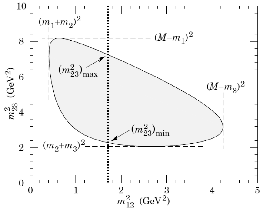
The limits of integration can be determined from the Dalitz plot [51], which leads to the following formula for the decay rate of A into
| (427) |
Integrating over , we obtain
| (428) |
The range of is determined by the value of when is parallel or antiparallel to as follows [51]
| (429) | ||||
| (430) |
where and are the energies of particles and , respectively, in the rest frame,
| (431) |
Finally, the explicit expression for the three-body decay rate for the process is:
| (432) |
where is the corresponding tree-level decay amplitude, and is a symmetrization factor (it is equal to if , and are all different, and equal to for two identical particles in the final state, and equal to for three identical particles in the final state).
Chapter 6 Decay of the pseudoscalar glueball into scalar and pseudoscalar mesons
“The most exciting phrase to hear in science, the one that
heralds new discoveries, is not ‘Eureka’ (I found it), but ‘that’s
funny’…”
Isaac Asimov
27 Introduction
The fundamental symmetry underlying Quantum Chromodynamics (QCD), the theory of strong interactions, is the exact local colour symmetry. As a consequence of the non-Abelian nature of this symmetry the gauge fields of QCD (the gluons) are coloured objects and therefore interact strongly with each other. Because of confinement, one expects that gluons can also form colourless, or ‘white’, states which are called glueballs.
In this chapter we study the decay properties of a pseudoscalar glueball state whose mass lies, in agreement with lattice QCD, between and GeV. Following Ref. [111, 113, 210, 211] we write down an effective chiral Lagrangian which couples the pseudoscalar glueball field (denoted as ) to scalar and pseudoscalar mesons. We can thus evaluate the widths for the decays and where and stand for pseudoscalar and scalar quark-antiquark states. The pseudoscalar state refers to the well-known light pseudoscalars , while the scalar state refers to the quark-antiquark nonet of scalars above 1 GeV: . The reason for the latter assignment is a growing consensus that the chiral partners of the pseudoscalar states should not be identified with the resonances below 1 GeV, see Refs. [78, 108, 110] for results within the extended linear sigma model, see also other theoretical works in Refs. [72, 73, 74, 75, 76, 77, 131, 212, 213, 214, 215, 216, 217] (and refs. therein).
The chiral Lagrangian that we construct contains one unknown coupling constant which cannot be determined without experimental data. However, the branching ratios can be unambiguously calculated and may represent a useful guideline for an experimental search of the pseudoscalar glueball in the energy region between to GeV. In this respect, the planned PANDA experiment at the FAIR facility [218] will prove fruitful, since it will be capable of scanning the mass region above 2.5 GeV. The experiment is based on proton-antiproton scattering, thus the pseudoscalar glueball can be directly produced as an intermediate state. We shall therefore present our results for the branching ratios for a putative pseudoscalar glueball with a mass of 2.6 GeV.
In addition to the vacuum properties of a pseudoscalar glueball, we describe (to our know-ledge [124, 125, 126, 127] for the first time) the interaction of with baryons: we introduce the chiral effective Lagrangian which couples to the nucleon field and its chiral partner. This Lagrangian describes also the proton-antiproton conversion process , which allow us to study the decay of a pseudoscalar glueball into two nucleons.
Additionally, it is possible that the pseudoscalar glueball has a mass that is slightly lower than the lattice-QCD prediction and that it has been already observed in the BESIII experiment where pseudoscalar resonances have been investigated in decays [219, 220, 221]. In particular, the resonance which has been clearly observed in the channel represents a good candidate, because it is quite narrow ( MeV) and its mass lies just below the lattice-QCD prediction. For this reason we repeat our calculation for a pseudoscalar glueball mass of GeV, and thus make predictions for the resonance , which can be tested in the near future.
28 The effective Lagrangian with a pseudoscalar glueball
In this section we consider an chiral Lagrangian which describes the interaction between the pseudoscalar glueball and (pseudo)scalar mesons. We calculate the decay widths of the pseudoscalar glueball, where we fixed its mass to 2.6 GeV, as predicted by lattice-QCD simulations, and take a closer look at the scalar-isoscalar decay channel. We present our results as branching ratios which are relevant for the future PANDA experiment at the FAIR facility.
We introduce a chiral Lagrangian which couples the pseudoscalar glueball with quantum numbers to scalar and pseudoscalar mesons as in Refs. [111, 124, 125, 126, 127, 211]
| (433) |
where is a (unknown) dimensionless coupling constant.
| (434) |
represents the multiplet of scalar and pseudoscalar quark-antiquark states, and are the generators of the group . In the present case the explicit representation of the scalar and pseudoscalar mesons reads [110, 116]:
| (435) |
Let us consider the symmetry properties [9, 10] of the effective Lagrangian (433). The pseudoscalar glueball consists of gluons and is therefore a chirally invariant object. Under chiral transformations the multiplet transforms as where is an element of the group of matrices. Performing these transformations on the determinant of it is easy to prove that this object is invariant under , but not under the axial transformation,
This is in agreement with the so-called axial anomaly. Consequently the effective Lagrangian (433) possesses only an symmetry. Further essential symmetries of the strong interaction are the parity and charge conjugation . The pseudoscalar glueball and the multiplet transform under parity as
Performing the discrete transformations and
on the effective Lagrangian (433) leave it
unchanged. In conclusion, one can say that the symmetries of the
effective Lagrangian (433) are in agreement with the
symmetries of the QCD Lagrangian. The rest of the mesonic
Lagrangian which describes the interactions of and also
includes (axial-)vector degrees of freedom is presented in Sec. 16.
28.1 Implications of the interaction Lagrangian
We have to consider that when spontaneous chiral symmetry breaking occurs and the scalar-isoscalar fields condense. When this breaking takes place, we need to shift the scalar-isoscalar fields by their vacuum expectation values and ,
| (436) |
and
| (437) |
In addition, when (axial-)vector mesons are present in the Lagrangian, one also has to ‘shift’ the (axial-)vector fields and to define the wave-function renormalization constants of the (pseudo)scalar fields:
| (438) |
where runs over the four kaonic fields and Once the field transformations in Eqs. (437) and (438) have been performed, the Lagrangian (433) contains the relevant tree-level vertices for the decay processes of , and takes the form [124]:
| (439) |
which is used to determine the coupling of the field to the scalar and pseudoscalar mesons.
29 Field assignments
The assignment of the quark-antiquark fields in Eq.
(433) or (435) is as follows:
(i) In the pseudoscalar sector the fields and
represent the pions
and the kaons, respectively [23]. The bare fields and are the non-strange and
strange
contributions of the physical states and [23]:
| (440) |
where is the mixing angle
[110]. Using other values for the mixing angle, e.g. [159] or
, as determined by the KLOE Collaboration
[92], affects the presented results only marginally.
In the effective Lagrangian (433) there exists a mixing
between the bare pseudoscalar glueball and both
bare fields and , but due to the large mass
difference between the pseudoscalar glueball and the pseudoscalar
quark-antiquark fields, it turns out that this mixing is very small
and is therefore negligible.
(ii) In the scalar sector the field corresponds to
the physical isotriplet state and the scalar kaon
field to the physical isodoublet state
[23]. The field
is the bare
nonstrange isoscalar field and it corresponds to the resonance
[110, 80]. The field
is the bare strange isoscalar field and
the debate about its assignment to a physical state is still
ongoing; in a first approximation it can be assigned to the
resonance [110] or [80].
(Scalars below 1 GeV are predominantly tetraquarks or mesonic
molecular states, as seen in Refs. [212, 213, 214, 222, 216, 223, 224, 225, 226, 227, 228],
which are not considered here). In order to properly take into
account mixing effects in the scalar-isoscalar sector, we have
also used the results of Refs. [79, 80]. The mixing takes
the form:
| (441) |
where is a scalar glueball field which is absent in this study and is an orthogonal (3 3) matrix which has three solutions. The solution 1 and 2 from Ref. [79] is:
| (442) |
| (443) |
and the solution 3 from Ref. [80]:
| (444) |
In the solution 1 of Ref. [79] the resonance
is predominantly an state, the resonance is
predominantly a glueball, and is predominantly a
strange state. In the solution 2 of Ref. [79]
and in the solution of Ref. [80] the resonance
is still predominantly a nonstrange state,
but is now predominantly a glueball, and
predominantly a strange state.
Note that the experimental values of the fields are used, which are summarized with the numerical values of the renormalization constants [110], the vacuum expectation values of and which are (212) and (213), respectively, and the decay constants of pion ( ) and kaon () [51] in the following Table 9
| Observable | Experiment([51])[MeV] | constants | Value |
|---|---|---|---|
| 1.709 | |||
| 1.604 | |||
| 1.001 | |||
| 1.709 | |||
| 1.539 | |||
| 158 MeV | |||
| 138 MeV | |||
| 92.2 MeV | |||
| 110 MeV |
30 Decay widths of a pseudoscalar glueball into (pseudo)scalar mesons
The chiral Lagrangian (439) describes the two- and three-body decays of a pseudoscalar glueball, , into scalar
and pseudoscalar mesons. All the decay rates depend on the unknown
coupling constant . The decay widths
for the two- and three-body decays of a pseudoscalar glueball are listed in the following:
Firstly, let us list the two-body decay widths for a pseudoscalar glueball, . Performing the two-body decay-width calculation Eq.(407), the decay widths for every channel can be obtain as follows:
| (445) |
| (446) |
| (447) |
| (448) |
| (449) |
| (450) |
Secondly, let us turn to the three-body decay widths for a pseudoscalar glueball, . We use the three-body decay-width expression Eq.(432), which reads in the present case for the decay of into three pseudoscalar mesons and ,
| (451) |
The quantities are the masses of
and ,
is the tree-level decay
amplitude, and is a symmetrization factor (it
is equal to if , and
are all different, equal to for two identical
particles in the final state, and equal to for three identical particles in the final state). The decay channels can be obtained as follows:
(1) The full decay width into the channel results from the sum
| (452) |
with the modulus squared decay amplitude
where and .
(2) The full decay width into the channel results from the sum
| (453) |
with the modulus squared decay amplitude
where , and .
(3) The decay width into the channel has as modulus squared decay amplitude
where and the
symmetrization factor .
(4) The decay width into the channel has as modulus squared decay amplitude
where , and the
symmetrization factor .
(5) The decay width into the channel has as modulus squared decay amplitude
where , and the
symmetrization factor .
(6) The full decay width into the channel is computed from the sum
| (454) |
with the modulus squared decay amplitude
where and .
(7) The full decay width into the channel is computed from the sum
| (455) |
with the modulus squared decay amplitude
where and .
(8) In the case one has:
where and . Then:
| (456) |
The full decay width into the channel results from the sum
| (457) |
There exists an interesting and subtle issue: a decay channel
which involves some scalar states which decay further into two
pseudoscalar ones. For instance, decays into . There are then two possible decay
amplitudes for the process : one is
the direct decay mechanism reported in Table 6.2, and the other is
the decay chain .
The immediate question is, if interference effects emerge which
spoil the results presented in Table 10 and 11. Namely, simply performing the sum of the direct three-body decay
(Table 10) and the corresponding two-body decay (Table 11) is
not correct.
We now describe this point in more detail using the neutral
channel as an
illustrative case. To this end, we describe the coupling
to via the Lagrangian
| (458) |
The coupling constant GeV is obtained by using the experimental value for the total decay width MeV [23]. The full amplitude for the process will result from the sum
| (459) |
Thus for the decay width we obtain
| (460) |
where is the sum of all interference terms. We can then investigate the magnitude of the mixing term , and thus the error incurred when it is neglected. The explicit calculation for the case gives a relative error of
| (461) |
Present results from the model in Ref. [110] show that : the estimates presented in Ref. [124] may be regarded as upper limits. We thus conclude that the total error for the channel is not large and can be neglected at this stage. However, in any future, more detailed and precise theoretical calculation, these interference effects should also be taken into account.
30.1 Results
The branching ratios of for the decays into three pseudoscalar mesons are reported in Table 10 for both choices of the pseudoscalar masses, and GeV (relevant for PANDA and BESIII experiments, respectively). The branching ratios are presented relative to the total decay width of the pseudoscalar glueball .
| Quantity | Case (i): GeV | Case (ii): GeV |
|---|---|---|
Next we turn to the decay process The results, for both choices of are reported in Table 11 for the cases in which the bare resonance is assigned to or to
| Quantity | Case (i): GeV | Case (ii): GeV |
|---|---|---|
Note that the results are presented as branching ratios because of the as of yet undetermined coupling constant . Concerning the decays involving scalar-isoscalar mesons, one should go beyond the results of Table 11 by including the full mixing pattern above 1 GeV, in which the resonances and are mixed states of the bare quark-antiquark contributions , , and a bare scalar glueball field This mixing is described by an orthogonal matrix, see Eq. (441) [72, 73, 74, 75, 76, 77, 78, 79, 80, 81, 82]. In view of the fact that a complete evaluation of this mixing in the framework of our chiral approach has not yet been done, we use the two solutions for the mixing matrix of Ref. [79] and the solution of Ref. [80] in order to evaluate the decays of the pseudoscalar glueball into the three scalar-isoscalar resonances and . In all three solutions is predominantly described by the bare configuration , but the assignments for the other resonances vary: in the first solution of Ref. [79] the resonance is predominantly gluonic, while in the second solution of Ref. [79] and the solution of Ref. [80] the resonance has the largest gluonic content. The results for the decay of the pseudoscalar glueball into scalar-isoscalar resonances are reported in Table 12.
| Quantity | Sol. 1 of Ref. [79] | Sol. 2 of Ref. [79] | Sol. of Ref. [80] |
|---|---|---|---|
In Fig. 7 we show the behavior of the total decay width as function of the coupling constant for both choices of the pseudoscalar glueball mass. (We assume here that other decay channels, such as decays into vector mesons or baryons are negligible.) In the case of GeV, one expects from large- considerations that the total decay width MeV. In fact, as discussed in the Introduction, the scalar glueball candidate is roughly MeV broad and the tensor candidate is even narrower. In the present work, the condition MeV implies that . Moreover, in the case of GeV for which the identification has been made, we can indeed use the experimental knowledge of the full decay width [ MeV [219, 220, 221]] to determine the coupling constant to be . (However, we also refer to the recent work of Ref. [229], where the possibility of a broad pseudoscalar glueball is discussed.)

Some comments are in order:
(i) The results depend only slightly on the glueball mass. Thus, the two columns of Table 10 and 11 are similar. It turns out that the channel is the dominant one (almost 50%), and also that the and channels are sizable. On the other hand, the two-body decays are subdominant and reach only 20% of the full mesonic decay width.
(ii) The decay of the pseudoscalar glueball into three pions vanishes:
| (462) |
This result represents a further testable prediction of our approach.
(iii) The decays of the pseudoscalar glueball into a scalar-isoscalar meson amount only to of the total decay width. Moreover, the mixing pattern in the scalar-isoscalar sector has a negligible influence on the total decay width of Nevertheless, in the future it may represent an interesting and additional test for scalar-isoscalar states.
(iv) Once the shifts of the scalar fields have been performed, there are also bilinear mixing terms of the form and which lead to a non-diagonal mass matrix. In principle, one should take these terms into account (in addition to the already-mentioned mixing) and solve a three-state mixing problem in order to determine the masses of the pseudoscalar particles. This will also affect the calculation of the decay widths. However, due to the large mass difference of the bare glueball fields in contrast to the other quark-antiquark pseudoscalar fields, the mixing of turns out to be very small in the present work, and can be safely neglected. For instance, it turns out that the mass of the mixed state which is predominantly glueball is (at most) just GeV larger than the bare mass GeV.
(v) If a standard linear sigma model without (axial-)vector mesons is studied, the replacements need to be performed. Most of the results of the branching ratios for the three-body decay are qualitatively (but not quantitatively) similar to the values of Table 10 (variations of about -). However, the branching ratios for the two-body decay change sizably w.r.t. the results of Table 11. This fact shows once more that the inclusion of (axial-)vector degrees of freedom has sizable effects also concerning the decays of the pseudoscalar glueball.
(vi) In principle, the three-body final states for the decays shown in Table 10 can also be reached through a sequential decay from the two-body final states shown in Table 11, where the scalar particle further decays into , for instance, . There are then two possible decay amplitudes: One from the direct three-body decay, and one from the sequential decay, which have to be added coherently before taking the modulus square to obtain the total three-body decay width. Summing the results shown in Table 10 and 11 gives a first estimate (which neglects interference terms) for the magnitude of the total three-body decay width. We have verified that the correction from the interference term to this total three-body decay width in a given channel is at most of the order of % for GeV and for GeV. For a full understanding of the contribution of the various decay amplitudes to the final three-body state, one needs to perform a detailed study of the Dalitz plot for the three-body decay.
31 Interaction of a pseudoscalar glueball with nucleons
In this section we compute the decay width of the pseudoscalar
glueball into a nucleon and an antinucleon and we present the result as a
branching
ratio to remove the effects of the undetermined coupling constant.
A Lagrangian of the interaction of a pseudoscalar glueball with the baryon fields and [126, 230] is
| (463) |
This interaction Lagrangian (463) describes the fusion of a proton and an antiproton, which is hermitian and invariant under , parity (), and charge conjugation as proved in Ref. [230]. Now let us write the interaction Lagrangian with the physical fields and which refer to the nucleon and its partner [230] , respectively. By substituting Eqs. (180-183) into Eq.(463), we obtain
| (464) |
We consider first the pseudoscalar field and the nucleon fields and as confined in a cube of length and volume . The four-momenta of , , and are denoted as , , and , respectively: From Quantum Mechanics it is known that their 3-momenta are quantized as and . Using a Fourier transformation the field operators [230] can be obtained as
| (465) |
| (466) |
and
| (467) |
where, as known from Quantum Field Theory, the glueball and the two fermionic fields were
decomposed in terms of annihilation and creation operators, ,
, and , ,
respectively.
In Eq. (464) the coupling constant
cannot be determined, but it is easy to calculate the ratio of the
decay of the pseudoscalar glueball into a
nucleon and an antinucleon and of the decay into and [230],
| (468) |
31.1 Decay of a pseudoscalar glueball into two nucleons
Let us calculate the decay process of which is described by the first term in Eq.(464),
| (469) |
The resonance represents the initial state
| (470) |
whereas the final state is
| (471) |
The corresponding matrix element of the scattering matrix reads
| (472) |
We now calculate the expectation value in terms of the initial and final states:
| (473) |
Inserting Eqs. (465), (466), (467), and (469) into (473) and performing a time-ordered product of creation and annihilation operators [230] we obtain
| (474) |
We therefore obtain
| (475) |
where is the volume of the ‘box’ which contains the fields and is the invariant amplitude which is given by
| (476) |
To find the lifetime of we have to take the square of the amplitude, which is the probability for the process,
| (477) |
where
This is proved in Sec.5.3. The probability for the decay, when the two particles have momenta between and , is given by
| (478) |
By integrating over all possible final momenta, summing over all final spin orientations and division by , one can calculate the decay rate as
| (479) |
In the rest frame of the decaying particle, , one finds
| (480) |
Solving the integral over (by using the Dirac delta function) we are left with
| (481) |
We can write
| (482) |
where
| (483) |
is the modulus of the momenta of the outgoing particles. Using the spherical coordinates, and solving the integral over , one obtains the decay rate as
| (484) |
For the computation of , one should use the following two identities [230] :
| (485) |
and
| (486) |
The averaged modulus squared amplitude will thus be
where
Then we obtain the final result of the decay rate as follows
| (487) |
Similarly, we now proceed to calculate the rate for the decay process , which is described in Eq.(464) by the term
| (488) |
The corresponding matrix element can be obtained by
| (489) |
which can be written as:
| (490) |
where
| (491) |
The decay rate of the pseudoscalar glueball into is obtained as
| (492) |
where
| (493) |
which is proved in Ref. [230]. The averaged modulus squared decay amplitude is
We obtain the final result of the decay width as
| (495) |
The mass of the nucleon and its partner are MeV and MeV, respectively [23], whereas the mass of the lightest pseudoscalar glueball is predicted from lattice calculations to be about GeV. The moduli of the momenta of the outgoing particles are MeV and MeV. From Eq.(487) and Eq.(495) we obtain the branching ratio (468) of the pseudoscalar glueball decay processes and [126, 230]:
| (496) |
which can be tested by the upcoming PANDA experiment at the FAIR facility in Darmstadt.
Chapter 7 Decay of open charmed mesons
32 Introduction
Charm physics is an experimentally and theoretically active field of hadronic physics [231]. The study of strong decays of the heavy mesons into light pseudoscalar mesons is useful to classify the charmed states. In this chapter, which is based in the paper [119], we study the strong OZI-dominant decays of the open heavy charmed states into light mesons. In this way, our model acts as a bridge between the high- and low-energy sector of the strong interaction. It turns out that the OZI-dominant decays are in agreement with current experimental results, although the theoretical uncertainties for some of them are still very large. Nevertheless, since our decay amplitudes depend on the parameters of the low-energy sector of the theory, there seems to be an important influence of chiral symmetry in the determination of the decay widths of charmed states. As a by-product of our analysis, we also obtain the value of the charm-anticharm condensate and the values of the weak decay constants of mesons. Moreover, in the light of our results we shall discuss the interpretation of the enigmatic scalar strange-charmed meson and the axial-vector strange-charmed mesons and [59, 189, 190, 191]. We show the explicit form of open-charmed decay widths which were obtained from the Lagrangian (163) at tree level. The formulas are organized according to the type of decaying particle. The precise description of the decays of open charmed states is important for the CBM experiment at FAIR.
33 Decay widths of open-charmed scalar mesons
In this section we study the phenomenology of the open charmed
mesons in the scalar sector. The Lagrangian (163)
contains two open charmed scalar mesons which are and
. The neutral scalar state and the
charged decay into , while the
strange-charmed state decays into . The corresponding
interaction Lagrangian from Eq.(163) for the
nonstrange-charmed meson with and the
strange-charmed meson with has the same structure, as we
shall see below. Then, we shall calculate the general decay width
of a scalar
state in this case.
We consider a generic decay process of a scalar state into two
pseudoscalar states , i.e., . The interaction Lagrangian for
the neutral scalar state will be given in the following general
simple form:
| (497) |
Firstly, to calculate the decay amplitude for this process we denote the momenta of as respectively. Then, (upon substituting for the decaying particles and for the decay products) we obtain the Lorentz-invariant decay amplitude as
| (498) |
Using energy momentum conservation on the vertex, , we obtain
| (499) |
In the decay process, the two pseudoscalar mesons and are on-shell; therefore and . Moreover,
| (500) |
Therefore, the decay amplitude (499) can be written as
| (501) |
The decay width then reads
| (502) |
A non-singlet scalar field will posses also charged decay channels. We then have to consider the contribution of the charged modes from the process to the full decay width. By multiplying the neutral-mode decay width of Eq.(502) with an isospin factor , we obtain
| (503) |
The full decay width can be written as
| (504) |
where is determined from isospin deliberations, or from the interaction Lagrangian of a given decay process.
Note that usually the contribution of the charged modes, is twice
the contribution of the neutral modes, which, as we will see in
the explicit interaction Lagrangian below, leads us to write the
general decay width of into charged modes,
, as follows:
| (505) |
Using this general structures of the decay process of a scalar into two pseudoscalar states, , in the following we compute the decay width of the nonstrange-charmed scalar state into and the strange-charmed scalar state into .
33.1 Decay Width
Firstly, we study the phenomenology of the scalar doublet charmed mesons which are assigned to . These open-charmed mesons are known to decay into [119, 120, 122]. The corresponding interaction Lagrangian from Eq.(163), for only the neutral and positively-charged components (the other ones like possess analogous forms) reads
| (506) |
where the coefficients read
| (507) | ||||
| (508) | ||||
| (509) | ||||
| (510) | ||||
| (511) | ||||
| (512) | ||||
| (513) | ||||
| (514) |
Note that the parameters and are imaginary as shown in Eqs. (4.48) and (4.49), respectively, which means that the coefficients containing the imaginary unit are real. Furthermore the wave-function renormalisation factors and are equal, as well as the parameters and (for isospin symmetry reasons), which leads to
In the interaction Lagrangian (506), the considered decays are that of the neutral state and the positively charged state . Both have two relevant decay channels .
Firstly, let us focus on the decay of which decays into neutral modes and charged modes . The explicit expression for the decay process is similar to Eq.(497) as seen in Eq.(506); when using Eq.(502) upon identifying the mesons with the scalar meson , and the pseudoscalar mesons as and , respectively. The coefficients and refer to and , respectively. We then obtain as follows:
| (515) |
The decay width for has the same expression as (515) but is multiplied by an isospin factor 2, which can be seen in Eq.(505). All the parameters entering Eqs.(515) have been fixed as presented in Tables 4.1, 4.2, and 4.3. The value of is then determined as follows:
| (516) | ||||
| (517) |
Now let us turn to the positively charged scalar state which decays into and . The explicit expression for the decay process is also similar to Eq.(497) as seen in Eq.(506), when using Eq.(502) (upon identifying the mesons with and , respectively). One may proceed in a similar manner for the decay width of , where an overall isospin factor is also present. Then we obtain the value for :
| (518) | ||||
| (519) |
33.2 Decay Width
We turn here to the phenomenology of the scalar state which is assigned to . This open strange-charmed meson decays into and [119] as known from [51]. The corresponding interaction Lagrangian from Eq.(163) reads
| (520) |
with the following coefficients
| (521) |
| (522) |
| (523) |
| (524) |
As seen in Eq.(520) the explicit expression of has a form analogous to that of for isospin symmetry reasons. The decay width of the process is obtained from Eq.(504) when using Eq.(501) upon identifying and with and and upon replacing . The decay width for the process has an analogous analytic expression. The full decay width of with a mass of about MeV into [119], see Table 7, is then
34 Decay widths of open-charmed vector mesons
In this section we describe the phenomenology of open-charmed vector mesons . The neutral state is assigned to while the positively charged state to . These resonances decay into two pseudoscalar states [51]. Let us now consider the decay of a vector state into two pseudoscalar states , i.e., , in general. The general simple form of the interaction Lagrangian, as obtained from Eq.(163), reads
| (525) |

We denote the momenta of , , and as , , and , respectively, and compute the decay amplitude for this process. We consider the polarization vector for the vector state. Then, upon substituting for the decaying particle and for the decay products, we obtain the following Lorentz-invariant scattering amplitude from the Lagrangian (525):
| (526) |
with
| (527) |
where denotes the
vertex.
The calculation of the decay width requires the determination of
the modulus square of the scattering amplitude. The scattering amplitude
in Eq. (526)
depends on the polarization vector .
For a general scattering amplitude, one has to calculate
of a process containing one vector state with
mass . The calculation reads as follows:
| (528) | ||||
| (529) |
where
| (530) |
Eq.(529) contains the metric tensor . Note that, if the vector particle decays, then in the rest frame of the decaying particle and thus
| (531) |
Therefore, we have to calculate the squared vertex using Eq.(527):
| (532) |
Now let us compute the squared vertex at rest (also using Eq. (527)):
| (533) |
We can then write Eq.(534) in a slightly different (but equivalent) form, by inserting Eq.(535) into Eq. (529) as follows:
| (537) |
| (538) |
The decay width for a vector meson decaying into two pseudoscalar mesons (as obtained from Eq. (525) can be computed with the following formula:
| (539) |
where is an isospin factor and the modulus square of the decay amplitude is given in Eq. (538) or, equivalently, Eq. (534). Now let us apply this result to calculate the decay width of the vector meson into from the Lagrangian (163).
34.1 Decay Width
The interaction Lagrangian from Eq.(163) reads
| (540) |
with the following coefficients
| (541) | ||||
| (542) | ||||
| (543) |
Note that the Lagrangian in Eq. (540) contains the
parameter combinations , ,
and and their complex conjugates. Thus, it is
certain that the Lagrangian is hermitian; so we obtain
.
In the following we will focus only on the decays
and ,
where the corresponding decay of and
yields the same result due to isospin
symmetry.
The interaction Lagrangian (540) has two decay channels for the neutral charmed-vector meson , which are and . We have to note that the decay of into is impossible because, in this situation, the sum of the decay product masses is larger than the mass of the decay particle, so
This result shows very good agreement with the experiment result: experimentally it is not seen, as listed by the Particle Data Group [51]. Then the decay of the neutral state into the neutral modes is the only possible decay in the eLSM (163). To compute , we use Eqs. (538) and (539) upon identifying with and the coefficients with , respectively. We then obtain the corresponding expression
| (544) |
The parameters entering Eq.(540) have been determined uniquely from the fit (see Tables 4.1, 4.2, and 4.3). Therefore we can calculate the value of the decay width immediately:
| (545) |
where the experimental value reads
MeV as listed in Ref. [51].
Now let us turn to the phenomenology of the positively charged state , which can decay into and . The decay width of the channel has an analogous analytic expression as , which is described in Eq.(544), whereas concerning the decay Eq. (544) holds upon multiplication with an isospin factor . We then obtain the following results:
| (546) |
| (547) |
35 Decay widths of open charmed axial-vector mesons
In this section we turn to the study of the phenomenology of axial-vector charmed mesons, i.e., the two- and three-body decays of and the two-body decays of the strange . The nonstrange-charmed field corresponds to the resonances while the strange-charmed doublet is assigned to the resonance . Firstly let us focus on the two-body decays of the axial-vector charmed mesons . The nonstrange-charmed decays into vector-charmed and light pseudoscalar mesons, , while the strange-charmed doublet decays into , which also contains a vector-charmed meson and a light pseudoscalar meson. Therefore, both decays have the same structure of the corresponding expression for the decay amplitude. This leads us to consider the general case of the two-body decay process of an axial-vector meson into a vector and a pseudoscalar state , i.e., . The following interaction Lagrangian describes the decay of the axial-vector state into neutral modes:
| (548) |

Let us study a generic decay process of the form . The 4-momenta of , and are denoted as , and , respectively. We have to consider the corresponding polarization vectors because there are two vector states involved in the decay process , i.e., and . These we denote as for and for . Using the substitutions for the decaying particle and for the decay products, we obtain the Lorentz-invariant scattering amplitude as follows:
| (549) |
with
| (550) |
where denotes the
vertex.
It will be necessary to determine the modulus square of the scattering amplitude in order to calculate the decay width. We note that the scattering amplitude in Eq. (549) depends on the polarization vectors and . Therefore, it is necessary to calculate the average of the modulus squared amplitude for all polarization values. Let us denote the masses of the vectors states and as and , respectively. Then the averaged modulus squared amplitude is determined as follows:
| (551) |
Given that
| (552) |
[an analogous equation holds for ], we obtain from Eq. (551):
| (553) |
which contains the metric tensor . The decay width for the process then reads
| (554) |
Note that a non-singlet axial-vector field will in general also possess charged decay channels. Therefore, in addition to the decay process considered in Eq. (554), we must consider the contribution of the charged modes from the process to the full decay width. Then the full decay width is obtained as
Using Eq.(553) we obtain the two-body decay width of vector meson, Eq.(554), as follows:
| (555) |
where the quantities , , and are the four-momenta of , , and in the rest frame of , respectively. The following kinematic relations hold:
The terms entering in Eq. (555) are given by
| (556) |
| (557) |
| (558) |
with and .
35.1 Two-body decay of
We present the relevant interaction Lagrangian for the nonstrange axial-vector meson which is a light-heavy quark and is assigned to . This Lagrangian describes only the two-body decays of this state, and is given as:
| (559) |
with the following coefficients
| (560) | ||||
| (561) |
From the interaction Lagrangian (559) we obtain that the neutral state of decays into and that the positively charged state decays into (see below). The interesting point is that the decays and (although kinematically allowed) do not occur in our model; because there is no respective tree-level coupling. This is in agreement with the small experimental upper bound. Improvements in the decay channels of could be made by taking into account also the multiplet of pseudovector quark-antiquark states. In this way, one will be able to evaluate the mixing of these configurations and describe at the same time the resonances and .
35.1.1 Decay Width
The decay width of into is given by Eq. (555) upon substituting the fields and with and respectively. One may do likewise for the decay width of into , but in this case it is necessary to multiply the expression by an isospin factor Given that all parameters entering Eqs. (555, 560, 561) are known from Tables 4.1, 4.2, and 4.3, we consequently obtain the following value of the decay width of into
| (562) |
Experimentally the decay width of into has been observed.
35.1.2 Decay Width
One can proceed in a similar manner for the state, but in this case we set , and in Eq. (555). We obtain the following value of the decay width
| (563) |
35.2 Decay Width
Now we turn to the three-body decays of the open axial-vector nonstrange charmed meson which decays into three pseudoscalar mesons, . The relevant interaction Lagrangian can be written in a single equation as follows:
| (564) |
with the coefficients
| (565) | ||||
| (566) | ||||
| (567) | ||||
| (568) | ||||
| (569) |
As seen in the Lagrangian (564) there are three relevant channels for the neutral state which are , , and . The positive state also has three relevant channels due to , , and .
35.2.1 Decay Width
The Lagrangian (564) allows us to calculate the decay width for the process . Firstly let us focus on the three body-decay of the neutral state into . We denote the momenta of and as , and . A vector state is involved in this decay process. We then consider the corresponding polarization vector for , and substitute for the decaying particle and for the decay products. We straightforwardly obtain the following scattering amplitude from the Lagrangian (564):
| (571) |
where is the vertex following from the relevant part of the Lagrangian,
| (572) |
In order to calculate the decay width of we need to calculate the averaged modulus squared decay amplitude from Eq.(571):
| (573) |
where
| (574) |
| (575) |
where , , , and are the four-momenta of , , , and in the rest frame of , respectively. In this frame,
The quantities refer to the mass of , respectively. Using Eq.(451) the decay width for the process can be obtained as
| (576) |
The decay of the neutral states for the processes and has the same formula as in Eq. (576), only in this case it is multiplied by an isospin factor as given by the Lagrangian (564). We then get
| (577) |
35.2.2 Decay Width
The scattering amplitudes for the processes and differ markedly from the previous processes for the three-body decay of , as can be seen from the interaction Lagrangian (564). Thus, we study the decay widths for these channels differently. Let us firstly focus on the decay width of the neutral state into , which has the same expression as for the decay process . To write the scattering amplitude for we denote the momenta of , and as , and . For the meson , we consider the polarization vector and substitute for the decaying particle and for the outgoing particles. We then obtain the following decay amplitude from the Lagrangian (564):
| (579) |
where the vertex is
| (580) |
The averaged modulus squared amplitude has the same general formula as in Eq.(573), with substituting the vertices ,
| (581) |
The decay width reads
| (582) |
where the quantities and refer to the masses for the fields and , respectively, and the kinematic relations
All the parameters entering Eq.(582) are fixed and listed in the Tables 4.1 and 4.3. Consequently we obtain the decay width of into :
| (583) |
The decay of the charged state into has an analogous expression and is
| (584) |
This decay is observed experimentally.
35.3 Decay Width
As a last step we turn to the strange-charmed axial-vector state which is assigned to . This resonance decays into and in the model (163), whereas kinematically the decay to is not allowed. This is in agreement with experimental data in which the decays and are not seen (as stated by the PDG [51]). The interaction Lagrangian from Eq. (163) reads
| (585) |
with the following coefficients
| (586) | ||||
| (587) |
According to the interaction Lagrangian, decays into the channels and . The formula for the decay widths and is as in Eq. (555), when setting and replacing the vertex by the following vertex :
| (588) |
The parameters are fixed and presented in Tables 4.1, 4.2, and 4.3. We then obtain the decay width into as
| (589) |
whereas MeV.
36 Weak decay constants of Charmed mesons
In this subsection we evaluate the weak decay constants of the pseudoscalar mesons , and . Their analytic expressions read [see Appendix A and also Ref. [118, 119, 122]]
| (590) | ||||
| (591) | ||||
| (592) |
Using the parameters of the fit we obtain
| (593) | ||||
| (594) | ||||
| (595) |
The experimental values MeV and MeV [51] show a good agreement for and a slightly too large theoretical result for . The quantity is in fair agreement with the experimental value MeV [232] as well as with the theoretical result MeV obtained in Ref. [233]. These results show that our determination of the condensate is reliable (even if the theoretical uncertainty is still large).
37 Summary
We summarize the results of the (OZI-dominant) strong decay widths
of the resonances , and in
Table 7.1. For the calculation of the decay widths we
have used the physical masses listed by the PDG [51]. This is necessary
in order to have the correct phase space. With the exception of
all values are in reasonable
agreement with the mean experimental values and upper bounds.
Although the theoretical uncertainties are still large and the
experimental results are not yet well known, the qualitative
agreement is anyhow interesting if one considers that the decay
amplitudes depend on the parameters of the three-flavour version of
the model determined in Ref. [110]. Note that the
theoretical errors have been calculated by
taking into account the uncertainty in the charm condensate MeV. The lower theoretical value corresponds to
MeV, while the upper one to
MeV. The explicit expressions
for the decay widths are reported in the previous.
Here we do not study the decay of other (hidden and open) charmed
states because we restrict ourselves to OZI-dominant processes.
The study of OZI-suppressed decays which involve the large-
suppressed parameters and is left for the next chapter. There, also the decays of the well-known charmonium states
(such as and ) will be investigated.
| Decay Channel | Theoretical result [MeV] | Experimental result [MeV] |
|---|---|---|
| seen; full width | ||
| seen; full width: | ||
| seen; | ||
| not seen | ||
| seen; full width: | ||
| seen | ||
| seen | ||
| not seen; | ||
| seen; full width: | ||
| seen | ||
| seen | ||
| not seen; | ||
| seen; full width | ||
| not seen | ||
| not seen |
Table 7.1: Decay widths of charmed mesons.
The following comments are in order:
(i) The decay of into has a very large theoretical error due to the imprecise determination of . A qualitative statement is, however, possible: the decay channel is large and is the only OZI-dominant decay predicted by our model. This decay channel is also the only one seen in experiment (although the branching ratio is not yet known). A similar discussion holds for the charged counterpart .
(ii) The decay widths of the vector charmed states and are slightly smaller than the experimental results, but close to the lower bounds of the latter.
(iii) The results for the axial-vector charmed states and are compatible with experiment. Note that the decay into is the only one which is experimentally seen. Moreover, the decays and , although kinematically allowed, do not occur in our model because there is no respective tree-level coupling; this is in agreement with the small experimental upper bound. Improvements in the decay channels of are possible by taking into account also the multiplet of pseudovector quark-antiquark states. In this way, one will be able to evaluate the mixing of these configurations and describe at the same time the resonances and .
(iv) It is interesting that the decays of the vector states and and of the axial-vector states and can be simultaneously described with the same set of (low-energy) parameters. Namely, in the low-energy language these states are chiral partners and the results (even if the experimental knowledge is not yet conclusive and the theoretical uncertainties are still large) show that chiral symmetry is still important in the energy range relevant for charmed mesons.
(v) The decay of the axial-vector strange-charmed is too large in our model when compared to the experimental data of about MeV. This result is robust upon variation of the parameters, as the error shows. We thus conclude that the resonance is not favored to be (predominantly) a member of the axial-vector multiplet (it can be, however, a member of the pseudovector multiplet). Then, we discuss two possible solutions to the problem of identifying the axial-vector strange-charmed quarkonium:
Solution 1: There is a ‘seed’ quark-antiquark axial-vector state above the threshold, which is, however, very broad and for this reason has not yet been detected. Quantum corrections generate the state through pole doubling [223, 225, 226]. In this scenario, is dynamically generated but is still related to a broad quark-antiquark seed state. In this way, the low mass of in comparison to the quark-model prediction [47, 48] is due to quantum corrections [179, 200, 201, 202, 234, 235]. Then, the state , being below threshold, has a very small decay width.
Solution 2: Also in this case, there is still a broad and not yet detected quark-antiquark field above threshold, but solution 1 is assumed not to apply (loops are not sufficient to generate ). The resonance is not a quark-antiquark field, but a tetraquark or a loosely bound molecular state and its existence is not related to the quark-antiquark state of the axial-vector multiplet.
(vi) For the state similar arguments apply. If the mass of this state is above the threshold, we predict a very large ( GeV) decay width into (for example: GeV for a mass of MeV as determined in Table 4.5). Then, the two solutions mentioned above are applicable also here:
Solution 1: A quark-antiquark state with a mass above the threshold exists, but it is too broad to be seen in experiment. The state arises through the pole-doubling mechanism.
Solution 2: Loops are not sufficient to dynamically generate The latter is not a quarkonium but either a tetraquark or a molecular state.
In conclusion, a detailed study of loops in the axial-vector and
scalar strange-charm sector needs to be performed. In the
axial-vector strange-charm sector mixing with a pseudovector
quark-antiquark state should also be included. These tasks go
beyond the tree-level analysis of our work but are an interesting
subject for the future.
Chapter 8 Decay of hidden charmed mesons
38 Introduction
Charmonia exhibit a spectrum of resonances and play the same role for understanding hadronic dynamics as the hydrogen atom [236]. The properties of charmonia are determined by the strong interaction which is undoubtedly one of the most challenging tasks. Since the discovery of the charmonium state with quantum numbers in November 1974 at BNL [42] and at SLAC [41], a significant experimental progress has been achieved in charmonium spectroscopy. As an example of this, the hadronic and electromagnetic transitions between charmonium states and their decays have been measured with high precision with the BESIII spectrometer at the electron-positron collider at IHEP Beijing. Moreover, unconventional narrow charmonium-rich states have been recently discovered in an energy regime above the open-charm threshold by Belle [237, 238, 239, 240] and BaBar [241], which potentially initiates a new area in charmonium spectroscopy. The upcoming PANDA experiment at the research facility FAIR will exploit the annihilation of cooled anti-protons with protons to perform charmonium spectroscopy with an incredible precision.
Recent theoretical developments such as nonrelativistic QCD [242, 243, 244] and heavy-quark effective theory [245], potential models [164, 163], lattice gauge theory [246, 247, 248], and light front quantization have shown the direct connection of charmonium properties with QCD. More details of the experimental and theoretical situation is given in the Ref. [59]. Therefore, we highlight the study of the decays of charmonium states and their mixing with glueballs in the eLSM. The charm quark has been included in the eLSM by its extension from the case [110] to the case [119]. The eLSM has four charmonium states, which are the (pseudo-)scalar ground states and with quantum numbers and as well as the ground-state (axial-)vector and with quantum numbers and [118, 119], respectively. It also includes two glueballs: a scalar glueball (denoted as ) and a pseudoscalar glueball (denoted as ), composed of two glouns. There are two candidates for the scalar glueball which are the resonance (which shows a flavour-blind decay pattern) and the resonance , because its mass is very close to lattice-QCD predictions, and because it is produced in the gluon-rich decay of the , as seen in Refs. [72, 73, 74, 75, 76, 77, 78, 79, 80, 81, 82, 217]. The latter is a mixing between three bare fields: the nonstrange , the hidden-strange , and the scalar glueball . This three-body mixing in the scalar-isoscalar channel was solved in Ref.[83] and generated the physical resonances , and . The last field that was introduced in the eLSM is a pseudoscalar glueball via a term describing the interaction between the pseudoscalar glueball with scalar and pseudoscalar mesons; as seen in chapter 6. The decay channels of the pseudoscalar glueball into scalar and pseudoscalar mesons [124, 125, 126, 127] could potentially be measured in the upcoming PANDA experiment at the FAIR facility [218], which is based on proton-antiproton scattering and has the ability to produce the pseudoscalar glueball in an intermediate state with mass above GeV. The mass of a pseudoscalar glueball predicted by lattice QCD (in the quenched approximation) is about GeV [65, 66, 67, 71].
In the present chapter we study the decay properties of the charmonium states and within the eLSM. The charmonia region is a good one to look for exotics [249, 250]. As seen in Ref. [251, 252, 253], lattice QCD predicts the existence of various glueball states in the charmonium mass region, some of them with exotic quantum numbers which are not possible in a state. We then obtain the scalar glueball (due to the decay of ) and the pseudoscalar glueball (due to the decay of ). We calculate the decay width of the charmonium state into a pseudoscalar glueball (this decay is allowed in the channel ), with a mass of GeV predicted by lattice QCD and repeat it with a mass of GeV, as observed in the BESIII experiment where pseudoscalar resonances have been investigated in decays [219, 220, 221]. Particularly, we consider the resonance, since its mass lies just below the lattice-QCD prediction. Mixing phenomena, although believed to be smaller than in the light mesonic sector, can occur also between charmonia and glueballs with the same quantum numbers [254, 255]. The parameters have been used in the strange-nonstrange investigation [110] (which are discussed in chapter 3), whereas the three parameters related to the charm sector have been fixed in chapter 4 through a fit including the masses of charmed mesons. There are two parameters, , which had zero values in the previous case (), but in the present chapter this should be re-evaluated, as the decay widths of depend on their values. For instance, there is a mixing between a scalar glueball with the charmonium state , but we neglect it in our evaluation because it is expected to be small. We compute instead the mixing angle between the pseudoscalar glueball (with a mass of GeV) with .
39 Decay of the scalar charmonium state
In this section we study the decay properties of
the scalar ground-state charmonium in the eLSM,
via computing the decay width of this charmonium state into
(axial-)vector and
(pseudo)scalar mesons and a scalar glueball as well. As a result of the study discussed in Ref.[83], the resonance is predominantly a scalar glueball.
The terms in the eLSM relevant for the decay of are
| (596) |
These terms contain the decay channels of the charmonium state into (pseudo)scalar and (axial-)vector mesons as well as a scalar glueball . The full Lagrangian (163) is presented in chapter 2. The term denoted as is the dilaton Lagrangian which describes the scalar dilaton field which is represented by a scalar glueball with quantum numbers , and emulates the trace anomaly of the pure Yang-Mills sector of QCD [110, 111, 112, 113, 151, 114, 115]:
| (597) |
The energy scale of low-energy QCD is described by the dimensionful parameter which is identical to the minimum of the dilaton potential, (). The scalar glueball mass has been evaluated by lattice QCD which gives a mass of about (1.5-1.7) GeV [65, 66, 67, 71, 256]. The dilatation symmetry or scale invariance, , is realized at the classical level of the Yang-Mills sector of QCD and explicitly broken due to the logarithmic term of the potential in Eq. (597). This breaking leads to a non-vanishing divergence of the corresponding current:
| (598) |
The importance of including the scalar glueball in the eLSM is to
incorporate dilatation invariance meson mass terms. Note that the scalar
glueball state was
frozen in the previous discussion but here it is elevated to be a dynamical degree of freedom. The details of the terms and the field assignments are presented and
discussed for the eLSM in the case in chapter 4.
In our framework,
represents the (pseudo)scalar multiplets, as seen in Sec.(4.2), as follows:
| (599) |
where are the generators of the group . The
multiplet transforms as under chiral
transformations, where is an
element of . Under parity
,
and under charge conjugation . The
determinant of is invariant under , but not under because . Note that Eq. (433) is not invariant under
which is in agreement with the so-called axial anomaly.
Now we present the left-handed and right-handed matrices
containing the vector, , and axial-vector, , degrees
of freedom [119]:
| (600) |
| (601) |
which transform as and under chiral transformations. These transformation properties of , and have been used to build the chirally invariant Lagrangian (596). The matrix is defined as
| (602) |
where .
If , the Lagrangian (596) features spontaneous symmetry breaking. To implement this breaking we have to shift the scalar-isoscalar fields and by their vacuum expectation values and [78, 119]
| (603) |
The identification of the scalar glueball is still uncertain, the two most likely candidates are and and/or admixtures of them. We assign the scalar glueball (), , and from the following mixing matrix which is constructed in Ref. [83]:
| (604) |
Note that we used different mixing matrices in the study of the decay of the pseudoscalar glueball into scalar mesons as seen in chapter 5. From Eq.(604), one obtains
| (605) | |||
| (606) | |||
| (607) |
These relations are used in the calculation of the decay widths of .
39.1 Parameters and results
All the parameters in the Lagrangian (596) have been fixed
in the case of , see Ref. [110] for more details, and
the three additional parameters related to the charm sector
(, and ), in the
case of , have been determined in chapter 4. The values of
the parameters and the wave-function renormalization constants are
summarized in the following
Table 13:
| parameter | value | renormalization factor | value |
|---|---|---|---|
| MeV2 | 1.70927 | ||
| MeV2 | 1.60406 | ||
| MeV2 | 1.11892 | ||
| MeV2 | 1.15716 | ||
| MeV2 | 1.00649 | ||
| 1.53854 | |||
| 1.00105 | |||
| 1.15256 | |||
| 1.00437 |
The wave-function renormalization constants for and are equal because of isospin symmetry, and for and as well. The gluon condensate is equal to GeV [83] in pure YM theory, which is used in the present discussion.
Furthermore, we set the values of the parameters and
to zero in eLSM in all cases studied in this framework
(as seen also in the previous chapters, in the case of
[108, 78, 78], [110], and for
the masses of charmed mesons and the (OZI-dominant) strong decays of
open charmed mesons [118, 119, 120, 121, 122]), because they are
expected to be
small, which is in agreement with large- expectations. However, in the OZI-suppressed decays of the
charmonium state , non-zero values of and will become important. To understand the reason for this let us explain in more detail.
Indeed, the decay of the charmonium state into hadrons is mediated by gluon annihilation. This annihilation must proceed through a three-gluon exchange for the following two reasons:
(i) Gluons carry colour, but mesons in the final state are colour singlets (colourless). This leads to the fact that the annihilation must be mediated by more than one gluon.
(ii) The combination of gluons involved in the decay must be such
that it conserves all strong-interaction quantum numbers.
Consequently, vector particles,
with charge-conjugation quantum number -1, cannot decay into two vectors through two-gluon exchange.
The charge conjugation quantum number for a two-gluon state is +1, but for a three-gluon state it is -1. Therefore, vector mesons decays only through three-gluon annihilation.


In our case, gluons carry all the energy. Therefore, the interaction is relatively weak due to asymptotic freedom, which leads to OZI-suppression. As a consequence, the decay of the charmonium state into (axial-)vector and (pseudo)scalar mesons and a scalar glueball is dynamically suppressed due to annihilation into three ‘hard’ gluons (see Fig. 8.1 and Fig. 8.2). In the eLSM, this is incorporated by small non-zero values of the large- suppressed parameters and , as seen in Fig. 8.1 and Fig. 8.2. If we set them to zero, all the decay channels of which have been found in the eLSM (596) are zero, which is an unacceptable result. This is important evidence for these parameters being nonzero in the OZI-suppressed case. For this reason we determine them using the experimental decay widths of listed by the PDG [51] via a fit,
| (608) |
where is a constant. We choose which leads to . We then obtain
| (609) |
and
| (610) |
These values of the parameters and are indeed very small, as mentioned before. So a posteriori we justify the results of Refs. [119, 122]. The partial decay widths of various decay channels which we used in the fit (608) are summarized in the Table 14
| Decay Channel | theoretical result [MeV] | Experimental result [MeV] |
|---|---|---|
| 0.01 | 0.010.0047 | |
| 0.059 | 0.0610.007 | |
| 0.089 | 0.0880.0092 | |
| 0.014 | 0.0170.0072 | |
| 0.01 | 0.00990.0017 | |
| 0.004 | 0.00810.0013 |
Furthermore, we have to change the value of the parameter , which is the coefficient of the axial anomaly term, to fit the results of the decay widths of . Therefore, for the determination of , we use the decay widths of into and , which are [51].
and
We then perform a fit by minimizing the -function,
| (611) |
which gives MeV-4 with where .
The mixing between the hidden-charmed scalar meson and the scalar glueball is neglected because it is small.
The two- and three-body decays of the hidden-charmed meson into scalar glueballs and scalar mesons are reported in Table 8.3.
| Decay Channel | theoretical result [MeV] | Experimental result [MeV] |
|---|---|---|
| 5.10-3 | 3.10-3 | |
| 4.10-3 | 5.10-4 | |
| 2.10-6 | 1.10-3 | |
| 1.10-4 | 0.00690.004 | |
| 2.10-5 | 7.10-4 | |
| 4.10-4 | - | |
| 3.10-3 | - | |
| 27.10-4 | - | |
| 89.10-6 | - | |
| 11.10-3 | - | |
| 8.10-5 | - | |
| 3.10-5 | - |
Additionally, the two- and three-body decays of the hidden-charmed meson into (axial-)vector and (pseudo)scalar mesons are reported in Table 8.4.
| Decay Channel | theoretical result [MeV] | Experimental result [MeV] |
|---|---|---|
| 0.004 | - | |
| 0.005 | - | |
| 0.005 | 0.0630.0233 | |
| 0.022 | 0.0310.0039 | |
| 0.02 | 0.020.0035 | |
| 0.004 | 0.0024 | |
| 0.00007 | - | |
| 0.01 | - | |
| 0.008 | - | |
| 0.004 | - |
The results are in good agreement with experimental data [51]. All the relevant expressions for the two- and three-body decay processes of are presented in the Appendix along with computational details.
40 Decay of the pseudoscalar charmonium state
In this section we compute and discuss the decay
widths of the pseudoscalar charmonium state
into (pseudo)scalar mesons and a pseudoscalar glueball () in the
eLSM.
Two terms in the eLSM are relevant for the decay of the
pseudoscalar hidden-charmed meson into (pseudo-)scalar
mesons and a pseudoscalar glueball . The first has
the form , which describes the
axial anomaly and represents a further breaking of dilatation and
chiral symmetry and is additionally responsible for the mass and
decays of the ’s. The other term (see Eq. (433)) describes the interactions of the
pseudoscalar glueball , with
quantum numbers , with scalar and pseudoscalar
mesons.
40.1 Decay of into a pseudoscalar glueball
The effective Lagrangian which describes the interaction of the pseudoscalar glueball with the (pseudo)scalar mesons (which is described in detail for the case of (433) in chapter 6) reads
| (612) |
where is a dimensionless coupling constant. The pseudoscalar glueball is invariant under chiral transformations, while under parity, , and under charge conjugation . These considerations lead to the interaction Lagrangian of Eq. (433) which is invariant under , parity, and charge conjugation.
To determine the value of the coupling constant
, one can relate it to its counterpart in the
three-flavour case , which was
computed in the study of the decay of a pseudoscalar
glueball into scalar and pseudoscalar
mesons (as seen in chapter 6), with the result [124].
The Lagrangian which describes the coupling of the pseudoscalar glueball and (pseudo)scalar mesons was given in Eq. (433) for the three-flavour case
| (613) |
By using the relation of the multiplet matrix of (pseudo)scalar mesons () for the four-flavour case and for the three-flavour case (which is presented in Eq. (4.123)), we can transform the interaction Lagrangian , for the case of (612), to be as
| (614) |
Comparing Eq.(612) with Eq.(614), we get
| (615) |
We then get in the present case ().
The interaction Lagrangian (612) contains only one decay process which describes the decay of the pseudoscalar charmonium into a pseudoscalar glueball through the channel . The tree-level vertices of this process have the form
| (616) |
One can compute the full decay width from
| (617) |
The decay amplitude is
| (618) |
one also uses the corresponding decay width for the three-body case, Eq. (432). The decay width of the pseudoscalar charmonium state into a pseudoscalar glueball with a mass of GeV (as predicted by lattice QCD in the quenched approximation [65, 66, 67, 71, 256]) is
| (619) |
and for a mass of the charmonium state which is about of GeV (corresponding to the mass of the resonance measured in the BESIII experiment [219, 220, 221])
| (620) |
These results could be tested in the PANDA experiment at the upcoming FAIR facility.
40.2 Decay of into (pseudo)scalar mesons
The chiral Lagrangian contains the tree-level vertices for the decay processes of the pseudoscalar into (pseudo)scalar mesons, through the chiral anomaly term
| (621) |
where is a dimensionful constant and has been determined in Sec. 8.2. After the field transformations Eqs. (268 - 281) have been performed in Sec. 4.3, the terms in the Lagrangian (621) which correspond to decay processes of read
| (622) |
The decay widths of the pseudoscalar hidden charmed meson
into scalar and pseudoscalar charmed mesons are presented
in Table 8.5. The relevant expressions for these decay processes are
presented in the Appendix.
| Decay Channel | theoretical result [MeV] | Experimental result [MeV] |
|---|---|---|
| 0.01 | - | |
| 0.01 | - | |
| 0.00018 | - | |
| 0.006 | - | |
| 0.000032 | - | |
| 0.027 | - | |
| 0.024 | - | |
| 0.0006 | - | |
| 0.052 | - | |
| 0.0023 | - | |
| 0.44 | - | |
| 0.0034 | ||
| 0.15 | 0.320.17 | |
| 0.41 | ||
| 0.12 | 0.540.18 | |
| 0.08 | 1.30.6 | |
| 0.095 | - |
There are experimental data for these decays firm by the PDG with which we can compare. The three
measured decay widths are in reasonably good agreement
with experimental data.
40.3 Mixing of a pseudoscalar glueball and
The mixing between the pseudoscalar glueball with the pseudoscalar charm-anticharm meson is described by the non-interacting Lagrangian as follows:
| (623) |
where
| (624) |
The physical fields and can be obtained through an rotation
| (625) |
with
| (626) |
| (627) |
where the mixing angle reads
| (628) |
where is a dimensionless coupling constant between which was determined in Eq.(615). We then obtain the mixing angle of the pseudoscalar glueball and the pseudoscalar charm-anticharm meson to be , for a mass of the pseudoscalar glueball which is GeV, as predicted by lattice-QCD simulations [65, 66, 71, 67, 256].
Chapter 9 Conclusions and Outlook
In this work, we have developed a four-flavour extended linear sigma model with vector and axial-vector degrees of freedom. Within this model, we have calculated masses and decay widths of charmed mesons.
For the coupling constants of the model, we have used the values determined in the low-energy study of mesons in Ref. [110] and listed in Table 4.1. The three remaining parameters related to the current charm quark mass were determined in a fit to twelve masses of hidden and open charmed mesons. The results are shown in Table 4.5: the open charmed mesons agree within theoretical errors with the experimental values, while the masses of charmonia are (with the exception of ) underestimated by about 10%. The precision of our approach cannot compete with methods based on heavy-quark symmetry, but it admits a perspective on charmed states from a low-energy approach based on chiral symmetry and dilatation invariance. The level of agreement with experimental data proves that these symmetries are, at least to some degree, still relevant for the charm sector. In this respect, our approach is a useful tool to investigate the assignment of some charmed states (see below) and to obtain an independent determination of quantities such as the chiral condensate of charm-anticharm quarks. The latter turns out to be sizable, showing that the charm quark, although heavy, is indeed still connected to nontrivial vacuum dynamics.
We have also presented a chirally invariant effective Lagrangian describing the interaction of a pseudoscalar glueball with scalar and pseudoscalar mesons for the three-flavour case . We have studied the decays of the pseudoscalar glueball into three pseudoscalar and into a scalar and pseudoscalar quark-antiquark fields.
The branching ratios are parameter-free once the mass of the glueball has been fixed. To this end, we have considered two possibilities: (i) in agreement with lattice QCD, we have chosen GeV. The existence and the decay properties of such a hypothetical pseudoscalar resonance can be tested in the upcoming PANDA experiment [218]. (ii) We assumed that the resonance measured in the experiment BESIII, is (predominantly) a pseudoscalar glueball state, and thus we have also used a mass of GeV [219, 220, 221]. The results for both possibilities have been summarized in Tables 6.2 and 6.3: we predict that is the dominant decay channel, followed by (almost equally large) and decay channels. In the case of BESIII, with a measurement of the branching ratio for other decay channels than the measured one could ascertain if is (predominantly) a pseudoscalar glueball. In the case of PANDA, our results may represent a useful guideline for the search of the pseudoscalar glueball.
Then, we have calculated the weak-decay constants of the pseudoscalar states and , which are in fair agreement with the experimental values and, as a last step, we have evaluated the OZI-dominant decays of charmed mesons (Table 7.1). The result for and are compatible with the results and the upper bounds listed by the PDG [51], although the theoretical errors are still quite large. Nevertheless, we could simultaneously describe the decays of open-charmed vector and axial-vector states which are chiral partners within our theoretical treatment.
Concerning the assignment of the scalar and axial-vector
strange-charmed quarkonium states and we obtain
the following: If the masses of these quarkonia are above the
respective thresholds, we find that their decay widths are too
large, which probably means that these states, even if they exist,
have escaped detection. In this case, the resonances
and can emerge as dynamically
generated companion poles (alternatively, they can be tetraquark
or molecular states). Our results imply also that the
interpretation of the resonance as a member of the
axial-vector multiplet is not favored because the experimental
width is too narrow when compared to the theoretical width of a
quarkonium state with the same mass. An investigation of these
resonances
necessitates the calculation of quantum fluctuations.
In summary, the fact that a (although at this stage only rough)
qualitative description is obtained by using a chiral model and,
more remarkably, by using the parameters determined by a study of
mesons, means that a remnant of chiral symmetry is
present also in the sector of charmed mesons. Chiral symmetry is
(to a large extent) still valid because the parameters of the eLSM
do not vary too much as a function of the energy at which they are
probed. Besides mass terms which describe the large contribution
of the current charm quark mass, all interaction terms are the
same as in the low-energy effective model of Refs. [108, 78, 110] which was built under the requirements of
chiral symmetry and dilatation invariance. As a by-product of our
work we also evaluate the charm condensate which is of the same
order as the nonstrange and strange quark condensates. This is
also in accord with chiral dynamics enlarged to the group
.
In the present work we have also represented a chirally invariant
linear sigma model with (axial-)vector mesons in the four-flavour
case, , by including a dilaton field and a scalar glueball
field, and describing the interaction of the pseudoscalar glueball
with (pseudo-)scalar mesons. We have calculated the decay widths
of the hidden-charmed meson into two and three strange and nonstrange mesons (Tables 8.2 and 8.4) as well as into a scalar
glueball , which is an admixture of two resonances and
(Table 8.3). Note here that the decay of charmonium
states to open-charmed mesons is forbidden in the eLSM, as
discussed also in Ref.[257]. We have also computed the
decay widths of the pseudoscalar charmonium state into
light mesons (Table 8.5) and into a pseudoscalar glueball
, through the channel . The latter is obtained from the interaction
term of the pseudoscalar glueball. We have also
evaluated the mixing angle between the pseudoscalar glueball and
, which is very small and equal to . We have
additionally found that the extended linear sigma model
(163) offers no decay channels for the (axial-)vector
charmonium states where and
. The results of the decay widths of
are in good agreement with experimental data
[51] and of are in reasonably good agreement with experiment
[51], which indicates to what extent the eLSM is a successful
and appropriate model to study the phenomenology of hidden-charmed
mesons and open-charmed mesons (chapter 7).
The parameters were determined in the case of (see chapter 4).
However, there are four parameters that we need to fix: (i)
and ; which are assume to have zero values in all the previous
investigation for case, (see chapter 3), and case,
(see chapter 4), because their values are numerically small and do not
affect the previous results. However, the decay widths of
charmonium states and depend on both, and for
this reason we determined them by a fit to the decay
widths of , see Table 8.2. (ii) The parameter; which is in the axial anomaly term. This
parameter was determined by the fit (611).
(iii) ; which was fixed by the relation [124].
Note that the decay widths for the (axial-)vector charmonium states and are zero for kinematical reasons.
The restoration of chiral symmetry at nonzero temperature and density is one of the fundamental questions of modern hadronic physics [258, 259, 260, 261]. The two-flavour version of the eLSM has been successful in a study at nonzero density [153]. This leads us to consider the restoration of chiral symmetry at nonzero temperature and density for and with the eLSM, which offers many challenges for future work.
Chapter 10 Determination of the weak decay constants
We compute the decay constants of pion, kaon, the pseudoscalar open-charmed mesons and , and the pseudoscalar hidden-charmed meson , which are denoted as and , by using the formula (386),
| (629) |
which is discussed in chapter 5 in details. In the case , the pseudoscalar mesons are ordered in a matrix as follows:
| (630) |
where
| (631) |
| (632) |
| (633) |
| (634) |
The vacuum expectation values and are contained in the following diagonal matrix:
| (635) |
In Eq.(629), are the generators with , where are the Gell-Mann matrices and chosen to satisfy . In the case , the Gell-Mann matrices are rank-4 tensors and there are 16 generators (). For , is a special unitary matrix but it corresponds to a unitary matrix,
| (636) |
The canonical form of the Gell-Mann matrices is
| (637) |
Note that the rank-3 Gell-Mann matrices of the group
are described by the first eight matrices [262],
whereas transitions between and elements
are generated by the matrices [263].
We now use Eq.(629) to determine the decay constants.
Appendix 10.A Pion decay constant
In order to determine the pion decay constant, it suffices to take the corresponding direction in a-space, for instance .
Firstly, for , the generator , and Eq.(629) takes the following form
| (638) |
Explicitly,
| (663) |
We obtain
| (664) |
Similarly, for , we obtain
| (665) | ||||
| (666) |
After introducing the wave-function renormalization for the pion, we get
| (667) | ||||
| (668) | ||||
| (669) |
which can be written
| (670) | ||||
| (671) | ||||
| (672) |
This gives the decay constant of the pion as
| (673) |
Appendix 10.B Kaon decay constant
Let us determine the decay constant of the kaon.
In the case of , the generator , then Eq.(629) takes the following form
| (674) |
| (699) |
| (700) |
| (701) |
After introducing the wave-function renormalization of the kaons,
| (702) |
Similarly for , which can be written in general as
| (703) |
Then we can obtain the kaon decay constant as
| (704) |
Note that, in the case , we used the formulas for the weak decay constants of pion and kaon divided by as follows:
| (705) |
and
| (706) |
because these theoretical formulas of the weak decay constants have been used in the fit [110], which are compared to the experimental data as
listed by the PDG [51], where they are divided by
.
Appendix 10.C Decay constant of and
Now let us turn to determine the weak decay constants of the open charmed mesons and :
For , the generator , and Eq.(386) reads
| (707) |
Then,
| (732) |
| (733) |
After introducing the wave-function renormalization of the mesons
| (734) |
Similarly for , which can be written in general as
| (735) |
Then we can obtain the decay constant of as
| (736) |
For , the generator , and Eq.(386) is
| (737) |
| (763) |
| (764) |
we get
| (765) |
Similarly for , which can be written in general as
| (766) |
Then we obtain the decay constant of as
| (767) |
Appendix 10.D Decay constant of
Finally, the decay constant of the charmonium state can be
determined from the combination of two generators, and , as follows:
For , the generator
, and Eq.(386) reads
| (768) |
| (793) |
For , the generator
, and Eq.(629) reads
| (794) |
Then,
| (819) |
To find a combination of diagonal Lambdas which has only a nonzero entry in the fourth column and in the fourth row, we consider the relation between the singlet angle of transformation and the multiplet angle transformation as follows:
Therefore, Eq.(819), can be written as
| (820) |
Adding Eq.(793) and Eq.(820), we obtain
| (821) |
Then,
| (822) |
After introducing the wave-function renormalization of the meson
| (823) |
Therefore, the weak decay constant of is
| (824) |
Chapter 11 Decay rates for
We show the explicit expressions for the two- and three-body decay rates for the scalar hidden-charmed meson , which are extracted from the Lagrangian (596) at tree level. The results are listed in Tables 8.2, 8.3, and Table 8.4 in Sec.8.2.
Appendix 11.A Two-body decay rates for
The explicit expression for the two-body decay rates of
are extracted from the
Lagrangian (596), and are
presented in the following.
Decay channel
The corresponding interaction Lagrangian from the Lagrangian (596) reads
| (825) |
Consider only the decay channel, the will give the same contribution due to isospin symmetry,
| (826) |
Let us denote the momenta of and as and , respectively. The energy-momentum conservation on the vertex implies , where denotes the momenta of the decaying particle . Given that our particles are on-shell, we obtain
| (827) |
Upon substituting for the decay particle and for the outgoing particles, one obtains
| (828) |
Consequently, the decay amplitude is given by
| (829) |
The decay width is obtained as
| (830) |
where
| (831) |
Decay channel
The corresponding interaction Lagrangian from the Lagrangian (596) has the following form
| (832) |
In a similar way as the previous case, one can obtain the decay width for the channel as
| (833) |
where
| (834) |
Decay channel
The corresponding interaction Lagrangian is extracted from the Lagrangian (596) as
| (835) |
The decay width for the channel can be obtained in complete analogous as the previous cases
| (836) |
where
| (837) |
Decay channel
The corresponding interaction Lagrangian is extracted as
| (838) |
Consider only the decay channel, then
| (839) |
Put
| (840) |
Let us denote the momenta of , ,
and as , , and , respectively, while
the polarisation vectors are denoted as
and
. Then, upon substituting
for the outgoing
particles, we obtain the following Lorentz-invariant
scattering amplitude
:
| (841) |
with
| (842) |
where
denotes the
vertex.
The averaged squared amplitude is determined as follows:
| (843) |
| (844) |
From Eq. (842) we obtain
and
and consequently
| (845) |
For on-shell states, and Eq. (845) reduces to
| (846) |
Consequently, the decay width is
| (847) |
where
| (848) |
Decay channel
The corresponding interaction Lagrangian is extracted as
| (849) |
Consider only the decay channel, which gives the same contribution as the decay channel due to the isospin symmetry
| (850) |
which has the same form of the interaction Lagrangian . Therefore, in a similar way as was discussed in the previous case for the decay width of into , one can obviously obtain the decay width of the channel as
| (851) |
where
| (852) |
Decay channel
The corresponding interaction Lagrangian is extracted as
| (853) |
which also has the same form as the interaction Lagrangian . Thus one can obtain the decay width of as
| (854) |
Decay channel
The corresponding interaction Lagrangian is extracted as
| (855) |
Similar to the decay width for , the decay width for is
| (856) |
Decay channel
The corresponding interaction Lagrangian is extracted as
| (857) |
which also has the same form as . We thus obtain the decay width as
| (858) |
Decay channel
The corresponding interaction Lagrangian has the form
| (859) |
The decay width of into can be obtained as
| (860) |
Decay channel
The corresponding interaction Lagrangian from the Lagrangian (596) reads
| (861) |
Let us consider only the decay channel ; the decay channels will give the same contribution as a result of the isospin symmetry, so consider only
| (862) |
We denote the momenta of and as and , respectively. The energy-momentum conservation on the vertex implies , where denotes the momentum of the decaying particle . Given that our particles are on-shell, we obtain
| (863) |
Note that the scattering amplitude depends on the polarisation vector , Upon substituting for the outgoing particles, one obtains
| (864) |
The average modulus squared amplitude reads
| (865) |
where
| (866) |
and
Then, the decay width is
| (867) |
where
| (868) |
Similarly, one can obtain the decay width of as follows.
Decay channel
From the interaction Lagrangian
| (869) |
which obtain from the corresponding interaction Lagrangian
| (870) |
We compute the decay width as
| (871) |
where
| (872) |
Note that we considered only the decay channel because the other decay channels contribute the same of isospin symmetry reasons. Thus,
| (873) |
Decay channels
The corresponding interaction Lagrangian of with the and the resonances reads
| (874) |
Using Eq.(4.101) and Eq.(4.102), the interaction Lagrangian (874) will transform to a Lagrangian which describes the interaction of with and ,
| (875) |
which contains three different decay channels, , , and , with the following vertices
| (876) | ||||
| (877) |
| (878) | ||||
| (879) |
| (880) | ||||
| (881) |
Let us firstly consider the channel . We denote the momenta of the two outgoing particles as and , and denotes the momentum of the decaying particle. Given that our particles are on shell, we obtain
| (882) |
After replacing for the outgoing particles, one obtains the decay amplitude as
| (883) |
Then the decay width is
| (884) |
where
| (885) |
Similarly, the decay width of into is obtained as
| (886) |
where
| (887) |
In a similar way, the decay width of into can be obtained as
| (888) |
where
| (889) |
Decay channels
The corresponding interaction Lagrangian is extracted from the Lagrangian (596)
Therefore, we obtain the decay widths for all channels represented in the interaction Lagrangian (891) as follows:
Decay channels
| (892) |
Decay channels
| (893) |
Decay channels
| (894) |
Decay channels
| (895) |
Decay channels
| (896) |
Appendix 11.B Three-body decay rates for
The general formula for the three-body decay width for , which is proved in chapter 5, takes the following form
| (897) |
The quantities refer to the masses of the three outgoing particles ( , and , which are (pseudo)scalar mesons in the present case, is the corresponding tree-level decay amplitude, and is a symmetrization factor (it equals if all , and are different, it equals for two identical particles in the final state, and it equals for three identical particles in the final state)
Now let us list the corresponding tree-level decay amplitudes for which are presented in Tables 8.3 and 8.4 as follows:
Decay channel
The corresponding interaction Lagrangian can be obtained from the Lagrangian (596) as
| (898) |
Using Eqs. (4.101, 4.102), the interaction Lagrangian (898) can be written as
| (899) |
Consequently, the amplitude decay for the decay channels and can be obtain as
| (900) |
and
| (901) |
which are used to compute and by Eq.(897).
Decay channel
The corresponding interaction Lagrangian is extracted from the Lagrangian (596) and given by
| (902) |
Substituting Eqs.(4.101, 4.102, 4.113, 4.114) and the relations (8.11) and (8.12), we get the decay amplitudes for several channels, which are used in Eq.(897) to compute the decay widths, as follows:
Decay channel
| (903) |
Thus, the decay amplitude for the decay width reads
| (904) |
Decay channel
| (905) |
Thus, the decay amplitude for the decay width reads
| (906) |
Decay channel
| (907) |
Thus, the decay amplitude for the decay width reads
| (908) |
Decay channel
| (909) |
Thus, the decay amplitude for the decay width reads
| (910) |
Decay channel
| (911) |
Thus, the decay amplitude for the decay width reads
| (912) |
Decay channel
| (913) |
Thus, the decay amplitude for the decay width reads
| (914) |
Decay channel
| (915) |
Thus, the decay amplitude for the decay width reads
| (916) |
Chapter 12 Decay rates for
We present the explicit expressions for the two- and three-body decay rates for the pseudoscalar hidden-charmed meson , which are listed in Table 8.5 in Sec.8.3.
Appendix 12.A Two-body decay expressions for
The explicit expressions for the two-body decay
widths of are given by
Decay channel
The corresponding interaction Lagrangian can be obtained from the Lagrangian ( 622) as
| (917) |
The decay width is obtained as
| (918) |
with
| (919) |
Decay channel
The corresponding interaction Lagrangian is extracted as
| (920) |
The decay width is obtained as
| (921) |
with
| (922) |
Decay channel
The corresponding interaction Lagrangian can be obtained from the Lagrangian ( 622) as
| (923) |
Substituting Eqs.(4.102, 4.103) and the relations (8.11) and (8.12), the interaction Lagrangian (923) can be written as
| (924) |
We then obtain the following decay amplitudes:
Decay channel
| (925) |
with
| (926) |
Decay channel
| (927) |
with
| (928) |
Decay channel
| (929) |
with
| (930) |
Decay channel
| (931) |
with
| (932) |
Decay channel
| (933) |
with
| (934) |
Decay channel
| (935) |
with
| (936) |
Appendix 12.B Three-body decay expressions for
The corresponding interaction Lagrangian, contains the three-body decay rates for the meson, is extracted as
| (937) |
The general formula for the three-body decay width for , which is proved in chapter 5, takes the following form
| (938) |
Now let us list the corresponding tree-level decay amplitudes for which are obtained from the Lagrangian (937) and are presented in Table 8.5 as follows:
Decay channel : and
| (939) |
Decay channel : and
| (940) |
Decay channel : and
| (941) |
Decay channel : and
| (942) |
Decay channel :
| (943) |
with the average modulus squared decay amplitude
| (944) |
Decay channel :
| (945) |
The average modulus squared decay amplitude for this process reads
| (946) |
Decay channel : and
| (947) |
where the average modulus squared decay amplitude for this process is obtained from the Lagrangian (937) as
| (948) |
Decay channel : and
| (949) |
where the average modulus squared decay amplitude for this process is
| (950) |
Decay channel : and
| (951) |
with the average modulus squared decay amplitude
| (952) |
References
- [1] B. Povh, K. Rith, C. Scholz, and F. Zetsche. Particles and nuclei: An introduction to the physical concepts. 2008.
- [2] J. Clerk Maxwell. A dynamical theory of the electromagnetic field. Phil.Trans.Roy.Soc.Lond., 155:459–512, 1865.
- [3] G. Aad et al. Observation of a new particle in the search for the Standard Model Higgs boson with the ATLAS detector at the LHC. Phys.Lett., B716:1–29, 2012.
- [4] S. Chatrchyan et al. Observation of a new boson at a mass of 125 GeV with the CMS experiment at the LHC. Phys.Lett., B716:30–61, 2012.
- [5] S. M. Bilenky and J. Hosek. Glashow-Weinberg-Salam theory of electroweak interactions and the neutral currents. Phys.Rept., 90:73–157, 1982.
- [6] W. J. Marciano and H. Pagels. Quantum chromodynamics: A review. Phys.Rept., 36:137, 1978.
- [7] T. Muta. Foundation of quantum chromodynamics: An introduction to perturbative methods in gauge theories. 1998.
- [8] K. Hagiwara, K. Harada, M. Haruyama, K. Kato, T. Kubota, et al. Quantum chromodynamics at short distances. Prog.Theor.Phys.Suppl., 77:1–334, 1983.
- [9] C. Amsler and N.A. Tornqvist. Mesons beyond the naive quark model. Phys.Rept., 389:61–117, 2004.
- [10] E. Klempt and A. Zaitsev. Glueballs, Hybrids, Multiquarks. Experimental facts versus QCD inspired concepts. Phys.Rept., 454:1–202, 2007.
- [11] S. Gasiorowicz and D.A. Geffen. Effective Lagrangians and field algebras with chiral symmetry. Rev.Mod.Phys., 41:531–573, 1969.
- [12] U. G. Meissner. Low-Energy hadron physics from effective chiral Lagrangians with vector mesons. Phys.Rept., 161:213, 1988.
- [13] C. Vafa and E. Witten. Restrictions on symmetry breaking in vector-like gauge theories. Nucl.Phys., B234:173, 1984.
- [14] L. Giusti and S. Necco. Spontaneous chiral symmetry breaking in QCD: A Finite-size scaling study on the lattice. JHEP, 0704:090, 2007.
- [15] R. D. Pisarski and F. Wilczek. Remarks on the chiral phase transition in chromodynamics. Phys.Rev., D29:338–341, 1984.
- [16] G. ’t Hooft. Computation of the quantum effects due to a four-dimensional pseudoparticle. Phys.Rev., D14:3432–3450, 1976.
- [17] G. ’t Hooft. Symmetry breaking through Bell-Jackiw anomalies. Phys.Rev.Lett., 37:8–11, 1976.
- [18] G. ’t Hooft. How instantons solve the U(1) Problem. Phys.Rept., 142:357–387, 1986.
- [19] D. J. Gross and F. Wilczek. Ultraviolet Behavior of Nonabelian Gauge Theories. Phys.Rev.Lett., 30:1343–1346, 1973.
- [20] H. D. Politzer. Reliable perturbative results for strong interactions? Phys.Rev.Lett., 30:1346–1349, 1973.
- [21] J. I. Kapusta. Quantum chromodynamics at high temperature. Nucl.Phys., B148:461–498, 1979.
- [22] I.J.R. Aitchison and A.J.G. Hey. Gauge Theories in particle physics. A practical introduction. 1982.
- [23] K. Nakamura et al. Review of particle physics. J.Phys., G37:075021, 2010.
- [24] D.J. Gross and Frank Wilczek. Asymptotically free gauge theories. 1. Phys.Rev., D8:3633–3652, 1973.
- [25] H. D. Politzer. Setting the scale for predictions of asymptotic freedom. Phys.Rev., D9:2174–2175, 1974.
- [26] H. D. Politzer. Asymptotic freedom: An approach to strong interactions. Phys.Rept., 14:129–180, 1974.
- [27] Stephan Hartmann. Models and Stories in Hadron Physics. Morgan and Morrison, pages 326–346, 1999.
- [28] L. Wilets, S. Hartmann, and P. Tang. The chromodielectric soliton model: Quark selfenergy and hadron bags. Phys.Rev., C55:2067–2077, 1997.
- [29] R. D. Pisarski. Applications of chiral symmetry. 1994.
- [30] A. Pich. The Standard model of electroweak interactions. pages 1–48, 2005.
- [31] S. Eidelman et al. Review of particle physics. Particle Data Group. Phys.Lett., B592:1–1109, 2004.
- [32] M. Veltman. Theoretical aspects of high energy neutrino interactions. Proc. Roy. Soc., A301:107–112, 1967.
- [33] S. L. Adler. Axial vector vertex in spinor electrodynamics. Phys.Rev., 177:2426–2438, 1969.
- [34] J.S. Bell and R. Jackiw. A PCAC puzzle: pi0 –> gamma gamma in the sigma model. Nuovo Cim., A60:47–61, 1969.
- [35] L. D. Roper. Evidence for a P-11 pion-nucleon resonance at 556 MeV. Phys.Rev.Lett., 12:340–342, 1964.
- [36] M.G. Olsson and G.B. Yodh. Analysis of single-pion production reactions pi+N –> pi1+pi2+N-prime below 1 BeV. Phys.Rev., 145:1309–1326, 1966.
- [37] W. Pauli. The connection between spin and statistics. Phys.Rev., 58:716–722, 1940.
- [38] C.M.G. Lattes, H. Muirhead, G.P.S. Occhialini, and C.F. Powell. Processes involving charged involving charged mesons. Nature, 159:694–697, 1947.
- [39] C.M.G. Lattes, G.P.S. Occhialini, and C.F. Powell. Observations on the tracks of slow mesons in photographic emulsions. 1. Nature, 160:453–456, 1947.
- [40] C.M.G. Lattes, G.P.S. Occhialini, and C.F. Powell. Observations on the tracks of slow mesons in photographic emulsions. 2. Nature, 160:486–492, 1947.
- [41] J.E. Augustin et al. Discovery of a narrow resonance in e+ e- annihilation. Phys.Rev.Lett., 33:1406–1408, 1974.
- [42] J.J. Aubert et al. Experimental observation of a heavy particle J. Phys.Rev.Lett., 33:1404–1406, 1974.
- [43] H.B. Li. Recent results on charm physics at BESIII. Nucl.Phys.Proc.Suppl., 233:185–191, 2012.
- [44] H. Albrecht et al. A Partial wave analysis of the decay D0 —> K0(s) pi+ pi-. Phys.Lett., B308:435–443, 1993.
- [45] A. Anastassov et al. First measurement of Gamma(D*+) and precision measurement of m(D*+) - m(D0). Phys.Rev., D65:032003, 2002.
- [46] J. E. Bartelt and S. Shukla. Charmed meson spectroscopy. Ann.Rev.Nucl.Part.Sci., 45:133–161, 1995.
- [47] S. Godfrey and N. Isgur. Mesons in a relativized quark model with chromodynamics. Phys.Rev., D32:189–231, 1985.
- [48] S. Godfrey and R. Kokoski. The properties of p wave mesons with one heavy quark. Phys.Rev., D43:1679–1687, 1991.
- [49] S. Capstick and N. Isgur. Baryons in a relativized quark model with chromodynamics. Phys.Rev., D34:2809, 1986.
- [50] M. Neubert. Heavy quark symmetry. Phys.Rept., 245:259–396, 1994.
- [51] J. Beringer et al. Review of particle physics (RPP). Phys.Rev., D86:010001, 2012.
- [52] F.K. Guo, C. Hanhart, and U.G. Meissner. Implications of heavy quark spin symmetry on heavy meson hadronic molecules. Phys.Rev.Lett., 102:242004, 2009.
- [53] L. Liu, K. Orginos, F.K. Guo, C. Hanhart, and U.G. Meissner. Interactions of charmed mesons with light pseudoscalar mesons from lattice QCD and implications on the nature of the . Phys.Rev., D87:014508, 2013.
- [54] T. Gutsche and V. E. Lyubovitskij. Heavy flavor hadron molecules. AIP Conf.Proc., 1322:289–297, 2010.
- [55] T. Gutsche and V. E. Lyubovitskij. Heavy hadron molecules. AIP Conf.Proc., 1257:385–389, 2010.
- [56] F.K. Guo, P.N. Shen, and H.C. Chiang. Dynamically generated 1+ heavy mesons. Phys.Lett., B647:133–139, 2007.
- [57] M. Cleven, F.K. Guo, C. Hanhart, and U.G. Meissner. Light meson mass dependence of the positive parity heavy-strange mesons. Eur.Phys.J., A47:19, 2011.
- [58] F.K. Guo, C. Hanhart, and U.G. Meissner. Interactions between heavy mesons and Goldstone bosons from chiral dynamics. Eur.Phys.J., A40:171–179, 2009.
- [59] N. Brambilla, S. Eidelman, B.K. Heltsley, R. Vogt, G.T. Bodwin, et al. Heavy quarkonium: progress, puzzles, and opportunities. Eur.Phys.J., C71:1534, 2011.
- [60] R.L. Jaffe and K. Johnson. Unconventional States of Confined Quarks and Gluons. Phys.Lett., B60:201, 1976.
- [61] R. Konoplich and M. Shchepkin. Glueballs’ Masses in the Bag Model. Nuovo Cim., A67:211, 1982.
- [62] M. Jezabek and J. Szwed. Glueballs in the bag models. Acta Phys.Polon., B14:599, 1983.
- [63] M. Strohmeier-Presicek, T. Gutsche, R. V. Mau, and A. Faessler. Glueball quarkonia content and decay of scalar - isoscalar mesons. Phys.Rev., D60:054010, 1999.
- [64] R.L. Jaffe, K. Johnson, and Z. Ryzak. Qualitative features of the glueball spectrum. Annals Phys., 168:344, 1986.
- [65] C. J. Morningstar and M. J. Peardon. The Glueball spectrum from an anisotropic lattice study. Phys.Rev., D60:034509, 1999.
- [66] M. Loan, X.Q. Luo, and Z.H. Luo. Monte Carlo study of glueball masses in the Hamiltonian limit of SU(3) lattice gauge theory. Int.J.Mod.Phys., A21:2905–2936, 2006.
- [67] Y. Chen, A. Alexandru, S.J. Dong, Terrence Draper, I. Horvath, et al. Glueball spectrum and matrix elements on anisotropic lattices. Phys.Rev., D73:014516, 2006.
- [68] F.E. Close. Gluonic hadrons. Rept.Prog.Phys., 51:833, 1988.
- [69] S. Godfrey and J. Napolitano. Light meson spectroscopy. Rev.Mod.Phys., 71:1411–1462, 1999.
- [70] F. Giacosa. Dynamical generation and dynamical reconstruction. Phys.Rev., D80:074028, 2009.
- [71] E. Gregory, A. Irving, B. Lucini, C. McNeile, A. Rago, et al. Towards the glueball spectrum from unquenched lattice QCD. JHEP, 1210:170, 2012.
- [72] C. Amsler and F. E. Close. Is f0 (1500) a scalar glueball? Phys.Rev., D53:295–311, 1996.
- [73] W.J. Lee and D. Weingarten. Scalar quarkonium masses and mixing with the lightest scalar glueball. Phys.Rev., D61:014015, 2000.
- [74] F. E. Close and A. Kirk. Scalar glueball q anti-q mixing above 1-GeV and implications for lattice QCD. Eur.Phys.J., C21:531–543, 2001.
- [75] F. Giacosa, T. Gutsche, V.E. Lyubovitskij, and A. Faessler. Scalar meson and glueball decays within a effective chiral approach. Phys.Lett., B622:277–285, 2005.
- [76] F. Giacosa, Th. Gutsche, and A. Faessler. A Covariant constituent quark / gluon model for the glueball-quarkonia content of scalar - isoscalar mesons. Phys.Rev., C71:025202, 2005.
- [77] V. Mathieu, N. Kochelev, and V. Vento. The physics of glueballs. Int.J.Mod.Phys., E18:1–49, 2009.
- [78] S. Janowski, D. Parganlija, F. Giacosa, and D. H. Rischke. The glueball in a chiral linear sigma model with vector mesons. Phys.Rev., D84:054007, 2011.
- [79] F. Giacosa, Th. Gutsche, V.E. Lyubovitskij, and A. Faessler. Scalar nonet quarkonia and the scalar glueball: Mixing and decays in an effective chiral approach. Phys.Rev., D72:094006, 2005.
- [80] H.Y. Cheng, C.K. Chua, and K.F. Liu. Scalar glueball, scalar quarkonia, and their mixing. Phys.Rev., D74:094005, 2006.
- [81] P. Chatzis, A. Faessler, Th. Gutsche, and V. E. Lyubovitskij. Hadronic and radiative three-body decays of J/psi involving the scalars f0(1370), f0(1500) and f0(1710). Phys.Rev., D84:034027, 2011.
- [82] Th. Gutsche. Exotic mesons. Prog.Part.Nucl.Phys., 67:380–389, 2012.
- [83] S. Janowski, F. Giacosa, and D. H. Rischke. Is (1710) a glueball? Phys.Rev., D90(11):114005, 2014.
- [84] F. Giacosa, Th. Gutsche, V.E. Lyubovitskij, and A. Faessler. Decays of tensor mesons and the tensor glueball in an effective field approach. Phys.Rev., D72:114021, 2005.
- [85] L. Burakovsky and J. Terrance Goldman. Towards resolution of the enigmas of P wave meson spectroscopy. Phys.Rev., D57:2879–2888, 1998.
- [86] A. Masoni, C. Cicalo, and G.L. Usai. The case of the pseudoscalar glueball. J.Phys., G32:R293–R335, 2006.
- [87] Th. Gutsche, V. E. Lyubovitskij, and M. C. Tichy. eta(1405) in a chiral approach based on mixing of the pseudoscalar glueball with the first radial excitations of eta and eta-prime. Phys.Rev., D80:014014, 2009.
- [88] H.Y. Cheng, H.n. Li, and K.F. Liu. Pseudoscalar glueball mass from eta - eta-prime - G mixing. Phys.Rev., D79:014024, 2009.
- [89] V. Mathieu and V. Vento. Pseudoscalar glueball and eta - eta-prime mixing. Phys.Rev., D81:034004, 2010.
- [90] C. Di Donato, G. Ricciardi, and I. Bigi. Mixing - From electromagnetic transitions to weak decays of charm and beauty hadrons. Phys.Rev., D85:013016, 2012.
- [91] B. A. Li. Chiral field theory of 0-+ glueball. Phys.Rev., D81:114002, 2010.
- [92] F. Ambrosino, A. Antonelli, M. Antonelli, F. Archilli, P. Beltrame, et al. A Global fit to determine the pseudoscalar mixing angle and the gluonium content of the eta-prime meson. JHEP, 0907:105, 2009.
- [93] R. Escribano and J. Nadal. On the gluon content of the eta and eta-prime mesons. JHEP, 0705:006, 2007.
- [94] S. Gasiorowicz and D.A. Geffen. Effective Lagrangians and field algebras with chiral symmetry. Rev.Mod.Phys., 41:531–573, 1969.
- [95] J. S. Schwinger. A theory of the fundamental interactions. Annals Phys., 2:407–434, 1957.
- [96] M. Gell-Mann and M Levy. The axial vector current in beta decay. Nuovo Cim., 16:705, 1960.
- [97] S. Weinberg. Dynamical approach to current algebra. Phys.Rev.Lett., 18:188–191, 1967.
- [98] J. Gasser and H. Leutwyler. Chiral Perturbation Theory to One Loop. Annals Phys., 158:142, 1984.
- [99] S. Scherer. Introduction to chiral perturbation theory. Adv.Nucl.Phys., 27:277, 2003.
- [100] M. Bando, T. Kugo, and K. Yamawaki. Nonlinear Realization and Hidden Local Symmetries. Phys.Rept., 164:217–314, 1988.
- [101] G. Ecker, J. Gasser, A. Pich, and E. de Rafael. The role of resonances in chiral perturbation theory. Nucl.Phys., B321:311, 1989.
- [102] E. E. Jenkins, A. V. Manohar, and M. B. Wise. Chiral perturbation theory for vector mesons. Phys.Rev.Lett., 75:2272–2275, 1995.
- [103] C. Terschlusen and S. Leupold. Electromagnetic transition form factors of mesons. Prog.Part.Nucl.Phys., 67:401–405, 2012.
- [104] J. S. Schwinger. Chiral dynamics. Phys.Lett., B24:473–476, 1967.
- [105] S. Weinberg. Nonlinear realizations of chiral symmetry. Phys.Rev., 166:1568–1577, 1968.
- [106] P. Ko and S. Rudaz. Phenomenology of scalar and vector mesons in the linear sigma model. Phys.Rev., D50:6877–6894, 1994.
- [107] M. Urban, M. Buballa, and J. Wambach. Vector and axial vector correlators in a chirally symmetric model. Nucl.Phys., A697:338–371, 2002.
- [108] D. Parganlija, F. Giacosa, and D. H. Rischke. Vacuum properties of mesons in a linear sigma model with vector mesons and global chiral invariance. Phys.Rev., D82:054024, 2010.
- [109] S. Gallas, F. Giacosa, and D. H. Rischke. Vacuum phenomenology of the chiral partner of the nucleon in a linear sigma model with vector mesons. Phys.Rev., D82:014004, 2010.
- [110] D. Parganlija, P. Kovacs, G. Wolf, F. Giacosa, and D. H. Rischke. Meson vacuum phenomenology in a three-flavor linear sigma model with (axial-)vector mesons. Phys.Rev., D87(1):014011, 2013.
- [111] C. Rosenzweig, A. Salomone, and J. Schechter. A pseudoscalar glueball, the Axial anomaly and the mixing problem for pseudoscalar mesons. Phys.Rev., D24:2545–2548, 1981.
- [112] A. Salomone, J. Schechter, and T. Tudron. Properties of scalar gluonium. Phys.Rev., D23:1143, 1981.
- [113] C. Rosenzweig, A. Salomone, and J. Schechter. How does a pseudoscalar glueball come unglued? Nucl.Phys., B206:12, 1982.
- [114] H. Gomm and J. Schechter. Goldstone bosons and scalar gluonium. Phys.Lett., B158:449, 1985.
- [115] R. Gomm, P. Jain, R. Johnson, and J. Schechter. Scale anomaly and the scalars. Phys.Rev., D33:801, 1986.
- [116] D. Parganlija. Quarkonium Phenomenology in Vacuum. 2012.
- [117] J. T. Lenaghan, D. H. Rischke, and J. Schaffner-Bielich. Chiral symmetry restoration at nonzero temperature in the SU(3)(r) x SU(3)(l) linear sigma model. Phys.Rev., D62:085008, 2000.
- [118] W. I. Eshraim. Masses of light and heavy mesons in a linear sigma model. PoS, QCD-TNT-III:049, 2013.
- [119] Walaa I. Eshraim, Francesco Giacosa, and Dirk H. Rischke. Phenomenology of charmed mesons in the extended Linear Sigma Model. Eur. Phys. J., A51(9):112, 2015.
- [120] W. I. Eshraim and F. Giacosa. Decays of open charmed mesons in the extended Linear Sigma Model. EPJ Web Conf., 81:05009, 2014.
- [121] Walaa I. Eshraim. A pseudoscalar glueball and charmed mesons in the extended Linear Sigma Model. EPJ Web Conf., 95:04018, 2015.
- [122] Walaa I. Eshraim. Vacuum properties of open charmed mesons in a chiral symmetric model. J. Phys. Conf. Ser., 599(1):012009, 2015.
- [123] S. Gallas and F. Giacosa. Mirror versus naive assignment in chiral models for the nucleon. Int.J.Mod.Phys., A29(17):1450098, 2014.
- [124] W. I. Eshraim, S. Janowski, F. Giacosa, and D. H. Rischke. Decay of the pseudoscalar glueball into scalar and pseudoscalar mesons. Phys.Rev., D87(5):054036, 2013.
- [125] W. I. Eshraim and S. Janowski. Phenomenology of the pseudoscalar glueball with a mass of 2.6 GeV. J.Phys.Conf.Ser., 426:012018, 2013.
- [126] W. I. Eshraim, S. Janowski, A. Peters, K. Neuschwander, and F. Giacosa. Interaction of the pseudoscalar glueball with (pseudo)scalar mesons and nucleons. Acta Phys.Polon.Supp., 5:1101–1108, 2012.
- [127] W. I. Eshraim and S. Janowski. Branching ratios of the pseudoscalar glueball with a mass of 2.6 GeV. PoS, ConfinementX:118, 2012.
- [128] F. Giacosa. Mixing of scalar tetraquark and quarkonia states in a chiral approach. Phys.Rev., D75:054007, 2007.
- [129] P. Kovacs and Zs. Szep. The critical surface of the SU(3)(L) x SU(3)(R) chiral quark model at non-zero baryon density. Phys.Rev., D75:025015, 2007.
- [130] P. Kovacs and Zs. Szep. Influence of the isospin and hypercharge chemical potentials on the location of the CEP in the mu(B) - T phase diagram of the SU(3)(L) x SU(3)(R) chiral quark model. Phys.Rev., D77:065016, 2008.
- [131] A. Heinz, S. Struber, F. Giacosa, and D. H. Rischke. Role of the tetraquark in the chiral phase transition. Phys.Rev., D79:037502, 2009.
- [132] M.Y. Han and Y. Nambu. Three triplet model with double SU(3) symmetry. Phys.Rev., 139:B1006–B1010, 1965.
- [133] Chen-Ning Yang and Robert L. Mills. Conservation of Isotopic Spin and Isotopic Gauge Invariance. Phys.Rev., 96:191–195, 1954.
- [134] V. Koch. Aspects of chiral symmetry. Int.J.Mod.Phys., E6:203–250, 1997.
- [135] F. Halzen and Martin A. D. Quarks and Leptons: an introductory course in modern particle physics.
- [136] C.M. Hung and E. V. Shuryak. Hydrodynamics near the QCD phase transition: Looking for the longest lived fireball. Phys.Rev.Lett., 75:4003–4006, 1995.
- [137] M. E. Peskin and D. V. Schroeder. An Introduction to quantum field theory. 1995.
- [138] E. Noether. Invariant variation problems. Gott.Nachr., 1918:235–257, 1918.
- [139] V. Koch. Introduction to chiral symmetry. 1995.
- [140] T. Muta. Foundations of quantum chromodynamics. Second edition. World Sci.Lect.Notes Phys., 57:1–409, 1998.
- [141] J. Goldstone. Field theories with superconductor solutions. Nuovo Cim., 19:154–164, 1961.
- [142] F. Giacosa. Ein effektives chirales Modell der QCD mit Vektormesonen, Dilaton und Tetraquarks: Physik im Vakuum und bei nichtverschwindender Dichte und Temperatur. 2012.
- [143] J. Boguta. A saturating chiral field theory of nuclear matter. Phys.Lett., B120:34–38, 1983.
- [144] O. Kaymakcalan and J. Schechter. Chiral lagrangian of pseudoscalars and vectors. Phys.Rev., D31:1109, 1985.
- [145] S. Janowski. Phänomenologie des Dilatons in einem chiralen Modell mit (Axial-) Vektormesonen. Diploma, Thesis, Faculty of Physics at Johann Wolfgang Goethe–Universität Frankfurt am Main, 2010.
- [146] R. F. Lebed. Phenomenology of large N(c) QCD. Czech.J.Phys., 49:1273–1306, 1999.
- [147] G. ’t Hooft. A planar diagram theory for strong interactions. Nucl.Phys., B72:461, 1974.
- [148] E. Witten. Baryons in the 1/n expansion. Nucl.Phys., B160:57, 1979.
- [149] E.I. Lashin. CP conserved nonleptonic K –> pi pi pi decays in the chiral quark model. Int.J.Mod.Phys., A21:3699–3726, 2006.
- [150] M. A. Shifman, A.I. Vainshtein, and V. I. Zakharov. Resonance properties in quantum chromodynamics. Phys.Rev.Lett., 42:297, 1979.
- [151] A. A. Migdal and M. A. Shifman. Dilaton effective Lagrangian in gluodynamics. Phys.Lett., B114:445, 1982.
- [152] A. Di Giacomo, H. G. Dosch, V.I. Shevchenko, and Yu.A. Simonov. Field correlators in QCD: Theory and applications. Phys.Rept., 372:319–368, 2002.
- [153] S. Struber and D. H. Rischke. Vector and axialvector mesons at nonzero temperature within a gauged linear sigma model. Phys.Rev., D77:085004, 2008.
- [154] D. Jido, Y. Nemoto, M. Oka, and A. Hosaka. Chiral symmetry for positive and negative parity nucleons. Nucl.Phys., A671:471–480, 2000.
- [155] D. Zschiesche, L. Tolos, J. Schaffner-Bielich, and R. D. Pisarski. Cold, dense nuclear matter in a SU(2) parity doublet model. Phys.Rev., C75:055202, 2007.
- [156] C. E. Detar and T. Kunihiro. Linear Model with parity doubling. Phys.Rev., D39:2805, 1989.
- [157] B.W. Lee. Chiral dynamics. Gordon and breach, New York:1972.
- [158] S. Gallas, F. Giacosa, and G. Pagliara. Nuclear matter within a dilatation-invariant parity doublet model: the role of the tetraquark at nonzero density. Nucl.Phys., A872:13–24, 2011.
- [159] F. Giacosa. Two-photon decay of light scalars: A Comparison of tetraquark and quarkonium assignments. 2007.
- [160] N. Isgur and M. B. Wise. Spectroscopy with heavy quark symmetry. Phys.Rev.Lett., 66:1130–1133, 1991.
- [161] E. J. Eichten, C. T. Hill, and C. Quigg. Properties of orbitally excited heavy - light mesons. Phys.Rev.Lett., 71:4116–4119, 1993.
- [162] Z. Maki and I. Umemura. Masses and decay constants of charmed mesons. Prog.Theor.Phys., 59:507, 1978.
- [163] J. Segovia, D.R. Entem, and F. Fernandez. Strong charmonium decays in a microscopic model. Nucl.Phys., A915:125–141, 2013.
- [164] L. Cao, Y.-C. Yang, and H. Chen. Charmonium states in QCD-inspired quark potential model using Gaussian expansion method. Few Body Syst., 53:327–342, 2012.
- [165] G. S. Bali. Charmonia from lattice QCD. Int.J.Mod.Phys., A21:5610–5617, 2006.
- [166] G.C. Donald, C.T.H. Davies, R.J. Dowdall, E. Follana, K. Hornbostel, et al. Precision tests of the from full lattice QCD: mass, leptonic width and radiative decay rate to . Phys.Rev., D86:094501, 2012.
- [167] M. Kalinowski and M. Wagner. Strange and charm meson masses from twisted mass lattice QCD. PoS, ConfinementX:303, 2012.
- [168] R. Casalbuoni, A. Deandrea, N. Di Bartolomeo, R. Gatto, F. Feruglio, et al. Phenomenology of heavy meson chiral Lagrangians. Phys.Rept., 281:145–238, 1997.
- [169] H. Georgi. An Effective field theory for heavy quarks at low-energies. Phys.Lett., B240:447–450, 1990.
- [170] H. Georgi. Heavy quark effective field theory. 1991.
- [171] F. De Fazio. Weak decays of heavy quarks. 2000.
- [172] M. B. Wise. Chiral perturbation theory for hadrons containing a heavy quark. Phys.Rev., D45:2188–2191, 1992.
- [173] E.E. Kolomeitsev and M.F.M. Lutz. On Heavy light meson resonances and chiral symmetry. Phys.Lett., B582:39–48, 2004.
- [174] W. A. Bardeen and C. T. Hill. Chiral dynamics and heavy quark symmetry in a solvable toy field theoretic model. Phys.Rev., D49:409–425, 1994.
- [175] W. A. Bardeen, E. J. Eichten, and C. T. Hill. Chiral multiplets of heavy - light mesons. Phys.Rev., D68:054024, 2003.
- [176] M. A. Nowak, M. Rho, and I. Zahed. Chiral effective action with heavy quark symmetry. Phys.Rev., D48:4370–4374, 1993.
- [177] M. A. Nowak, M. Rho, and I. Zahed. Chiral doubling of heavy light hadrons: BABAR 2317-MeV/c**2 and CLEO 2463-MeV/c**2 discoveries. Acta Phys.Polon., B35:2377–2392, 2004.
- [178] C. Sasaki. Fate of charmed mesons near chiral symmetry restoration in hot matter. Phys.Rev., D90(11):114007, 2014.
- [179] M. F.M. Lutz and M. Soyeur. Radiative and isospin-violating decays of D(s)-mesons in the hadrogenesis conjecture. Nucl.Phys., A813:14–95, 2008.
- [180] I. Caprini, G. Colangelo, and H. Leutwyler. Mass and width of the lowest resonance in QCD. Phys.Rev.Lett., 96:132001, 2006.
- [181] F.J. Yndurain, R. Garcia-Martin, and J.R. Pelaez. Experimental status of the pi pi isoscalar S wave at low energy: f(0)(600) pole and scattering length. Phys.Rev., D76:074034, 2007.
- [182] R. Garcia-Martin, R. Kaminski, J.R. Pelaez, and J. Ruiz de Elvira. Precise determination of the f0(600) and f0(980) pole parameters from a dispersive data analysis. Phys.Rev.Lett., 107:072001, 2011.
- [183] D.V. Bugg. A Study in Depth of f0(1370). Eur.Phys.J., C52:55–74, 2007.
- [184] D. Black, A. H. Fariborz, and J. Schechter. Chiral Lagrangian treatment of pi eta scattering. Phys.Rev., D61:074030, 2000.
- [185] A. H. Fariborz, R. Jora, and J. Schechter. Two chiral nonet model with massless quarks. Phys.Rev., D77:034006, 2008.
- [186] A. H. Fariborz, R. Jora, and J. Schechter. Global aspects of the scalar meson puzzle. Phys.Rev., D79:074014, 2009.
- [187] A. H. Fariborz, R. Jora, J. Schechter, and M. N. Shahid. Chiral nonet mixing in pi pi scattering. Phys.Rev., D84:113004, 2011.
- [188] T. K. Mukherjee, M. Huang, and Q.S. Yan. Low-lying scalars in an extended Linear Model. Phys.Rev., D86:114022, 2012.
- [189] D. Mohler and R.M. Woloshyn. and meson spectroscopy. Phys.Rev., D84:054505, 2011.
- [190] G. Moir, M. Peardon, S. M. Ryan, C. E. Thomas, and L. Liu. Excited spectroscopy of charmed mesons from lattice QCD. JHEP, 1305:021, 2013.
- [191] D. Ebert, R.N. Faustov, and V.O. Galkin. Heavy-light meson spectroscopy and Regge trajectories in the relativistic quark model. Eur.Phys.J., C66:197–206, 2010.
- [192] E. Klempt. Glueballs, hybrids, pentaquarks: Introduction to hadron spectroscopy and review of selected topics. 2004.
- [193] F. Divotgey, L. Olbrich, and F. Giacosa. Phenomenology of axial-vector and pseudovector mesons: decays and mixing in the kaonic sector. Eur.Phys.J., A49:135, 2013.
- [194] H.Y. Cheng. Hadronic charmed meson decays involving axial vector mesons. Phys.Rev., D67:094007, 2003.
- [195] H. Hatanaka and K.C. Yang. K(1)(1270)-K(1)(1400) mixing angle and new-physics effects in B —> K(1) l+ l- decays. Phys.Rev., D78:074007, 2008.
- [196] A. Ahmed, I. Ahmed, M. Ali Paracha, and A. Rehman. mixing and the fourth generation SM effects in decays. Phys.Rev., D84:033010, 2011.
- [197] X. Liu, Z.T. Zou, and Z.J. Xiao. Penguin-dominated B–>Phi K1(1270) and Phi K1(1400) decays in the perturbative QCD approach. Phys.Rev., D90(9):094019, 2014.
- [198] Th. Gutsche, T. Branz, A. Faessler, I. W. Lee, and V. E. Lyubovitskij. Hadron molecules. 2010.
- [199] M. Gell-Mann, R.J. Oakes, and B. Renner. Behavior of current divergences under SU(3) x SU(3). Phys.Rev., 175:2195–2199, 1968.
- [200] N.N. Achasov and A.V. Kiselev. Propagators of light scalar mesons. Phys.Rev., D70:111901, 2004.
- [201] F. Giacosa and G. Pagliara. On the spectral functions of scalar mesons. Phys.Rev., C76:065204, 2007.
- [202] F. Giacosa and Th. Wolkanowski. Propagator poles and an emergent stable state below threshold: general discussion and the E(38) state. Mod.Phys.Lett., A27:1250229, 2012.
- [203] A. Mishra, E. L. Bratkovskaya, J. Schaffner-Bielich, S. Schramm, and Horst Stoecker. Mass modification of D meson in hot hadronic matter. Phys. Rev., C69:015202, 2004.
- [204] F. O. Gottfried and S. P. Klevansky. Thermodynamics of open and hidden charmed mesons within the NJL model. Phys. Lett., B286:221–224, 1992.
- [205] S. Okubo. Phi meson and unitary symmetry model. Phys.Lett., 5:165–168, 1963.
- [206] G. Zweig. An SU(3) model for strong interaction symmetry and its breaking. Version 2. pages 22–101, 1964.
- [207] J. Iizuka. Systematics and phenomenology of meson family. Prog.Theor.Phys.Suppl., 37:21–34, 1966.
- [208] F. Giacosa. Glueball phenomenology within a nonlocal approach. PhD, Thesis, Faculty of Physics at Eberhard Karls University Tübingen, 2005.
- [209] O. Nachtmann. Elementary particle physics: concepts and phenomena.
- [210] C. Rosenzweig, J. Schechter, and C.G. Trahern. Is the Effective Lagrangian for QCD a Sigma Model? Phys.Rev., D21:3388, 1980.
- [211] K. Kawarabayashi and N. Ohta. The problem of in the large limit: Effective Lagrangian approach. Nucl.Phys., B175:477, 1980.
- [212] L. Maiani, F. Piccinini, A.D. Polosa, and V. Riquer. A New look at scalar mesons. Phys.Rev.Lett., 93:212002, 2004.
- [213] F. Giacosa. Strong and electromagnetic decays of the light scalar mesons interpreted as tetraquark states. Phys.Rev., D74:014028, 2006.
- [214] A. H. Fariborz, R. Jora, and J. Schechter. Toy model for two chiral nonets. Phys.Rev., D72:034001, 2005.
- [215] A. H. Fariborz. Isosinglet scalar mesons below 2-GeV and the scalar glueball mass. Int.J.Mod.Phys., A19:2095–2112, 2004.
- [216] M. Napsuciale and S. Rodriguez. A Chiral model for anti-q q and anti-qq qq mesons. Phys.Rev., D70:094043, 2004.
- [217] F. Giacosa and G. Pagliara. Decay of light scalar mesons into vector-photon and into pseudoscalar mesons. Nucl.Phys., A833:138–155, 2010.
- [218] M.F.M. Lutz et al. Physics performance report for PANDA: Strong interaction studies with antiprotons. 2009.
- [219] M. Ablikim et al. Observation of a resonance X(1835) in J / psi -> gamma pi+ pi- eta-prime. Phys.Rev.Lett., 95:262001, 2005.
- [220] N. Kochelev and D.-P. Min. X(1835) as the lowest mass pseudoscalar glueball and proton spin problem. Phys.Lett., B633:283–288, 2006.
- [221] M. Ablikim et al. Confirmation of the and observation of the resonances and in . Phys.Rev.Lett., 106:072002, 2011.
- [222] R. L. Jaffe. Multi-quark hadrons. 1. the phenomenology of (2 quark 2 anti-quark) mesons. Phys.Rev., D15:267, 1977.
- [223] E. van Beveren, T.A. Rijken, K. Metzger, C. Dullemond, G. Rupp, et al. A Low lying scalar meson nonet in a unitarized meson model. Z.Phys., C30:615–620, 1986.
- [224] N. A. Tornqvist. Understanding the scalar meson q anti-q nonet. Z.Phys., C68:647–660, 1995.
- [225] M. Boglione and M.R. Pennington. Dynamical generation of scalar mesons. Phys.Rev., D65:114010, 2002.
- [226] E. van Beveren, D.V. Bugg, F. Kleefeld, and G. Rupp. The Nature of sigma, kappa, a(0)(980) and f(0)(980). Phys.Lett., B641:265–271, 2006.
- [227] J.R. Pelaez. On the nature of light scalar mesons from their large N(c) behavior. Phys.Rev.Lett., 92:102001, 2004.
- [228] J.A. Oller and E. Oset. Chiral symmetry amplitudes in the S wave isoscalar and isovector channels and the sigma, f0(980), a0(980) scalar mesons. Nucl.Phys., A620:438–456, 1997.
- [229] D.V. Bugg. An alternative interpretation of Belle data on . Phys.Rev., D86:114006, 2012.
- [230] A. Peters. Baryonische Zweikörp erzerfälle im erweiterten Linearen Sigma-Modell. Bachelor, Thesis, Faculty of Physics at Johann Wolfgang Goethe–Universität Frankfurt am Main, 2012.
- [231] N. Brambilla, A. Pineda, J. Soto, and A. Vairo. Effective field theories for heavy quarkonium. Rev.Mod.Phys., 77:1423, 2005.
- [232] K.W. Edwards et al. Study of B decays to charmonium states B –> eta(c) K and B —> chi(c0) K. Phys.Rev.Lett., 86:30–34, 2001.
- [233] N.G. Deshpande and J. Trampetic. Exclusive and semiinclusive B decays based on b –> s eta(c) transition. Phys.Lett., B339:270–274, 1994.
- [234] S. Coito, G. Rupp, and E. van Beveren. Quasi-bound states in the continuum: a dynamical coupled-channel calculation of axial-vector charmed mesons. Phys.Rev., D84:094020, 2011.
- [235] G. Rupp, S. Coito, and E. van Beveren. Meson spectroscopy: too much excitement and too few excitations. Acta Phys.Polon.Supp., 5:1007–1014, 2012.
- [236] V.A. Novikov, L.B. Okun, Mikhail A. Shifman, A.I. Vainshtein, M.B. Voloshin, et al. Charmonium and gluons: Basic experimental facts and theoretical introduction. Phys.Rept., 41:1–133, 1978.
- [237] S.K. Choi et al. Observation of the eta(c)(2S) in exclusive B –> K K(S) K- pi+ decays. Phys.Rev.Lett., 89:102001, 2002.
- [238] A. Vinokurova et al. Study of B+- –> K+-(KS K pi)0 decay and determination of etac and etac(2S) parameters. Phys.Lett., B706:139–149, 2011.
- [239] S. Uehara et al. Study of charmonia in four-meson final states produced in two-photon collisions. Eur.Phys.J., C53:1–14, 2008.
- [240] D. Liventsev. Exotic/charmonium hadron spectroscopy at Belle and BaBar. 2011.
- [241] J.P. Lees et al. Measurement of the gamma gamma* –> etac transition form factor. Phys.Rev., D81:052010, 2010.
- [242] L.P. Sun, H. Han, and K.T. Chao. Impact of pair production at the LHC and predictions in nonrelativistic QCD. 2014.
- [243] M. S. Khan. Production within the framework of nonrelativistic QCD.
- [244] B. Kniehl. Testing nonrelativistic-QCD factorization in charmonium production at next-to-leading order. PoS, LL2012:009, 2012.
- [245] T. Mannel. Heavy quark effective field theory. Rept.Prog.Phys., 60:1113–1172, 1997.
- [246] T. Kawanai and S. Sasaki. Charmonium potential from full lattice QCD. Phys.Rev., D85:091503, 2012.
- [247] C. DeTar. Charmonium spectroscopy from Lattice QCD. Int.J.Mod.Phys.Conf.Ser., 02:31–35, 2011.
- [248] L. Liu et al. Excited and exotic charmonium spectroscopy from lattice QCD. JHEP, 1207:126, 2012.
- [249] K. Peters. Charmonium and exotic hadrons at PANDA. Int.J.Mod.Phys., E16:919–924, 2007.
- [250] F. E. Close and P. R. Page. Gluonic charmonium resonances at BaBar and BELLE? Phys.Lett., B628:215–222, 2005.
- [251] G.S. Bali et al. A Comprehensive lattice study of SU(3) glueballs. Phys.Lett., B309:378–384, 1993.
- [252] G. S. Bali et al. Static potentials and glueball masses from QCD simulations with Wilson sea quarks. Phys.Rev., D62:054503, 2000.
- [253] C. Morningstar and M. J. Peardon. Simulating the scalar glueball on the lattice. AIP Conf.Proc., 688:220–230, 2004.
- [254] M. Suzuki. Elusive vector glueball. Phys.Rev., D65:097507, 2002.
- [255] C.T. Chan and W.S. Hou. On the mixing amplitude of J/psi and vector glueball O. Nucl.Phys., A675:367C–370C, 2000.
- [256] E. B. Gregory, A. C. Irving, C. C. McNeile, S. Miller, and Z. Sroczynski. Scalar glueball and meson spectroscopy in unquenched lattice QCD with improved staggered quarks. PoS, LAT2005:027, 2006.
- [257] D. Bettoni and R. Calabrese. Charmonium spectroscopy. Prog.Part.Nucl.Phys., 54:615–651, 2005.
- [258] D.M. Asner et al. Hadronic structure in the decay tau- –> tau-neutrino pi- pi0 pi0 and the sign of the tau-neutrino helicity. Phys.Rev., D61:012002, 2000.
- [259] C. Bromberg, J. Dickey, G. Fox, R. Gomez, W. Kropac, et al. Observations of the and mesons and possible three kaon enhancements in , at 50-GeV/ and 100-GeV/. Phys.Rev., D22:1513, 1980.
- [260] C. Dionisi et al. Observation and quantum numbers determination of the E(1420) meson in pi- p interactions at 3.95-GeV/c. Nucl.Phys., B169:1, 1980.
- [261] M. Harada and K. Yamawaki. Hidden local symmetry at loop: A New perspective of composite gauge boson and chiral phase transition. Phys.Rept., 381:1–233, 2003.
- [262] T. E. Tilma, M. Byrd, and G. Sudarshan. A parametrization of bipartite systems based on SU(4) Euler angles. J.Phys., A35:10445–10465, 2002.
- [263] W. Greiner and Müller B. Quantum mechanics - symmetries. Springer Verlag, 2nd. ed, 1994.
Curriculum vitae
Personal Information
Name: Ms. Walaa I. Eshraim
Languages: English (very good), German (good), Arabic (native)
Web page: http://th.physik.uni-frankfurt.de/ weshraim/
Academic Qualifications
1- Master of Science (M. Sc. in Physics), the Islamic University of Gaza (IUG), Gaza, Gaza Strip, 18 Feb., 2007.
2- Bachelor of Science (B.Sc. in Physics), the Islamic University of Gaza (IUG), Gaza, Gaza Strip, 2003.
3- Diploma of Education, Al-Quds Open University, Gaza, Gaza Strip 2008.
Awards and Honors
1- Special Prize for the Best Poster, at the 13th Workshop on Mesons Production, Properties and Interaction MESON2014, Cracow, Poland, June 2, 2014.
2- DAAD (Deutscher Akademischer Austausch Dienst-German Academic Exchange Service) PhD scholarship, Germany, 2010.
3- Majorana Prize for the best research published in the Electronic Journal of Theoretical Physics in 2008, Italy.
4- The Islamic University Prize for the best scientific research in Science Faculty at the Islamic University of Gaza in 2007.
Books
1. “Hamilton-Jacobi Treatment of Fields with Constraints”, LAP Lambert Academic Publishing, Germany, 2012.
Professional Experience
04.2015 - 07.2015 Tutorial for Quantum Mechanics II, J. W. Goethe
University, Frankfurt am Main, Germany.
10.2012 - 03.2013 Tutorial for Electrodynamics, J. W. Goethe
University, Frankfurt am Main, Germany.
09.2009 - 02.2010 Teacher for Medical Physics in Dental Medicine
College, University of Palestine, Gaza, Gaza strip.
09.2006 – 06.2010 Teacher for Physics for the Abettor, High School,
Gaza, Gaza Strip.
Technical and Skills Courses
Attended and obtained certificates for the following technical courses:
1- Training course in Latex-Duration.
2- Training course in ICDL –Duration.
3- Training course in Mathematica Program.
4- Training courses in soft skills program in Helmholtz Graduate School for Hadron and Ion Research for FAIR at Germany:
a) ‘Making an Impact as an Effective Researcher’.
b) Leading Teams in a Research Environment.
c) Leadership and Career Development.
Activities
1. Participant of the HGS-HIRe Lecture Week on Hadron Physics, presentation of “Tracking techniques for high energy physics experiments”, Ebsdorfergrund, Germany, 15-20 July, 2012.
2. Participant of the 52nd Winter School on Theoretical Physics in Schladming, which focussed on “Physics Beyond the Higgs” and presentation of “A linear sigma model with (axial-)vector mesons”, Austria, March 1-8, 2014.
Posters
1. Poster entitled “Charmed mesons in the extended Linear Sigma Model”, at the 13th Workshop on Mesons Production, Properties and Interaction MESON2014, Cracow, Poland, June 2, 2014.
Presentations
A. Presentations at Conferences:
1. “Phenomenology of a pseudoscalar glueball and charmed mesons in the extended linear sigma model”, at the 3rd International Conference on New Frontiers in Physics, Chania, Crete, Greece, July 28 -August 6, 2014.
2. “Phenomenology of Charmed Mesons in the extended Linear Sigma Model”, at the 78th Annual Meeting of the DPG (DPG Spring Meeting), Frankfurt am Main, Germany, March 17-21, 2014.
3. “A linear sigma model with (axial-)vector mesons”, at the 77th Annual Meeting of the DPG (DPG Spring Meeting), Dresden, March 4 - 8, 2013.
4. “Decay of the pseudoscalar Glueball into scalar and Pseudoscalar mesons”, at the Xth International Conference on Quark Confinement and the Hadron Spectrum, München, Germany, October 11, 2012.
B. Presentations at Workshops:
1. “Phenomenology of a pseudoscalar glueball and charmed mesons in a chiral symmetric model”, at Bound states in QCD and beyond workshop, Schlosshotel Rheinfels, St. Goar, Germany, March 24-27, 2015.
2. “Phenomenology of (open and hidden) charmed mesons in a chiral symmetric model”, at FAIRNESS workshop, Vietri sul Mare, Italy, September 22-27, 2014.
3. “Phenomenology of charmed mesons in a chiral symmetric model”, at the HICforFAIR workshop: Heavy flavor physics with CBM, FIAS, Frankfurt/Main, Germany, May 26-28, 2014.
4. “A linear sigma model with (axial-)vector mesons”, at ‘QCD-TNT-III, From quarks and gluons to hadronic matter: A bridge too far?’ workshop ECT* Trento, Italy, Sep. 2-6, 2013.
5. “Decay of the pseudoscalar Glueball into scalar and Pseudoscalar mesons”, at the FAIRNESS workshop, Hersonissos, Greece, September 3-8, 2012.
6. “Decay of the pseudoscalar Glueball into scalar and Pseudoscalar mesons”, at the ‘Excited QCD 2012’ workshop, Peniche, Portugal, May 6-12, 2012.
C. Presentations in Seminars:
1. “Phenomenology of (open and hidden) charmed mesons in Chiral Symmetric Model”, in the institute seminar at JW Goethe University, Frankfurt am Main, Germany, May 5, 2014.
2. “A linear sigma model with vector and axial-vector mesons”, in the institute seminar at JW Goethe University, Frankfurt am Main, Germany, June 3, 2013.
3. “Decay of the pseudoscalar glueball into scalar and pseudoscalar mesons”, in the institute seminar at JW Goethe University, Frankfurt am Main, Germany, October 25, 2012.
4. “A Chiral Lagrangian for the Pseudoscalar Glueball”, in the chiral group seminar at JW Goethe University, Frankfurt am Main, Germany, June 25, 2012.
5. “Including the charm quark into the Linear Sigma Model”, in chiral group seminar at JW Goethe University, Frankfurt am Main, Germany, December 19, 2011.
Publications
A. Publications in Journals
1. W. I. Eshraim and D. H. Rischke, “Decays of charmonium states in the extended Linear Sigma Model”, in preparation.
2. W. I. Eshraim, F. Giacosa, and D. H. Rischke, “Phenomenology of charmed mesons in the extended Linear Sigma Model”, Eur. Phys. J. A 51, no. 9, 112 (2015)
[arXiv:1405.5861 [hep-ph]].
3. W. I. Eshraim, S. Janowski, F. Giacosa and D. H. Rischke, “Decay of the pseudoscalar glueball into scalar and pseudoscalar mesons”, Phys. Rev. D87, 054036 (2013) [arXiv:1208.6474 [hep-ph]].
4. W. I. Eshraim, “Path Integral Quantization of Landau-Ginzburg Theory”, Islamic University Journal, 18, 42 (2010) [arXiv: 1301.2478 [physics.gen-ph]].
5. W. I. Eshraim, and N. I. Farahat, “Path Integral Quantization of The Electromagnetic Field Coupled to A Spinor”, Electronic Journal of Theoretical Physics, 22, (2009) 189.
6. W. I. Eshraim, and N. I. Farahat, “Hamilton-Jacobi formulation of a non-abelian Yang-Mills theories”, Electronic Journal of theoretical Physics, 17, (2008) 69.
7. W. I. Eshraim, and N. I. Farahat, “Hamilton-Jacobi treatment of Lagrangian with fermionic and scalar field”, Romanian Journal of Physics, 53, (2008).
8. W. I. Eshraim, and N. I. Farahat, “Hamilton-Jacobi formulation of the scalar field coupled to two flavours Fermionic through Yukawa couplings”, Islamic University Journal, 15, (2007), 151.
9. W. I. Eshraim, and N. I. Farahat, “Quantization of the scalar field coupled minimally to the vector potential” Electronic Journal of Theoretical Physics, 14, (2007), 61.
10. W. I. Eshraim, and N. I. Farahat, “Hamilton-Jacobi Approach to the Relativistic Local Free Field with Linear velocity of Dimension D” Hadronic Journal, 29, (2006), 553.
B. Conference Proceedings
1. W. I. Eshraim “Vacuum properties of open charmed mesons in a chiral symmetric model”, J. Phys. Conf. Ser. 599, no. 1, 012009 (2015)
[arXiv:1411.4749 [hep-ph]].
2. W. I. Eshraim “A pseudoscalar glueball and charmed mesons in the extended linear sigma model”, EPJ Web Conf. 95, 04018 (2015)
[arXiv:1411.2218 [hep-ph]].
3. W. I. Eshraim and F. Giacosa “Decay of open charmed mesons in the extended linear sigma model”, EPJ Web Conf. 81, 05009 (2014) [arXiv:1409.5082 [hep-ph]].
4. W. I. Eshraim, “Masses of light and heavy mesons in a linear sigma model”, PoS QCD-TNT-III 049 (2014) [arXiv:1401.3260 [hep-ph]].
5. W. I. Eshraim and S. Janowski, “Phenomenology of the pseudoscalar glueball with a mass of 2.6 GeV”, J. Phys. Conf. Ser. 426, 012018 (2013) [arXiv:1211.7323 [hep-ph]].
6. W. I. Eshraim and S. Janowski, “Branching ratios of the pseudoscalar glueball with a mass of 2.6 GeV”, PoS ConfinementX, 118 (2012) [arXiv:1301.3345 [hep-ph]].
7. W. I. Eshraim, S. Janowski, A. Peters, K. Neuschwander and F. Giacosa, “Interaction of the pseudoscalar glueball with (pseudo)scalar mesons and nucleons”, Acta Phys. Polon. Supp. 5, 1101(2012) [arXiv:1209.3976 [hep-ph]].
8. W. I. Eshraim, “On the Lagrangian Formalism of Landau-Ginzburg Theory”. The Third International Conference for Science and Development, The Islamic University of Gaza (IUG), Faculty of Science, Gaza, Palestine, March 7-8, 2009.
9. W. I. Eshraim and N. I. Farahat, “Quantization of the Relativistic Local Free Field with Linear Velocity of Dimension D”. The Third International Conference for Science and Development, The Islamic University of Gaza (IUG), Faculty of Science, Gaza, Palestine, March 7-8, 2009.
10. W. I. Eshraim and N. I. Farahat, “Hamilton-Jacobi formulation of the scalar field coupled to two flavours Fermionic through Yukawa couplings”. The Second International Conference for Science and Development, The Islamic University of Gaza (IUG), Faculty of Science, Gaza, Palestine, March 6-7, 2007.