Long-Distance Entanglement of Spin Qubits via Quantum Hall Edge States

Quantum computers, exploiting entanglement and superposition of quantum mechanical states, promise much better performance than classical computers tackling a collection of important mathematical problems [1]. Over the past few decades, a variety of solid-state systems have been studied for the implementation of qubits, the building blocks of a quantum computer. Among such systems, a very promising candidate [2] makes use of the spin of electrons confined in semiconductor quantum dots (QDs). In that scheme, entanglement of qubits is achieved through the direct exchange interaction between confined electrons and manipulation of individual qubits can be realized by magnetic or electrical means. [3] Recent advances in QD technology have established long coherence times [4] exceeding $0.2$ ms and fast gate-operation times [3] on the order of tens of nanoseconds for spin qubits in QDs.

With the great progress in the development of quality spin qubits, scalability becomes the next major challenge towards building a functional quantum computer capable of performing fault-tolerant quantum computing [5]. The implementation of quantum-error-correction algorithms [6] requires that the system reach a size of several thousands of qubits. In practice, however, one faces tremendous difficulties in assembling so many spin qubits, among which entanglement must be selectively established and maintained. Indeed, the nearest-neighbor nature of the direct exchange interaction, the primary source of entanglement, restricts drastically access of each qubit to the rest of the system and thus the space that can be used for installing the quantum circuits. A natural way to overcome such difficulties is to employ means of entangling spin qubits over long distances, which creates extra space for wiring the quantum circuits. In principle, this may be achieved by coupling the spin qubits to an electromagnetic cavity [7, 8, 9, 10], a floating metallic gate [11], or a dipolar ferromagnet [12]. Recently, it was shown that coupling of distant spin qubits can also be realized via photon-assisted cotunneling [13].

In this article, we propose a new mechanism to achieve long-distance entanglement of spin qubits. We make use of the Ruderman-Kittel-Kasuya-Yosida (RKKY) interaction [14, 15, 16] between confined electron spins in QDs, mediated by the conducting edge states of quantum Hall (QH) liquids [17], to which the QDs are tunnel coupled [18]. The spin qubit coupling obtained in such a way is particularly interesting. Depending on whether the edge state is spin-polarized or not, the induced coupling between the spin qubits can be Ising-type and perpendicular to the plane of the system, or XY-type and in-plane. This offers great versatility in the design of large-scale quantum circuits. The advantage of using QH edge states is twofold. First, the edge states and the QDs can be formed in the same material (by top gates) such as a two-dimensional electron gas (2DEG) in GaAs heterostructures. Second, the QH edge states are topologically stable and thus much more robust against disorder effects compared to one-dimensional (1D) conduction channels in nano- or quantum wires. Moreover, we find that the spin susceptibility of QH edge states manifests the inequivalence between the opposite directions, “clockwise” and “counterclockwise”, along the QH edge. In chiral edge states, conduction electrons propagate in only one direction, leading to a “rectified” spin susceptibility in the propagation direction of electrons. In non-chiral edge states, the spin susceptibility is nonzero in both directions along the QH edge, but with different magnitudes. The spin susceptibility has the same type of anisotropy as the coupling between qubits. Thus, measuring the spatial dependence of the spin susceptibility [19] can serve as a powerful probe of the chirality and spin polarization of the edge state, and thus of the topological order [17] in a QH liquid.

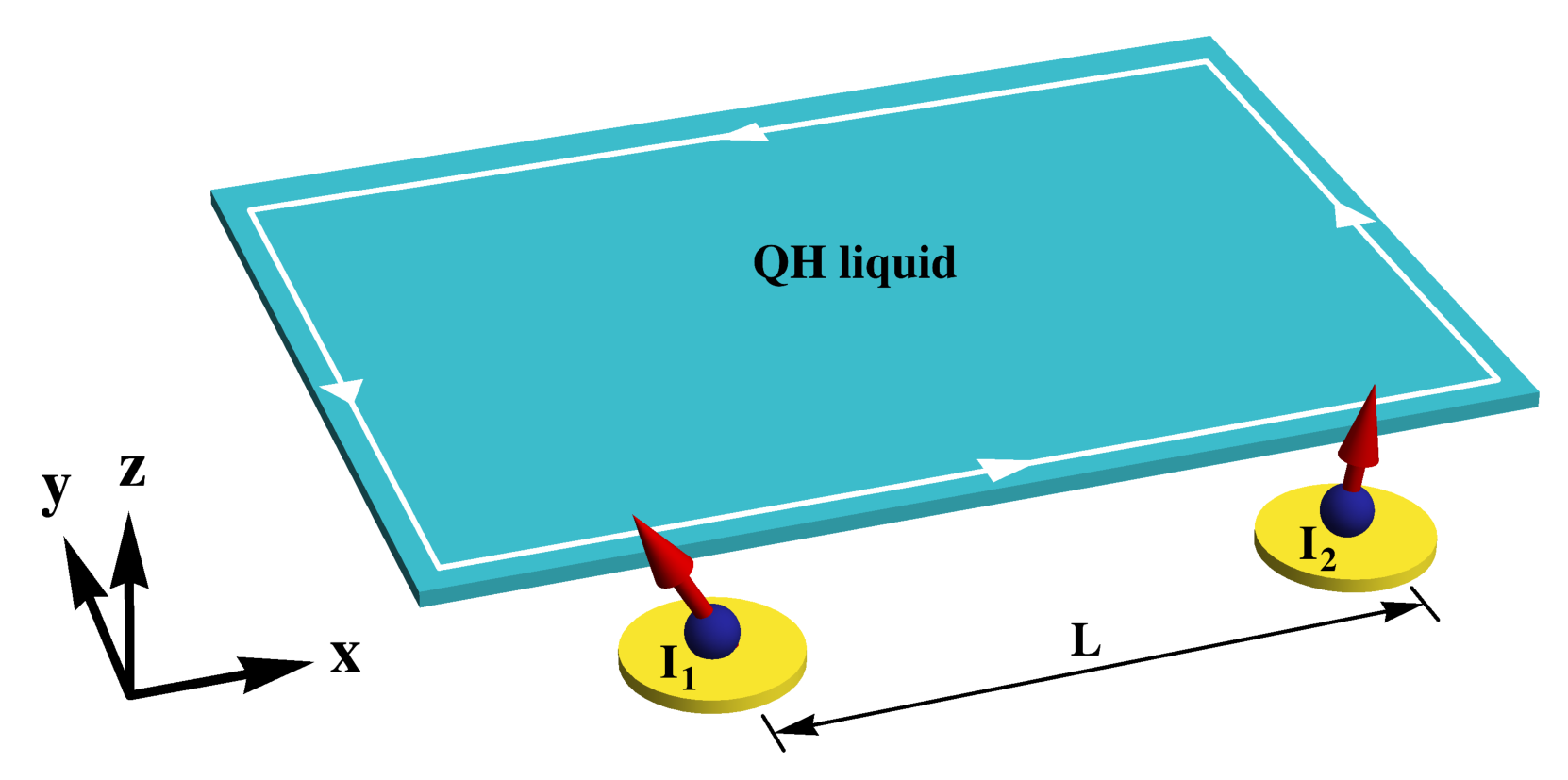
We now discuss the physics of RKKY interaction mediated by QH edge states. The basic setup is shown in Fig. 1. Two QDs are placed adjacent to a QH liquid, separated by a distance $L$ and labelled by the site index $i=1,2$. Conduction electrons in the QH edge state can tunnel into and out of the QDs [18] and thus can interact with the localized spins in them. This establishes coupling between the QH edge and the QDs. For simplicity, we treat the QDs as two spatial points. The Hamiltonian describing such a system has the form

where $H_{\textrm{edge}}$ is the Hamiltonian of conduction electrons in the edge state, $\mathbf{I}_{i}=(I_{i}^{x},I_{i}^{y},I_{i}^{z})$ denotes the localized spin in the $i$th QD, and $\mathbf{S}_{i}=(S_{i}^{x},S_{i}^{y},S_{i}^{z})$ denotes the spin of conduction electrons coupled to $\mathbf{I}_{i}$, with coupling strength $\Gamma_{i}$. Experimentally, $\Gamma_{i}$ can be tuned by gating. We define $\mathbf{S}_{i}$ to be the spin density in the edge state multiplied by the confinement length of the QDs. For the setup, we assume $L$ is large so that there is no direct interaction between the spins in the QDs.

In the weak tunnel coupling regime such that $\Gamma_{i}\ll E_{F}$, where $E_{F}$ is the Fermi energy of conduction electrons, the dynamics of the spins in the QDs effectively decouples from that of the conduction electrons. In such a case, one can derive an effective Hamiltonian for the spins in QDs, valid in the adiabatic regime, by performing a Schrieffer-Wolff transformation [20, 21] of Eq. (1) followed by tracing out the degrees of freedom of conduction electrons (see Appendix A for the derivation of effective Hamiltonian and a discussion of adiabaticity),

where the spin-component indices $\alpha,\beta=x,y,z$. The first term is the RKKY interaction, with $J_{ij}^{\alpha\beta}=\Gamma_{i}\Gamma_{j}\chi_{ij}^{\alpha\beta}/2$. Here $\chi_{ij}^{\alpha\beta}$ is the static spin susceptibility of conduction electrons, $\chi_{ij}^{\alpha\beta}=-i\int^{\infty}_{0}dt\ e^{-\eta t}\langle[S^{\alpha}_{i}(t),S^{\beta}_{j}(0)]\rangle$, where $\eta=0^{+}$ and $\langle\cdots\rangle$ denotes the average determined by $H_{\textrm{edge}}$. Physically, conduction electrons in the vicinity of a QD develop a spin-density oscillation due to their interaction with the spin in the QD. This spin-density response, determined by $\chi_{ij}^{\alpha\beta}$, can be perceived by the spins in other QDs coupled to the QH edge. In this way the RKKY interaction is established. For spin-unpolarized QH states, we assume $\langle S_{i}^{x}\rangle=\langle S_{i}^{y}\rangle=\langle S_{i}^{z}\rangle=0$, such that $\chi_{ij}^{\alpha\beta}=\delta^{\alpha\beta}\chi_{ij}^{\alpha\alpha}$. On the other hand, the in-plane spin operators $S_{i}^{x}$, $S_{i}^{y}$ are less relevant (in the renormalization group sense) than the out-of-plane ones $S_{i}^{z}$ in a QH state with full spin polarization, as we discuss below. In this case we set $S_{i}^{x}=S_{i}^{y}=0$ and hence $\chi_{ij}^{\alpha\beta}=\delta^{\alpha z}\delta^{\beta z}\chi_{ij}^{zz}$. Thus, in general we have $J_{ij}^{\alpha\beta}=\delta^{\alpha\beta}J_{ij}^{\alpha\alpha}$. The RKKY interaction leads to an effective exchange coupling $\mathcal{J}^{\alpha}=J^{\alpha\alpha}_{12}+J^{\alpha\alpha}_{21}$, as a function of the interdot distance $L$, between the localized spins $I^{\alpha}_{1}$ and $I^{\alpha}_{2}$. The effective onsite Zeeman fields $\mathbf{B}_{i}$ are a direct consequence of time-reversal (TR) symmetry breaking in QH systems. We find $\mathbf{B}_{i}=(\Gamma_{i}^{2}/2)\int_{0}^{\infty}dt\ e^{-\eta t}\langle\mathbf{S}_{i}(t)\times\mathbf{S}_{i}(0)\rangle$. In spin-polarized QH states, $\mathbf{B}_{i}=0$ (for more details and estimates we refer to Appendix A).

The RKKY interaction in Eq. (2) is by nature long-ranged and can be used as an approach to entangle spin qubits over long distances. Thus, it is important to understand how the interaction looks like in various QH systems. To this end, it is convenient to adopt a continuum description of the QH edge states that is well approximated by the chiral Luttinger liquid (LL) model at low energy [17]. In general, the edge of a QH liquid may support (electron-) density-fluctuation modes as well as Majorana fermions (zero-modes), with the action

written in the bosonization language [17] (throughout the article we set $\hbar=1$). The bosonic fields $\phi_{I}$ describe the density modes, and $\lambda_{K}$ denote the Majorana fermions. The symmetric matrix $K_{IJ}$ encodes the topological properties of the QH state, while the positive-definite symmetric matrix $V_{IJ}$ specifies the velocities and interactions of $\phi_{I}$. The parameter $v_{K}$ is the velocity of $\lambda_{K}$: $v_{K}>0$ ($v_{K}<0$) if the $\lambda_{K}$ is left-moving (right-moving).

Upon passing to the continuum limit, we replace the spin operators $S^{\alpha}_{i}(t)/l$ with spin density operators $S^{\alpha}(x_{i},t)$, where $l$ is the confinement length of the QDs and $x_{i}$ is the position of the $i$th QD. The nonvanishing components of the spin susceptibility are given by $\chi^{\alpha\alpha}_{ij}=-il^{2}\int^{\infty}_{0}dt\ e^{-\eta t}\langle[S^{\alpha}(x_{i},t),S^{\alpha}(x_{j},0)]\rangle$. Assuming translation invariance along the QH edge, which is justified for clean samples, we may further write $\chi^{\alpha\alpha}_{ij}=\chi^{\alpha\alpha}(x_{i}-x_{j})$, [22] where

with $\mathcal{T}$ the time-ordering operator. The correlators are evaluated in the zero-temperature limit. We define

where $\psi_{\sigma}=\sum_{\mu}\psi^{\mu}_{\sigma}$ is the sum of the most-relevant electron operators $\psi^{\mu}_{\sigma}$ with spin $\sigma=\uparrow,\downarrow$ on the QH edge.

The number of $\psi^{\mu}_{\uparrow}$ operators is not necessarily equal to that of $\psi^{\mu}_{\downarrow}$ operators since TR symmetry is broken. For instance, the most-relevant electron operators have the same spin in a spin-polarized QH state, so that $S^{x}=S^{y}=0$. This is in contrast to the situation in 1D systems where TR symmetry is present [23, 24]. Using bosonization, we express $S^{\alpha}$ in terms of the fields $\phi_{I}$ and $\lambda_{K}$, and compute the spin susceptibility.

We sketch the calculation of the spin susceptibility for a generic QH edge state (for particular examples, see Appendix B). First of all, we assume separation of charged and neutral degrees of freedom in the QH edge state. This phenomenon, as has been demonstrated experimentally in a number of QH systems [26, 25], results from strong Coulomb interaction among the elementary density modes $\phi_{I}$ and resembles “charge-spin separation” in a generic TR-invariant 1D system [22]. As a result, the physical modes that propagate on the QH edge are the charged and neutral collective modes as well as Majorana fermions. The physical parameters relevant to experiment are the velocities and interactions of these propagating modes, whose magnitudes are set by different energy scales in the QH system. For instance, the charged-mode velocity, determined by the dominant Coulomb energy scale, is much greater than the velocity of neutral mode and other parameters [25]. We make use of this fact in our calculation. For a moment, we consider the case of two density modes in the edge theory, see Eq. (3). To compute the correlators in Eq. (4), we define a new set of fields which diagonalize the action of the density modes $\phi_{I}$. The action takes the form

in the basis of new fields $\phi_{+}$ and $\phi_{-}$. Here $\varepsilon=1$ ($\varepsilon=-1$) if the edge states are chiral (non-chiral) and $v_{+},v_{-}>0$. New velocities $v_{+}$ and $v_{-}$ are well approximated by the velocities of the physical charged mode and neutral mode, respectively, so that $v_{+}\gg v_{-}$. Upon expressing the spin density operators in terms of the free fields $\phi_{+}$, $\phi_{-}$, and $\lambda_{K}$, it is straightforward to compute the correlators,

where $\delta>0$ is an infinitesimal and $\Delta k$ is the gauge-invariant momentum difference between the edge modes. The case $\Delta k=0$ corresponds to the scattering of an edge mode with itself. Here we have omitted the terms that are less relevant, and assumed $|v_{K}|=v_{-}$ as both of the velocities are determined by less dominant energy scales in the system. The exponents $g_{+}^{\alpha}$, $g_{-}^{\alpha}$ are functions of the matrices $K_{IJ}$ and $V_{IJ}$ and as we show $0<g_{+}^{\alpha}\ll 1$ and $g_{-}^{\alpha}>1$ (see Appendix B for the expressions in different QH states). Evaluating the time integral in Eq. (4), we obtain $\chi^{\alpha\alpha}(x)$, which in general may contain multiple terms for different momentum differences. We keep only the most-relevant terms.

The various QH states can be divided into three types: (i) Those with a chiral edge state containing a single density mode, such as the Laughlin states at filling factors $\nu=1/m$, where $m$ is an odd integer. (ii) Those with a chiral edge state containing multiple interacting density modes, such as the QH state at $\nu=2$. (iii) Those with a non-chiral edge state, such as the particle-hole dual states [27] of Laughlin states.

For QH states of type (i), we find $\chi^{\alpha\alpha}(x)=0$, taking into account the most-relevant spin operators in the edge state. Thus, to the lowest order the RKKY interaction cannot be established. Physically, the vanishing spin susceptibility reflects the homogeneous electronic structure in an independent QH edge mode, a property originating from the incompressibility of the QH liquid which prevents the formation of electronic spin texture. In reality, however, a small nonzero spin susceptibility may still be measured, due to higher-order processes involving virtual transitions to edge states in higher Landau levels.

In QH edge states of type (ii) and type (iii), the spin susceptibility is nonzero to the lowest order. In these cases, the inter-edge interactions introduce inhomogeneous degrees of freedom (“noise”) to the stream of conduction electrons, allowing for the development of spin-density oscillations. We find

for left-moving type (ii) edge states, where $g^{\alpha}=g_{+}^{\alpha}+g_{-}^{\alpha}-1$, $\Theta(x)$ is the Heaviside step function, and $C^{\alpha}(\boldsymbol{g}^{\alpha},\boldsymbol{v})$ are functions of $\boldsymbol{g}^{\alpha}=(g_{+}^{\alpha},g_{-}^{\alpha})$ and $\boldsymbol{v}=(v_{+},v_{-})$, whose explicit definitions are given in Appendix B. If the edge state is right-moving, one replaces $\Theta(-x)$ with $\Theta(x)$, and sends $\boldsymbol{v}\rightarrow-\boldsymbol{v}$ in $C^{\alpha}(\boldsymbol{g}^{\alpha},\boldsymbol{v})$. These findings suggest that the spin susceptibility in type (ii) edge states is “rectified”, i.e., directed in the down-stream direction of the propagation of conduction electrons, see Fig. 2(a), where left- and right-moving directions are defined with respect to the lower edge of the QH liquid (the same in Fig. 2(b)). This result is not surprising and can be understood also intuitively. In a left-moving edge state, conduction electrons move in the $-x$ direction, leading to the factor $\Theta(-x)$ in the expression of $\chi^{\alpha\alpha}(x)$. Formally, such an interesting form of the spin susceptibility is a manifestation of the causality principle in 1D chiral systems, where information is transported one-way and novel physical rules can emerge, e.g., see Ref. [28] for fluctuation-dissipation relations in chiral QH systems.

Lastly, we find

for type (iii) edge states, where $C^{\alpha}_{>}(\boldsymbol{g}^{\alpha},\boldsymbol{v})$ and $C^{\alpha}_{<}(\boldsymbol{g}^{\alpha},\boldsymbol{v})$ are functions of $\boldsymbol{g}^{\alpha}$ and $\boldsymbol{v}$, defined in Appendix B. The spin susceptibility in this case is “both-way”, as shown in Fig. 2(b), with different magnitudes in the $+x$ and $-x$ directions, i.e., $C^{\alpha}_{>}(\boldsymbol{g}^{\alpha},\boldsymbol{v})\neq C^{\alpha}_{<}(\boldsymbol{g}^{\alpha},\boldsymbol{v})$. This again reflects the inequivalence between left-moving and right-moving edge modes. Imagining now the chirality of all edge modes are reverted, e.g., by TR operation, the profile of the spin susceptibility should also be reverted. Indeed, we find that $C^{\alpha}_{>}(\boldsymbol{g}^{\alpha},\boldsymbol{v})$ are related to $C^{\alpha}_{<}(\boldsymbol{g}^{\alpha},\boldsymbol{v})$ by the exchange of arguments $v_{+}\leftrightarrow v_{-}$ and $g_{+}^{\alpha}\leftrightarrow g_{-}^{\alpha}$, which technically carries out the chirality-reverting procedure (see Appendix B). In the above discussion, we have assumed that spin excitations do not extend into the $L_{0}-L$ part of the QH edge, where $L_{0}$ is the total edge length. In practice, this is realized by grounding the $L_{0}-L$ part or by choosing the sample such that $L_{0}\gg L$.

The exponents $g^{\alpha}$, where $\alpha=x,y,z$, determine how the RKKY interaction scales with distance. In Table 1, we list them in different QH states. In general, $g^{\alpha}$ depend on both the chirality and spin polarization of the QH edge state. For chiral edge states, i.e., those of type (ii), these exponents are integral invariants depending on the topological order of the bulk liquid, whereas for non-chiral edge states they are nonuniversal and depend on the parameters in the Hamiltonian. In the latter case, we write $g^{\alpha}=g^{\alpha}_{0}+\delta g^{\alpha}$, where $g^{\alpha}_{0}$ is the integer part of $g^{\alpha}$. As shown in Appendix B, $\delta g^{\alpha}/g^{\alpha}_{0}\ll 1$ for all the non-chiral edge states in the table, assuming “charge-neutral separation” on the edge. Moreover, we find that the in-plane components of the RKKY interaction vanish in a spin-polarized QH state, leading to an Ising-type exchange coupling of spin qubits. On the other hand, the RKKY interaction has zero out-of-plane component and equal in-plane components in a spin-unpolarized QH state, which is XY-type. This suggests that a transformation of the anisotropy type of the RKKY interaction may be observed in the QH liquid at $\nu=2/3$, which was found to be spin-unpolarized at low fields and spin-polarized at high fields [29].

The QH state at $\nu=5/2$ is also of special interest. We consider both Abelian and non-Abelian topological orders proposed to describe this state. The former include the Halperin $331$ state [30] and 113 state [31], and the latter include the Moore-Read (Pfaffian) state [32], the anti-Pfaffian state [33, 34] and the $SU(2)_{2}$ state [35]. The $331$ state and $113$ state can be both spin-polarized and -unpolarized, just like the $\nu=2/3$ QH state. The Pfaffian state, like the Laughlin states, supports a single density mode on the edge and thus has vanishing RKKY interaction. The particle-hole dual state of the Pfaffian state, the anti-Pfaffian state, has a non-chiral edge state and a non-integer scaling exponent. For the $SU(2)_{2}$ state, we assume that the Majorana fermion and the neutral collective mode propagate at different velocities, as they should in reality, which is necessary to obtain a nonvanishing scaling exponent. Such careful treatment is not essential for other $\nu=5/2$ states. We have assumed that the RKKY interaction is mediated solely by the fractional edge modes in the second Landau level, while the integer edge modes in the lowest Landau level do not play a role. Experimentally, this can be fulfilled, using the fact that edge modes in different Landau levels are spatially separated [36]. For instance, the QDs in Fig. 1 can be moved out of the plane of the QH liquid and formed in a second two- or quasi-one-dimensional electron gas in the vertical direction [37, 38, 39, 40], such that they are in tunnel contact with the fractional edge modes but far away from the integer edge modes. The coupling between the integer edge and the QDs and the interaction between the integer edge and the fractional edge can be neglected to a good approximation.

Let us estimate the coupling between the two spin qubits in Fig. 1, given by $\mathcal{J}^{\alpha}=\Gamma_{1}\Gamma_{2}\{\chi^{\alpha\alpha}(L)+\chi^{\alpha\alpha}(-L)\}/2$. In Appendix B, we obtain the dimensional part $[\chi^{\alpha\alpha}(x)]$ of the spin susceptibility,

for both type (ii) and type (iii) edge states, where $a$ is the lattice constant of the underlying material hosting the QH system. For example, let us consider the QH state at $\nu=2$, realized in GaAs heterostructures. We have $a=0.565$ nm for GaAs, $g^{x}=g^{y}=1$, and $v_{-}\simeq 10^{4}$ m/s [25]. Using $\Gamma_{1}=\Gamma_{2}=\Gamma\simeq 0.1$ meV and $l=30$ nm (see Appendix C for the estimates), we find $\mathcal{J}^{x}=\mathcal{J}^{y}\simeq 1~\mu$eV for $L=1~\mu$m. This is about one order of magnitude smaller than the direct exchange strength $\mathcal{J}_{\textrm{direct}}\simeq 10-100~\mu$eV in typical GaAs double QDs [2] and is experimentally measurable. The RKKY interaction established by QH edge states thus provides a way to realize entangled quantum gates over mesoscopic distances. The implementation of two-qubit gates using Hamiltonians of the form of Eq. (2) is well known: see, e.g., Ref. [2] (footnote 13) for Ising-type coupling and Ref. [7] for XY-type coupling. The $\mu$eV exchange strength converts to gate-operation times of the order of nanoseconds, which is well below the coherence times [3] of spin qubits.

It is interesting to compare the RKKY interaction in QH edge states with that in semiconductor quantum wires. Assuming spin-rotation symmetry, the dimensional part $[\chi_{\textrm{w}}(x)]$ of the spin susceptibility in quantum wires can be found in Ref. [23]. The ratio

characterizes the relative strength of the RKKY interaction in the two sorts of systems, where $v_{F}$ is the Fermi velocity in the quantum wire and $g_{\textrm{w}}$ depends on the interaction of electrons. In non-interacting case, $g_{\textrm{w}}=1$. Consider the $\nu=2$ QH edge state and GaAs quantum wire. We find $r^{x}(L)=r^{y}(L)\simeq 1.5$ for $L=1~\mu$m, using $g_{\textrm{w}}=0.75$ and $v_{F}\simeq 10^{5}~$m/s [23]. In principle, quantum wires can also be used to mediated RKKY interaction between spin qubits. However, using QH edge states offers more advantages. From technical aspect, the edge states and the spin qubits can be realized in the same material, for instance, in a 2DEG in GaAs heterostructures, which is more experimentally accessible than a setup with quantum wires. More importantly, the topologically protected QH edge states are more immune to disorder effects and perturbations in the system than quantum wires. This guarantees a better quality of the long-distance quantum gates.

Our discussions so far have focused on the RKKY interaction between spin qubits. Interestingly, the treatments can also be applied to obtain the RKKY interaction between nuclear spins embedded in the 1D QH edge state (see also Ref. [41]). To this end, let $\Gamma_{i}\rightarrow A/N$ and $\mathbf{I}_{i}\rightarrow\tilde{\mathbf{I}}_{i}$ in Eq. (1) and the following equations, where $A$ is the hyperfine coupling constant, $N$ is the number of nuclear spins in a cross section (labelled by $i$) of the QH edge, and $\tilde{\mathbf{I}}_{i}$ is the total nuclear spin operator in a given cross section. Given a non-chiral edge state with both spin-up and spin-down electrons, e.g., the spin-unpolarized state at $\nu=2/3$, the nuclear spins may form a helical magnetic order [23] at low temperatures, induced by the RKKY interaction. The nuclear magnetic order acts back on the electronic system by gapping out conducting edge modes. Experimentally, such an order is evidenced by the reduction of the conductance at low temperatures [40].

By measuring the spatial dependence of RKKY interaction [19, 42], one can obtain information about the chirality and spin polarization of the QH edge state, which in turn are related to the topological order of the bulk QH liquid [17]. In particular, this technique may be used to detect the nature of the QH liquid at $\nu=5/2$: One can distinguish between a chiral edge state and a non-chiral edge state by confirming whether the spin susceptibility is unidirectional along the edge. One can rule out either a spin-polarized state or a spin-unpolarized state by comparing the in-plane and out-of-plane components of the RKKY interaction, by measuring the spin states in the QDs. For this one can make use of experimental techniques based on spin-to-charge conversion [2] developed for read-out of spin qubits in QDs [43, 44, 45]. The numerical values of the scaling exponents also help to identify the true $\nu=5/2$ state. The advantages of measuring the spin susceptibility are obvious, compared with other approaches detecting topological orders based on edge-bulk correspondence [17], such as measuring the temperature and voltage dependence of quasiparticle tunneling [46]. First, it is easier to vary the sampling point in space than in temperature or voltage, e.g., one may use the setup in Fig. 1 with an array of QDs. Second, information encoded in spin degrees of freedom is more robust than that encoded in charge current, against unfavorable modification due to long-range Coulomb interaction in the device [47]. Compared with electronic Fabry-Pérot [48, 49] and Mach-Zehnder [50, 51, 52] interferometries, our setup probes the non-Abelian topological orders at $\nu=5/2$ with a much simpler device geometry and more straightforward data.

The scenario becomes more complicated if one replaces the QDs with quantum anti-dots [53]. In that case, tunneling of quasiparticles, rather than electrons, defines the coupling between the QH edge and the anti-dots. It is still possible to define an RKKY interaction mediated by quasiparticles in the edge state, whose spatial dependence can be used to distinguish different Abelian QH states. For non-Abelian states, however, there are ambiguities in the scaling behavior of the RKKY interaction, arising from the multiple fusion channels of non-Abelian quasiparticles.

To conclude, we have introduced a novel approach to achieving long-distance entanglement of spin qubits confined in QDs, based on the RKKY interaction mediated by QH edge states. The approach allows for the implementation of quantum gates with long coupling ranges and fast operation times, which would greatly facilitate the development of large-scale quantum computers. From fundamental point of view, the ability to probe the chirality and the spin polarization of a QH edge state via measuring the spatial form of the RKKY interaction opens up a new venue for studying electronic and spin physics in QH systems.

References

- [1] M. A. Nielsen and I. L. Chuang, Quantum Computation and Quantum Information (Cambridge University Press, Cambridge, 2000).
- [2] D. Loss and D. DiVincenzo, Quantum Computation with Quantum Dots, Phys. Rev. A 57, 120 (1998).
- [3] C. Kloeffel and D. Loss, Prospects for Spin-Based Quantum Computing in Quantum Dots, Annu. Rev. Condens. Matter Phys. 4, 51 (2013).
- [4] H. Bluhm, S. Foletti, I. Neder, M. Rudner, D. Mahalu, V. Umansky, and A. Yacoby, Dephasing Time of GaAs Electron-Spin Qubits Coupled to a Nuclear Bath Exceeding s, Nature Phys. 7, 109 (2011).
- [5] K. M. Svore, B. M. Terhal, and D. P. DiVincenzo, Local Fault-Tolerant Quantum Computation, Phys. Rev. A 72, 022317 (2005).
- [6] A. M. Childs, H. L. Haselgrove, and M. A. Nielsen, Lower Bounds on the Complexity of Simulating Quantum Gates, Phys. Rev. A 68, 052311 (2003).
- [7] A. Imamog-lu, D. D. Awschalom, G. Burkard, D. P. DiVincenzo, D. Loss, M. Sherwin, and A. Small, Quantum Information Processing Using Quantum Dot Spins and Cavity QED, Phys. Rev. Lett. 83, 4204 (1999).
- [8] L. Childress, A. S. Sørensen, and M. D. Lukin, Mesoscopic Cavity Quantum Electrodynamics with Quantum Dots, Phys. Rev. A 69, 042302 (2004).
- [9] G. Burkard and A. Imamoglu, Ultra-Long-Distance Interaction between Spin Qubits, Phys. Rev. B 74, 041307(R) (2006).
- [10] M. Trif, V. N. Golovach, and D. Loss, Spin Dynamics in InAs Nanowire Quantum Dots Coupled to a Transmission Line, Phys. Rev. B 77, 045434 (2008).
- [11] L. Trifunovic, O. Dial, M. Trif, J. R. Wootton, R. Abebe, A. Yacoby, and D. Loss, Long-Distance Spin-Spin Coupling via Floating Gates, Phys. Rev. X 2, 011006 (2012).
- [12] L. Trifunovic, F. L. Pedrocchi, and D. Loss, Long-Distance Entanglement of Spin Qubits via Ferromagnet, Phys. Rev. X 3, 041023 (2013).
- [13] P. Stano, J. Klinovaja, F. R. Braakman, L. M. K. Vandersypen, and D. Loss, Fast Long-Distance Control of Spin Qubits by Photon-Assisted Cotunneling, Phys. Rev. B 92, 075302 (2015).
- [14] M. A. Ruderman and C. Kittel, Indirect Exchange Coupling of Nuclear Magnetic Moments by Conduction Electrons, Phys. Rev. 96, 99 (1954).
- [15] T. Kasuya, A Theory of Metallic Ferro- and Antiferromagnetism on Zener’s Model, Prog. Theor. Phys. 16, 45 (1956).
- [16] K. Yosida, Magnetic Properties of Cu-Mn Alloys, Phys. Rev. 106, 893 (1957).
- [17] X.-G. Wen, Quantum Field Theory of Many-Body Systems: From the Origin of Sound to an Origin of Light and Electrons (Oxford University Press, 2004).
- [18] H. Kiyama, T. Nakajima, S. Teraoka, A. Oiwa, and S. Tarucha, Spin-Dependent Current through a Quantum Dot from Spin-Polarized Nonequilibrium Quantum Hall Edge Channels, Phys. Rev. B 91, 155302 (2015).
- [19] P. Stano, J. Klinovaja, A. Yacoby, and D. Loss, Local Spin Susceptibilities of Low-Dimensional Electron Systems, Phys. Rev. B 88, 045441 (2013).
- [20] J. R. Schrieffer and P. A. Wolff, Relation between the Anderson and Kondo Hamiltonians, Phys. Rev. 149, 491 (1966).
- [21] S. Bravyi, D. P. DiVincenzo, and D. Loss, Schrieffer-Wolff Transformation for Quantum Many-Body Systems, Ann. Phys. (Amsterdam) 326, 2793 (2011).
- [22] T. Giamarchi, Quantum Physics in One Dimension (Oxford University Press, New York, 2003).
- [23] B. Braunecker, P. Simon, and D. Loss, Nuclear Magnetism and Electron Order in Interacting One-Dimensional Conductors, Phys. Rev. B , 165119 (2009).
- [24] Y.-W. Lee and Y.-L. Lee, Electrical Control and Interaction Effects of the RKKY Interaction in Helical Liquids, Phys. Rev. B , 214431 (2015).
- [25] E. Bocquillon, V. Freulon, J-.M Berroir, P. Degiovanni, B. Plaçais, A. Cavanna, Y. Jin, and G. Fève, Separation of Neutral and Charge modes in One-Dimensional Chiral Edge Channels, Nat. Commun. 4, 1839 (2013).
- [26] A. Bid, N. Ofek, H. Inoue, M. Heiblum, C. L. Kane, V. Umansky, and D. Mahalu, Observation of Neutral Modes in the Fractional Quantum Hall Regime, Nature (London) 466, 585 (2010).
- [27] S. M. Girvin, Particle-Hole Symmetry in the Anomalous Quantum Hall Effect, Phys. Rev. B 29, 6012(R) (1984).
- [28] C. Wang and D. E. Feldman, Chirality, Causality, and Fluctuation-Dissipation Theorems in Nonequilibrium Steady States, Phys. Rev. Lett. 110, 030602 (2013).
- [29] J. P. Eisenstein, H. L. Stormer, L. N. Pfeiffer, and K. W. West, Evidence for a Spin Transition in the Fractional Quantum Hall Effect, Phys. Rev. B 41, 7910(R) (1990).
- [30] B. I. Halperin, Theory of the Quantized Hall Conductance, Helv. Phys. Acta. 56, 75 (1983).
- [31] G. Yang and D. E. Feldman, Experimental Constraints and a Possible Quantum Hall State at , Phys. Rev. B 90, 161306(R) (2014).
- [32] G. Moore and N. Read, Nonabelions in the Fractional Quantum Hall Effect, Nucl. Phys. B 360, 362 (1991).
- [33] M. Levin, B. I. Halperin, and B. Rosenow, Particle-Hole Symmetry and the Pfaffian State, Phys. Rev. Lett. 99, 236806 (2007).
- [34] S.-S. Lee, S. Ryu, C. Nayak, and M. P. A. Fisher, Particle-Hole Symmetry and the Quantum Hall State, Phys. Rev. Lett. 99, 236807 (2007).
- [35] X.-G. Wen, Non-Abelian Statistics in the Fractional Quantum Hall States, Phys. Rev. Lett. 66, 802 (1991).
- [36] D. B. Chklovskii, B. I. Shklovskii, and L. I. Glazman, Electrostatics of Edge Channels, Phys. Rev. B 46, 4026 (1992).
- [37] J. P. Eisenstein, L. N. Pfeiffer, and K. W. West, Independently Contacted Two-Dimensional Electron Systems in Double Quantum Wells, Appl. Phys. Lett. 57, 2324 (1990).
- [38] O. M. Auslaender, A. Yacoby, R. de Picciotto, K. W. Baldwin, L. N. Pfeiffer, and K. W. West, Experimental Evidence for Resonant Tunneling in a Luttinger Liquid, Phys. Rev. Lett. 84, 1764 (2000).
- [39] L. Pfeiffer, H. L. Störmer, K. W. Baldwin, K. W. West, A. R. Goñi, A. Pinczuk, R. C. Ashoori, M. M. Dignam, W. Wegscheider, Cleaved Edge Overgrowth for Quantum Wire Fabrication, J. Cryst. Growth 127, 849 (1993).
- [40] C. P. Scheller, T.-M. Liu, G. Barak, A. Yacoby, L. N. Pfeiffer, K. W. West, and D. M. Zumbühl, Possible Evidence for Helical Nuclear Spin Order in GaAs Quantum Wires, Phys. Rev. Lett. 112, 066801 (2014).
- [41] T. Meng, P. Stano, J. Klinovaja, and D. Loss, Helical Nuclear Spin Order in a Strip of Stripes in the Quantum Hall Regime, Eur. Phys. J. B 87, 203 (2014).
- [42] L. Zhou, J. Wiebe, S. Lounis, E. Vedmedenko, F. Meier, S. Blügel, P. H. Dederichs, and R. Wiesendanger, Strength and Directionality of Surface Ruderman-Kittel-Kasuya-Yosida Interaction Mapped on the Atomic Scale, Nature Phys. 6, 187 (2010).
- [43] J. R. Petta, A. C. Johnson, J. M. Taylor, E. A. Laird, A. Yacoby, M. D. Lukin, C. M. Marcus, M. P. Hanson, and A. C. Gossard, Coherent Manipulation of Coupled Electron Spins in Semiconductor Quantum Dots, Science 309, 2180 (2005).
- [44] R. Hanson, L. P. Kouwenhoven, J. R. Petta, S. Tarucha, and L. M. K. Vandersypen, Spins in Few-Electron Quantum Dots, Rev. Mod. Phys. 79, 1217 (2007).
- [45] C. Barthel, D. J. Reilly, C. M. Marcus, M. P. Hanson, and A. C. Gossard, Rapid Single-Shot Measurement of a Singlet-Triplet Qubit, Phys. Rev. Lett. 103, 160503 (2009).
- [46] X.-G. Wen, Edge Transport Properties of the Fractional Quantum Hall States and Weak-Impurity Scattering of a One-Dimensional Charge-Density Wave, Phys. Rev. B 44, 5708 (1991).
- [47] G. Yang and D. E. Feldman, Influence of Device Geometry on Tunneling in the Quantum Hall Liquid, Phys. Rev. B 88, 085317 (2013).
- [48] A. Stern and B. I. Halperin, Proposed Experiments to Probe the Non-Abelian Quantum Hall State, Phys. Rev. Lett. 96, 016802 (2006).
- [49] P. Bonderson, A. Kitaev, and K. Shtengel, Detecting Non-Abelian Statistics in the Fractional Quantum Hall State, Phys. Rev. Lett. 96, 016803 (2006).
- [50] D. E. Feldman and A. Kitaev, Detecting Non-Abelian Statistics with an Electronic Mach-Zehnder Interferometer, Phys. Rev. Lett. 97, 186803 (2006).
- [51] C. Wang and D. E. Feldman, Identification of 331 Quantum Hall States with Mach-Zehnder Interferometry, Phys. Rev. B 82, 165314 (2010).
- [52] G. Yang, Probing the Quantum Hall State with Electronic Mach-Zehnder Interferometry, Phys. Rev. B 91, 115109 (2015).
- [53] M. R. Geller and D. Loss, Aharonov-Bohm Effect in the Chiral Luttinger Liquid, Phys. Rev. B 56, 9692 (1997).
- [54] D. Stepanenko, M. Rudner, B. I. Halperin, and D. Loss, Singlet-Triplet Splitting in Double Quantum Dots Due to Spin-Orbit and Hyperfine Interactions, Phys. Rev. B 85, 075416 (2012).