跳到论文正文
W Papers独立论文阅读器 arXiv:1509.08949 论文正文 计算阅读时间 · 0%
引用这篇论文根据当前论文元数据生成,正式投稿前建议核对。


License: arXiv.org perpetual non-exclusive license
arXiv:1509.08949v1 [hep-th] 29 Sep 2015

Generalized uncertainty principle and thermostatistics: a semiclassical approach

Mohammad Abbasiyan-Motlaq Affiliation: Department of Physics, Science and Research Branch, Islamic Azad University, Tehran, Iran    Pouria Pedram Electronic address: p.pedram@srbiau.ac.ir Affiliation: Department of Physics, Science and Research Branch, Islamic Azad University, Tehran, Iran
August 24, 2026
Abstract

We present an exact treatment of the thermodynamics of physical systems in the framework of the generalized uncertainty principle (GUP). Our purpose is to study and compare the consequences of two GUPs that one implies a minimal length while the other predicts a minimal length and a maximal momentum. Using a semiclassical method, we exactly calculate the modified internal energies and heat capacities in the presence of generalized commutation relations. We show that the total shift in these quantities only depends on the deformed algebra not on the system under study. Finally, the modified internal energy for an specific physical system such as ideal gas is obtained in the framework of two different GUPs.

Keywords: 
Generalized uncertainty principle, Thermostatistics, Minimal length, Maximal momentum.
pacs
04.06.Bc, 05.30.-d

I Introduction

As a significant consequence of various candidates of quantum gravity such as string theory, loop quantum gravity, doubly special relativity and black hole physics, the existence of a minimal observable length and/or a maximal observable momentum is suggested in the literature [1, 2, 3]. This minimal length is of the order of the Planck length ℓP=G​ℏ/c3≈10−35​m\ell_{\mathrm{P}}=\sqrt{{G\hbar}/{c^{3}}}\approx 10^{-35}m, where GG is Newton’s gravitational constant.

Based on these theories, the Heisenberg uncertainty principle is modified to the so-called Generalized (Gravitational) Uncertainty Principle (GUP) [4, 5]. Due to this modification, the Hamiltonian of the physical systems will be modified which results in the deformation of the physical properties of these systems in both quantum mechanical and classical levels. In the context of the GUP framework, various problems such as harmonic oscillator, hydrogen atom, gravitational quantum well, Casimir effect, Landau levels, Lamb’s shift, and particles scattering have been investigated exactly or approximately in Refs. [6, 7, 8, 9, 10, 11, 12, 13, 14].

In the context of the statistical mechanics, Fityo developed a semiclassical method for partition function evaluation based on modification of elementary cells of phase space according to deformed commutation relations and investigated the thermodynamical properties of some physical systems up to the first order of the GUP parameter [15]. Moreover, using exact solutions of the generalized Schrödinger equation [16, 17, 9, 18, 19], the effects of the minimal length on partition function, internal energy, and heat capacity in classical and quantum mechanical domains have been studied numerically in Refs. [9, 19, 20, 21, 22].

In this paper, we investigate the thermodynamical properties of the physical systems in the context of the generalized uncertainty principle. By using the results of Ref. [15], we obtained general relations that exactly calculate the modified internal energies and heat capacities in the presence of deformed commutation relations. Using exact solutions, we show that the total shift in internal energies and heat capacities does not depend on the physical systems and indeed it is related to the deformed algebra. We have also compared the results of our calculations in two different GUP frameworks. Finally, we obtain the modified internal energy for the ideal gas in these GUP frameworks.

II The Generalized Uncertainty Principle

First consider the following GUP in agreement with various theories of quantum gravity [23, 24, 25, 26, 27, 28] which is proposed by Kempf, Mangano and Mann (KMM) in one dimension [29, 16, 30, 31, 32, 33, 34]

Δ​X​Δ​P≥ℏ2​(1+β​(Δ​P)2+β​⟨P⟩2),\Delta X\Delta P\geq\frac{\hbar}{2}(1+\beta(\Delta P)^{2}+\beta\langle P\rangle^{2}), (1)

where β=β0/(c2​MPl2)\beta=\beta_{0}/(c^{2}M^{2}_{{\mathrm{Pl}}}) is the GUP parameter, MPl=ℏ​c/GM_{{\mathrm{Pl}}}=\sqrt{\hbar c/G} is the Planck mass and β0\beta_{0} is a dimensionless parameter of the order of unity. The relation (1) implies a minimal observable length proportional to the Planck length (Δ​X)m​i​n=ℏ​β=β0​ℓPl(\Delta X)_{min}=\hbar\sqrt{\beta}=\sqrt{\beta_{0}}\ell_{\mathrm{Pl}}. The above generalized uncertainty relation leads to modification of the canonical communication relations. In three-dimensions we have [29, 16, 30]

[Xi,Pj]=i​ℏ​((1+β​P2)​δi​j+β′​Pi​Pj),[Pi,Pj]=0,[Xi,Xj]=i​ℏ​2​β−β′+(2​β+β′)​β​P21+β​P2​(Pi​Xj−Pj​Xi),\begin{array}[]{l}[X_{i},P_{j}]=i\hbar\left((1+\beta P^{2})\delta_{ij}+\beta^{\prime}P_{i}P_{j}\right),\\ \left[P_{i},P_{j}\right]=0,\\ \left[X_{i},X_{j}\right]=i\hbar\dfrac{2\beta-\beta^{\prime}+(2\beta+\beta^{\prime})\beta P^{2}}{1+\beta P^{2}}(P_{i}X_{j}-P_{j}X_{i}),\end{array} (2)

where i,j=1,2,3i,j=1,2,3 and β,β′\beta,\beta^{\prime} are the GUP parameters. For this case, the minimal length becomes (Δ​X)m​i​n=ℏ​β+β′(\Delta X)_{min}=\hbar\sqrt{\beta+\beta^{\prime}}.

To incorporate the idea of maximal observable momentum in agreement with doubly special relativity theories, we use the recently proposed generalized uncertainty principle (GUP∗) which implies both the minimal length uncertainty and maximal observable momentum [31, 32]

[Xi,Pj]=i​ℏ​δi​j1−β​P2,[Pi,Pj]=0,[Xi,Xj]=2​i​ℏ​β(1−β​P2)2​(Pi​Xj−Pj​Xi),\displaystyle\begin{array}[]{l}\left[X_{i},P_{j}\right]=\dfrac{i\hbar\delta_{ij}}{1-\beta P^{2}},\\ \left[P_{i},P_{j}\right]=0,\\ \left[X_{i},X_{j}\right]=\dfrac{2i\hbar\beta}{(1-\beta P^{2})^{2}}(P_{i}X_{j}-P_{j}X_{i}),\end{array}

where (Δ​X)m​i​n=3​34​ℏ​β(\Delta X)_{min}=\frac{3\sqrt{3}}{4}\hbar\sqrt{\beta} and the momentum of the particle cannot exceed 1/β{1}/{\sqrt{\beta}}, i.e., Pm​a​x=1/βP_{max}={1}/{\sqrt{\beta}}. Note that, these generalized commutation relations are the particular forms of the general relations [35]

[Xi,Pj]=i​ℏ​fi​j​(β,β′,P),[Pi,Pj]=i​ℏ​hi​j​(β,β′,P),[Xi,Xj]=i​ℏ​gi​j​(β,β′,P).\displaystyle\begin{array}[]{l}\left[X_{i},P_{j}\right]=i\hbar\,f_{ij}(\beta,\beta^{\prime},P),\\ \left[P_{i},P_{j}\right]=i\hbar\,h_{ij}(\beta,\beta^{\prime},P),\\ \left[X_{i},X_{j}\right]=i\hbar\,g_{ij}(\beta,\beta^{\prime},P).\end{array}

Here, {β,β′}\{\beta,\beta^{\prime}\} are the GUP parameters and {fi​j,gi​j,hi​j}\{f_{ij},g_{ij},h_{ij}\} are deformation functions. In the limit β,β′→0\beta,\beta^{\prime}\rightarrow 0, fi​jf_{ij} goes to unity while gi​jg_{ij} and hi​jh_{ij} go to zero. Thus, the position and momentum operators tend to the ordinary position and momentum operators xix_{i} and pip_{i} satisfying [xi,pj]=i​ℏ​δi​j[x_{i},p_{j}]=i\hbar\delta_{ij}. In the classical limit ℏ→0\hbar\rightarrow 0 the quantum commutation relations lead to the Poisson brackets as

1i​ℏ​[A,B]⇒{A,B}.\dfrac{1}{i\hbar}[A,B]\Rightarrow\{A,B\}. (11)

The effects of the GUP on classical and quantum mechanical systems are addressed in Refs. [1, 17, 36, 37, 38, 39, 35, 40].

III GUP and the modified thermodynamics

The partition function for a system with NN non-interacting particles in the GUP framework is [15]

ZN=1h3​N​∫d3​N​X​d3​N​PJ​exp⁡[−H⁡(X,P)kB​T],Z_{N}=\dfrac{1}{h^{3N}}\int\dfrac{\mathrm{d}^{3N}X\mathrm{d}^{3N}P}{J}\exp\left[-\dfrac{H(X,P)}{k_{B}T}\right], (12)

where H⁡(X,P)H(X,P) is the Hamiltonian of the system, kBk_{B} is Boltzman’s constant, TT is the temperature, and J=∂(X1,P1,…,XD,PD)∂(x1,p1,…,xD,pD)J=\frac{\partial(X_{1},P_{1},\dots,X_{D},P_{D})}{\partial(x_{1},p_{1},\dots,x_{D},p_{D})} is the Jacobian of the transformation in DD-dimensions. Indeed, the Jacobian can be read off from the modified poisson brackets. In three-dimensions we have [15]

∂(X1,P1,X2,P2,X3,P3)∂(x1,p1,x2,p2,x3,p3)={X1,P1}​{X2,P2}​{X3,P3}−{X1,P3}​{P1,P2}​{X2,X3}−\displaystyle\frac{\partial(X_{1},P_{1},X_{2},P_{2},X_{3},P_{3})}{\partial(x_{1},p_{1},x_{2},p_{2},x_{3},p_{3})}=\left\{X_{1},P_{1}\right\}\left\{X_{2},P_{2}\right\}\left\{X_{3},P_{3}\right\}-\left\{X_{1},P_{3}\right\}\left\{P_{1},P_{2}\right\}\left\{X_{2},X_{3}\right\}-
{X1,P2}​{X2,P1}​{X3,P3}−{X1,P3}​{X2,P2}​{X3,P1}−{X1,P1}​{X2,P3}​{X3,P2}+\displaystyle\left\{X_{1},P_{2}\right\}\left\{X_{2},P_{1}\right\}\left\{X_{3},P_{3}\right\}-\left\{X_{1},P_{3}\right\}\left\{X_{2},P_{2}\right\}\left\{X_{3},P_{1}\right\}-\left\{X_{1},P_{1}\right\}\left\{X_{2},P_{3}\right\}\left\{X_{3},P_{2}\right\}+
{X1,X2}​{P1,P3}​{X3,P2}+{X1,P3}​{X2,P1}​{X3,P2}−{X1,X2}​{P2,P3}​{X3,P1}+\displaystyle\left\{X_{1},X_{2}\right\}\left\{P_{1},P_{3}\right\}\left\{X_{3},P_{2}\right\}+\left\{X_{1},P_{3}\right\}\left\{X_{2},P_{1}\right\}\left\{X_{3},P_{2}\right\}-\left\{X_{1},X_{2}\right\}\left\{P_{2},P_{3}\right\}\left\{X_{3},P_{1}\right\}+
{X1,P2}​{X2,X3}​{P1,P3}−{X1,X3}​{P1,P3}​{X2,P2}+{X1,X3}​{X2,P1}​{P2,P3}+\displaystyle\left\{X_{1},P_{2}\right\}\left\{X_{2},X_{3}\right\}\left\{P_{1},P_{3}\right\}-\left\{X_{1},X_{3}\right\}\left\{P_{1},P_{3}\right\}\left\{X_{2},P_{2}\right\}+\left\{X_{1},X_{3}\right\}\left\{X_{2},P_{1}\right\}\left\{P_{2},P_{3}\right\}+
{X1,X3}​{P1,P2}​{X2,P3}−{X1,X2}​{P1,P2}​{X3,P3}−{X1,P1}​{X2,X3}​{P2,P3}+\displaystyle\left\{X_{1},X_{3}\right\}\left\{P_{1},P_{2}\right\}\left\{X_{2},P_{3}\right\}-\left\{X_{1},X_{2}\right\}\left\{P_{1},P_{2}\right\}\left\{X_{3},P_{3}\right\}-\left\{X_{1},P_{1}\right\}\left\{X_{2},X_{3}\right\}\left\{P_{2},P_{3}\right\}+
{X1,P2}​{X2,P3}​{X3,P1}.\displaystyle\left\{X_{1},P_{2}\right\}\left\{X_{2},P_{3}\right\}\left\{X_{3},P_{1}\right\}. (13)

For the deformed commutation relations (II), the Hamiltonian can be written in the following form

H=P22​m+U⁡(X),H=\dfrac{P^{2}}{2m}+U(X), (14)

and the relation (12) becomes

ZN=1h3​N​∫d3​N​X​exp⁡[−U⁡(X)kB​T]​∫d3​N​P​exp⁡[−P22​m​kB​T]J⁡(β,β′,P),Z_{N}=\dfrac{1}{h^{3N}}\displaystyle{\int\mathrm{d}^{3N}X\exp\Big[-\dfrac{U(X)}{k_{B}T}\Big]}\displaystyle{\int\mathrm{d}^{3N}P\dfrac{\exp\Big[-\dfrac{P^{2}}{2mk_{B}T}\Big]}{J(\beta,\beta^{\prime},P)}}, (15)

where U⁡(X)U(X) is the potential function. In ordinary thermodynamics we have

ZN0=1h3​N​∫d3​N​x​d3​N​p​exp⁡[−H0​(x,p)kB​T],Z^{0}_{N}=\dfrac{1}{h^{3N}}\displaystyle{\int\mathrm{d}^{3N}x\,\mathrm{d}^{3N}p\,\exp\Big[-\dfrac{H_{0}(x,p)}{k_{B}T}\Big]}, (16)

where H0=p2/2​m+U⁡(x)H_{0}={p^{2}}/{2m}+U(x) is the Hamiltonian for the non-deformed case. Now, since

∫d3​N​x​exp⁡[−U⁡(x)kB​T]=ℏ3​N​ZN0​(2​π​m​kB​T)−32​N,{\int\mathrm{d}^{3N}x\,\exp\Big[-\dfrac{U(x)}{k_{B}T}\Big]}=\hbar^{3N}Z_{N}^{0}\left(2\pi mk_{B}T\right)^{-\frac{3}{2}N}, (17)

we obtain

ZN=ZN0​(2​π​m​kB​T)−32​N​∫d3​N​P​exp⁡[−P22​m​kB​T]J⁡(β,β′,P).Z_{N}=Z^{0}_{N}\left(2\pi mk_{B}T\right)^{-\frac{3}{2}N}\displaystyle{\int\mathrm{d}^{3N}P\dfrac{\exp\Big[-\dfrac{P^{2}}{2mk_{B}T}\Big]}{J(\beta,\beta^{\prime},P)}}. (18)

Thus, the modified internal energy E=−∂∂(kB​T)​ln⁡ZE=-\frac{\partial}{\partial(k_{B}T)}\ln Z and heat capacity C=∂E∂TC=\frac{\partial E}{\partial T}, are given by

E=E0−32​N​kB​T+N2​m​S2S0,C=C0−32​N​kB−N4​m2​kB​T2​S4​S0−(S2)2(S0)2,\begin{array}[]{l}E=E^{0}-\dfrac{3}{2}Nk_{B}T+\dfrac{N}{2m}\dfrac{S_{2}}{S_{0}},\\ C=C^{0}-\dfrac{3}{2}Nk_{B}-\dfrac{N}{4m^{2}k_{B}T^{2}}\dfrac{S_{4}S_{0}-(S_{2})^{2}}{(S_{0})^{2}},\end{array} (19)

where Sn=∫d3​P​Pn​exp⁡[−P22​m​kB​T]J⁡(β,β′,P)S_{n}=\displaystyle{\int\mathrm{d}^{3}P\,P^{n}\dfrac{\exp\Big[-\dfrac{P^{2}}{2mk_{B}T}\Big]}{J(\beta,\beta^{\prime},P)}}. Here, E0E^{0} and C0C^{0} are the internal energy and the heat capacity in ordinary thermodynamics, respectively, i.e., E0=−∂∂(kB​T)​ln⁡Z0E^{0}=-\frac{\partial}{\partial(k_{B}T)}\ln Z^{0} and C0=∂E0∂TC^{0}=\frac{\partial E^{0}}{\partial T}. After integrating out the angular parts, the above equations can be written as

E=E0−32​N​kB​T+N2​m​s4s2,C=C0−32​N​kB−N4​m2​kB​T2​s6​s2−(s4)2(s2)2,\begin{array}[]{l}E=E^{0}-\dfrac{3}{2}Nk_{B}T+\dfrac{N}{2m}\dfrac{s_{4}}{s_{2}},\\ C=C^{0}-\dfrac{3}{2}Nk_{B}-\dfrac{N}{4m^{2}k_{B}T^{2}}\dfrac{s_{6}s_{2}-(s_{4})^{2}}{(s_{2})^{2}},\end{array} (20)

where sn=∫d​P​Pn​exp⁡[−P22​m​kB​T]J⁡(β,β′,P)s_{n}=\displaystyle{\int\mathrm{d}P\,P^{n}\dfrac{\exp\Big[-\dfrac{P^{2}}{2mk_{B}T}\Big]}{J(\beta,\beta^{\prime},P)}}. Other modified thermodynamical quantities such as Helmholtz free energy A=−kB​T​ln⁡ZA=-k_{B}T\ln Z and entropy S=kB​ln⁡Z+E/TS=k_{B}\ln Z+{E}/{T} can be obtained in a similar manner.

IV Applications

In the following subsections, we investigate the effects of two GUPs (2,II) on the thermodynamical properties of the physical systems. The KMM’s GUP framework implies a minimal length while the high order GUP framework (GUP∗) predicts minimal length and maximal momentum. We also compare the results for both GUPs.

IV.1 KMM’s GUP: minimal length

In three-dimensional space, the KMM’s GUP is given by Eq. (2). For this case, the Jacobian of the transformation reads [15]

J=(1+β​P2)2​(1+(β+β′)​P2).J=(1+\beta P^{2})^{2}(1+(\beta+\beta^{\prime})P^{2}). (21)

So, using Eq. (20) we obtain the following exact relation for the internal energy

E=E0−32​N​kB​T+N2​m​β​−Ω1​Γ​(12,12​β​ξ)+β​(Ω2+Ω3​Γ​(12,12​(β+β′)​ξ))Ω4​Γ​(12,12​β​ξ)+Ω5−Ω6​Γ​(12,12​(β+β′)​ξ),E=E^{0}-\dfrac{3}{2}Nk_{B}T+\dfrac{N}{2m\beta}\dfrac{-\Omega_{1}\Gamma\Big(\dfrac{1}{2},\dfrac{1}{2\beta\xi}\Big)+\sqrt{\beta}\bigg(\Omega_{2}+\Omega_{3}\Gamma\Big(\dfrac{1}{2},\dfrac{1}{2(\beta+\beta^{\prime})\xi}\Big)\bigg)}{\Omega_{4}\Gamma\Big(\dfrac{1}{2},\dfrac{1}{2\beta\xi}\Big)+\Omega_{5}-\Omega_{6}\Gamma\Big(\dfrac{1}{2},\dfrac{1}{2(\beta+\beta^{\prime})\xi}\Big)}, (22)

where ξ=m​kB​T\xi=mk_{B}T and

{Ω1=β′+β​(−β′−β′​β​ξ+2​β2​ξ)​exp⁡(12​β​ξ),Ω2=−β′​2​(β′+β)​ξ,Ω3=2​β2​ξ​exp⁡(12​(β+β′)​ξ),Ω4=β′+β​(−β′+β′​β​ξ+2​β2​ξ)​exp⁡(12​β​ξ),Ω5=β′​2​β​(β′+β)​ξ,Ω6=2​β​(β+β′)​β​exp⁡(12​(β+β′)​ξ).\displaystyle\left\{\begin{array}[]{l}\Omega_{1}=\sqrt{\beta^{\prime}+\beta}\Big(-\beta^{\prime}-\beta^{\prime}\beta\xi+2\beta^{2}\xi\Big)\exp\left({\frac{1}{2\beta\xi}}\right),\\ \Omega_{2}=-\beta^{\prime}\sqrt{2(\beta^{\prime}+\beta)\xi},\\ \Omega_{3}=2\beta^{2}\xi\exp\left({\frac{1}{2(\beta+\beta^{\prime})\xi}}\right),\\ \Omega_{4}=\sqrt{\beta^{\prime}+\beta}\Big(-\beta^{\prime}+\beta^{\prime}\beta\xi+2\beta^{2}\xi\Big)\exp\left({\frac{1}{2\beta\xi}}\right),\\ \Omega_{5}=\beta^{\prime}\sqrt{2\beta(\beta^{\prime}+\beta)\xi},\\ \Omega_{6}=2\beta(\beta+\beta^{\prime})\sqrt{\beta}\,\exp\left({\frac{1}{2(\beta+\beta^{\prime})\xi}}\right).\end{array}\right.

The exact heat capacity is given by

C=\displaystyle C= C0−32​N​kB+12​N​kBm​T​(β′)2\displaystyle C^{0}-\dfrac{3}{2}Nk_{B}+\dfrac{1}{2}N\sqrt{\dfrac{k_{B}}{mT}}(\beta^{\prime})^{2} (30)
×Ψ1​Γ​(12,(12​β​ξ)2)+Ψ2−Ψ3​Γ​(12,12​(β+β′)​ξ)+Ψ4+Ψ5​Γ​(12,12​(β+β′)​ξ)β⁡(β+β′)​[Ψ6​Γ​(12,12​ξ)+ξ​β​[Ψ7−Ψ8​Γ​(12,12​(β+β′)​ξ)]]2,\displaystyle\times\dfrac{\Psi_{1}\Gamma\Big(\dfrac{1}{2},\big(\dfrac{1}{2\beta\xi}\big)^{2}\Big)+\Psi_{2}-\Psi_{3}\Gamma\Big(\dfrac{1}{2},\dfrac{1}{2(\beta+\beta^{\prime})\xi}\Big)+\Psi_{4}+\Psi_{5}\Gamma\Big(\dfrac{1}{2},\dfrac{1}{2(\beta+\beta^{\prime})\xi}\Big)}{\sqrt{\beta(\beta+\beta^{\prime})}\bigg[\Psi_{6}\Gamma\Big(\dfrac{1}{2},\dfrac{1}{2\xi}\Big)+\xi\sqrt{\beta}\Big[\Psi_{7}-\Psi_{8}\Gamma\Big(\dfrac{1}{2},\dfrac{1}{2(\beta+\beta^{\prime})\xi}\Big)\Big]\bigg]^{2}},

in which

{Ψ1=−2​(β+β′)32​π​β​ξ​exp⁡(1β​ξ),Ψ2=2​β′​β⁡(β+β′)​ξ,Ψ3=2​β​(β′+2​β​β′​ξ+2​β2​ξ)​exp⁡(12​(β+β′)​ξ),Ψ4=2​(β+β′)​(−β′+β​β′​ξ+2​β2​ξ)​exp⁡(12​β​ξ)​Γ​(12,12​β​ξ),Ψ5=1ξ(β′+3ββ′ξ+2β2ξ)exp(β′+2​β2​β​(β+β′)​ξ)Γ((12,12​β​ξ),Ψ6=β+β′​(−β′+β​β′​ξ+2​β2​ξ)​exp⁡(12​β​ξ),Ψ7=β′​2​(β+β′)ξ,Ψ8=2​β​(β+β′)​exp⁡(12​(β+β′)​ξ),\displaystyle\left\{\begin{array}[]{l}\Psi_{1}=-2\big(\beta+\beta^{\prime}\big)^{\frac{3}{2}}\sqrt{\pi\beta\xi}\,\exp\left({\frac{1}{\beta\xi}}\right),\\ \Psi_{2}=2\beta^{\prime}\sqrt{\beta(\beta+\beta^{\prime})\xi},\\ \Psi_{3}=\sqrt{2\beta}\Big(\beta^{\prime}+2\beta\beta^{\prime}\xi+2\beta^{2}\xi\Big)\exp\left({\frac{1}{2(\beta+\beta^{\prime})\xi}}\right),\\ \Psi_{4}=\sqrt{2(\beta+\beta^{\prime})}\Big(-\beta^{\prime}+\beta\beta^{\prime}\xi+2\beta^{2}\xi\Big)\exp\left({\frac{1}{2\beta\xi}}\right)\Gamma\left(\dfrac{1}{2},\dfrac{1}{2\beta\xi}\right),\\ \Psi_{5}=\sqrt{\dfrac{1}{\xi}}\Big(\beta^{\prime}+3\beta\beta^{\prime}\xi+2\beta^{2}\xi\Big)\exp\left({\frac{\beta^{\prime}+2\beta}{2\beta(\beta+\beta^{\prime})\xi}}\right)\Gamma\left((\dfrac{1}{2},\dfrac{1}{2\beta\xi}\right),\\ \Psi_{6}=\sqrt{\beta+\beta^{\prime}}\Big(-\beta^{\prime}+\beta\beta^{\prime}\xi+2\beta^{2}\xi\Big)\exp\left({\frac{1}{2\beta\xi}}\right),\\ \Psi_{7}=\beta^{\prime}\sqrt{\dfrac{2(\beta+\beta^{\prime})}{\xi}},\\ \Psi_{8}=2\beta\Big(\beta+\beta^{\prime}\Big)\exp\left({\frac{1}{2(\beta+\beta^{\prime})\xi}}\right),\end{array}\right.

and Γ⁡(a,x)=∫x∞ta−1​e−t​𝑑t\Gamma(a,x)=\int_{x}^{\infty}t^{a-1}e^{-t}\mathrm{d}t is the incomplete gamma function. In the limit β,β′⟶0\beta,\beta^{\prime}\longrightarrow 0, the internal energy and heat capacity tend to E0E^{0} and C0C^{0}, respectively, as it is expected.

Notice that, although the changes in the energies and heat capacities depend on the modified algebra, these changes are similar for all physical systems. It is worth mentioning that the effects of GUP on various physical systems are also addressed in Refs. [6, 7, 8, 10, 11, 12, 13, 14]. In particular, the effects of minimal length on thermostatistics of classical and quantum mechanical systems have been studied in Refs. [19, 20, 21, 22].

IV.2 GUP∗: minimal length and maximal momentum

For GUP∗ the Jacobian of transformation becomes

J=1(1−β​P2)3,J=\dfrac{1}{(1-\beta P^{2})^{3}}, (40)

Now, using Eq. (20) we obtain the exact internal energy as

E=E0−32​N​kB​T+N2​m​Θ1​exp⁡(−12​β​ξ)−Θ2​Γ​(12,12​β​ξ)Θ3​exp⁡(−12​β​ξ)+Θ4​Γ​(12,12​β​ξ),\displaystyle E=E^{0}-\frac{3}{2}Nk_{B}T+\frac{N}{2m}\frac{\Theta_{1}\exp\left(\dfrac{-1}{2\beta\xi}\right)-\Theta_{2}\Gamma\left(\dfrac{1}{2},\dfrac{1}{2\beta\xi}\right)}{\Theta_{3}\exp\left(\dfrac{-1}{2\beta\xi}\right)+\Theta_{4}\Gamma\left(\dfrac{1}{2},\dfrac{1}{2\beta\xi}\right)}, (41)

where

{Θ1=3​β​ξ​T2​(1−315​β2​ξ​T),Θ2=32​T32​(−β​ξ+15​β2​ξ2−105​β3​ξ3+315​β4​ξ4),Θ3=β​ξ​T​(1−10​β​ξ+105​β2​ξ2),Θ4=12​ξ​T12​(1−9​β​ξ+45​β2​ξ2−105​β3​ξ3).\displaystyle\left\{\begin{array}[]{l}\Theta_{1}=3\sqrt{\beta}\xi T^{2}\Big(1-315\beta^{2}\xi T\Big),\\ \Theta_{2}=\frac{3}{\sqrt{2}}T^{\frac{3}{2}}\Big(-\beta\xi+15\beta^{2}\xi^{2}-105\beta^{3}\xi^{3}+315\beta^{4}\xi^{4}\Big),\\ \Theta_{3}=\sqrt{\beta}\xi T\Big(1-10\beta\xi+105\beta^{2}\xi^{2}\Big),\\ \Theta_{4}=\frac{1}{\sqrt{2}}\xi T^{\frac{1}{2}}\Big(1-9\beta\xi+45\beta^{2}\xi^{2}-105\beta^{3}\xi^{3}\Big).\end{array}\right.

For the heat capacity, we exactly find

C\displaystyle C =\displaystyle= C0−32​N​kB+3​N​kB\displaystyle C^{0}-\dfrac{3}{2}Nk_{B}+3Nk_{B} (47)
×Δ1−2​Δ2​exp⁡(12​β​ξ)​Γ​(12,12​β​ξ)+π​Δ3​exp⁡(1β​ξ)​Γ​(12,(12​β​ξ)2)[Δ4+Δ5​exp⁡(12​β​ξ)​Γ​(12,12​β​ξ)]2,\displaystyle\times\dfrac{\Delta_{1}-2\Delta_{2}\exp\left(\dfrac{1}{2\beta\xi}\right)\Gamma\left(\dfrac{1}{2},\dfrac{1}{2\beta\xi}\right)+\sqrt{\pi}\Delta_{3}\exp\left(\dfrac{1}{\beta\xi}\right)\Gamma\left(\dfrac{1}{2},\Big(\dfrac{1}{2\beta\xi}\Big)^{2}\right)}{\left[\Delta_{4}+\Delta_{5}\exp\left(\dfrac{1}{2\beta\xi}\right)\Gamma\left(\dfrac{1}{2},\dfrac{1}{2\beta\xi}\right)\right]^{2}},

where

{Δ1=18​β​ξ+210​T​(8​β3​ξ2−60​β4​ξ3+315​β5​ξ4),Δ2=2​β​ξ​(−5+11​β​ξ−630​β2​ξ2+4410​β3​ξ3−17325​β4​ξ4+33075​β5​ξ5),Δ3=1−30​β​ξ+405​β2​ξ2−2940​β3​ξ3+11655​β4​ξ4−28350​β5​ξ5+33075​β6​ξ6,Δ4=β​ξ​(−2+20​β​ξ−210​β2​ξ2),Δ5=2​(−1+9​β​ξ−45​β2​ξ2+105​β3​ξ3).\displaystyle\left\{\begin{array}[]{l}\Delta_{1}=18\beta\xi+210T\Big(8\beta^{3}\xi^{2}-60\beta^{4}\xi^{3}+315\beta^{5}\xi^{4}\Big),\\ \Delta_{2}=\sqrt{2\beta\xi}\Big(-5+11\beta\xi-630\beta^{2}\xi^{2}+4410\beta^{3}\xi^{3}-17325\beta^{4}\xi^{4}+33075\beta^{5}\xi^{5}\Big),\\ \Delta_{3}=1-30\beta\xi+405\beta^{2}\xi^{2}-2940\beta^{3}\xi^{3}+11655\beta^{4}\xi^{4}-28350\beta^{5}\xi^{5}+33075\beta^{6}\xi^{6},\\ \Delta_{4}=\sqrt{\beta\xi}\Big(-2+20\beta\xi-210\beta^{2}\xi^{2}\Big),\\ \Delta_{5}=\sqrt{2}\Big(-1+9\beta\xi-45\beta^{2}\xi^{2}+105\beta^{3}\xi^{3}\Big).\end{array}\right.
Refer to caption
Figure 1: The shift of internal energy (E−E0)/N{(E-E^{0})}/{N} versus TT for KMM’s GUP (blue line) and GUP∗ (red line). We set m=kB=1m=k_{B}=1 and β=β′=0.1\beta=\beta^{\prime}=0.1.

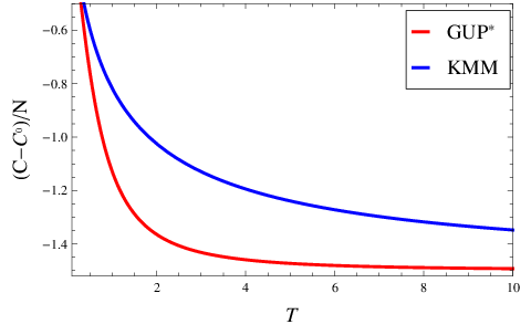
It is worth mentioning that the shift in the internal energies and heat capacities for physical systems does not depend on the type of the system. For comparison, we plotted (E−E0)/N{(E-E^{0})}/{N} (see Fig. 1) and (C−C0)/N{(C-C^{0})}/{N} (see Fig. 2) in terms of temperature in KMM’s GUP and GUP∗ frameworks. As it can be seen from Fig. 1, the energy shift of physical systems for GUP∗ is greater than the KMM’s GUP. Fig. 2 shows the similar result for the heat capacity. Moreover, in the high temperature limit, the heat capacity tends to zero for both cases, namely C⁡(T→∞)=0C(T\rightarrow\infty)=0 in agreement with Ref. [15]. Thus, according to the relation C=∂E∂TC=\frac{\partial E}{\partial T}, the internal energy asymptotically tends to a maximum value.
Refer to caption
Figure 2: The shift of heat capacity (C−C0)/N{(C-C^{0})}/{N} versus TT for KMM’s GUP (blue line) and GUP∗ (red line). We set m=kB=1m=k_{B}=1 and β=β′=0.1\beta=\beta^{\prime}=0.1.

Finally, we have shown the internal energy versus temperature for the ideal gas system in Fig. 3. As this figure shows, in low temperature limit, the behavior of ideal gas’s internal energy for both the KMM’s GUP and GUP∗ coincides. However, in high temperature limit, the internal energy of the ideal gas in the KMM’s GUP is greater than the internal energy in the GUP∗ framework and contains a maximum value in both scenarios. The exact maximum value of internal energy for the ideal gas in the KMM’s GUP is given by

Em​a​xK​M​M=1+2​ββ′+β2​m​β,\displaystyle E_{max}^{KMM}=\dfrac{1+\dfrac{2\sqrt{\beta}}{\sqrt{\beta^{\prime}+\beta}}}{2m\beta}, (54)

It is worthwhile to note that in the GUP∗ framework the momentum of particle can not exceed 1/β{1}/{\sqrt{\beta}}. Therefore, we expect that the temperature of the system represent a maximum value. At this temperature the heat capacity of systems is zero. Using Eq. (20) we obtain the following relation to calculate the value of maximum temperature for the ideal gas system

s6​s2−(s4)2=0,\displaystyle s_{6}s_{2}-(s_{4})^{2}=0, (55)

which can be solved numerically. At high temperature limit, i.e., 2​m​kB​T≫12mk_{B}T\gg 1, we have

Tm​a​x≈730​m​kB​β.\displaystyle T_{max}\approx\dfrac{7}{30mk_{B}\beta}. (56)

At this temperature, Em​a​xE_{max} for the ideal gas becomes

Em​a​xG​U​P∗\displaystyle E_{max}^{GUP^{*}} =\displaystyle= 63​(24010+1400​m​kB−157​105​π​e157​(m​kB)32​E​r​f​[157])20​m3​kB2​β​(55230+29​e157​105​π​m​kB​E​r​f​[157]).\displaystyle\dfrac{63\Big(24010+1400mk_{B}-157\sqrt{105\pi}e^{\frac{15}{7}}(mk_{B})^{\frac{3}{2}}Erf[\sqrt{\frac{15}{7}}]\Big)}{20m^{3}k^{2}_{B}\beta\Big(55230+29e^{\frac{15}{7}}\sqrt{105\pi mk_{B}}Erf[\sqrt{\frac{15}{7}}]\Big)}. (57)

For instance, for m=kB=1m=k_{B}=1 and β=β′=0.1\beta=\beta^{\prime}=0.1 these maximum values are found to be 12.07 and 1.07 for the KMM’s GUP and GUP∗, respectively. Also, the internal energy and heat capacity of other physical systems such as harmonic oscillator can be calculated by substituting the value of E0E_{0} and C0C_{0} in Eq. (20). Furthermore, the modified partition function Eq. (18) up to the first order of GUP parameter in KMM’s GUP framework [15] and GUP∗, are respectively given by

ZK​M​M\displaystyle Z^{KMM} =\displaystyle= Z0​(1−3​(3​β+β′)​m​kB​T+⋯),\displaystyle Z_{0}\Big(1-3(3\beta+\beta^{\prime})mk_{B}T+\cdot\cdot\cdot\Big), (58)
ZG​U​P∗\displaystyle Z^{GUP^{*}} =\displaystyle= Z0​(1−9​β​m​kB​T+⋯).\displaystyle Z_{0}\Big(1-9\beta mk_{B}T+\cdot\cdot\cdot\Big). (59)

In fact, for β′=0\beta^{\prime}=0, Eqs. (58) and (59) become identical. This is an expected result, due to equality of two GUP frameworks to the first order of GUP parameter when β′=0\beta^{\prime}=0.

Refer to caption
Figure 3: The internal energy of ideal gas E/N{E}/{N} versus TT for KMM’s GUP (blue line) and GUP∗ (red line). We set m=kB=1m=k_{B}=1 and β=β′=0.1\beta=\beta^{\prime}=0.1.

V Conclusions

In this paper, we have studied the thermodynamics of physical systems in the framework of the generalized uncertainty principle [1, 2, 3, 19, 20, 21, 22]. We obtained exact semiclassical relations in order to calculate the internal energy and heat capacity of physical systems in a general deformed algebra. We showed that the shift in internal energies and heat capacities are the same for all physical systems and only depends on the chosen deformed algebra. We applied this method for GUP∗ and KMM’s GUP and obtained the GUP-corrected thermodynamical variables. Furthermore, we investigated the behavior of internal energy for the ideal gas system in these frameworks. It is shown that for small temperature limit, the behavior of the internal energy is the same for both cases. However, in high temperature limit, the internal energy monotonically increases versus temperature such that EKMM>EGUP∗E_{\mathrm{KMM}}>E_{\mathrm{GUP^{*}}}.

References

  • [1] S. Hossenfelder, Living Rev. Relativity 16, 2 (2013).
  • [2] E. Witten, Phys. Today 49, 24 (1996).
  • [3] C.A. Mead, Phys. Rev. B 135, 849 (1964).
  • [4] M. Maggiore, Phys. Lett. B 319, 207 (1993).
  • [5] M. Maggiore, Phys. Rev. D 49, 5182 (1994).
  • [6] S. Das, E.C. Vagenas, Can. J. Phys. 87, 233 (2009).
  • [7] C. Quesne, V.M. Tkachuk, J. Phys. A 36, 10373 (2003).
  • [8] F. Brau, J. Phys. A 32, 7691 (1999).
  • [9] P. Pedram, Phys. Rev. D 85, 024016 (2012).
  • [10] S. Mignemi, Phys. Rev. D 84, 025021 (2011).
  • [11] Kh. Nouricer. J. Phys. A 38, 10027 (2005).
  • [12] F. Brau, F. Buisseret, Phys. Rev. D 74, 036002 (2006).
  • [13] U. Harbach, S. Hossenfelder, Phys. Lett. B 632, 379 (2006).
  • [14] M.M. Stetsko, V.M. Takachuk, Phys. Rev. A 76, 012707 (2007).
  • [15] T.V. Fityo, Phys. Lett. A 372, 5872 (2008).
  • [16] A. Kempf, G. Mangano and R.B. Mann, Phys. Rev. D 52, 1108 (1995).
  • [17] L.N. Chang, D. Minic, N. Okamura and T. Takeuchi, Phys. Rev. D 65, 125027 (2002).
  • [18] K. Nozari, T. Azizi, Int. J. Quant. Inf. 3, 623 (2005).
  • [19] K. Nozari, P. Pedram, Eur. Phys. Lett. 92, 50013 (2010).
  • [20] S.K. Rama, Phys. Lett. B 519, 903 (2001).
  • [21] B. Vakili, M.A. Gorji, J. Stat. Mech. P10013 (2012).
  • [22] M. Abbasiyan-Motlaq, P. Pedram, J. Stat. Mech. 497281 (2014).
  • [23] D. Amati, M. Ciafaloni and G. Veneziano, Phys. Lett. B 216, 41 (1989).
  • [24] D.J. Gross, P.F. Mende, Nucl. Phys. B 303, 407 (1988).
  • [25] L.J. Garay, Int. J. Mod. Phys. A 10, 145 (1995).
  • [26] M. Maggiore, Phys. Lett. B 304, 65 (1993).
  • [27] M. Kato, Phys. Lett. B 245, 43 (1990).
  • [28] F. Scardigli, Phys. Lett. B 452, 39 (1999).
  • [29] A. Kempf, J. Math. Phys. 35, 4483 (1994).
  • [30] A. Kempf, J. Phys. A 30, 2093 (1997).
  • [31] P. Pedram, Phys. Lett. B 714, 317 (2012).
  • [32] P. Pedram, Phys. Lett. B 718, 638 (2012).
  • [33] S. Das, E.C. Vagenas, Phys. Rev. Lett. 101, 221301 (2008).
  • [34] A.F. Ali, S. Das, E.C.Vagenas, Phys. Rev. D 84, 044013 (2011).
  • [35] S. Hossenfelder, Phys. Rev. D 73, 105013 (2006).
  • [36] C. Quesne, V.M. Tkachuk, J. Phys. A 37, 10095 (2004).
  • [37] C. Quesne, V.M. Tkachuk, J. Phys. A 38, 1747 (2005).
  • [38] P. Pedram, Adv. High Energy Phys. 2013, 853696 (2013).
  • [39] M.M. Stetsko, V.M. Takachuk, Phys. Rev. A 74, 012101 (2006).
  • [40] M.M. Stetsko, Phys. Rev. A 74, 062105 (2006).