Gibbs flow for approximate transport with applications to Bayesian computation
Abstract
Let and be two distributions on the Borel space . Any measurable function such that if is called a transport map from to . For any and , if one could obtain an analytical expression for a transport map from to , then this could be straightforwardly applied to sample from any distribution. One would map draws from an easy-to-sample distribution to the target distribution using this transport map. Although it is usually impossible to obtain an explicit transport map for complex target distributions, we show here how to build a tractable approximation of a novel transport map. This is achieved by moving samples from using an ordinary differential equation with a velocity field that depends on the full conditional distributions of the target. Even when this ordinary differential equation is time-discretized and the full conditional distributions are numerically approximated, the resulting distribution of mapped samples can be efficiently evaluated and used as a proposal within sequential Monte Carlo samplers. We demonstrate significant gains over state-of-the-art sequential Monte Carlo samplers at a fixed computational complexity on a variety of applications.
Keywords: Mass transport; Markov chain Monte Carlo; Normalizing constants; Path Sampling; Sequential Monte Carlo.
1 Introduction
The use of the Bayesian formalism of inference is ubiquitous in many areas of science. For statistical models of practical interest, implementation usually relies on Monte Carlo methods to sample from the posterior distribution which might be high dimensional and exhibit complex dependencies. Most available Monte Carlo algorithms rely on proposal distributions and the efficiency of these techniques is crucially dependent on whether these proposals are able to capture important features of the target. In this paper, we leverage ideas from the mass transport literature to develop a new methodology to build efficient proposal distributions which can be used within sequential Monte Carlo (SMC) samplers [39, 11, 19].
Given initial and target distributions and defined on , which in a Bayesian context may be interpreted as the prior and posterior, a transport map is a measurable function such that if . The transport map terminology arises from the fact that one can view as transporting the probability mass represented by to the probability mass represented by . We will use the notation since is the push-forward measure of by . Characterizing the existence of transport maps has generated a large literature in mathematics; see [55] for a recent review. In particular, much work has been dedicated to the Monge-Kantorovich problem, where one seeks the optimal transport map minimizing the expected cost .
For the purposes of Monte Carlo simulation, any analytically tractable transport map would allow us to map samples from to . However, even without imposing any optimality condition, such transport maps have only been identified in simple scenarios; e.g. when both and are Gaussian [44, Remark 2.30]. To obtain an approximate transport map, [35, 21, 42] proposed to minimize some measure of discrepancy between and , over a set of maps parametrized by a finite-dimensional parameter , e.g. a linear combination of some basis functions. However, it can be difficult to identify an appropriate subspace of candidate maps, and the resulting optimization problem is generally non-convex unless stringent assumptions are made [30, 43] and high dimensional in the absence of conditional independence structure in the target [49]. In this article, we circumvent these difficulties by considering a different approach to build approximate transport maps.
The transport maps we will consider are derived from a fluid dynamics interpretation of mass transport. Consider a curve of distributions connecting to ; e.g. the geometric path where is an increasing smooth function satisfying and . The use of bridging distributions between distant and is at the core of many state-of-the-art Monte Carlo methods such as path sampling [24, 41] and annealed importance sampling [15, 29, 39, 11]. If we view probability mass as an infinite ensemble of fluid particles, the main idea is to move these particles deterministically, using an ordinary differential equation (ODE) with a carefully designed velocity field, so as to mimic the time evolution of over the time interval . Loosely speaking, we may think of the movement of particles under such a velocity field as implicitly defining flow transport maps satisfying for each .
The idea of constructing transport maps using flows originates from [38]; see also [26, 16, 4] for other early contributions. This approach has since been adopted in a range of application domains ranging from engineering to physics [3, 14, 18, 50, 53]. Noting that, for a given curve of distributions, there could be multiple velocity fields achieving the flow transport, various optimality criteria have been introduced to identify a unique solution [38, 45, 50]; e.g. [45] proposed seeking the velocity field minimizing kinetic energy. In these contributions, the optimal velocity field is given by the solution of an elliptic partial differential equation (PDE). However, when using a full grid, PDE solvers suffer from the curse of dimensionality [17, 40] which could render them impractical. Sparse grid methods may be capable of dealing with sufficiently high dimensions but they come with their own set of approximations, e.g. tensor approximations [10, 17]. Using techniques from differential geometry, [6] constructed a flow transport using contact Hamiltonian flows that also determines adaptively, but the velocity field depends on intractable integrals on which would have to be numerically approximated.
An alternative approach involves building analytically tractable approximations of intractable flow transport maps. For example, in a Bayesian filtering context where is a Gaussian prior distribution on unknown states , and the likelihood is also Gaussian distributed with mean vector and a known covariance matrix, [8] proposed linearizing locally to exploit analytical tractability of Gaussian flows [5, 46, 48]. This article also proposes approximate flow transport maps that are analytically tractable, but the details of our construction are markedly different. Our approach does not require any distributional assumptions on and , instead it is based on approximating a novel flow that takes reference to the conditional distributions , , …, and the marginal distribution where for . As these distributions are typically intractable, we propose a tractable approximation which moves particles using a velocity field designed to track the full conditional distributions , where and . We shall refer to the latter as the Gibbs flow in reference to the Gibbs sampler. Contrary to existing transport-based methods, Gibbs flow does not require selecting a parametric class of maps, solving a non-convex optimization problem, approximating the solution of a PDE or approximating -dimensional integrals. Analogous to Gibbs samplers, its implementation allows one to leverage any conditional independence structure in the target and analytical tractability of any full conditional distribution to move the corresponding component. For components with intractable Gibbs flow, we will show that by further blocking these components into one-dimensional components, the resulting Gibbs velocity field only involves one-dimensional integrals w.r.t. the corresponding full conditional distributions that can be efficiently approximated using most quadrature routines. We will also introduce a novel time discretization scheme reminiscent of the systematic scan Gibbs sampler to numerically integrate the Gibbs flow. Although other numerical integrators can also be considered, our scheme allows efficient computation of the distribution of resulting mapped samples in high dimensions, which is crucial when employing such distributions as proposals within SMC samplers. Our approach only requires a computational cost of at each time step without requiring additional approximations to reduce the computational complexity [27]. We establish various theoretical properties of the Gibbs flow and demonstrate significant gains over state-of-the-art methods at a fixed computational complexity on a variety of applications.
The rest of the paper is organized as follows. In Section 2, we introduce the construction of transport maps using flows in a Bayesian context. We present a novel flow transport, the Gibbs flow approximation and its properties in Section 3. We then discuss how the Gibbs flow can be numerically implemented and employed as proposal distributions within SMC samplers in Section 4. Lastly, in Section 5, we illustrate the proposed methodology on a mixture model, a variance component model, and a log-Gaussian Cox point process model. The proof of all results are given in the Appendix. An R package is available at github.com/jeremyhengjm/GibbsFlow to reproduce all numerical results.
2 Transport with flows
2.1 A curve from prior to posterior
Let be a prior distribution on the Borel space and denote a likelihood function. To simplify presentation, we shall assume that is absolutely continuous w.r.t. the Lebesgue measure on , with an everywhere positive density , and that is also positive everywhere and satisfies . We will defer a discussion of improper priors to Section 5.2 and suppress all notational dependencies on observations. From Bayes’ rule, the resulting posterior distribution admits the density
| (1) |
where denotes the marginal likelihood. Henceforth we shall additionally assume that , where denotes the set of functions from to which are -times continuously differentiable.
We introduce a curve of distributions smoothly bridging the prior to the posterior by gradually introducing the likelihood using a strictly increasing -function such that and :
| (2) |
where . The function is commonly known as inverse temperature in the context of simulated annealing for optimization problems [31]. By differentiating (2) w.r.t. the time variable , we obtain its time evolution along the curve
| (3) |
where denotes the time derivative of and
| (4) |
is assumed to be finite for all . Under our assumptions, the family of models is regular so interchanging the order of differentiation w.r.t. the time variable and integration w.r.t. the spatial variable in the last equality of (4) is valid. By integrating (4) on the time interval , we recover the well-known path sampling identity [24, 41]:
| (5) |
Equation (3) reveals that the expected log-likelihood plays the role of a reference value which controls the evolution of the density , i.e. in logarithmic scale, the local behaviour around a point is such that there is an increase or decrease in density if or , respectively. In the following, we will see that this difference, when integrated w.r.t. , provides us with the right direction to move particles at time . The factors and in (3) are also intuitive as the change in density must be proportional how quickly we introduce the likelihood and how much probability mass there is locally. It will be apparent later that these factors dictate the speed of particles. We note that the contact Hamiltonian flow proposed in [6] also depends on the term which the author therein approximates using Monte Carlo methods.
2.2 Particle dynamics, Liouville’s equation and flow transport problem
Consider a particle trajectory in , initialized at time with a random draw , and evolved deterministically according to the following ODE
| (6) |
with velocity field . Under appropriate regularity conditions on which will be detailed later, this ODE admits a unique solution for all . Therefore we can define the flow map as
| (7) |
which associates the initial position of the particle to its position at time . It can be shown that flow maps are -diffeomorphisms, i.e. for each , is invertible and both and its inverse are continuously differentiable. These properties render flow maps ideal candidates as transport maps.
Additionally, if we denote the marginal distribution of by , the curve of distributions satisfies, under regularity conditions, the Liouville PDE [22, eq. (3.5.13), p. 54] also known as the continuity equation [2, eq. (8.1.1), p. 169]:
| (8) |
for . Notationally, and denote the partial derivatives of w.r.t. and , respectively, and the divergence operator is defined as for any . The Liouville PDE can be seen as the Fokker–Planck equation in the case of zero diffusivity; an informal but intuitive derivation of this PDE is given in Appendix A.
We can now describe the flow transport problem as identifying a velocity field such that the curve of target distributions in (2) is the solution of Liouville equation (8), i.e. we seek a that satisfies
| (9) |
for . If such a velocity field is regular enough that the resulting ODE (6) admits a unique solution for all and initial positions , then this allows us to construct the flow maps (7) that satisfy for all . As a consequence, we can obtain samples from by taking . The following result presents sufficient conditions on velocity fields that satisfy (9) to ensure the validity of this approach.
Theorem 1.
Suppose is a velocity field that satisfies Liouville equation (9) and the following conditions:
- A1.
-
(continuously differentiable) ;
- A2.
-
(space-time integrability) .
Then for -almost everywhere , there exists a unique solution to the ODE (6) for all . Therefore the flow maps defined by (7) are flow transports, i.e. for all .
Theorem 1 is a summary of results in [2] written for our purposes; see Appendix B for more details. With Theorem 1 in place, we can now formally define the flow transport problem as identifying a velocity field that satisfies Liouville’s equation (9) and Assumptions A1-A2. Although these assumptions are only sufficient conditions, we stress that pathologies can occur when these regularity conditions do not hold. This is illustrated in Appendix G.3, where we exhibit a velocity field that solves (9) and prove that it yields divergent particle trajectories.
3 A novel flow transport and Gibbs flow approximation
As alluded to in the introduction, the flow transport problem is typically underdetermined. Although various optimality criteria could be employed to attain unicity, they lead to velocity fields that are implicitly defined by solutions of elliptic PDEs. In this section, we begin by presenting an explicit solution to the flow transport problem before introducing the Gibbs flow approximation.
3.1 A flow transport solution on
We first discuss the one-dimensional case before considering the multivariate case. In this case, there is a well-known solution to the flow transport problem; see e.g. [3]. We will also establish that this coincides with the minimal kinetic energy solution considered in [45, 46].
Proposition 1.
Define the velocity field as
| (10) |
and assume that there exists an such that as with a constant that is independent of . Then the velocity field (10) solves the flow transport problem on and is additionally the minimal kinetic energy solution, i.e. for each
| (11) |
where .
To build intuition, we can rewrite (10) using (3) as
| (12) |
where and is the cumulative distribution function (CDF) of . The velocity field (12) may be likened to driving a vehicle. The denominator corresponds to the accelerator, since, e.g., particles in the tails of need to speed up to meet the changing schedule of intermediate distributions. Also, it is intuitive that particle speeds are proportional to the rate at which we introduce the likelihood. The numerator amounts to the steering wheel: a particle’s direction of travel is given by the relative difference between its current location , described by the term , and where the particle needs to go, prescribed by the term which contains information from the likelihood.
3.2 A novel flow transport on ,
It is tempting to extend (10) to the multivariate case by simply introducing the velocity field given for by
| (13) |
where and the integrand of (13) is to be understood as . This velocity field was previously mentioned in [3] and it can be shown to satisfy Liouville’s equation (9) whenever . However, we show in Appendix G.3 that (13) does not solve the flow transport problem as an ODE with velocity field would yield divergent particle trajectories even on a simple Gaussian example. The main reason for this pathology is the tail behaviour of .
We now give our solution to the flow transport problem in the multivariate case which recovers Proposition 1 when . We will write and denote the marginal distribution of in the component by and its CDF by .
Proposition 2.
Our construction is a generalization of a method proposed by [7] to build a compactly supported three-dimensional velocity field solving a flow transport problem in the context of molecular quantum chemistry. When the target distributions factorize into independent one-dimensional components, i.e. , we establish in Appendix C that the velocity field in (14)-(15) would simply reduce to
| (16) |
which is the solution of the one-dimensional flow transport problem for each marginal distribution given by Proposition 1. As the integrals in (14)-(15) can be seen as expectations w.r.t. the conditional distributions , , …, and the marginal distribution , we see that the flow transport is achieved by taking reference to these conditionals. We refer the reader to Appendix G for an illustration of flow transport solutions when the curve of distributions (2) lies in the Gaussian family.
3.3 Gibbs flow approximation
Despite the explicit form of the flow transport solution in Proposition 2, evaluating the velocity field (14)-(15) would require computing integrals of dimension up to . For computational tractability, we propose an approximate flow transport that takes reference to the full conditional distributions , where and . For component , the time evolution of its full conditional distribution is given by
| (17) |
where . We will design Gibbs velocity fields that track changes in the full conditionals (17) by seeking solutions to the following coupled system of Liouville equations
| (18) |
for and . Note that the Liouville equation for each full conditional distribution in (18) is defined on , so the divergence operator only acts on the variables .
For one-dimensional components, i.e. the case , the velocity field
| (19) |
which only involves one-dimensional integrals, can be shown to satisfy (18) for the -component, using similar arguments as in Proposition 1. For components with dimension , one could exploit analytical tractability of full conditional distributions when they lie in the exponential family to determine Gibbs velocity fields, or further block these components into one-dimensional components and employ (19). We will illustrate how to systematically determine Gibbs velocity fields on specific applications in Section 5, and will assume for now that we have such a velocity field satisfying (18). The following result presents sufficient conditions on a Gibbs velocity field to ensure that, with initial position the ODE
| (20) |
admits a unique solution for all .
Proposition 3.
Suppose is a velocity field that satisfies the system of Liouville equations (18) and the following conditions:
- A3.
-
(continuously differentiable) ;
- A4.
-
(tail behaviour) there exists satisfying and such that for all and , where denotes the dot product.
Then for -almost everywhere , there exists a unique solution to the ODE (20) for all .
Assumption A3 imposes some regularity on the Gibbs velocity field and Assumption A4 requires existence of a Lyapunov function so that a particle has non-increasing values of if it lies in the tails. In some cases, one can choose as a Lyapunov function; we establish this in the case in Appendix D. Under the conclusions of Proposition 3, we can define the Gibbs flow map as for each . Since the system (18) is only a (tractable) approximation of the desired Liouville equation (9), the marginal distribution of under the Gibbs flow, , will in general not be equal to the target distribution . We now provide a characterization of this error in terms of the following time-dependent local error:
| (21) |
which measures how well the Gibbs velocity field mimics the desired change in density (3). The sum over all components in (21) reveals the nature of the Gibbs flow approximation: information about how much probability mass is changing in a particular component is not communicated to other components. In other words, computational tractability is gained at the expense of breaking down a global problem in dimensions to many lower dimensional problems. For any function , we will write if is -integrable, and if is bounded.
Proposition 4.
Suppose is a velocity field that satisfies the system of Liouville equations (18), Assumptions A3-A4 and
- A5.
-
(tail decay) there exists such that
as with constants that are independent of .
Then the Gibbs flow approximation error is characterized by the following inequality
| (22) |
for , where .
The upper bound (22) is tight in the sense that it is equal to zero when the target distributions have independent components, i.e. . When the latter is not the case, we observe that the bound deteriorates with time, which is to be expected as errors can accumulate. To mitigate accumulation of errors, we will combine Gibbs flow with Markov chain Monte Carlo moves in Section 4.3. Rewriting (21) using (3) and (17) reveals that the inverse temperature should be chosen such that its derivative is small at those time instances when the integrated local error is large, as this would reduce the magnitude of the resulting -error in (22). We refer the reader to [24, 41, 57] for other works on how to select . For simplicity, all simulations in Section 5 and the Appendix will employ a quadratic inverse temperature function, i.e. . Lastly, like with any Gibbs sampler, we expect the use of any appropriate model specific reparameterization to also reduce the -error in (22).
4 Gibbs flow samplers
4.1 Numerical implementation
Given a target distribution of interest, we advocate exploiting any analytical tractability of full conditional distributions to determine a Gibbs velocity field (e.g. Section 5.2). For components without such tractability, a generic strategy would be to further block these components into one-dimensional components and rely on (19). We first note that (19) can be computed solely using one-dimensional integrals as the intractable normalizing constant cancels in the expression:
| (23) |
and the CDF of can be rewritten as
| (24) |
The one-dimensional integrals in (23)-(24) are integrals of the form for some integrand and domain . Here we consider the class of composite Newton-Cotes quadrature rules
| (25) |
where are quadrature weights which depend on the degree of the approximation and are many equispaced quadrature points in [28, p. 34]. We take (25) to be of the closed type, i.e. and take the endpoints of 11 1 Unbounded domains are treated with suitable truncation., as this choice will be convenient for domains of the type for . The composite quadrature rule (25) is derived by integrating Lagrange interpolation polynomials on subintervals; the degree of which dictates the accuracy of the approximation on each subinterval. We shall denote the resulting approximation of by ; for components with analytically tractable Gibbs velocity field , we set .
We now consider how to approximate a particle trajectory driven by the ODE
| (26) |
with initial condition . We will introduce a novel numerical integration scheme that is reminiscent of the systematic Gibbs scan. In the following, we will show that our proposed scheme, in contrast to standard numerical integrators, allows efficient computation of marginal distributions in high dimensions. For simplicity, we discretize the time interval into a regular grid with a constant step size ; non-constant step sizes can also be employed. To evolve a particle with position at time on the subinterval , we consider
for the first component, with the other components fixed as . If the solution is analytically tractable, we set ; otherwise we will rely on the Euler discretization
| (27) |
Similarly, we update the second component by considering
| (28) |
with , and setting if the solution is available or
otherwise. We then iteratively update all other components in a systematic manner to obtain .
In summary, the above procedure defines the maps
(with and ) which update one component at a time. By iterating over all components, the composition
| (29) |
defines our numerical integration scheme. The flow maps induced by this scheme
| (30) |
can be shown to be a first order approximation of the flow maps defined by (26) (see Appendix E), i.e. for all if the step size is sufficiently small22 2 This error result holds even if Euler discretizations are employed for some or all components..
4.2 Distribution of approximate Gibbs flow samples
We now detail how to compute the marginal distributions of under the numerically approximated Gibbs flow (30). This allows us to utilize these distributions as proposal distributions within a sequential importance sampler.
Under the assumptions of Proposition 3, the Gibbs flow maps are -diffeomorphisms by construction. Hence their approximation (30) will be injective if the step size is sufficiently small and quadrature approximations (if employed) are accurate enough - see [8, 34] for similar arguments. Under these conditions, it follows from a change of variables that the density of , is
| (31) |
where is given by the inverse map, denotes the absolute value of the determinant of the Jacobian matrix of . In numerical implementations, monotonicity may be monitored by checking for any sign changes in the Jacobian determinant. From (30), the latter can be computed as
Using the structure of our numerical integration scheme (29), the computational cost of computing
is at most . This cost may be even lower in statistical models with conditional independence structure as Gibbs velocity fields will inherent such structures yielding sparse Jacobian matrices (e.g. Section 5.2).
In the case of (19) for one-dimensional components and the Euler discretization (27), computing
requires the partial derivative of the approximate Gibbs velocity field . It turns out that we can compute by simply replacing integrals in the partial derivative of the Gibbs velocity field
with approximations based on the same quadrature rule. This follows from the following argument which allows one to compute the partial derivative w.r.t. of approximations of integrals of the form . Denote by the underlying Lagrange interpolant giving rise to the quadrature rule (25). By the first fundamental theorem of calculus and the closed property of (25)
| (32) |
To illustrate the computational savings our proposed numerical integrator (29) offers over standard integrators like the forward Euler method
| (33) |
we consider the case of solely one-dimensional components, i.e. for all . In the absence of any sparsity, computing the Jacobian determinant of the mapping in (33) would cost at most ; in contrast the cost associated to (29) is only .
Given independent samples from (30), the above discussion allows us to employ the marginal distribution in (31) as a proposal distribution within an importance sampling approximation of . The importance weights can be computed recursively using
with . An algorithmic description of the resulting sequential importance sampler is detailed in Algorithm 1. Using the output, we can approximate expectations of the form with the weighted sum , and estimate the marginal likelihood unbiasedly with . The adequacy of the importance sampling approximation based on the Gibbs flow can be monitored using the effective sample size (ESS) introduced in [32]. This quantity takes values between and , and will be equal to if samples are distributed according to the target distribution.
Input: prior , likelihood , inverse temperature , step size , and Gibbs velocity field .
For time step
For
(a) sample ;
(b) set and ;
(c) set and .
For time step
For
For
(d) set using Section 4.1;
(e) compute using Section 4.2;
(f) set and ;
(g) compute unnormalized weights
(h) compute normalized weights ;
(i) compute effective sample size ;
(j) compute normalizing constant estimator .
Output: samples , normalized weights and normalizing constant estimator .
4.3 Combining Gibbs flow with Markov chain Monte Carlo
State-of-the-art methods based on annealed importance sampling (AIS) simulate inhomogeneous Markov chains and for and , where is a -invariant Markov chain Monte Carlo (MCMC) kernel. For each , although the marginal distribution of is typically intractable, one can still use these samples within an importance sampling approximation of , by associating sample with the importance weight
| (34) |
with and . The choice of bridging distributions and MCMC kernels can have a large impact on algorithmic performance; if these kernels mix slowly and/or the intermediate distributions are too distant, the variance of the importance weights (34) can be very high.
To improve the performance of AIS, references [53, 54] suggested adding deterministic maps which attempt to “push” samples from to , but the authors did not propose a generic methodology to construct such transport maps. In our context, we will rely on numerical approximation of the Gibbs flow, as described in Section 4.1, to build these maps. Practically, for , we initialize by sampling and setting . For , we then iterate by setting , as defined in (29), and sampling from a -invariant MCMC kernel. Like in AIS, we can also use the samples within an importance sampling approximation of . The importance weights are given by
for with . We provide an algorithmic description of the resulting annealed importance sampler in Algorithm 2. From the output, expectations can be approximated by the weighted sum and the marginal likelihood by the unbiased estimator . Although resampling is not considered in Algorithms 1-2 to simplify our exposition, any resampling scheme can also be employed with minor modifications; this is detailed in Appendix F for completeness.
Input: prior , likelihood , inverse temperature , step size , Gibbs velocity field , MCMC kernels .
For time step
For
(a) sample and set ;
(b) set and ;
(c) set and .
For time step
For
For
(d) set using Section 4.1;
(e) compute using Section 4.2;
(f) set and ;
(g) compute unnormalized weights
(h) compute normalized weights ;
(i) sample from -invariant MCMC kernel;
(j) compute effective sample size ;
(k) compute normalizing constant estimator .
Output: samples , normalized weights and normalizing constant estimator .
5 Applications
5.1 Bayesian mixture modelling
We now investigate the performance of Gibbs flow samplers on a Bayesian mixture model, where the posterior distribution of mixture means is inferred. This is a canonical example of distributions with multiple well-separated modes.
Consider independent observations from a univariate Gaussian mixture model with components, i.e. for each observation is distributed according to , where (and ) denotes the Gaussian distribution (and density) with mean and variance . Following [33], we set , for and perform inference only on the mean parameters . We generate the data using simulations from the model with parameter value and stratification between components. We adopt a uniform prior distribution on the -dimensional hypercube . The curve of distributions in (2) is
| (35) |
where if and otherwise, and the likelihood is
| (36) |
It follows from exchangeability of the prior and non-identifiability of mixture components that the posterior distribution (1) is invariant under “label permutation”. Therefore admits well-separated modes centered approximately around all permutations of . As it is known that simple MCMC and importance sampling methods typically perform poorly for such problems [9], we will determine the quality of the Gibbs flow approximation (18) by examining how well it can explore all modes equally.
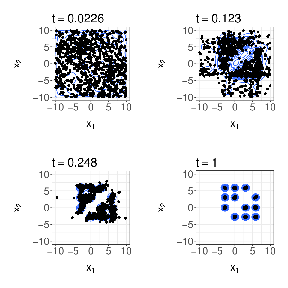
As the full conditional distributions of the posterior are not in the exponential family, we employ the Gibbs velocity field (23)-(24) for one-dimensional components. Using a composite trapezoidal rule with quadrature points and the default ODE solver from the deSolve R package, we compare the time evolution of prior samples under the Gibbs flow with the output of a standard SMC sampler with many particles as the reference truth in Figure 1. The performance of the Gibbs flow for this challenging problem is striking as the samples reach all modes.
This is also seen in Figure 2 that shows all pairwise marginal posterior distributions on (note that each of these marginals admits well-separated modes).

To corroborate these observations, we simulate another independent Gibbs flow samples and display the proportion of samples in each of the modes in Figure 3.

The uniformity of these proportions is then tested using a Pearson’s Chi-squared goodness-of-fit test, which gives a p-value of . Next, we examine how well the distribution of Gibbs flow samples matches the posterior distribution in the left panel of Figure 4. Although there is good agreement between these distributions, there is still some discrepancy which is analyzed in Proposition 4. In the right panel of Figure 4, we show that this difference can be reduced by combining the Gibbs flow with Hamiltonian Monte Carlo (HMC) kernels33 3 Here we apply a Hamiltonian Monte Carlo kernel between time intervals of . We use a step size of for the leapfrog integrator and an integration time of ., as discussed in Section 4.3.


5.2 Variance component models
We now apply our proposed methodology to variance component models, which is typical of problems in Bayesian statistics where one would employ a Gibbs sampler [23, 47]. Firstly, there are two hyperparameters with prior distributions and , where (and ) denotes the inverse Gamma distribution (and density) with shape parameter and scale parameter . Following [47], we adopt an improper prior for and a flat or vague prior for . Given these hyperparameters, there are location parameters that are conditionally independent and distributed as for . With these parameters, observations at each location are modeled as conditionally independent and distributed as for where is estimated empirically. We will write as the observed dataset.
In this application, the improper prior (with a possibly negative value of ) is
| (37) |
and the likelihood function is for . To employ the methodology described in Section 2.1, we set as the parameters to be inferred and consider the following “artificial” prior distribution
| (38) |
to initialize our method, for some fixed . The corresponding “artificial” likelihood function that would yield the desired posterior is
Given these choices, which are necessary to deal with the improper prior (37), we can then define the curve of distributions in (2).
It can be shown that the full conditional distributions of are
| (39) |
where the summary statistics are given in Appendix H. Since these full conditionals lie in the exponential family, we can exploit such analytical tractability to determine a Gibbs velocity field. For the parameter , we use (19) which reduces to
| (40) |
where and denote the time derivatives of and respectively,
and is the digamma function44 4 We evaluate this function using the digamma function in the R base package.. For parameters and which have Gaussian full conditional distributions, the corresponding components of the Gibbs velocity field are more explicit
| (41) | ||||
| (42) |
where and denote the time derivatives of and respectively. To approximate the Gibbs flow, we update the parameter at time step using the Euler discretization (27), which defines the map
where denotes an approximation of (40) using a composite trapezoidal rule with quadrature points. To update the parameter or conditionally on other parameters, since the solution of (28) under the linear velocity (41) or (42) is tractable, we have
for . In contrast to the generic expressions in (23)-(24), approximating the Gibbs flow for this model only requires computing summary statistics and evaluating inverse Gamma densities.
We consider a dataset of baseball players’ batting averages () taken from [51, Table 1]. In this case, the number of parameters to be inferred is . Following [47], we adopt the empirical estimate and a prior specification corresponding to . We initialize the Gibbs flow using an “artificial” prior distribution (38) with . In Figure 5, we display the performance of the resulting GF-SIS (Algorithm 1) using samples and time steps.


To improve performance with fixed and , we combine approximate Gibbs flow with HMC kernels55 5 We apply a Hamiltonian Monte Carlo kernel at each time step. To achieve suitable acceptance probabilities, we use a step size of for the leapfrog integrator and an integration time of . within GF-AIS (Algorithm 2): this increases the ESS% from to on average, and reduces the variance of the log-marginal likelihood estimator by a factor of , at the expense of times the compute time of GF-SIS. As competing algorithm, we consider AIS with the same , and HMC kernels as GF-AIS, but we increase the number of HMC iterations at each time step to match the computational time of GF-AIS, so as to ensure a fair comparison. Based on independent repetitions of all three algorithms, the sample variance of log-marginal likelihood estimates relative to AIS was observed to be and times smaller for GF-SIS and GF-AIS respectively.
We then investigate how the performance of these algorithms behaves with dimension on simulated data. The model specification and algorithmic settings remain the same as we scale , with the exception of increasing time steps linearly with and decreasing the step size of the leapfrog integrator in HMC to achieve stable acceptance probabilities66 6 For , we use steps of the leapfrog integrator with step size respectively. . Like before, we select the number of HMC iterations in AIS to match the compute time of GF-AIS; both algorithms require approximately times more compute time than GF-SIS as varies. Figure 6 summarizes how the performance of these algorithms scale with dimension. Relative to standard AIS, GF-SIS performed better in all of the observed dimensions despite costing less compute time, and GF-AIS offers much better ESS% and variance reduction of several orders at a fixed computational cost.


5.3 Log-Gaussian Cox point processes
Lastly, we present an application of our methodology on a model from spatial statistics. In particular, we consider Bayesian inference for log-Gaussian Cox point processes on a dataset77 7 The dataset can be found in the R package spatstat as finpines. concerning the locations of Scots pine saplings in a natural forest in Finland [37, 13, 25]. The actual square plot of square metres is standardized to the unit square and discretized into a regular grid. Given a latent intensity process , the number of points in each cell for are modeled as conditionally independent and Poisson distributed with mean , where is the area of each cell. The prior distribution of the intensity is specified by the relation for , where is a Gaussian process with constant mean and exponential covariance function for and . We will adopt the parameter values , and estimated by [37]. This application corresponds to working in dimension with a prior distribution of where and a likelihood function of , where denotes the dataset.
We will apply the methodology described in Section 2.1 with initialization from the prior distribution or a Gaussian approximation of the posterior distribution; given by either a mean field variational Bayes (VB) approximation [52] , or of the form , where are fitted using expectation-propagation (EP) [36], as advocated in [12]. To accommodate these choices, we take as “artificial” likelihood function to define the curve of distributions in (2). Although the full conditional distributions of are not in the exponential family, computation of the Gibbs velocity field (23)-(24) for one-dimensional components can be greatly simplified by rewriting
| (43) |
where and
for , and noting that the full conditional distributions and are univariate Gaussians that can be precomputed. We approximate (43) using a composite trapezoidal rule with quadrature points, and the Gibbs flow using the Euler discretization (27), which defines the map for time step and component .
We first consider initialization from the prior and vary the spatial resolution by taking . Figure 7 displays the performance of GF-SIS (Algorithm 1) using samples and as we increase the time steps with dimension correspondingly. To obtain better performance for the same number of samples and time steps , we combine approximate Gibbs flow with Riemann manifold Hamiltonian Monte Carlo (RM-HMC) kernels88 8 We apply a Riemann manifold Hamiltonian Monte Carlo kernel at each time step, with a leapfrog integrator step size of 0.25 and an integration time of 2.5. that employ the metric tensor [25], where denotes the identity matrix. Although the resulting GF-AIS (Algorithm 2) requires approximately more compute time than GF-SIS as dimension increases, it is apparent from Figure 7 that it improves algorithmic performance by several orders of magnitude. Like before, we compare GF-AIS to an AIS with the same , and RM-HMC kernels, but to ensure a fair comparison, the number of RM-HMC iterations at each time step is increased to match computational time. The results summarized in Figure 7 indicate that GF-AIS can offer very significant numerical gains over standard AIS in all three dimensions considered.


Lastly, we investigate the impact of the initial distribution for a spatial resolution of . Figure 8 shows that initial distributions that are “closer” to the posterior than the prior typically lead to better algorithmic performance. Interestingly, due to the nature of the Gibbs flow approximation, we find that an EP approximation of the posterior provides a better initialization than a VB approximation.


References
- [1] L. Ambrosio. Transport equation and Cauchy problem for BV vector fields. Inventiones Mathematicae, 158(2):227–260, 2004.
- [2] L. Ambrosio, N. Gigli and G. Savaré. Gradient Flows in Metric Spaces And in the Space of Probability Measures. Lectures in Mathematics ETH Zurich. Birkhauser, 2005.
- [3] A. R. Barron and X. Luo. Adaptive annealing. In Proceedings of the Allerton Conference on Communications, Computation and Control, 665–673, 2007.
- [4] J. D. Benamou and Y. Brenier. A computational fluid mechanics solution to the Monge-Kantorovich mass transfer problem. Numerische Mathematik, 84(3):375–393, 2000.
- [5] K. Bergemann and S. Reich. An ensemble Kalman-Bucy filter for continuous data assimilation. Meteorologische Zeitschrift, 21(3):213–219, 2012.
- [6] M. J. Betancourt. Adiabatic Monte Carlo. arXiv preprint arXiv:1405.3489, 2014.
- [7] O. Bokanowski and B. Grébert. Deformations of density functions in molecular quantum chemistry. Journal of Mathematical Physics, 37(4):1553–1573, 1996.
- [8] P. Bunch and S. J. Godsill. Approximations of the optimal importance density using Gaussian particle flow importance sampling. Journal of the American Statistical Association, 111(514): 748–762, 2016.
- [9] G. Celeux, M. Hurn and C. P. Robert. Computational and Inferential Difficulties with Mixture Posterior Distributions. Journal of the American Statistical Association, 95(451):957–970, 2000.
- [10] A. Chkifa, A. Cohen and C. Schwab. Breaking the curse of dimensionality in sparse polynomial approximation of parametric PDEs. Journal de Mathématiques Pures et Appliquéees, 103(2):400–428, 2015.
- [11] N. Chopin. A sequential particle filter method for static models. Biometrika, 89(3):539–552, 2002.
- [12] N. Chopin and J. Ridgway. Leave Pima Indians alone: Binary regression as a benchmark for Bayesian computation. Statistical Science, 32(1):64–87, 2017.
- [13] O. F. Christensen, G. O. Roberts and J. S. Rosenthal. Scaling limits for the transient phase of local Metropolis–Hastings algorithms. Journal of the Royal Statistical Society: Series B (Statistical Methodology), 67(2):253–268, 2005.
- [14] D. Crisan and J. Xiong. Approximate McKean–Vlasov representations for a class of SPDEs. Stochastics, 82(1):53–68, 2010.
- [15] G. E. Crooks. Nonequilibrium measurements of free energy differences for microscopically reversible Markovian systems. Journal of Statistical Physics, 90(5–6):1481–1487, 1998.
- [16] B. Dacorogna and J. Moser. On a partial differential equation involving the Jacobian determinant. Annales de l’Institut Henri Poincaré C (Analyse non linéaire), 7:1–26, 1990.
- [17] W. Dahmen, R. Devore, L. Grasedyck and E. Süli. Tensor-sparsity of solutions to high-dimensional elliptic partial differential equations. Foundations of Computational Mathematics, 1–62, 2014.
- [18] F. Daum and J. Huang. Particle flow and Monge-Kantorovich transport. In Proceedings Conference on Information Fusion, 135–142, 2012.
- [19] P. Del Moral, A. Doucet and A. Jasra. Sequential Monte Carlo samplers. Journal of the Royal Statistical Society: Series B (Statistical Methodology), 68(3):411–436, 2006.
- [20] R. J. DiPerna and P. L. Lions. Ordinary differential equations, transport theory and Sobolev spaces. Inventiones Mathematicae, 98(3):511–547, 1989.
- [21] T. A. El Moselhy and Y. M. Marzouk. Bayesian inference with optimal maps. Journal of Computational Physics, 231(23):7815–7850, 2012.
- [22] C. W. Gardiner. Handbook of Stochastic Methods for Physics, Chemistry and the Natural Sciences. 2nd edition, Springer, 2002.
- [23] A. E. Gelfand and A. F. Smith. Sampling-based approaches to calculating marginal densities. Journal of the American Statistical Association, 85(410):398–409, 1990.
- [24] A. Gelman and X. L. Meng. Simulating normalizing constants: From importance sampling to bridge sampling to path sampling. Statistical Science, 13(2):163–185, 1998.
- [25] M. Girolami and B. Calderhead. Riemann manifold Langevin and Hamiltonian Monte Carlo methods. Journal of the Royal Statistical Society: Series B (Statistical Methodology), 73(2):123–214, 2011.
- [26] R. E. Greene and K. Shiohama. Diffeomorphisms and volume-preserving embeddings of noncompact manifolds. Transactions of the American Mathematical Society, 255:403–403, 1979.
- [27] J. Han and Q. Liu. Stein Variational Adaptive Importance Sampling. In Uncertainty in Artificial Intelligence, 2017.
- [28] A. Iserles. A First Course in the Numerical Analysis of Differential Equations. Cambridge University Press, 2009.
- [29] C. Jarzynski. Nonequilibrium equality for free energy differences. Physical Review Letters, 78(14), 2690, 1997.
- [30] S. Kim, R. Ma, D. Mesa and T. P. Coleman. Efficient Bayesian inference methods via convex optimization and optimal transport. In IEEE International Symposium on Information Theory Proceedings, pages 2259–2263. IEEE, 2013.
- [31] S. Kirkpatrick, C. D. Gelatt and M. P. Vecchi. Optimization by simulated annealing. Science, 220(4598):671–680, 1983.
- [32] A. Kong, J. S. Liu and W. H. Wong. Sequential imputations and Bayesian missing data problems. Journal of the American Statistical Association, 89(425):278–288, 1994.
- [33] A. Lee, C. Yau, M. B. Giles, A. Doucet and C. C. Holmes. On the utility of graphics cards to perform massively parallel simulation of advanced Monte Carlo methods. Journal of Computational and Graphical Statistics, 19(4):769–789, 2010.
- [34] Q. Liu and D. Wang. Stein variational gradient descent: A general purpose Bayesian inference algorithm. In Advances in Neural Information Processing Systems, pages 2370–2378, 2016.
- [35] X. L. Meng and S. Schilling. Warp bridge sampling. Journal of Computational and Graphical Statistics, 11(3):552–586, 2002.
- [36] T. Minka. Expectation propagation for approximate Bayesian inference. Proceedings of Uncertainty in Artificial Intelligence, 17:362–369, 2001.
- [37] J. Møller, A. R. Syversveen and R. P. Waagepetersen. Log Gaussian Cox processes. Scandinavian Journal of Statistics, 25(3):451–482, 1998.
- [38] J. Moser. On the volume elements on a manifold. Transactions of the American Mathematical Society, 120(2):286–294, 1965.
- [39] R. M. Neal. Annealed importance sampling. Statistics and Computing, 11(2):125–139, 2001.
- [40] E. Novak and H. Wozniakowski. Approximation of infinitely differentiable multivariate functions is intractable. Journal of Complexity, 25(4):398–404, 2009.
- [41] C. J. Oates, T. Papamarkou and M. Girolami. The controlled thermodynamic integral for Bayesian model evidence evaluation. Journal of the American Statistical Association, 111(514):634–645, 2016.
- [42] M. Parno, T. Moselhy and Y. M. Marzouk. A multiscale strategy for Bayesian inference using transport maps. SIAM/ASA Journal on Uncertainty Quantification, 4(1):1160–1190, 2016.
- [43] M. Parno and Y. M. Marzouk. Transport map accelerated Markov chain Monte Carlo. SIAM/ASA Journal on Uncertainty Quantification, 6(2):645–682, 2018.
- [44] G. Peyré and M. Cuturi. Computational optimal transport. Foundations and Trends in Machine Learning, 11(5–6):355–607, 2019.
- [45] S. Reich. A dynamical systems framework for intermittent data assimilation. BIT Numerical Analysis, 51(1):235–249, 2011.
- [46] S. Reich. A Gaussian-mixture ensemble transform filter. Quarterly Journal of the Royal Meteorological Society, 138(662):222–233, 2012.
- [47] J. S. Rosenthal. Analysis of the Gibbs sampler for a model related to James-Stein estimators. Statistics and Computing, 6(3):269–275, 1996.
- [48] S. Reich and C. J. Cotter. Probabilistic Forecasting and Bayesian Data Assimilation. Cambridge University Press, 2015.
- [49] A. Spantini, D. Bigoni and Y. M. Marzouk. Inference via low-dimensional couplings. Journal of Machine Learning Research, 19(66):1–71, 2018.
- [50] Y. Tao, P. G. Mehta and S. P. Meyn. Feedback particle filter. IEEE Transactions on Automatic Control, 58(10):2465–2480, 2013.
- [51] C. N. Morris. Parametric empirical Bayes inference: theory and applications. Journal of the American Statistical Association, 78(381):47–55, 1983.
- [52] M. Teng, F. Nathoo, and T. D Johnson. Bayesian computation for Log-Gaussian Cox processes: a comparative analysis of methods. Journal of Statistical Computation and Simulation, 87(11), 2227–2252, 2017.
- [53] S. Vaikuntanathan and C. Jarzynski. Escorted free energy simulations: Improving convergence by reducing dissipation. Physical Review Letters, 100(19), 190601, 2008.
- [54] S. Vaikuntanathan and C. Jarzynski. Escorted free energy simulations. Journal of Chemical Physics, 134(5), 054107, 2011.
- [55] C. Villani. Optimal Transport: Old and New. Springer Berlin Heidelberg, 2008.
- [56] W. Walter. Ordinary Differential Equations. Springer, 1998.
- [57] Y. Zhou, A. M. Johansen and J. A. D. Aston. Towards automatic model comparison: An adaptive sequential Monte Carlo approach. Journal of Computational and Graphical Statistics, 25(3):701–726, 2016.
Appendix A Informal derivation of Liouville’s equation
Consider a -dimensional hyper-rectangle , defined formally as the Cartesian product of intervals for and some small , to be thought of as an infinitesimal control volume at a point .
If we perceive particles as constituents of a fluid representing probability mass, then the fluid flow driven by a velocity field will cause the probability mass in to change. Along the axis, for sufficiently small , this change is given by the difference between the rate at which mass flows into
| (44) |
and the rate at which mass flows out of
| (45) |
where denote the canonical basis vectors in . In fluid dynamics terminology, the leading terms in (44) and (45) are simply the density multiplied by the volume metric flow rate in and out of the control volume respectively.
Appendix B Flow transport problem
In this section, we supply additional details behind the validity of the flow transport problem. We first establish a preliminary result about the curve of distributions (2).
Lemma 1.
The curve of distributions defined in (2) is narrowly continuous, i.e. for any bounded function and any sequence such that we have
| (49) |
Proof.
Using the dominated convergence theorem with dominating function
shows that is continuous on . Together with continuity of , it then follows that for each . Hence for any bounded function and any sequence such that , we have pointwise. Note that
| (50) |
Since is continuous on , the infimum in (50) is attained and is strictly positive under positivity assumptions made on and . Hence the upper bound in (50) is integrable and by the dominated convergence theorem, (49) follows. ∎
We now introduce the notion of weak solutions which is needed to establish Theorem 1.
Definition 1.
A curve of distributions is a weak solution of (8) if
| (51) |
for all compactly supported , where denotes the inner product in .
Proof of Theorem 1.
It is worth noting that converse of Theorem 1 also holds under the same conditions [2, Lemma 8.1.6]. These two results describe an equivalence between the Eulerian perspective characterized by Liouville’s PDE (8) and the Lagrangian perspective described in terms of particle trajectories governed by the ODE (6). It is possible to weaken Assumption A1; see [20] for earlier work and [1], [2, Theorem 8.2.1] for recent advances.
Appendix C Solving the flow transport problem
In this section, we first detail the proofs of Propositions 1-2 before giving additional remarks on our solution to the flow transport problem.
Proof of Proposition 1.
Using continuity of and positivity of , an application of the first fundamental theorem of calculus shows that satisfies (9). The assumptions on and imply hence Assumption A1 of Theorem 1 holds. The integrability Assumption A2 in Theorem 1 follows from the prescribed tail behaviour of uniformly over . Therefore the assumptions of Theorem 1 hold and solves the flow transport problem on . To see that (10) is indeed the minimal kinetic energy solution, we note that the optimality condition in [45, 46] requires existence of a function such that . This follows as a consequence of working on since we may set . ∎
Proof of Proposition 2.
The arguments are similar to those used in Proposition 1. By straightforward verification satisfies (9):
The penultimate line applies the first fundamental theorem of calculus and the final equality comes from the telescopic sum. The assumptions on and imply hence Assumption A1 of Theorem 1 holds. The integrability Assumption A2 in Theorem 1 follows from the prescribed tail behaviour of uniformly over . Therefore the assumptions of Theorem 1 hold and solves the flow transport problem on . ∎
We note that the velocity field defined in (14)-(15) satisfies as for each by construction. The tail behaviour prescribed in Proposition 2 assumes that this decay happens fast enough to ensure the integrability Assumption A2 in Theorem 1.
Suppose that the curve of distributions (2) factorize into independent one-dimensional components, i.e.
where for , denotes the marginal distribution of , the corresponding likelihood function and . In this case, the time evolution along the curve for each marginal distribution is given by
where . We now show that the velocity field in (14)-(15) would reduce to (16), which is the minimal kinetic energy solution of the following system of uncoupled Liouville PDEs
for , given by Proposition 1 for each marginal distribution. From (14), for
| (52) |
and from (15)
| (53) |
Appendix D Gibbs flow approximation
This section concerns properties of the Gibbs flow approximation. We first give the proof of Proposition 3.
Proof of Proposition 3.
By Assumption A3, which implies that it is locally Lipschitz. With local Lipschitzness, we need to establish that the solution of (20), with initial condition , is bounded whenever it exists to complete the proof. Boundedness will be obtained by showing that is a Lyapunov function. Define for and note that as under our assumption. Using Assumption A4, there exists such that
| (54) |
for all such that . It follows that where . ∎
We now show that Assumption A4 can be verified for the Gibbs velocity field in the case by choosing . Clearly, and as . By assumption, as so there exists such that for . It follows from (3) that
and therefore
for . Next we detail the proof of Proposition 4.
Proof of Proposition 4.
Let denote the velocity field (14)-(15) in Proposition 2 and recall that it satisfies the Liouville equation (9). Define as the difference for . By taking the difference between (9) and
and introducing a cross term, we obtain
Multiplying throughout by and applying chain rule yields
We then integrate by parts to obtain
noting that the boundary term vanishes by Assumption A5. Using Young’s inequality gives
| (55) | ||||
for any . Since , integrating both sides of (55) on yields
Now applying Gronwall’s lemma on the time interval combined with the fact that is non-decreasing
Lastly, minimizing this upper bound w.r.t. gives (22). ∎
Appendix E Numerical integration of the Gibbs flow
In the following, we will show that the numerical integration scheme (29) is a first order method, i.e. the global error
for all , if the step size is sufficiently small. For ease of presentation, we will consider components; extension to the case is straightforward but less instructive. We consider the case where the maps are defined by Euler discretizations, i.e.
| (56) |
By a Taylor expansion, the case where and are defined by analytically tractable flows (when the other component is fixed) differs from (56) by an term; therefore, it will be apparent that there is no loss of generality in considering Euler discretizations. We will assume that the (approximated) Gibbs velocity field is Lipschitz continuous, i.e. for all .
For each step size , we define the function as
which allows us to express the numerical integration scheme as a one-step method
| (57) |
We note that is also Lipschitz continuous with a Lipschitz constant that depends on . We first examine the local truncation error
| (58) |
Assuming that the solution defined by (26) satisfies , by Taylor’s theorem
for some , where denotes the second derivative of . Substituting this expansion into (58), we have by Lipschitz continuity of and the form of (56) that
Defining and , the local truncation errors are bounded by
| (59) |
To relate local truncation errors to global errors, we rewrite (58) as
Appendix F Gibbs flow samplers with resampling
In this section, we detail modifications of Algorithms 1-2 to incorporate resampling at every time step. We will use the notation to denote a resampling operation based on a vector of normalized weights , i.e. for all and . In this case, Algorithm 3 replaces Algorithm 1 and Algorithm 4 replaces Algorithm 2. The normalizing constant estimators returned by Algorithms 3-4 are both unbiased estimators of the marginal likelihood . To approximate expectations of the form , we will use from the output of Algorithm 3, and from the output of Algorithm 4.
Input: prior , likelihood , inverse temperature , step size , and Gibbs velocity field .
For time step
For
(a) sample ;
(b) set , and ;
(c) set and .
For time step
For
For
(d) set using Section 4.1;
(e) compute using Section 4.2;
(f) set and ;
(g) compute unnormalized weights
(h) compute normalized weights ;
(i) sample ancestor index ;
(j) compute effective sample size ;
(k) compute normalizing constant estimator .
Output: samples , ancestors and normalizing constant estimator .
Input: prior , likelihood , inverse temperature , step size , Gibbs velocity field , MCMC kernels .
For time step
For
(a) sample and set ;
(b) set and ;
(c) set and .
For time step
For
For
(d) set using Section 4.1;
(e) compute using Section 4.2;
(f) set and ;
(g) compute unnormalized weights
(h) compute normalized weights ;
(i) sample ancestor index ;
(j) sample from -invariant MCMC kernel;
(k) compute effective sample size ;
(l) compute normalizing constant estimator .
Output: samples and normalizing constant estimator .
Appendix G Flow transports for curve of Gaussian distributions
In this section, we illustrate the flow transports introduced in Section 3 on a curve of Gaussian distributions.
G.1 Curve of Gaussian distributions
Consider the prior distribution and likelihood function
with symmetric positive definite and observation . By conjugacy, the curve of distributions defined in (2) lies in the Gaussian family, i.e. for with
| (60) |
and the expected log-likelihood (4) is
| (61) |
where denotes the trace of a square matrix . In this Gaussian setting, the minimum kinetic energy solution to the flow transport problem [5, 46, 48]
| (62) |
where
is analytically tractable and is given by
| (63) |
G.2 Univariate case
As noted in Proposition 1, the velocity field in (10) corresponds exactly to (62) when . For a more concrete example, we shall consider . The curve of distributions in Appendix G.1 is given by , so as time progresses, we expect particles to have a mean-reverting behaviour towards the origin. This is indeed the case in (63) which gives a linear mean-reverting drift . Figure 9 also illustrates this behaviour with the steering property mentioned in Section 3.1: since for all , reversion to the stable stationary point at the origin dictates that for and for .

G.3 Pathological case
Using the same arguments in the proof of Propositions 1-2, the velocity field given in (13) satisfies Liouville equation (9) whenever . However, Theorem 1 does not apply as as for any , so Assumption A2 does not hold. On a simple Gaussian example detailed below, we will establish that (13) does not solve the flow transport problem by showing that an ODE with velocity field would yield divergent particle trajectories.
Consider and the curve of distributions in Appendix G.1 with parameters and . This setup corresponds to independent components that are marginally distributed according to the univariate Gaussian model of Appendix G.2. Hence we would expect a particle under a valid flow transport to have a mean-reverting behaviour towards the origin. The velocity field in (13) has the form
| (64) |
for and , where and denotes the marginal CDFs. We note that the two components of the velocity field are coupled.
Now consider with . We investigate the behaviour of particles in the upper-right quadrant of the space. For each , define the sets and ; noting that , it follows from (64) that for any . Since , we can conclude that there exist particle trajectories which only move farther away from the origin with positive probability. Analytical tractability in this simple example allows us to strengthen the previous statement and show that these trajectories in fact blow up in finite time. We start by seeking a lower bound on ; by symmetry, it suffices to consider only the first component. On the set , we have , hence
| (65) |
where . Now consider an uncoupled system of ODEs with velocity field
| (66) |
and note that its solution , corresponding to an initial condition , diverges as . Define the set . Noting that is locally Lipschitz and component-wise increasing, the comparison theorem [56, Theorem III.10.XII (b), p. 112] implies that a particle starting in and evolving under (64) has a trajectory that explodes before . Since , we conclude the claim that there exist divergent particle trajectories with positive probability.
G.4 Multivariate case
Consider and the curve of distributions in Appendix G.1 with parameters and . In this setting, as time progresses, the independent prior distribution simultaneously gets deformed and translated. Figure 10 illustrates that, on average, particles driven by (63) require less kinetic energy than that of (14)-(15). However, in the general non-Gaussian case, obtaining the minimal kinetic energy velocity field requires numerical resolution of an elliptic PDE.

G.5 Gibbs flow approximation
To illustrate the nature of the Gibbs flow approximation (19), we consider the setting in Appendix G.4 and observe the -error analyzed in Proposition 4 at varying degrees of correlation, induced by the parameter , and extremality of the observation . The left panel of Figure 11 shows that while performance degrades with , as expected from our construction, the approximation is able to exploit any local independence structure in the target distributions, thus keeping the error reasonably small for moderate degrees of correlation. The right panel of Figure 11 reveals the inadequacy of the approximation when the overlap between the prior distribution and the likelihood function decreases, which is also to be expected.

Appendix H Expressions for variance component models
Appendix I Toy examples
In this section, we consider two additional examples to investigate the quality of the Gibbs flow approximation.
I.1 Banana-shaped posterior
First we consider a banana-shaped posterior distribution on , induced by the prior distribution
| (67) |
and the likelihood function
that is defined by the Rosenbrock function. The log-likelihood function is not concave and has a global maximum at . Therefore the parameter controls the overlap between the prior distribution and the likelihood function. The parameter specifies the strength of the dependency between the variables and : having would give an independent posterior distribution , while larger values of would induce more dependent posterior distributions. In the following, we will consider and .
Using a composite trapezoidal rule with quadrature points and the Euler discretization (27) with time steps, the upper left panel of Figure 12 shows the terminal position of samples against contours of the prior and posterior densities. To improve performance, we either combine the Gibbs flow with HMC kernels within GF-AIS (Algorithm 2) or include weighting and resampling steps within GF-SISR (Algorithm 3). The upper right panel of Figure 12 illustrates the benefits of adding MCMC moves to prevent accumulation of errors; the lower left panel of Figure 12 shows that weighting and resampling offers improvement at the expense of sample diversity, as this results in a duplicate set of samples. Lastly, the lower right panel of Figure 12 demonstrates that sample diversity can be rejuvenated by combining resampling with MCMC moves within GF-SMC (Algorithm 4).


I.2 Gaussian mixture posterior
Next we examine a multimodal posterior distribution on , given by the prior distribution (67) and a likelihood function of the form
The weights satisfy for and , the observations are
for some location parameter and , with
for some correlation parameter . It can be shown that the posterior distribution is a Gaussian mixture
with mean vectors for and covariance matrices
We will set , , and vary .
To approximate the Gibbs flow, we employ a composite trapezoidal rule with quadrature points and the default ODE solver from the deSolve R package. To estimate the mixture weights using the terminal positions of samples under the Gibbs flow, we run a -means clustering algorithm with clusters and initialization at the posterior means . The proportion of samples in each of the four clusters are taken as estimates of and reported in Table 1 for the values of that are considered. We also compute the p-values of Pearson’s Chi-squared goodness-of-fit tests under the null hypothesis that the population weights are equal to . Figure 13 displays the terminal position of samples with color-coding to show the clustering for various values of , against contours of the prior and posterior densities.
It is apparent from Table 1 that the estimation error increases with the correlation parameter , which is to be expected. The relative error in estimating ranges from to , while that of ranges from to . The p-values that were computed with samples, on the other hand, indicate poor approximation of the true values for all non-zero values of . Lastly, we note that one can improve the quality of the Gibbs flow approximation by adding MCMC moves or weighting and resampling steps, as discussed above.
| p-value | |||||
|---|---|---|---|---|---|


