Bayesian GARMA Models for Count Data

Suppose that $y_{t}|\textit{F}_{t-1}$ follows a Poisson distribution with mean $\mu_{t}$. Then,

and $Y_{t}|\textit{F}_{t-1}$ has distribution in the exponential family with $\varphi=1$, $\alpha_{t}=\log(\mu_{t})$, $b(\alpha_{t})=\exp(\alpha_{t})$, $c(y_{t},\varphi)=-\log(y_{t}!)$ and $\nu(\mu_{t})=\mu_{t}$. The canonical link function for this model is the logarithmic function, so that the linear predictor is given by,

Where $y_{t-j}^{*}=\max(y_{t-j},c),0<c<1$. The Poisson GARMA model is defined by equations (3) and (4).

Suppose that $y_{t}|\textit{F}_{t-1}$ follows a binomial distribution with mean $\mu_{t}$. Then,

The canonical link function for this model is the logarithmic function. The linear predictor is given by,

with $y_{t-j}^{*}=\max(y_{t-j},c),0<c<1$, and $m$ is known.

Let $y_{t}$ a time series such that $y_{t}|\textit{F}_{t-1}\sim NB(k,\mu_{t})$. Then,

which belongs to the exponential family with $k$ known. The link function for this model is the logarithmic function

with $y_{t-j}^{*}=\max(y_{t-j},c),0<c<1$.

Using the logarithmic in link function to guarantee positive values for any values of the vectors $\boldsymbol{\beta}=(\beta_{1},\ldots,\beta_{m})$, $\Phi=(\phi_{1},\ldots,\phi_{p})$ and $\Theta=(\theta_{1},\ldots,\theta_{q})$.$\beta$, $\phi_{i}$. Thus, a multivariate Gaussian prior will be proposed for each parameter.

where $\boldsymbol{\mu_{0}},\boldsymbol{\mu_{1}},\boldsymbol{\mu_{1}}$ are vectors with length $m$, $p$ and $q$ respectively, $\sigma_{0}^{2}$, $\sigma_{1}^{2}$ and $\sigma_{1}^{2}$ represent the prior variance and $\boldsymbol{I_{0}}$, $\boldsymbol{I_{1}}$ and $\boldsymbol{I_{2}}$ are $m\times m$, $p\times p$ and $q\times q$ identity matrices respectively. The construction of the multivariate Gaussian depends on hyper parameters, when there is no prior knowledge on these parameters it can be considered a vary large variance making the prior densities flats. The partial likelihood function for GARMA models can be constructed as follows

where $\alpha_{t}=g(\mu_{t})$, which represent the link function given by

for all $t=r+1,\ldots,n$.

The posterior density is obtained combining the likelihood function with the prior densities. Let the vector $\boldsymbol{Y}=(y_{t},y_{t-1},\dots,y_{1},x_{t},x_{t-1},\dots,x_{1},\dots)$ represent the necessary information to construct the likelihood function. The posterior density is then given by,

An important aspect of our Bayesian approach to GARMA models is the hability to forecasting future values of the time series, $y_{t+h}$, $h\geq 1$ given all the information available until time $t$. To evaluate this forecasting it is necessary to find the predictive density function $p(y_{t+h}|Y)$.

Denoting the information set $\widehat{\textit{F}}_{t+h}=(\widehat{x}_{t+h},\dots,x_{t},x_{t-1},\dots,$ $\widehat{y}_{t+h-1},\dots,y_{t},$ $y_{t-1},\dots$ $\widehat{\mu}_{t+h-1}$,$\dots,$ $\mu_{t},\mu_{t-1},\dots)$, where $\widehat{y}_{t+h-i}=y_{t+h-i}$, if $h\leq i$, else $\widehat{y}_{t+h-i}=E\{y_{t+h-i}|\widehat{\textit{F}}_{t+h-i}\}$, $i=1,2,\ldots h+1$. The general idea is that $\widehat{\textit{F}}_{t+h}$ contains all the data observed until the time $t$, for the future time $t+h$, $h\geq 1$, the set $\widehat{\textit{F}}_{t+h}$ is completed with forecasts of necessary information to estimate $y_{t+h}$. Starting with,

The conditional mean and variance of $y_{t+h}$ given $\widehat{\textit{F}}_{t+h}$ is represented by the terms $\widehat{\mu}_{t+h}=$ $E(y_{t+h}|\widehat{\textit{F}}_{t+h})$ $=b^{\prime}(\alpha_{t+h})$ and $Var(y_{t+h}|\textit{F}_{t+h})=$ $\varphi{b^{\prime\prime}}(\alpha_{t+h})$. The $\mu_{t+h}$, is related to the predictor, $\eta_{t+h}$, by a twice-differentiable one-to-one monotonic link function $g(\cdot)$. The linear predictor for the GARMA model is given by,

With the equation (7) and posterior density (6), the predictive density for $y_{t+h}$ can be written as,

The aim is to determine the predictive density using the MCMC algorithm, thus

Given the predictive density, the next step is to evaluate the prediction, $E(y_{t+h}|\widehat{\textit{F}}_{t+h})=\hat{y}_{t+h}$.

which can in turn be rewritten as

Credible intervals for $\widehat{y}_{t+h}$ can be calculated using the $100\alpha\%$, and $100(1-\alpha)\%$ quantiles of the MCMC sample $\mu^{(k)}_{t+h}$, with $k=1,\ldots,Q$. An approach to estimate the credible interval of $\widehat{y}_{t+h}$ is the Highest Posterior Density (HPD), see ?). A $100(1-\alpha)\%$ HPD region for $\widehat{y}_{t+h}$ are a subset $C\in R$ defined by $C=\{y_{t+h}:p(y_{t+h}|\widehat{\textit{F}}_{t+h})\geq\kappa\}$, where $\kappa$ is the largest number such that

We can use the $\widehat{p}(y_{t+h}|\widehat{\textit{F}}_{t+h})$ MCMC estimates, given by the equation (9), to estimate the $100(1-\alpha)\%$ HPD region. We used the following algorithm to calculate the credible intervals for the predictions.

• 1.

  Let a sequence of forecast values $\widehat{y}_{t+h}$ for $h=1,\ldots,H$.

• 2.

  Take $h=1$, $k=0$, $y_{t+h}^{(0)}=0$, $S_{t+h}^{(0)}=0$ and also initiate $LB=0$, $UB$=0.

• 3.

  Using the initial values evaluate the equation:

  $$f(y_{t+h}^{(k)}|\beta^{(j)},\Phi^{(j)},\Theta^{(j)},\widehat{\textit{F}}_{t+h})=\exp\left(\frac{y_{t+h}^{(k)}\alpha_{t+h}^{(j)}-b(\alpha_{t+h}^{(j)})}{\varphi}+d(y_{t+h}^{(k)},\varphi)\right),$$

  and also,

  $$\widehat{p}(y_{t+h}^{(k)}|\widehat{\textit{F}}_{t+h})=\frac{1}{Q}\sum_{j=1}^{Q}f(y_{t+h}^{(k)}|\beta^{(j)},{\Phi^{(j)}},{\Theta^{(j)}},\widehat{\textit{F}}_{t+h}).$$

• 4.

  Using $\widehat{p}(y_{t+h}^{(k)}|\widehat{\textit{F}}_{t+h})$ compute $S_{t+h}^{(k+1)}$ with

  $$S_{t+h}^{(k+1)}=S_{t+h}^{(k)}+\widehat{p}(y_{t+h}^{(k)}|\widehat{\textit{F}}_{t+h})$$

• 5.

  If $LB=0$ and $S_{t+h}^{(k+1)}\geq\delta$, $\rightarrow$ $y_{t+h,\delta}=y_{t+h}^{(k)}$ and $LB=1$.

• 6.

  If $UB=0$ and $S_{t+h}^{(k+1)}\leq(1-\delta)$, $\rightarrow$ $y_{t+h,(1-\delta)}=y_{t+h}^{(k)}$ and $UB=1$.

• 7.

  If $LB=0$ or $UB=0$, take $k=k+1$ and $y_{t+h}^{(k)}=y_{t+h}^{(k-1)}+1$, repeat steps 3 and 4 until $LB=1$ and $UB=1$.

The percentiles $100\delta\%$ and $100(1-\delta)\%$ are represented by $y_{t+h,\delta}$ and $y_{t+h,(1-\delta)}$ respectively, and given by,

and the $100(1-\delta)\%$ credible interval for the predictions is denoted by $CI_{(1-\delta)}=\left[y_{t+h,\delta};y_{t+h,(1-\delta)}\right]$.

The first real data set analysed is the number of automobile production in Brazil between January 1993 and December 2013. The data is available from http://www.anfavea.com.br/tabelas.html. The original observations were divided by 1000 to reduce the magnitude of the data.

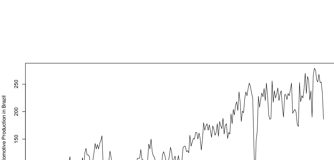
The automotive industry is extremely important as it can influence other industries activities. For example, 50% of the world rubber production, 25% of the world glass production and 15% of the world iron production are destined to the automotive industry. The behaviour of the data along time depicted in Figure 1 seems to indicate that an extra term should be included to take into account a (possibly nonlinear) trend. The term $\beta_{{\exp}}=\log(t)$ was then included in the model equation to account for this long-term increase.

The results regarding selection criteria are summarized in Table 4. We note that the three criteria indicate that the most appropriate model was the GARMA(1,1) Negative Binomial. Also, Table 5 presents the estimation results for the selected GARMA(1,1) Negative Binomial model with the extra parameter fixed at $k=150$.

We also performed a residual analysis based on the so called quantile residuals which are the common choice for generalized linear models. In fact, quantile residuals are the only useful residuals for binomial, negative binomial or Poisson data when the response takes on only a small number of distinct values ([Dunn and Smyth 1996]). These are given by $r_{t}=\Phi^{-1}(\textbf{F}_{y_{t}}(y_{t}|F_{t-1}))$ where $\textbf{F}_{y_{t}}$ represent the cumulative distribution function of the associated discrete distribution. In practice, when dealing with discrete distributions we need to introduce some randomization to produce continuous normal residuals. The residual analysis summarized in Figure 2 which indicates that the residuals are non-correlated and Gaussian distributed with mean 0.0767 and standard deviation 1.2295. Kolmogorov-Smirnov and Lilliefors normality tests returned $p$-values of 0.4502 and 0.0743 respectively which provides evidence for Gaussian assumption ([Conover 1999]).

Finally, we performed a prediction exercise using the last 9 observations of the original series as follows. For each $k=1,\dots,9$ the GARMA(1,1) negative binomial model was fitted to the series $y_{1},\dots,y_{n-k}$ and an out-of-sample one-step ahead prediction $\hat{y}_{n-k+1}$ was produced. These predictions can then be compared with the true values. The results are illustrated in Figure 3 from which we can see that the prediction errors are overall small. A formal comparison was made by calculating the mean absolute percentage error (MAPE, [Hyndman 2006]) and we obtained the value $6.07\%$.

This real data set comprises the number of hospitalizations caused by Dengue Fever in Campina Grande city (Brazil) between January 1998 and October 2003. Dengue Fever is transmitted by several species of mosquito within the $genusAedes$, principally A. aegypti. The Aedes mosquito is easily identifiable by the distinctive black and white stripes on its body. It prefers to lay eggs on clean and stagnant water. Analysing the autocorrelation function of this data, a seasonal behaviour is characterised. This is because the Summer months in this region present higher volume of rain, thus leading to more clean and stagnant water. Therefore we included two seasonal components in the model, $\beta_{{S}_{1}}$ and $\beta_{{S}_{2}}$, using cosine and sine functions respectively, and also considering the period of 12 months. These components are expected to improve model estimation.

The results regarding the selection criteria are summarized in Table 6 from which we can conclude that the most appropriate model was the GARMA(1,2) Negative Binomial. Note that the three criteria gave the same indication. Table 7 shows the estimation results for the selected GARMA(1,2) Negative Binomial model with the extra parameter fixed at $k=30$.

Again we performed a residual analysis based on quantile residuals. This is summarized in Figure 5 which indicates that the residuals are non-correlated and Gaussian distributed with mean 0.0258 and standard deviation 1.5571. The Kolmogorov-Smirnov and Shapiro-Wilk normality tests returned $p$-values of 0.4856 and 0.1176 respectively thus giving evidence for the Gaussian assumption.

A similar prediction exercise was performed for this data. So, we fitted a GARMA(1,2) negative binomial model to $y_{1},\dots,y_{n-k}$ and computed an out-of-sample one-step ahead prediction $\hat{y}_{n-k+1}$ for $k=1,\dots,9$. Figure 6 shows the predictions, prediction intervals and the real observations for comparison. It can be seen that, although relatively close to the actual values, predictions for May, June, July and August 2003 are consistently below the observations. The MAPE criterion was calculated as $47.81\%$.

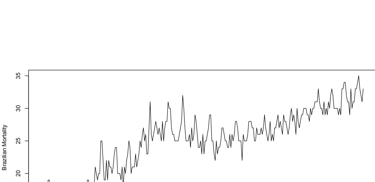
Our last real data set is the number of deaths in Brazil between January 1984 and December 2007. This data is available from the Brazilian Health Ministry at http://www2.datasus.gov.br/DATASUS and is depicted in Figure 7. Likewise the first example, the original series was divided by 1000 to reduce the magnitude of the data. As in the first example, we think there is a point for the inclusion of an extra term here too since the series exhibits a long-term (possibly nonlinear) increase. So, a new component $\beta_{{\exp}}=\log(t)$ was added to the model equation as this is expected to improve model estimation.

Looking at the Bayesian selection criteria given in Table 8 we can conclude that the best model for this particular data is the GARMA(1,0) Binomial model. There are only three parameters in this model and the estimation results are shown in Table 9. Here the extra parameter was fixed at $m=45$.

The residual analysis summarized in Figure 8 indicates that the residuals are non-correlated and Gaussian distributed with mean 0.1850 and standard deviation 0.4894. The Kolmogorov-Smirnov and Anderson-Darling normality tests returned $p$-values of 0.6736 and 0.1304 respectively thus indicating evidence for the Gaussian assumption.

Likewise the previous examples we repeated the prediction exercise here. This time we used the 10 last observations as the series is longer. So, the GARMA(1,0) binomial model was fitted to the series $y_{1},\dots,y_{n-k}$ and a one-step ahead prediction $\hat{y}_{n-k+1}$ was produced for $k=1,\dots,10$. The results are illustrated in Figure 9 from which we can see that the prediction errors are again overall small. Using these prediction errors the calculated value for the MAPE criterion was $3.63\%$.

References

- Benjamin, Rigby, and Stasinopoulos 2003 Benjamin, M. A., R. A. Rigby, and D. M. Stasinopoulos (2003). Generalized autoregressive moving average models. J. Amer. Statist. Assoc. 98, 214–223.
- Biswas and Song 2009 Biswas, A. and P. X.-K. Song (2009). Discrete-valued ARMA processes. Statistics and Probability Letters 79(17), 1884–1889.
- Carlin and Louis 2001 Carlin, B. P. and T. A. Louis (2001). Bayes and Empirical Bayes methods for data analysis. Boca Raton: Chapman and Hall/CRC.
- Chan and Ledolter 1995 Chan, K. and J. Ledolter (1995). Monte Carlo E.M. estimation for time series models involving counts. Journal of the American Statistical Association 90, 242–251.
- Chen and Shao 1998 Chen, M. and Q. Shao (1998). Monte Carlo estimation of Bayesian credible and HPD intervals. Journal of Computational and Graphical Statistics 8, 69–92.
- Conover 1999 Conover, W. J. (1999). Practical Nonparametric Statistics (3rd ed.). Wiley series in Probability and Statistics. New York: Wiley.
- Davis, Dunsmuir, and Streett 2003 Davis, R. A., W. T. Dunsmuir, and S. B. Streett (2003). Observation-driven models for Poisson counts. Biometrika 90(4), 777–790.
- Davis, Dunsmuir, and Wang 1999 Davis, R. A., W. T. Dunsmuir, and Y. Wang (1999). Modelling time series of counts data. Asymptotic, Nonparametric, and Time Series Ed. S. Ghosh, 63–114.
- Dunn and Smyth 1996 Dunn, P. K. and G. K. Smyth (1996). Randomized quantile residuals. Journal of Computational and Graphical Statistics 5, 236–244.
- Gelfand, Dey, and Chang 1992 Gelfand, A. E., D. K. Dey, and H. Chang (1992). Model determination using predictive distributions with implementation via sampling-based methods. Bayesian Statistics 4, 147–167.
- Geweke 1992 Geweke, J. (1992). Evaluating the accuracy of sampling-based approaches to the calculation of posterior moments. In Bayesian Statistics 4, 169–193.
- Hyndman 2006 Hyndman, R. J. (2006). Another look at measures of forecast accuracy. International Journal of Forecasting 22(4), 679–688.
- Jung, Kukuk, and Liesenfeld 2006 Jung, R. C., M. Kukuk, and R. Liesenfeld (2006). Time series of count data: Modeling, estimation and diagnostics. Comput. Stat. Data Anal 51, 2350–2364.
- Liesenfeld, Nolte, and Pohlmeier 2006 Liesenfeld, R., I. Nolte, and W. Pohlmeier (2006). Modelling financial transaction price moviments: a dynamic integer count data model. Empirical Econom. 30, 795–825.
- McCullagh and Nelder 1989 McCullagh, P. and J. A. Nelder (1989). Generalized Linear Models. Chapman and Hall, London, 2nd. Edition.
- R Development Core Team 2010 R Development Core Team (2010). R: A language and environment for statistical computing. Vienna, Austria: R Foundation for Statistical Computing.
- Rydberg and Shephard 2003 Rydberg, T. and N. Shephard (2003). Dynamics of trade-by-trade price movements: decomposition and models. Journal of Finan. Econom. 1, 2–25.
- Spiegelhalter, Best, Carlin, and Van der Linde 2002 Spiegelhalter, D. J., N. G. Best, B. P. Carlin, and A. Van der Linde (2002). Bayesian mensures of model complexity and fit. Journal of the Royal Statistical Society: Series B 64(4), 583–639.
- Zeger 1988 Zeger, S. L. (1988). A regression model for time series of counts. Biometrika 75(4), 621–629.
- Zhu 2010 Zhu, F. (2010). A negative binomial integer-valued GARCH model. Journal of Time Series Analysis 32, 54–67.