Interior of Black Holes and Information Recovery

Hikaru Kawai Note: hkawai@gauge.scphys.kyoto-u.ac.jp Affiliation: Department of Physics, Kyoto University, Kyoto 606-8502, Japan Yuki Yokokura Note: yuki.yokokura@icts.res.in Affiliation: International Centre for Theoretical Sciences, Survey No.151, Shivakote, Hesaraghatta Hobli, Bengaluru North - 560 089, India.

Abstract

We analyze time evolution of a spherically symmetric collapsing matter from a point of view that black holes evaporate by nature. We first consider a spherical thin shell that falls in the metric of an evaporating Schwarzschild black hole of which the radius $a(t)$ decreases in time. The important point is that the shell can never reach $a(t)$ but it approaches $a(t)-a(t)\frac{\mathrm{d}a(t)}{\mathrm{d}t}$ . This situation holds at any radius because the motion of a shell in a spherically symmetric system is not affected by the outside. In this way, we find that the collapsing matter evaporates without forming a horizon. Nevertheless, a Hawking-like radiation is created in the metric, and the object looks the same as a conventional black hole from the outside. We then discuss how the information of the matter is recovered. We also consider a black hole that is adiabatically grown in the heat bath and obtain the interior metric. We show that it is the self-consistent solution of $G_{\mu\nu}=8\pi G\langle T_{\mu\nu}\rangle$ and that the four-dimensional Weyl anomaly induces the radiation and a strong angular pressure. Finally, we analyze the internal structures of the charged and the slowly rotating black holes.

pacs

04.62.+v, 04.70.Dy, 11.10.-z.

I Introduction

The picture of the black hole has changed significantly since the discovery of the Schwarzschild solution. In the classical level black holes are characterized by the existence of the event horizon, and objects which have entered into them cannot come back forever. In the quantum level, however, black holes evaporate in the vacuum [1] and can be in equilibrium with the heat bath of the Hawking temperature [2]. One of the problems of this picture is the information paradox [3], which is essentially the disagreement between the information flow and the energy flow. Suppose we consider a process in which a black hole is formed by the collapse of matter. In the conventional picture, the matter crosses the horizon holding its own information. On the other hand, the Hawking radiation is thermal because it is created in vacuum, and it cannot reflect the detailed information of the collapsing matter. Therefore, if we assume that the evaporation occurs after the horizon is formed, we are forced to conclude that, although all the energy is emitted to infinity, the fallen information does not come back. In this paper, we reconsider the time evolution of the collapsing matter from the point of view that black holes are objects that evaporate inherently. Then, we find that no horizon appears and the matter is distributed in the whole region inside the black hole. Furthermore, we discuss that the Hawking radiation comes out through the matter and can exchange information with it.

In order to understand the absence of the horizon, we first consider a spherical shell falling in the evaporating Schwarzschild metric. The important point is that the radius $a(t)$ is decreasing as $\frac{\mathrm{d}a(t)}{\mathrm{d}t}=-\frac{Cl_{p}^{2}}{a(t)^{2}}$ due to the Hawking radiation. Here $a=2GM$ is the Schwarzschild radius, $l_{p}=\sqrt{\hbar G}$ is the Planck length, and $C$ is a proportionality constant of order $\mathcal{O}(1)$ . Then, the shell does not catch up with the horizon completely but approaches to $r=a(t)+\frac{Cl_{p}^{2}}{a(t)}$ . This is because the shell approaches the horizon in the time scale $a$ , but during that time the radius $a$ decreases by $\Delta a=\left|\frac{\mathrm{d}a}{\mathrm{d}t}\right|a=\frac{Cl_{p}^{2}}{a}$ .

We then consider a spherically symmetric collapsing matter with a continuous distribution, and regard it as a set of thin shells. Because of the spherical symmetry the time evolution of each shell is not affected by the shells outside it. Then, the above argument can be applied to each shell. Thus, there is no trapped region, and no horizon appears. Nevertheless, we can show that a radiation is created from each shell, and it takes almost the same form as the conventional Hawking radiation. Interestingly, a strong angular pressure is also induced, against which the shell collapses and loses the energy.

From these discussions it turns out that the evaporating object has a clear surface at $r=a(t)+\frac{Cl_{p}^{2}}{a(t)}$ and that its interior is filled with matter and radiation while from the outside it looks almost the same as the conventional black hole. As we will see, no trans-Planckian problems occur if the theory has many fields, for example about 100.

This picture of black holes indicates possible mechanisms of the information recovery. Since the Hawking radiation is produced near each shell, the radiation and the collapsing matter can interact and exchange the detailed information. The time scale of this process can be estimated as $\sim a\log\frac{a}{l_{p}}$ . Based on this mechanism, we discuss the possibility that the radiation depends on the initial information of the collapsing mater.

We also discuss a black hole which is adiabatically grown in the heat bath. We obtain its interior metric and show that it is the self-consistent solution of the semiclassical Einstein equation $G_{\mu\nu}=8\pi G\langle T_{\mu\nu}\rangle$ . Then, it is understood that the the four-dimensional Weyl anomaly produces the radiation and the angular pressure. We can also investigate the interior structure of the charged and the slowly rotating black holes.

This paper is organized as follows. In Sec. II, we explain the new picture of black holes. In Sec. III, we discuss how the information comes back in the process of evaporation, and consider possible mechanisms of information recovery. In Sec. IV, we consider the black hole that is adiabatically grown in the heat bath. In Secs. V and VI, we study the charged and the slowly rotating black holes. We give supplementary discussions in the Appendixes.

II New picture of black holes

II.1 Conventional picture of black holes

We review here the conventional picture of black holes. Suppose we consider a Schwarzschild black hole in the vacuum with a large mass $M=\frac{a}{2G}$ compared with the Planck mass $m_{p}\equiv\sqrt{\frac{\hbar}{G}}$ . The black hole has the Hawking temperature and the Bekenstein-Hawking entropy [1, 2, 4],

T_{H}=\frac{\hbar}{4\pi a},~~~S_{BH}=\frac{A}{4l_{p}^{2}}~,

(1)

where $A=4\pi a^{2}$ is the area of the horizon. From the Stephan-Boltzmann law [5], the time evolution of $a(t)$ can be expressed as

\frac{\mathrm{d}a}{\mathrm{d}t}=-\frac{2\sigma(a)}{a^{2}}~.

(2)

Here $\sigma(a)$ is $l_{p}^{2}$ multiplied by a constant of order 1. $\sigma(a)$ depends on the detail of the theory, such as the number of species of fields [6]. We expect that $\sigma(a)$ varies with $a$ slowly compared with $l_{p}$ ; $\frac{\mathrm{d}\sigma}{\mathrm{d}a}l_{p}\ll\sigma$ . Although these results were originally obtained by assuming the existence of the horizon, as we will see later, collapsing matter radiates and has the same entropy even if there is no horizon.

Next we consider the smallest unit of energy following Bekenstein’s argument [4]. Suppose we inject a wave packet of a massless particle with energy $\epsilon$ to a black hole with radius $a$ . In order for the wave to enter into the black hole, its wavelength needs to be smaller than the size of the black hole:

\lambda\lesssim a.

(3)

Therefore, its energy should satisfy

\epsilon=\hbar\omega=\hbar\frac{2\pi}{\lambda}\gtrsim\frac{\hbar}{a}.

(4)

Thus, the minimum energy that can be added to a black hole with radius $a$ is given by

\epsilon\sim\frac{\hbar}{a}~,

(5)

and the corresponding wavelength is

\lambda\sim a~.

(6)

Although the above argument is valid for massless particles, we can show the same results also for massive particles (see Appendix A).

The minimum energy 5 corresponds to 1 bit of information, because the wavelength of the particle 6 is as large as the black hole, and we have two possibilities, whether it goes inside the hole or not. Now, suppose we build up a black hole with radius $a$ from particles which have the minimum energy. Then, the total amount of the lost information is evaluated as

	$\displaystyle S$	$\displaystyle\sim{\rm(the~number~of~processes)}\times{\rm(entropy~per~a~process)}$
		$\displaystyle\sim\frac{a}{G\epsilon}\times\log 2\sim\frac{a^{2}}{l_{p}^{2}}~,$		(7)

which agrees with $S_{BH}$ in 1. Note that if we use particles with $\epsilon\gg\frac{\hbar}{a}$ the entropy is much less than 7 (see Appendix A). As we will see later, the existence of the horizon is not essential for this estimation.

II.2 Motion of a test particle near the evaporating black hole

We analyze here the motion of a test particle near the evaporating Schwarzschild black hole. The outside spacetime can be approximately described by

\mathrm{d}s^{2}=-\frac{r-a(t)}{r}\mathrm{d}t^{2}+\frac{r}{r-a(t)}\mathrm{d}r^{2}+r^{2}\mathrm{d}\Omega^{2}~,

(8)

where $a(t)$ satisfies 2 [7]. If the test particle comes sufficiently close to $a(t)$ , its radial coordinate $r(t)$ is determined irrespectively of its mass or angular momentum by

\frac{\mathrm{d}r(t)}{\mathrm{d}t}=-\frac{r(t)-a(t)}{r(t)}~.

(9)

This is because any particle becomes ultrarelativistic near $r\sim a$ and behaves like a massless particle [10] [11]. From 9 we see that the particle approaches the radius $a$ in the time scale of $\mathcal{O}(a)$ . During this time, however, the radius $a(t)$ itself is slowly shrinking due to the Hawking radiation. Hence, the particle cannot catch up with the radius $a$ completely. Instead, $r(t)$ is always apart from $a(t)$ by $-a\frac{\mathrm{d}a}{\mathrm{d}t}$ . See Fig.1.

Refer to caption — Figure 1: A test particle in the time-dependent Schwarzschild metric. $r(t)$ cannot catch up with $a(t)$ as long as $\frac{\mathrm{d}a}{\mathrm{d}t}(t)<0$ .

We can see this behavior explicitly by solving 9 as follows. Putting $r(t)=a(t)+\Delta r(t)$ in 9 and assuming $\Delta r(t)\ll a(t)$ , we have

\frac{\mathrm{d}\Delta r(t)}{\mathrm{d}t}=-\frac{\Delta r(t)}{a(t)}-\frac{\mathrm{d}a(t)}{\mathrm{d}t}~.

(10)

The general solution of this equation is given by

\Delta r(t)=C_{0}e^{-\int^{t}_{t_{0}}\mathrm{d}t^{\prime}\frac{1}{a(t^{\prime})}}+\int^{t}_{t_{0}}\mathrm{d}t^{\prime}\left(-\frac{\mathrm{d}a}{\mathrm{d}t}(t^{\prime})\right)e^{-\int^{t}_{t^{\prime}}\mathrm{d}t^{\prime\prime}\frac{1}{a(t^{\prime\prime})}},

where $C_{0}$ is an integration constant. Because $a(t)$ and $\frac{\mathrm{d}a}{\mathrm{d}t}(t)$ can be considered to be constant in the time scale of ${\cal O}(a)$ , the second term can be evaluated as

		$\displaystyle\int^{t}_{t_{0}}\mathrm{d}t^{\prime}\left(-\frac{\mathrm{d}a}{\mathrm{d}t}(t^{\prime})\right)e^{-\int^{t}_{t^{\prime}}\mathrm{d}t^{\prime\prime}\frac{1}{a(t^{\prime\prime})}}$
		$\displaystyle\approx-\frac{\mathrm{d}a}{\mathrm{d}t}(t)\int^{t}_{t_{0}}\mathrm{d}t^{\prime}e^{-\frac{t-t^{\prime}}{a(t)}}=-\frac{\mathrm{d}a}{\mathrm{d}t}(t)a(t)(1-e^{-\frac{t-t_{0}}{a(t)}}).$

Therefore we obtain

\Delta r(t)\approx C_{0}e^{-\frac{t-t_{0}}{a(t)}}-\frac{\mathrm{d}a}{\mathrm{d}t}(t)a(t)(1-e^{-\frac{t-t_{0}}{a(t)}}),

which leads to

	$\displaystyle r(t)$	$\displaystyle\approx a-a\frac{\mathrm{d}a}{\mathrm{d}t}+Ce^{-\frac{t}{a}}$
		$\displaystyle=a+\frac{2\sigma(a)}{a}+Ce^{-\frac{t}{a}}\longrightarrow a+\frac{2\sigma}{a}~,$		(11)

where $C$ is a positive constant and we have used 2 to obtain the second line. This result indicates that in the time scale of ${\cal O}(a)$ any particle approaches

R(a)\equiv a+\frac{2\sigma(a)}{a}~,

(12)

and it will never cross the radius $a(t)$ as long as $a(t)$ keeps decreasing. In the following we call $R(a)$ the surface of the black hole. We give a numerical demonstration of 11 in Appendix B.

One might wonder if such a small radial difference $\frac{2\sigma}{a}$ makes sense, since it looks much smaller than $l_{p}$ . However, the proper distance between the surface and the horizon is estimated as

\Delta l=\sqrt{g_{rr}(R(a))}\frac{2\sigma(a)}{a}\approx\sqrt{2\sigma(a)}~,

(13)

because $g_{rr}(r)=\frac{r}{r-a}$ . In general this is proportional to $l_{p}$ , but the coefficient can be large if we consider a theory with many species of fields. In fact, in that case we have

\sigma\sim Nl_{p}^{2}\gg l_{p}^{2}~,

(14)

where $N$ is the number of fields. We assume that $N$ is large but not infinite, for example, of the order of 100 as in the standard model.

So far, we have found the surface 12 based on the classical motion of particles. However, we can show that the result is valid even if we treat the particles quantum mechanically. Suppose that we throw a wave packet of a massless particle with frequency $\omega$ to the black hole [12]. Here, $\omega$ is measured at $r\gg a$ and there the wavelength is given by $\lambda=\frac{2\pi}{\omega}$ . Then, it becomes blueshifted as it approaches to $r=a+\Delta r$ :

\omega_{local}=\frac{\omega}{\sqrt{-g_{tt}(r)}}~.

Thus, the local wavelength is given by

\lambda_{local}=\frac{2\pi}{\omega_{local}}=\sqrt{-g_{tt}(r)}\lambda\approx\sqrt{\frac{\Delta r}{a}}\lambda~.

On the other hand, the proper distance $l$ from $r=a$ is given by

	$\displaystyle l$	$\displaystyle=\int^{\Delta r+a}_{a}\mathrm{d}r\sqrt{g_{rr}}=\int^{\Delta r+a}_{a}\mathrm{d}r\frac{1}{\sqrt{1-\frac{a}{r}}}$
		$\displaystyle\approx\int^{\Delta r+a}_{a}\mathrm{d}r\sqrt{\frac{a}{r-a}}=2\sqrt{a\Delta r}~.$		(15)

Therefore, in order that the wave is contained in a region with the size $l$ , the wavelength needs to satisfy

1\lesssim\frac{l}{\lambda_{local}}=\frac{2a}{\lambda}~,

(16)

which turns out to be the same as 3. This tells that such a wave packet that can go into the black hole behaves as a particle near $r=a$ . Therefore, we can conclude that 12 is the position where any wave approaches. Note that 16 is nothing but the condition for the eikonal approximation.

II.3 New picture

II.3.1 Surface of black holes

We consider spherically symmetric collapsing matter that forms a black hole in the conventional picture. As is discussed in Appendix C, we can regard it as consisting of thin shells with the minimum energy 5. An important point is that because of the spherical symmetry, the time evolution of each shell is not affected by the shells outside it, if we describe the motion using the local time. Then, assuming that the mass inside each shell is decreasing as in 2, we can apply 12 for each shell, and find that it is always apart from its Schwarzschild radius. Therefore, we can conclude that there is no trapped region.

Next, we consider the outermost shell. Because its radius approaches $R(a(t))=a(t)+\frac{2\sigma(a(t))}{a(t)}$ , all matter is stuffed in the region $r<R(a(t))$ , which means that the object has a clear boundary at $r=R(a(t))$ . This is the reason why we call $R(a)$ the surface [13]. The region outside the surface is almost empty, and the object looks exactly the same as the conventional black holes when it is observed from the outside. On the other hand, the inside of the surface is totally different. In particular, the horizon no longer exists [8, 15, 16] because of the nontrivial distance 13. In the following, we call the object a black hole, although it is significantly different from the conventional ones.

Here, one might wonder if the Hawking radiation is really created by such an object. However, we can show that indeed it is [8, 15] (see also Appendix C). Generally, particle creation occurs in a time-dependent potential, and it takes the Planck-like distribution if the affine parameters on the null generators of the past and future null infinity are related exponentially [17]. Indeed, in Appendix D, using the self-consistent metric obtained in Sec. IV, we show that particles are created from the vacuum in accordance with the Planck-like distribution with the Hawking temperature [18]

T_{H}(t)=\frac{\hbar}{4\pi a(t)}~.

(17)

However, as we will see in Sec. II.4, the distribution may be modified by the interaction between the collapsing matter and the radiation.

II.3.2 Self-consistent time evolution of each shell

In this subsection we investigate how each shell loses energy during the Hawking radiation. When we analyze the time evolution of a shell, we can ignore the matter outside it because of the spherical symmetry, and regard the system as consisting of the shell and the core. Here, the core is the part of the system inside the shell, and we denote its radius and mass by $r^{\prime}$ and $\frac{a^{\prime}}{2G}$ , respectively. For simplicity, we assume that $r^{\prime}$ is already very close to $R(a^{\prime})$ and that the Hawking radiation is emitted as a conventional black hole,

\frac{\mathrm{d}a^{\prime}}{\mathrm{d}t^{\prime}}=-\frac{2\sigma(a^{\prime})}{a^{\prime 2}}~,

(18)

where $t^{\prime}$ is the time without taking the matter outside the core into account. We also assume for simplicity that the shell has no thickness and denote its radius by $r_{s}$ .

Now we can discuss how the energy of the shell decreases from its initial value, which we assume to be $\epsilon\sim\frac{\hbar}{a}$ . We can consider the following three stages. See Fig.2.

Stage I.—The shell is far from the core, and the radiation emitted from the core is not altered by the shell. The total mass $\frac{a(t)}{2G}$ decreases as

\frac{\mathrm{d}a}{\mathrm{d}t}\approx-\frac{2\sigma(a^{\prime})}{a^{\prime 2}}~.

(19)

Stage II.—In the time scale of order $a$ , the shell comes close to the core. Then the total system behaves like a black hole with radius $a$ , the surface of which is located at $r=r_{s}=R(a)$ , and radiates as usual 2. However, the radiation comes mainly from the shell because the radiation from the core is extremely weakened by the redshift $\frac{\mathrm{d}t}{\mathrm{d}t^{\prime}}$ caused by the shell, although the core itself radiates constantly as 18 in terms of $t^{\prime}$ . Therefore, $a^{\prime}(t)$ , and thus $R(a^{\prime}(t))$ , change very little during this stage.

We can examine the time evolution of the energy of the shell more precisely, which is given by $\epsilon(t)=\frac{\Delta a(t)}{2G}$ , where $\Delta a=a-a^{\prime}$ . The metric outside the core is given by

\mathrm{d}s^{2}=\begin{cases}-\frac{r-a(t)}{r}\mathrm{d}t^{2}+\frac{r}{r-a(t)}\mathrm{d}r^{2}+r^{2}\mathrm{d}\Omega^{2},~~~~~{\rm for}~r_{s}\leq r,\\ -\frac{r-a^{\prime}(t^{\prime})}{r}\mathrm{d}t^{\prime 2}+\frac{r}{r-a^{\prime}(t^{\prime})}\mathrm{d}r^{2}+r^{2}\mathrm{d}\Omega^{2},~{\rm for}~R(a^{\prime})\leq r\leq r_{s},\end{cases}

(20)

where $a(t)$ and $a^{\prime}(t^{\prime})$ follow 2 and 18, respectively. The relation between $t$ and $t^{\prime}$ is obtained as follows. First, we write the time evolution of $r_{s}$ in two ways using the metric outside and inside the shell:

\frac{\mathrm{d}r_{s}}{\mathrm{d}t}=-\frac{r_{s}(t)-a(t)}{r_{s}(t)},~~~\frac{\mathrm{d}r_{s}}{\mathrm{d}t^{\prime}}=-\frac{r_{s}(t^{\prime})-a^{\prime}(t^{\prime})}{r_{s}(t^{\prime})}~.

(21)

Then, by taking the ratio, we get

	$\displaystyle\frac{\mathrm{d}t^{\prime}}{\mathrm{d}t}$	$\displaystyle=\frac{r_{s}-a}{r_{s}-a^{\prime}}=\frac{\frac{2\sigma(a)}{a}}{\frac{2\sigma(a)}{a}+\Delta a}$		(22)
		$\displaystyle\approx 1-\frac{a\Delta a}{2\sigma(a)}$		(23)

where we have used $r_{s}=R(a)=a+\frac{2\sigma(a)}{a}$ and assumed $\Delta a\lesssim\frac{l_{p}^{2}}{a}$ together with 14. By using 2, 18, 23, and $\frac{1}{a^{\prime 2}}\approx\frac{1}{a^{2}}\left(1+\frac{2\Delta a}{a}\right)$ , we obtain

$\displaystyle\frac{\mathrm{d}\epsilon}{\mathrm{d}t}$	$\displaystyle=\frac{1}{2G}\left(\frac{\mathrm{d}a}{\mathrm{d}t}-\frac{\mathrm{d}a^{\prime}}{\mathrm{d}t}\right)=\frac{1}{2G}\left(\frac{\mathrm{d}a}{\mathrm{d}t}-\frac{\mathrm{d}t^{\prime}}{\mathrm{d}t}\frac{\mathrm{d}a^{\prime}}{\mathrm{d}t^{\prime}}\right)$
	$\displaystyle\approx-\frac{1}{2G}\left[\frac{2\sigma(a)}{a^{2}}-\left(1-\frac{a\Delta a}{2\sigma(a)}\right)\frac{2\sigma(a)}{a^{2}}\left(1+\frac{2\Delta a}{a}\right)\right]$
	$\displaystyle\approx-\frac{\epsilon}{a}~,$	(24)

which gives

\epsilon(t)=\epsilon(0)e^{-\frac{t}{a(t)}}~.

(25)

Here we have used the fact that $a(t)$ does not change significantly in the time scale of $\mathcal{O}(a)$ . Thus, the energy of the shell decreases exponentially in the time scale

\Delta t_{decay}\sim a~.

(26)

Note that the redshift 23 plays a crucial role in 24. This indicates that in general the radiation observed from the outside comes from the region near the surface.

Stage III.—When the energy of the shell is exhausted, the core starts to radiate without redshift.

Because the above argument can be applied to any shell, we conclude that the whole object evaporates from the outside as if an onion is peeled. A more detailed analysis is as follows. First we estimate how many shells around the surface are moving without large redshift. From 22, we have

\frac{\mathrm{d}t^{\prime}}{\mathrm{d}t}=\mathcal{O}(1)\lesssim 1\Longleftrightarrow\Delta a\lesssim\frac{\sigma}{a}~.

(27)

Therefore, if we consider a black-hole-like object with radius $a_{0}$ , the outermost region with the width

\Delta r_{surface}\sim\frac{\sigma(a_{0})}{a_{0}}

(28)

is not frozen, which contains $\frac{\sigma}{l_{p}^{2}}$ shells with energy $\epsilon\sim\frac{\hbar}{a_{0}}$ . Then, the lifetime of the object is estimated as

$\displaystyle\Delta t_{life}$	$\displaystyle\sim({\rm the~decay~time~of~a~shell})$
	$\displaystyle~~\times\frac{({\rm the~total~number~of~the~shells})}{({\rm the~number~of~shells~moving~at~the~same~time})}$
	$\displaystyle\sim a_{0}\times\left(\frac{\frac{a_{0}}{G}}{\epsilon}\times\frac{1}{\frac{\sigma}{l_{p}^{2}}}\right)\sim\frac{a_{0}^{3}}{\sigma}~,$	(29)

which agrees with the one obtained from 2.

II.3.3 Interior of the evaporating black hole

Now we consider the interior of the object. See Fig.3.

We examine the region deeper than the outermost one considered in the previous subsection. In terms of the local time, the shells in this region simply keep falling as 9 for the local quantities $r^{\prime}$ , $a^{\prime}$ , and $t^{\prime}$ (see the lower closeup of Fig.3). However, if we see them from the outside, time is frozen due to the large redshift after the outermost shells come close to the surface. To check this explicitly, we consider a shell with radius $r^{\prime}$ in the deep region so that $\Delta a=a-a^{\prime}\gg\Delta r_{surface}\sim\frac{\sigma}{a}$ . Here, $a$ and $a^{\prime}$ are the Schwarzschild radius corresponding to the mass of the total system and that inside the shell, respectively. An important point here is that the shell has not necessarily reached $R(a^{\prime})$ . In fact, in that case, Eq. 22 becomes

\frac{\mathrm{d}t^{\prime}}{\mathrm{d}t}\approx\frac{2\sigma}{a\Delta a}~,

(30)

which leads to

\Delta t^{\prime}\sim a\Longleftrightarrow\Delta t\sim\frac{a^{2}}{\sigma}\Delta a\gg a~.

(31)

As we have seen, $\Delta t^{\prime}\sim a$ is the time scale in which the shell reaches $R(a^{\prime})$ . On the other hand, $\Delta t\sim\frac{a^{2}}{\sigma}\Delta a$ is the time scale in which the matter outside the shell evaporates by the Hawking radiation. Thus, we have seen that the interior region is almost frozen and its structure depends on the initial distribution [19]. Each shell starts to evolve after the matter outside it disappears.

Next, we discuss the outermost region with the width $\sim\frac{\sigma}{a}$ , where time flows without large redshift. For any initial distribution, each shell in this region reaches the asymptotic position $R(a^{\prime})$ in the time scale $a$ . Then, the Hawking radiation starts to be created, and the energy of the shell decreases exponentially as 25 (see the upper closeup of Fig.3). As we will see later, this time evolution depends on the initial data, which gives a natural mechanism of the information recovery.

So far, we have found that a collapsing matter becomes a compact object with the surface located at $r=R(a(t))$ , and it evaporates without forming a trapped region in the time scale of $\frac{a^{3}}{\sigma}$ . We will also see in Sec. II.6 that no trans-Planckian problem occurs if the theory has many species of matter fields. Thus, we obtain the Penrose diagram as in Fig.4, which is topologically the same as the Minkowski space [8, 15] [20].

II.4 Closer look at the surface and intensity $\sigma(a)$

In this subsection we examine the surface more precisely. In particular, we consider the effect that some portion of the Hawking radiation is scattered back due to the gravitational potential or scattering with the other matters.

The outermost region is magnified in Fig.5. Here, for simplicity, time is discretized to the interval $\Delta t\sim a$ . $S$ stands for the surface which is located at $r=R(a(t))=a(t)+\frac{2\sigma(a(t))}{a(t)}$ . Suppose that matter or radiation with energy $\epsilon\sim\frac{\sigma_{0}(a)}{a}$ is emitted from the surface at $t=t_{i}$ , which is shown as $P_{i}$ in the figure [23]. Here $\sigma_{0}(a)$ is the “raw intensity” before taking the scattered flow into account. In the time scale $a$ , the matter reaches $r=r_{g}\equiv a+\Delta r$ , where $\Delta r\sim a$ . At this point $Q_{i+1}$ , some amount of the matter is scattered back while the rest goes to infinity. In order to indicate the portion of the scattered energy, $\epsilon_{scat}$ , we introduce a function $g(a)$ as

\epsilon_{scat}=\frac{g(a)}{1+g(a)}\epsilon~.

(32)

$g(a)$ should be an order 1 quantity and may depend on the matter Lagrangian. Then, in the time scale $a$ , the scattered matter comes back to the surface $S$ , which is shown as $P_{i+2}$ . Then, it enters into the object and keeps going along the trajectory $S_{i+2}$ , and it is covered by the subsequent matter or radiation. Here, $S_{i}$ is located at $r=R_{0}(a_{i})\equiv a_{i}+\frac{2\sigma_{0}(a_{i})}{a_{i}}$ , which is the asymptotic position of the shell that started from $Q_{i-1}$ . Thus, a part of the Hawking radiation comes back in the time scale $\sim a$ . This process occurs continuously, and we find that the physical surface $S$ consists of the scattered matter and radiation.

Now, we relate the raw intensity $\sigma_{0}$ to the net intensity $\sigma$ . To do it, we estimate how the mass of the total system decreases during $t_{i+2}\leq t\leq t_{i+3}$ . Adding the decrease by the raw emission and the increase by the scattered energy 32, we have

	$\displaystyle\Delta a$	$\displaystyle=-\frac{2\sigma_{0}}{a_{i+2}^{2}}\Delta t+\frac{g}{1+g}\frac{2\sigma_{0}}{a_{i}^{2}}\Delta t$
		$\displaystyle\approx-\frac{2\sigma_{0}}{a^{2}}\Delta t+\frac{g}{1+g}\frac{2\sigma_{0}}{a^{2}}\Delta t=-\frac{1}{1+g}\frac{2\sigma_{0}}{a^{2}}\Delta t~.$		(33)

Comparing this with 2, we obtain

\sigma(a)\equiv\frac{\sigma_{0}(a)}{1+g(a)}~.

(34)

Although $g(a)$ may depend on the detail of the matter Lagrangian, the argument in Sec. II.2 is still valid, and the position of the surface $S$ is determined by $\sigma$ , as in 12.

II.5 Stationary black holes in the heat bath

Here we consider how the black-hole-like object becomes in equilibrium with the heat bath. Suppose an evaporating object with mass $\frac{a}{2G}$ is put in the heat bath of temperature $T_{H}=\frac{\hbar}{4\pi a}$ . As the matter in the outermost region comes out of the object [23], the radiation from the heat bath replaces it. Because the collapsing matter is replaced by the radiation in the heat bath, this process is not an equilibrium one. After this process is completed in the outermost region, the system becomes stationary. Figure 6 represents this situation.

The remarkable point is that this process occurs only in the outermost region where time flows. The matter in the deeper region is almost frozen and keeps having its initial information. Nevertheless, the total object becomes in equilibrium with the heat bath in that the outgoing and ingoing flows balance almost completely. In the rigorous sense it is merely a stationary state, but in practice it behaves as an equilibrium state. Finally, we show the Penrose diagram. See Fig. 7.

While the interior structure depends on the initial distribution of matter, the exterior is universally described by the Schwarzschild metric, Eq. 8 with $a=$ const..

II.6 Absence of trans-Planckian problems

In this subsection we will show that the trans-Planckian effects are absent if the theory has many fields. We consider the matter in the outermost region with width $\sim\frac{\sigma}{a}$ , where time flows as is discussed in 28. The energy of the matter is given by $\epsilon\sim\frac{\sigma}{Ga}$ due to the relation $a=2GM$ . Because the energy of the minimum quantum is $\epsilon_{1}\sim\frac{\hbar}{a}$ as discussed by Bekenstein [4], we can regard the matter as consisting of $\frac{\epsilon}{\epsilon_{1}}\sim\frac{\sigma}{l_{p}^{2}}\sim N$ quanta. This is consistent with the fact that we have $N$ species of fields. In fact, we can consider how the $N$ quanta with wavelength $\sim a$ are compressed to form the outermost region just outside the core. See Fig. 8. During this process, the waves are adiabatically compressed because the initial wavelength is $\sim a$ , and the condition 16 is satisfied.

Each quantum with energy $\epsilon_{1}\sim\frac{\hbar}{a}$ is blueshifted as it falls toward the core, and the energy becomes

\epsilon_{1}^{local}=\frac{\epsilon_{1}}{\sqrt{-g_{tt}(R(a))}}\sim\frac{\hbar}{\sqrt{\sigma(a)}}~.

(35)

Here we have used 12 and 20 to obtain $g_{tt}(R(a))=-\frac{R(a)-a}{R(a)}\approx-\frac{2\sigma(a)}{a^{2}}$ . From 14, we have $\epsilon_{1}^{local}\ll m_{p}$ when $N$ is large. This indicates that each quantum does not have trans-Planckian energy.

It should be noted that the wavelength $\lambda^{local}_{1}$ of each quantum is of the same order as the proper length $\Delta l$ of the outermost region:

	$\displaystyle\lambda^{local}_{1}$	$\displaystyle=\frac{\hbar}{\epsilon_{1}^{local}}\sim\sqrt{\sigma(a)}$		(36)
	$\displaystyle\Delta l$	$\displaystyle\sim\sqrt{g_{rr}(R(a))}\frac{\sigma(a)}{a}\sim\sqrt{\sigma(a)}~.$		(37)

Here we have used 12 and 20 to obtain $g_{rr}(R(a))=\frac{R(a)}{R(a)-a}\approx\frac{a^{2}}{2\sigma(a)}$ . This gives another support to the picture that the waves are adiabatically compressed as in Fig. 8 [24].

The above results suggest that the typical scale in which things change is $\sim\sqrt{\sigma}$ . Therefore, the curvature can be estimated as

{\cal R}\sim\frac{1}{(\sqrt{\sigma})^{2}}\sim\frac{1}{\sigma}~,

(38)

which is smaller than $l_{p}^{-2}$ from 14. We will justify this result in Sec. IV by examining the self-consistent metric. See Eq. 75.

We can show that the energy density $\rho=-\langle T^{t}{}_{t}\rangle$ is much smaller than the Planck scale if the object is sufficiently large, $a\gg l_{p}~$ . First, we note that for the general spherically symmetric system the Arnowitt-Deser-Misner energy (ADM energy) inside radius $r$ is given by [10]

M(r)=4\pi\int_{0}^{r}\mathrm{d}r^{\prime}r^{\prime 2}\rho(r^{\prime})~.

(39)

In Fig. 8, the total energy $\epsilon$ of the quanta is conserved, and using 39, we have

\epsilon\sim 4\pi a^{2}\Delta r_{before}\rho_{before}\sim 4\pi a^{2}\Delta r_{after}\rho_{after}~.

(40)

Here, $\Delta r_{before}$ , $\rho_{before}$ , $\Delta r_{after}$ , and $\rho_{after}$ are the size of the region and the energy density before and after the process, respectively. Using $\epsilon\sim\frac{\sigma}{Ga}$ , $\Delta r_{before}\sim a$ , $\Delta r_{after}\sim\frac{\sigma}{a}$ , and $N\sim\frac{\sigma}{l_{p}^{2}}$ , we obtain

	$\displaystyle\rho_{before}$	$\displaystyle\sim\frac{N\hbar}{a^{4}}~,$		(41)
	$\displaystyle\rho_{after}$	$\displaystyle\sim\frac{1}{Ga^{2}}~.$		(42)

Both are much smaller than the Planck scale if $N$ is not too large. Equation 42 will be checked by the self-consistent solution [see Eq. 78].

It is expected that the energy flux density is of the same order as the energy density, because the matter is ultrarelativistic near $R(a)$ as in 35. Indeed, we can check this as follows. The Hawking flux is given by $J(a)=\frac{\sigma(a)}{Ga^{2}}$ from 2, and considering the double blueshift factors, we have

	$\displaystyle J_{local}(R(a))$	$\displaystyle=\left(\frac{1}{\sqrt{-g_{tt}(R(a))}}\right)^{2}J(a)$
		$\displaystyle\approx\frac{a^{2}}{2\sigma(a)}\frac{\sigma(a)}{Ga^{2}}=\frac{1}{2G}~.$		(43)

Therefore, the flux per unit area is estimated as [16]

j_{local}(R(a))=\frac{1}{4\pi R(a)^{2}}J_{local}(R(a))\approx\frac{1}{8\pi Ga^{2}}~,

(44)

which is again very small compared with the Planck scale. Note that if the horizon existed $J_{local}$ would diverge at $r=a$ .

II.7 Strong angular pressure

We show that a strong pressure in the angular direction appears in the interior of the black hole. We consider stage II of Fig. 2, and evaluate the surface energy-momentum tensor on the shell. We can use the junction condition for a null hypersurface [25, 26], because the shell moves almost lightlike along 9. We obtain the surface energy density and surface pressure [8] (see Appendix F for the derivation.):

\epsilon_{2d}=\frac{\epsilon}{4\pi r_{s}^{2}},~~p_{2d}=\frac{-r_{s}}{8\pi G(r_{s}-a)^{2}}\left[\frac{\mathrm{d}a}{\mathrm{d}t}-\left(\frac{r_{s}-a}{r_{s}-a^{\prime}}\right)^{2}\frac{\mathrm{d}a^{\prime}}{\mathrm{d}t^{\prime}}\right]~.

(45)

$\epsilon_{2d}$ simply represents the energy per unit area of the shell with energy $\epsilon$ . In the expression of $p_{2d}$ , the first term corresponds to the total energy flux from the whole object 2. The second term represents the energy flux from the core 18 that is redshifted due to the shell [see Eq. 22]. Thus, $p_{2d}$ is induced by the Hawking radiation from the shell itself.

We can estimate $p_{2d}$ for $r_{s}=R(a)$ using a similar argument to 24 (see Appendix F):

	$\displaystyle p_{2d}$	$\displaystyle\approx\frac{r_{s}}{8\pi G(r_{s}-a)^{2}}\left[\frac{2\sigma}{a^{2}}-\left(1-\frac{a\Delta a}{\sigma}\right)\frac{2\sigma}{a^{2}}\left(1+2\frac{\Delta a}{a}\right)\right]$
		$\displaystyle\sim\frac{a}{GN^{2}l_{p}^{2}}~.$		(46)

Here $\Delta a\sim\frac{l_{p}^{2}}{a}$ and 14 have been used. Let us see how large this is as a three-dimensional quantity. Noting that $p_{2d}$ is a force per unit length on the spherical shell with the curvature radius $\sim a$ , we expect that the three-dimensional pressure is given by

p_{\theta}\sim\frac{p_{2d}}{a}\sim\frac{1}{GN^{2}l_{p}^{2}}~.

(47)

As we will show in Sec. IV.4, Eq. 47 can be understood by the four-dimensional Weyl anomaly [27]. This is large, but not trans-Planckian because of 14. If an observer falls into the object as $S_{i}$ in Fig. 5, he will find this intense pressure around the surface. This may be identified with the firewall [28], although the interpretation is rather different. Furthermore, the pressure is extremely anisotropic because the radial pressure $p_{r}$ can be estimated as $p_{r}\sim j_{local}\sim\frac{1}{Ga^{2}}$ from 44, which is much smaller than 47. Therefore the interior of the object cannot be regarded as the ordinary fluid.

At a first glance the strong angular pressure seems mysterious. However, it plays an important role to decelerate and sustain the collapsing matter. They lose energy as they shrink against the pressure, and the energy is converted to the Hawking radiation. Therefore, we can conclude that the existence of the strong angular pressure is self-consistent and robust. In this sense, the new picture is very different from that of the two-dimensional models [29].

III Information recovery in the new picture

III.1 Interaction

As we have seen in the new picture, the Hawking radiation is created near the surface (see Appendix D for the detailed analysis). Therefore, it is important to consider the interaction between the collapsing matter and the Hawking radiation. Here, we estimate the time scale of the scattering by considering only the s-wave and approximating the interaction as a one-dimensional scattering problem.

Suppose that the ingoing matter and outgoing Hawking radiation interact with a small dimensionless coupling constant $\lambda$ (see Fig. 9).

There are two possible cases. One is the backward scattering, after which the ingoing matter goes outward and the Hawking radiation inward. In this case, they exchange their energies. The other is the forward scattering, in which the matter and radiation go through each other. If we denote the probability of the backward scattering per unit proper time by $P_{local}$ , the scattering proper time $\Delta\tau_{scat}$ is evaluated from

\int_{0}^{\Delta\tau_{scat}}\mathrm{d}\tau P_{local}=1~,

(48)

where $\mathrm{d}\tau=\sqrt{-g_{tt}(r\approx R(a))}\mathrm{d}t\approx\frac{\sqrt{2\sigma(a)}}{a}\mathrm{d}t$ .

We can estimate $P_{local}$ as follows. First we have

P_{local}=\Omega_{cross}\times F~,

(49)

where $\Omega_{cross}$ and $F$ are the cross section and the number flux, respectively. $\Omega_{cross}$ is given by

\Omega_{cross}\sim\lambda^{2}\frac{\hbar}{\epsilon_{in}^{local}}\frac{\hbar}{\epsilon_{out}^{local}}~,

(50)

where $\epsilon_{in}^{local}$ and $\epsilon_{out}^{local}$ are the local energy of the ingoing matter and outgoing radiation, respectively. We note that the energy of the wave in the collapsing matter decays as 25 and that the typical local energy scale is given by 35. Thus, we have

\Omega_{cross}\sim\lambda^{2}\sigma(r)e^{\frac{\tau}{\sqrt{2\sigma(r)}}}~.

(51)

Next, using 44, we have

F\sim j_{local}(R(a))\times\frac{1}{\epsilon_{out}^{local}}\sim\frac{\sqrt{\sigma(a)}}{l_{p}^{2}a^{2}}~.

(52)

Then, Eq. 48 becomes

	$\displaystyle 1$	$\displaystyle=\int_{0}^{\Delta\tau_{scat}}\mathrm{d}\tau\Omega_{cross}\times F$
		$\displaystyle\sim\int_{0}^{\Delta\tau_{scat}}\mathrm{d}\tau\lambda^{2}\sigma(a)e^{\frac{\tau}{\sqrt{2\sigma(a)}}}\times\frac{\sqrt{\sigma(a)}}{l_{p}^{2}a^{2}}$
		$\displaystyle\approx\frac{\sqrt{2}\lambda^{2}\sigma(a)^{2}}{l_{p}^{2}a^{2}}e^{\frac{\Delta\tau_{scat}}{\sqrt{2\sigma(a)}}}~,$

from which we obtain

\Delta\tau_{scat}\sim\sqrt{2\sigma(a)}\log\left[\frac{l_{p}a}{\lambda\sigma(a)}\right]~.

(53)

In terms of the Schwarzschild time, it corresponds to

\Delta t_{scat}\sim a\log\left[\frac{l_{p}a}{\lambda\sigma(a)}\right]~.

(54)

III.2 Wave nature of matter

We next examine another possible mechanism of the information recovery. Equation 25 indicates that the wavelength of the particles in the outermost region increases as

\lambda_{local}(\tau)=\frac{\hbar}{\epsilon_{local}(\tau)}\sim\sqrt{\sigma(a)}e^{\frac{\tau}{\sqrt{2\sigma(a)}}}~,

(55)

where we have used 25, 36, and $\mathrm{d}\tau\approx\frac{\sqrt{2\sigma(a)}}{a}\mathrm{d}t$ . The matter can no longer stay in the black hole if the wavelength becomes larger than the size of the black hole:

\lambda_{local}(\tau)\gtrsim l_{BH}(\tau)~.

(56)

Here,

l_{BH}(t)=\int_{0}^{R(a(t))}\mathrm{d}r\sqrt{g_{rr}(t,r)}

(57)

is the proper size of the black hole which depends on the interior metric $g_{rr}(t,r)$ . We can rewrite the condition 56 by using 55 as

\tau\gtrsim\sqrt{2\sigma(a)}\log\left[\frac{l_{BH}}{\sqrt{\sigma(a)}}\right]\equiv\Delta\tau_{wave}~.

(58)

Thus, $\Delta\tau_{wave}$ is the time scale in which the matter comes back by the wave nature.

$l_{BH}$ is estimated as follows. We first note that the flat space, in which $g_{rr}=1$ , has the minimum proper length. On the other hand, we expect that the interior of the adiabatically formed black hole, which we will see in the next section, has the longest proper length. Thus, using the self-consistent metric 72, we have

1\leq g_{rr}(r)\leq\frac{r^{2}}{2\sigma(r)}\Longrightarrow a\lesssim l_{BH}(a)\lesssim\frac{a^{2}}{2\sqrt{2\sigma(a)}}~.

(59)

At any rate, $\Delta\tau_{wave}$ is approximately given by

\Delta\tau_{wave}\sim\sqrt{2\sigma(a)}\log\frac{a}{\sqrt{\sigma(a)}}~,

(60)

from which we obtain the time scale in terms of the Schwarzschild time

\Delta t_{wave}(a)\sim a\log\frac{a}{\sqrt{\sigma(a)}}~.

(61)

III.3 Time evolution of information recovery

Based on the above results, we can discuss how the information recovers in the evaporation process. Because the two time scales 54 and 61 are essentially the same and expressed as

\Delta t_{back}\sim a\log\frac{a}{l_{p}}~,

(62)

we do not have to distinguish the detailed mechanism. At any rate it indicates that after the particle with initial energy $\sim\frac{\hbar}{a}$ reaches the surface of the black hole, it comes back with its initial information in the time scale $\Delta t_{back}~$ . Thus the energy flow agrees with the information flow, and the information comes back in sequence from the outside as the black hole evaporates. Note that 62 also corresponds to the thermalization time in the sense of Sec. II.5.

We can examine the time evolution of the entanglement entropy between the black hole and the emitted matter. Suppose that initially the collapsing matter is in a pure state. The time evolution of the total system is unitary because there is no trans-Planckian physics and it is described by a local field theory. Therefore, as usual, the entanglement entropy increases for a while, and it starts to decrease after about half of the black hole has evaporated. This time is about the half of the lifetime of the black hole $\sim\frac{a^{3}}{\sigma}$ , which is essentially the same as the Page time [30]. When the black hole evaporates completely, the entropy becomes zero again, which means that all the information has come out.

III.4 Nonconservation of baryon number

We discuss the conservation of the baryon number in the evaporation process. Suppose we construct a black hole with radius $a$ from $\frac{a^{2}}{l_{p}^{2}}$ baryons by repeating Bekenstein’s operation [4] (see Appendix A). The important point is that although each baryon has the rest mass $m$ , it increases the ADM mass of the black hole by $\sim\frac{\hbar}{a}~$ , which is much smaller than $m$ . Then, if the baryon number is conserved, not all the baryons can come back to infinity after the evaporation because the total rest mass $\sim\frac{a^{2}}{l_{p}^{2}}m$ is much larger than the total ADM mass $\frac{a}{2G}$ . In other words, even if the baryons are emitted near the surface, they cannot reach infinity due to the binding energy. String theory may give an answer to this paradox. Actually in string theory it is believed that there is no continuous global symmetry, and any continuous symmetry must be gauged [31]. Therefore, we can expect that baryons are converted to massless particles through some interaction in the region near the surface where the local energy of particles is close to the Planck scale as 35. Thus the black hole made from baryons can evaporate by violating the baryon number conservation.

IV Adiabatically formed Schwarzschild black hole

IV.1 Black hole in the heat bath

We consider a small Schwarzschild black hole put in a heat bath and grow it to a large one adiabatically by changing the temperature and size of the heat bath properly (see Fig. 10).

As was discussed in Sec. II, the black hole has the surface at $r=R(a^{\prime})$ when the mass is $\frac{a^{\prime}}{2G}$ , and the radiation from the black hole always balances that from the heat bath as in Fig. 6. Therefore the structure at the radial coordinate $r$ is completely determined when the surface is at $r$ . Once it is determined, it is not altered even after the black hole grows because of the spherical symmetry [32]. Hence, the interior metric is independent of the total size of the black hole, $a$ . Thus, we can parametrize the metric as

\mathrm{d}s^{2}=-\frac{1}{B(r)}e^{A(r)}\mathrm{d}t^{2}+B(r)\mathrm{d}r^{2}+r^{2}\mathrm{d}\Omega^{2},~~~{\rm for}~~r\leq R(a)~,

(63)

where neither $A(r)$ nor $B(r)$ depends on $a$ . In the next subsection, we will determine $A(r)$ and $B(r)$ in terms of two phenomenological functions. On the other hand, the region $r\geq R(a)$ is approximated by the Schwarzschild metric, Eq. 8 with $a=$ const..

We discuss here the time scale for adiabaticity. As we have seen in the previous sections, the unfrozen region at each stage has the width $\sim\frac{\sigma(a^{\prime})}{a^{\prime}}$ , 28, and it is thermalized in the time scale $a^{\prime}\log\frac{a^{\prime}}{l_{p}}$ , 62. Therefore, if the radius $a$ changes by $\Delta a\sim\frac{\sigma}{a}$ in a time scale longer than $a\log\frac{a}{l_{p}}$ , it can be regarded as an adiabatic process [33].

IV.2 Determination of the interior metric

The function $B(r)$ is easily determined if we assume that the metric at radial coordinate $r$ is completely frozen to the value when the surface is at $r$ in the growing process Fig. 10. First, $g_{rr}$ on the surface is obtained from 8 by setting $r=R(a)$ :

g_{rr}|_{r=R(a)}=\frac{R(a)}{R(a)-a}=\frac{R(a)a}{2\sigma(a)}\approx\frac{R(a)^{2}}{2\sigma(R(a))}~.

(64)

In the last expression we have replaced $a$ with $R(a)$ because $\frac{2\sigma}{a}$ is much less than $a$ for a large black hole, $a\gg l_{p}$ . This can be directly identified with $B(R(a))$ in 63 because the radial coordinate $r$ is uniquely fixed in the Schwarzschild coordinate 8: $B(R(a))=\frac{R(a)^{2}}{2\sigma(R(a))}~.$ Because this result holds for any $a$ , and we have postulated that $A(r)$ and $B(r)$ do not depend on $a$ , we find that the function $B(r)$ is determined as

B(r)=\frac{r^{2}}{2\sigma(r)}~.

(65)

In order to determine $A(r)$ , we consider the energy-momentum flow inside the black hole. Because the system is in equilibrium, it has the time-reversal symmetry and satisfies

-\langle T^{\mu\nu}\rangle k_{\nu}=\eta(l^{\mu}+f(r)k^{\mu}),~~~-\langle T^{\mu\nu}\rangle l_{\nu}=\eta(k^{\mu}+f(r)l^{\mu})~.

(66)

Here, $f(r)$ is expected to be of order 1 and vary slowly compared with $l_{p}$ : $\frac{\mathrm{d}f}{\mathrm{d}r}l_{p}\ll f$ . $\bm{l}$ and $\bm{k}$ are the radial outgoing and ingoing null vectors, respectively,

\bm{l}=e^{-\frac{A}{2}}\partial_{t}+\frac{1}{B}\partial_{r},~~~\bm{k}=e^{-\frac{A}{2}}\partial_{t}-\frac{1}{B}\partial_{r}~,

(67)

which transform under time reversal as $(\bm{l},\bm{k})\rightarrow(-\bm{k},-\bm{l})$ . Equation (66) can be rewritten as

\langle T^{\bm{k}\bm{k}}\rangle:\langle T^{\bm{l}\bm{k}}\rangle=1:f,~~~\langle T^{\bm{k}\bm{k}}\rangle=\langle T^{\bm{l}\bm{l}}\rangle~,

(68)

where $T^{\bm{k}\bm{k}}$ stands for $T^{\mu\nu}k_{\mu}k_{\nu}$ , and so on. This is also expressed in terms of the ratio between the energy density $-\langle T^{t}{}_{t}\rangle$ and the radial pressure $\langle T^{r}{}_{r}\rangle$ :

\frac{\langle T^{r}{}_{r}\rangle}{-\langle T^{t}{}_{t}\rangle}=\frac{1-f}{1+f}~.

(69)

Here we discuss the physical meaning of $f(r)$ (see Fig.11). The vector $P^{\mu}=\langle T^{\mu\bm{k}}\rangle$ at $r$ inside the black hole represents the energy-momentum flow through the ingoing lightlike spherical surface $S$ of radius $r$ . Since $S$ can be regraded as an evaporating black hole with $M\approx\frac{r}{2G}$ , $P^{\mu}$ describes the radiation from the black hole. If the radiated particle is massless and propagates outward along the radial direction without scattering, $P^{\mu}$ should be parallel to $l^{\mu}$ , which means $f=0$ . Therefore, the value of $f$ represents the deviation from such an ideal situation. If the radiated particle is massive, $P^{\mu}$ is timelike, and we have $f>0$ . Even when the particle is massless, $f$ can become nonzero if the particle is scattered in the ingoing direction by gravitational potential or interaction with other particles.

Note that $f(r)$ in the outermost region may be different from one in the deeper region. This is because the energy density outside the surface is less than that in the deeper region [see 41 and 42], and the probability of scattering should be different. In the following, we assume that $f(r)$ does not depend on $a$ except for a very thin outermost region.

Once $f(r)$ is given, we can determine $A(r)$ as follows. Using 69 and the Einstein equation we obtain

\frac{2}{1+f}=\frac{G^{r}{}_{r}}{-G^{t}{}_{t}}+1=\frac{r\partial_{r}A}{B-1+r\partial_{r}\log B}\approx\frac{r\partial_{r}A}{B}~.

(70)

In the last equation, we have used $B\gg 1$ and $B\gg r\partial_{r}\log B$ for $r\gg l_{p}$ , which can be easily checked from 65. From 65 and 70 we have

A(r)=\int^{r}_{r_{0}}\mathrm{d}r^{\prime}\frac{r^{\prime}}{(1+f(r^{\prime}))\sigma(r^{\prime})}~,

(71)

where $r_{0}$ is a reference point.

Now, by connecting the inside metric 63 and the outside metrics 8 at the surface, we can write down the metric of the black hole of radius $a$ that has been grown in the heat bath [15],

\mathrm{d}s^{2}=\begin{cases}-\frac{2\sigma(r)}{r^{2}}e^{-\int^{R(a)}_{r}\mathrm{d}r^{\prime}\frac{r^{\prime}}{(1+f(r^{\prime}))\sigma(r^{\prime})}}\mathrm{d}t^{2}+\frac{r^{2}}{2\sigma(r)}\mathrm{d}r^{2}+r^{2}\mathrm{d}\Omega^{2},~~{\rm for}~~r\leq R(a)~,\\ -\frac{r-a}{r}\mathrm{d}t^{2}+\frac{r}{r-a}\mathrm{d}r^{2}+r^{2}\mathrm{d}\Omega^{2},~~{\rm for}~~r\geq R(a)~,\end{cases}

(72)

where $R(a)=a+\frac{2\sigma(a)}{a}~$ . This metric is continuous at $r=R(a)$ . We emphasize that the interior metric of 72 does not exist in the classical limit $\hbar\rightarrow 0$ because $\sigma(r)$ vanishes.

As we have discussed in Sec. II, in general the inside metric depends on the initial distribution of the collapsing matter. If we put such an object in the heat bath with the Hawking temperature, the outermost region becomes in equilibrium (as discussed in Sec. II.5) in the time scale $a\log\frac{a}{l_{P}}$ , while the deeper region is almost frozen. However, if we wait a very long time, or if we make it shrink and grow adiabatically by changing the temperature of the heat bath, the inside is replaced by the radiation from the heat bath, and the object becomes exactly in equilibrium, the metric of which is given by 72. In this sense, the metric 72 represents the state with the maximum entropy. We will show later that it agrees with the area law.

Similarly, we can construct the metric of the evaporating black hole in the vacuum. To do that, we first rewrite 63 in the Eddington-Finkelstein-like coordinates as

\mathrm{d}s^{2}=-e^{\frac{A(r)}{2}}\left(\frac{1}{B(r)}e^{\frac{A(r)}{2}}\mathrm{d}u+2\mathrm{d}r\right)\mathrm{d}u+r^{2}\mathrm{d}\Omega^{2}~,

(73)

where we have introduced $u$ -coordinate by $\mathrm{d}u=\mathrm{d}t-B(r)e^{-\frac{A(r)}{2}}\mathrm{d}r$ . Then, we obtain the metric by connecting 73 to the Vaidya metric [9] along the null surface $S$ ,

\mathrm{d}s^{2}=\begin{cases}-e^{-\int^{R(a(u))}_{r}\mathrm{d}r^{\prime}\frac{r^{\prime}}{2(1+f(r^{\prime}))\sigma(r^{\prime})}}\left(\frac{2\sigma(r)}{r^{2}}e^{-\int^{R(a(u))}_{r}\mathrm{d}r^{\prime}\frac{r^{\prime}}{2(1+f(r^{\prime}))\sigma(r^{\prime})}}\mathrm{d}u+2\mathrm{d}r\right)\mathrm{d}u+r^{2}\mathrm{d}\Omega^{2},~~{\rm for}~~r\leq R(a(u))~,\\ -\frac{r-a(u)}{r}\mathrm{d}u^{2}-2\mathrm{d}r\mathrm{d}u+r^{2}\mathrm{d}\Omega^{2},~~{\rm for}~~r\geq R(a(u))~,\end{cases}

(74)

where $R(a(u))=a(u)+\frac{2\sigma(a(u))}{a(u)}$ , and $a(u)$ satisfies $\frac{\mathrm{d}a(u)}{\mathrm{d}u}=-\frac{\sigma(a(u))}{a(u)^{2}}$ . This metric is continuous at $r=R(a(u))$ .

IV.3 Consistency checks

We give some consistency checks here. First, we investigate the large redshift inside the black hole. The $tt$ -component of 72 behaves as $-g_{tt}\sim\exp\left(-\frac{a}{(1+f)\sigma}(R-r)-2\log\frac{a}{\sqrt{2\sigma}}\right)$ slightly below the surface, $r\lesssim R$ . Here, we have used the fact that $\sigma(r)/l_{p}^{2}$ and $f(r)$ are of order 1 and small compared with $r/l_{p}$ . This means that time flows only in the outermost region with the width of ${\cal O}\left(\frac{l_{p}^{2}}{a}\right)$ , and it is exponentially frozen in the deeper region, which is consistent with 28.

Next, we examine the validity of the use of the Einstein equation. From 72, we can evaluate the geometrical invariants in the region $l_{p}\lesssim r\leq R(a)$ and obtain

R,~\sqrt{R_{\mu\nu}R^{\mu\nu}},~\sqrt{R_{\mu\nu\alpha\beta}R^{\mu\nu\alpha\beta}}\sim\frac{1}{(1+f)^{2}\sigma}~.

(75)

This means that if the condition

\sigma(1+f)^{2}\gg l_{p}^{2}~

(76)

is satisfied, the curvature is small compared to $l_{p}^{-2}$ , and we can use the Einstein equation without worrying about the higher-derivative corrections. Note that 76 is the same as 14 because $f=\mathcal{O}(1)$ , and 75 is consistent with 38. The condition 76 is realized if there are many fields as in the standard model. Although this field-theoretic approach does not apply to the small region $0\leq r\lesssim l_{p}$ , the curvature at $r\approx l_{p}$ is smaller than the Planck scale as 75, and dynamics in such a small region would be resolved by string theory. In this sense, this metric does not have a singularity [34], as we have expected in Sec. II.6. Furthermore, as we will check in the next subsection, Eqs. 72 and 74 correctly contain the effect of the four-dimensional Weyl anomaly. In this sense, they can be regarded as the self-consistent solutions of

G_{\mu\nu}=8\pi G\langle T_{\mu\nu}\rangle~.

(77)

We then investigate the behavior of the energy-momentum tensor inside the black hole. They can be evaluated from 72 for $r\gg l_{p}$ as [35]

	$\displaystyle-\langle T^{t}{}_{t}\rangle=\frac{1}{8\pi G}\frac{1}{r^{2}},$	$\displaystyle~~~\langle T^{r}{}_{r}\rangle=\frac{1}{8\pi G}\frac{1-f}{1+f}\frac{1}{r^{2}}~,$
	$\displaystyle\langle T^{\theta}{}_{\theta}\rangle=$	$\displaystyle\frac{1}{8\pi G}\frac{1}{2(1+f)^{2}\sigma}~.$		(78)

The energy density $-\langle T^{t}{}_{t}\rangle=\frac{1}{8\pi G}\frac{1}{r^{2}}$ is positive definite everywhere [37] and consistent with 42. It gives the mass of the black hole correctly through 39:

M=4\pi\int^{R(a)}_{\sim\sqrt{\sigma}}\mathrm{d}r^{\prime}r^{\prime 2}(-\langle T^{t}{}_{t}\rangle)\approx\frac{a}{2G}~.

(79)

Furthermore, the strong angular pressure $\langle T^{\theta}{}_{\theta}\rangle$ appears as in 47. Actually, it breaks the dominant energy condition [26], $\langle T^{\theta}{}_{\theta}\rangle\gg-\langle T^{t}{}_{t}\rangle$ , and leads to the drastic anisotropy, $\langle T^{\theta}{}_{\theta}\rangle\gg\langle T^{r}{}_{r}\rangle$ , as we have discussed in Sec. II.7. Thus, the interior is not a fluid.

Finally, we check that the energy-momentum flow $P^{\mu}=\langle T^{\mu\bm{k}}\rangle$ through the ingoing lightlike spherical surface $S$ is equal to the strength $\sigma$ of the Hawking radiation. Actually, the total energy flux measured by the local time is given by

J\equiv 4\pi r^{2}P^{\mu}u_{\mu}=4\pi r^{2}\frac{1}{B}(-\langle T^{t}{}_{t}\rangle)=\frac{\sigma}{Gr^{2}}~,

(80)

where $\bm{u}=e^{-\frac{A}{2}}\partial_{t}$ , and in the last equation we have used 65 and 78. This is consistent with 2.

IV.4 Case of conformal matter

In this subsection we consider conformal matter, and show that the metric 72 is indeed the self-consistent solution of $G_{\mu\nu}=8\pi G\langle T_{\mu\nu}\rangle$ [15]. We start with the Weyl anomaly [38, 39]

G^{\mu}{}_{\mu}=8\pi G\langle T^{\mu}{}_{\mu}\rangle=\gamma{\cal F}-\alpha{\cal G}+\frac{2}{3}\beta\Box R~,

(81)

where ${\cal F}\equiv C_{\mu\nu\alpha\beta}C^{\mu\nu\alpha\beta}$ and ${\cal G}\equiv R_{\mu\nu\alpha\beta}R^{\mu\nu\alpha\beta}-4R_{\mu\nu}R^{\mu\nu}+R^{2}$ . We have introduced the notations

\gamma\equiv 8\pi G\hbar c,~~~\alpha\equiv 8\pi G\hbar a,~~~\beta\equiv 8\pi G\hbar b~,

(82)

where $c,~a,~b$ are the coefficients in the Weyl anomaly. This equation together with the assumption 68 determines $A(r)$ and $B(r)$ as follows.

Here, we assume that for $r\gg l_{p}$ , $A(r)$ and $B(r)$ are large quantities of the same order as expected from 65 and 71:

A(r)\sim B(r)\gg 1~.

(83)

In order to examine what terms dominate in 81 for $r\gg l_{p}$ , we replace $A$ , $B$ , and $r$ with $\mu A$ , $\mu B$ , and $\sqrt{\mu}r$ , respectively, and pick up the terms with the highest powers of $\mu$ . Then, we have [40]

	$\displaystyle\frac{A^{\prime 2}}{2B}+\cdots$	$\displaystyle=\gamma\left(\frac{A^{\prime 4}}{12B^{2}}+\cdots\right)-\alpha\left(-\mu^{-1}\frac{2A^{\prime 2}}{r^{2}B}+\cdots\right)$
		$\displaystyle~~~~+\frac{2}{3}\beta\left(\mu^{-1}\left[\frac{A^{\prime 3}B^{\prime}}{4B^{3}}-\frac{A^{\prime 2}A^{\prime\prime}}{2B^{2}}\right]+\cdots\right)~.$		(84)

Therefore, under the assumption $\mu\gg 1$ , Eq. 84 becomes $\frac{A^{\prime 2}}{2B}=\gamma\frac{A^{\prime 4}}{12B^{2}}$ , that is,

B=\frac{\gamma}{6}A^{\prime 2}~.

(85)

By combining this equation with 70, which is the consequence of 68, $\frac{2}{1+f}=\frac{r\partial_{r}A}{B}~$ , we obtain

A^{\prime}=\frac{3(1+f)r}{\gamma},~~~B=\frac{3(1+f)^{2}r^{2}}{2\gamma}~.

(86)

It is natural to expect that the dimensionless function $f(r)$ is a constant for the conformal fields

f(r)={\rm const.}

(87)

If we assume it, we obtain the following interior metric:

	$\displaystyle\mathrm{d}s^{2}$	$\displaystyle=-\frac{2\gamma}{3(1+f)^{2}r^{2}}e^{-\frac{3(1+f)}{2\gamma}[R(a)^{2}-r^{2}]}\mathrm{d}t^{2}$
		$\displaystyle~~~+\frac{3(1+f)^{2}r^{2}}{2\gamma}\mathrm{d}r^{2}+r^{2}\mathrm{d}\Omega^{2},~{\rm for}~r\leq R(a).$		(88)

This contains only two parameters. One is the $c$ -coefficient, which is determined by the matter content. The other is the constant $f$ , which may depend on the detail of the dynamics and the initial state. Thus we have seen that 88 is the self-consistent solution of $G_{\mu\nu}=8\pi G\langle T_{\mu\nu}\rangle$ [41].

Now, we can understand the origin of the Hawking radiation. In fact by comparing the second equation in 86 with 65, we find

\sigma=\frac{\gamma}{3(1+f)^{2}}~,

(89)

and the condition for the curvature to be small 76 becomes $\gamma\gg l_{p}^{2}$ , that is,

c\gg 1~.

(90)

Thus, we have seen that the Hawking radiation is produced by the four-dimensional Weyl anomaly [39, 42, 43]. It is interesting that the strength of the Hawking radiation is proportional to the $c$ -coefficient. The positive Hawking radiation ensures the positivity of the $c$ -coefficient [44]. Furthermore, if we compare 89 with 34 in the outermost region, it is natural to conjecture

\sigma_{0}=\frac{\gamma}{3},~~~1+g=(1+f)^{2}~.

(91)

We can also understand the existence of the strong angular pressure. Actually, from 78, we have

\langle T^{\theta}{}_{\theta}\rangle=\frac{1}{2}\langle T^{\mu}{}_{\mu}\rangle~,

(92)

which indicates that the large pressure arises as a consequence of the Weyl anomaly.

IV.5 Mechanisms of energy extraction

IV.5.1 Time evolution of the energy of the collapsing matter

We examine how the collapsing matter loses energy in the metric 72. In Appendix G, we show that the local energy $\epsilon_{local}(\tau)$ decreases exponentially as a function of the local time $\tau$ :

\epsilon_{local}(\tau)=\epsilon_{local}(0)e^{-\frac{\tau}{\sqrt{2\sigma}(1+f)}}~.

(93)

If we consider the outermost region, the decay time in terms of the proper time

\Delta\tau_{decay}(r)=\sqrt{2\sigma(r)}(1+f(r))

(94)

can be converted to the Schwarzschild time by using $\mathrm{d}\tau(R(a))\approx\frac{\sqrt{2\sigma(a)}}{a}\mathrm{d}t$ as

\Delta t_{decay}=(1+f(a))a~.

(95)

This is consistent with 25 except for an extra factor $(1+f)~$ . The decay time is increased by this factor because the emission rate is reduced by the scattering.

IV.5.2 Energy exchange and the Weyl anomaly

Here we analyze the local energy conservation $\nabla_{\alpha}\langle T^{\alpha}{}_{\beta}\rangle=0$ in the presence of the Weyl anomaly, and try to get a microscopic picture of the energy decrease 93. First we express the energy flux from each part by the trace of the energy-momentum tensor. Using the same argument as 43, we can show that the outgoing flow of the local energy at $r^{\prime}$ is given by

J_{local}(r^{\prime})=\frac{1}{2G}~.

(96)

Then, the local energy flow created by the thin region $r-\Delta r\leq r^{\prime}\leq r$ is given by

$\displaystyle\Delta J_{local}(r)$	$\displaystyle=J_{local}(r)-J_{local}(r-\Delta r)\sqrt{\frac{-g_{tt}(r-\Delta r)}{-g_{tt}(r)}}^{2}$
	$\displaystyle\approx e^{-A(r)}\partial_{r}[e^{A(r)}J_{local}(r)]\Delta r$
	$\displaystyle=\frac{r}{2G(1+f(r))\sigma(r)}\Delta r~.$	(97)

This result is also obtained from the energy conservation and the Weyl anomaly. In fact, by rewriting $\nabla_{\alpha}\langle T^{\alpha}{}_{\beta}\rangle=0$ for the metric 72, we obtain

\frac{\Delta J_{local}}{\Delta r_{local}}=4\pi\sqrt{2\sigma}(1+f)\langle T^{\mu}{}_{\mu}\rangle~,

(98)

where $\Delta r_{local}=\sqrt{g_{rr}}\Delta r$ . This indicates that the outgoing energy is produced at each point by the four-dimensional Weyl anomaly and increases as it goes outward.

Similarly, we can consider the ingoing energy flow. From the time reversal symmetry, we see that the ingoing energy flow decreases as it goes inward. This can happen if the ingoing energy of the matter is reduced by the negative energy that is created from the vacuum inside the black hole. This situation is similar to that in the two-dimensional models [39, 46]. In our case, however, the positive energy brought by the collapsing matter is greater than the negative energy so that the total energy density is positive everywhere as 78. Thus, the anomaly describes the net effect of the conversion of the ingoing energy to the outgoing one. In order for this mechanism to work, there must be proper interactions between the collapsing matter and the negative energy states. To describe the precise process of evaporation such as the information recovery and the baryon number nonconservation, it should be important to understand such interactions.

IV.6 Entropy

Because the adiabatically formed black hole has the maximum entropy, the area law should be obtained if we sum up the entropy of the interior. More concretely, we put such a black hole in the vacuum, and examine the entropy flow during the evaporation. Because the interior is frozen, we slice it to shells with the typical width $\frac{\sigma}{r}$ , which has been discussed in Sec. II.6. See Fig. 12.

Then, the total entropy should be given by

S=\int\mathrm{d}l\int\mathrm{d}\tau\dot{s}(r)~,

(99)

where $\dot{s}(r)$ is the entropy emitted per unit proper width $\mathrm{d}l=\sqrt{g_{rr}}\mathrm{d}r$ per unit local time $\mathrm{d}\tau=\sqrt{-g_{tt}}\mathrm{d}t$ .

We first evaluate the local time $\Delta\tau_{flow}(r)$ that it takes for a shell with radius $r$ to appear at the surface,

$\displaystyle\Delta\tau_{flow}(r)$	$\displaystyle=\frac{\sqrt{2\sigma(r)}}{r}\int_{0}^{t_{C}}\mathrm{d}te^{-\int^{R(a(t))}_{r}\mathrm{d}r^{\prime}\frac{r^{\prime}}{2(1+f(r^{\prime}))\sigma(r^{\prime})}}$
	$\displaystyle\approx\frac{\sqrt{2\sigma(r)}}{r}\int_{0}^{t_{C}}\mathrm{d}te^{-\frac{a(t)^{2}-r^{2}}{4(1+f(r))\sigma(r)}}$
	$\displaystyle=\frac{\sqrt{2\sigma(r)}}{r}\int_{r}^{a(0)}\mathrm{d}a\frac{a^{2}}{2\sigma(a)}e^{-\frac{a^{2}-r^{2}}{4(1+f(r))\sigma(r)}}$
	$\displaystyle\approx\sqrt{2\sigma(r)}(1+f(r))~,$	(100)

where $t_{C}$ is the time at which $a(t)$ becomes $r$ , $a(t_{C})=r$ , and 2 has been used. Note that this agrees with 94 because time flows only in the outermost region.

Next, we consider the entropy flux $J_{s}$ from each shell. Because the black hole has been formed adiabatically, we can use the relation $\Delta S=\frac{\Delta Q}{T}$ and have $J_{s}=\frac{J_{local}}{T_{local}}$ . Here, $J_{local}$ is the local energy flux given by 96, and $T_{local}$ is the local temperature at $r$ . We assume that in the adiabatic process of the black hole formation, the local temperature at a point is frozen to the value at the moment when the point is covered by the surface. Therefore, using $g_{tt}(r)=-1+\frac{a^{\prime}}{r}$ , we have

T_{local}(a^{\prime})=\frac{1}{\sqrt{-g_{tt}(r=R(a^{\prime}))}}\frac{\hbar}{4\pi a^{\prime}}=\frac{\hbar}{4\pi\sqrt{2\sigma(a^{\prime})}}~,

(101)

from which we obtain

J_{s}=\frac{J_{local}}{T_{local}}=\frac{2\pi\sqrt{2\sigma(r)}}{l_{p}^{2}}~.

(102)

Then, we can calculate $\dot{s}$ similarly to 97:

$\displaystyle\dot{s}(r)$	$\displaystyle=\frac{1}{\sqrt{g_{rr}}\Delta r}\left[J_{s}(r)-J_{s}(r-\Delta r)\sqrt{\frac{-g_{tt}(r-\Delta r)}{-g_{tt}(r)}}\right]$
	$\displaystyle\approx\frac{1}{\sqrt{g_{rr}}}e^{-A(r)}\partial_{r}[e^{A(r)}J_{s}(r)]$
	$\displaystyle\approx\frac{2\pi}{l_{p}^{2}(1+f(r))}~.$	(103)

Now, using 100, 103, and $\Delta l(r)=\frac{r}{\sqrt{2\sigma(r)}}\Delta r$ , we can evaluate 99 as

	$\displaystyle~~S_{BH}$
$\displaystyle=$	$\displaystyle\int_{0}^{R(a)}\mathrm{d}r\frac{r}{\sqrt{2\sigma(r)}}\times\sqrt{2\sigma(r)}(1+f(r))\times\frac{2\pi}{l_{p}^{2}(1+f(r))}$
$\displaystyle=$	$\displaystyle\int_{0}^{R(a)}\mathrm{d}r\frac{2\pi r}{l_{p}^{2}}\approx\frac{\pi a^{2}}{l_{p}^{2}}~,$	(104)

which agrees with the area law, $S_{BH}=\frac{A}{4l_{p}^{2}}$ . We can also derive the area law for the stationary black hole in the heat bath . See Appendix H.

V Adiabatically formed charged black hole

We consider a Reissner-Nordstrom black hole which is adiabatically formed in the heat bath. In the following sections we set $\hbar=G=1$ .

V.1 Test particle near the evaporating charged black hole

As in the case of the Schwarzschild black hole, we start with examining the motion of a test particle near the evaporating Reissner-Nordstrom black hole with mass $M(t)$ and electric charge $Q(t)$ . We represent the outside spacetime by

$\displaystyle\mathrm{d}s^{2}$	$\displaystyle=-\frac{r^{2}-2M(t)r+Q(t)^{2}}{r^{2}}\mathrm{d}t^{2}$
	$\displaystyle~~~~+\frac{r^{2}}{r^{2}-2M(t)r+Q(t)^{2}}\mathrm{d}r^{2}+r^{2}\mathrm{d}\Omega^{2}~,$
	$\displaystyle=-\frac{(r-r_{+}(t))(r-r_{-}(t))}{r^{2}}\mathrm{d}t^{2}$
	$\displaystyle~~~~+\frac{r^{2}}{(r-r_{+}(t))(r-r_{-}(t))}\mathrm{d}r^{2}+r^{2}\mathrm{d}\Omega^{2}~,$	(105)

where

r_{\pm}\equiv M\pm\sqrt{M^{2}-Q^{2}}~.

(106)

Motivated by the Stephan-Boltzmann law for the entropy flux [47], we parametrize the time evolution of $r_{+}(t)$ as

\frac{\mathrm{d}r_{+}}{\mathrm{d}t}\equiv-\frac{2\eta_{RN}}{r_{+}^{2}},~~~\eta_{RN}\equiv\bar{\eta}_{RN}\left(\frac{r_{+}-r_{-}}{r_{+}}\right)^{3}~.

(107)

We assume that $\bar{\eta}_{RN}=\bar{\eta}_{RN}(M,Q)$ is a quantity of order 1 and proportional to the number of fields. We also assume that it varies slowly as a function of $M$ and $Q$ and remains finite in the limit $Q\rightarrow M$ .

If a test particle comes sufficiently close to $r_{+}(t)$ , its motion is governed by

\frac{\mathrm{d}r(t)}{\mathrm{d}t}=-2\kappa_{RN}(r(t)-r_{+}(t)),~~~\kappa_{RN}\equiv\frac{r_{+}-r_{-}}{2r_{+}^{2}}

(108)

no matter what mass, angular momentum, or electric charge it has. Here, $r(t)$ represents its radial position, and $\kappa_{RN}$ is the surface gravity. Using a similar argument to 11, we obtain

r(t)\approx r_{+}+\frac{2\eta_{RN}}{r_{+}-r_{-}}+Ce^{-2\kappa_{RN}t}~,

(109)

where we have used 107. Thus, in the time scale of ${\cal O}(r_{+})$ , any particle reaches

R_{RN}(M,Q)\equiv r_{+}+\frac{2\bar{\eta}_{RN}}{r_{+}}\left(\frac{r_{+}-r_{-}}{r_{+}}\right)^{2}~,

(110)

where 107 has been used. The proper distance from the outer horizon is estimated as

\Delta l=\sqrt{g_{rr}(R_{RN})}\frac{2\eta_{RN}}{r_{+}-r_{-}}\approx\sqrt{2\bar{\eta}_{RN}\frac{r_{+}-r_{-}}{r_{+}}}~,

(111)

which is larger than the Planck length if we have many fields as in 14.

V.2 Interior structure and the thermodynamic integrability

In this subsection, we consider the interior structure of the adiabatically formed charged black hole. First, following the same argument as in Sec. II.3.1, from 110, we find that the object has the surface at $r=R_{RN}(M,Q)$ and there is no trapped region inside it. Next, we consider the process in which the black hole grows adiabatically and discuss how the charge moves in the black hole. Suppose radiation from the heat bath increases the mass and charge of the black hole from $M^{\prime},Q^{\prime}$ to $M^{\prime}+\Delta M,Q^{\prime}+\Delta Q$ . In this process, the electric charge on the original surface $R_{RN}(M^{\prime},Q^{\prime})$ should go outward due to the repulsive force and eventually moves to the new surface $R_{RN}(M^{\prime}+\Delta M,Q^{\prime}+\Delta Q)$ .

Therefore, it is natural to expect that all the charge is distributed in the outermost region, where time flows without large redshift. Then, the interior region is staffed with neutral radiation, and in accordance with the adiabatic formation, it should have the same structure as the interior of the adiabatically formed Schwarzschild black hole 72. Then there is no inner horizon. See Fig. 13.

This picture is natural from the thermodynamic point of view. We consider the thermodynamic parameter space $(M,Q)$ . We can move from one point to another along any path by controlling the temperature and electric potential of the heat bath. If the object really obeys thermodynamics, the state is completely determined by $(M,Q)$ , and should not depend on the path along which $(M,Q)$ is reached. On the other hand, the interior of the object is frozen except for the outermost region, as we have seen in section II. Therefore if the electric charge did not move outward as mentioned above, it would be distributed depending on the path, and the thermodynamic integrability would be violated.

Interestingly, there is a fact that supports this picture. Let us consider the energy of the object of Fig. 13. The inside energy density is given by that of the Schwarzschild black hole 78, and we obtain $\rho_{S}=\frac{1}{8\pi r^{2}}$ . The outside one comes from the electric field of a spherical capacitor of radius $r_{+}$ , $\rho_{EM}=\frac{Q^{2}}{8\pi r_{+}^{4}}$ [26]. Thus, using the general formula 39, we have

	$\displaystyle M$	$\displaystyle\approx 4\pi\int^{R_{RN}}_{0}\mathrm{d}rr^{2}\rho_{S}+4\pi\int^{\infty}_{R_{RN}}\mathrm{d}rr^{2}\rho_{EM}$
		$\displaystyle=\frac{R_{RN}}{2}+\frac{Q^{2}}{2R_{RN}}\approx\frac{r_{+}}{2}+\frac{Q^{2}}{2r_{+}}~.$		(112)

This agrees with 106, which gives a nontrivial check for the consistency of the above picture.

V.3 Simple model

We now write down the interior metric for such an object. Because the charge distribution in the outermost region would be nontrivial, we assume that the charge is distributed on the surface. Then, the object consists of the interior structure of the Schwarzschild black hole and the charged thin shell.

Because the inside and outside metrics are the same as that of the Schwarzschild 72 and Reissner-Nordstrom black holes 105, respectively, we have

\mathrm{d}s^{2}=\begin{cases}-\frac{2\sigma(r)}{r^{2}}e^{-\int^{R_{RN}}_{r}\mathrm{d}r^{\prime}\frac{r^{\prime}}{(1+f(r^{\prime}))\sigma(r^{\prime})}}\mathrm{d}\tau^{2}+\frac{r^{2}}{2\sigma(r)}\mathrm{d}r^{2}+r^{2}\mathrm{d}\Omega^{2},~~~{\rm for}~~r\leq R_{RN}~,\\ -\frac{(r-r_{+})(r-r_{-})}{r^{2}}\mathrm{d}t^{2}+\frac{r^{2}}{(r-r_{+})(r-r_{-})}\mathrm{d}r^{2}+r^{2}\mathrm{d}\Omega^{2},~~{\rm for}~~r\geq R_{RN}~.\end{cases}

(113)

We will find the relation between two time coordinates $\tau$ and $t$ below. Here, the surface is considered as a timelike hypersurface located as $r=R_{RN}=$ const. as in Fig. 6. Then, the induced metric needs to be connected smoothly [26, 36], and the condition of the $tt$ -component is given by

\frac{2\sigma(R_{RN})}{R_{RN}^{2}}\mathrm{d}\tau^{2}=\frac{(R_{RN}-r_{+})(R_{RN}-r_{-})}{R_{RN}^{2}}\mathrm{d}t^{2}~,

which is rewritten by using 109 as

\mathrm{d}\tau^{2}=\frac{\eta_{RN}(M,Q)}{\sigma(R_{RN})}\mathrm{d}t^{2}~.

(114)

Thus, we obtain the metric for the adiabatically formed charged black hole:

\mathrm{d}s^{2}=\begin{cases}-\frac{2\sigma(r)}{r^{2}}e^{-\int^{R_{RN}}_{r}\mathrm{d}r^{\prime}\frac{r^{\prime}}{(1+f(r^{\prime}))\sigma(r^{\prime})}}\frac{\eta_{RN}(M,Q)}{\sigma(R_{RN})}\mathrm{d}t^{2}+\frac{r^{2}}{2\sigma(r)}\mathrm{d}r^{2}+r^{2}\mathrm{d}\Omega^{2},~~~{\rm for}~~r\leq R_{RN}~,\\ -\frac{r^{2}-2Mr+Q^{2}}{r^{2}}\mathrm{d}t^{2}+\frac{r^{2}}{r^{2}-2Mr+Q^{2}}\mathrm{d}r^{2}+r^{2}\mathrm{d}\Omega^{2},~~{\rm for}~~r\geq R_{RN}~.\end{cases}

(115)

We can evaluate the energy-momentum tensor on the surface using Israel’s junction condition [26, 36]. In particular, the surface energy density $\epsilon_{2d}$ is given by

\epsilon_{2d}=\frac{1}{4\pi}\frac{\sqrt{2\sigma(R_{RN})}}{R_{RN}^{2}}\left(1-\sqrt{\frac{\eta_{RN}(M,Q)}{\sigma(R_{RN})}}\right)~.

(116)

In order for this to be non-negative, we need to have

\eta_{RN}(M,Q)\leq\sigma(R_{RN})~,

(117)

which means $\mathrm{d}\tau\leq\mathrm{d}t$ . This is consistent with the picture that the electric charge lives on the surface. Then, it is natural that the $rr$ -component of 115 jumps at $r=R_{RN}$ .

VI Adiabatically formed slowly rotating black hole

We discuss a slowly rotating Kerr black hole which is adiabatically formed in the heat bath. We denote the ratio between ADM energy $M$ and angular momentum $J$ by $j\equiv\frac{J}{M}$ .

VI.1 Test particle near the evaporating Kerr black hole

We begin with analyzing the motion of a test particle near the evaporating Kerr black hole. A remarkable point is that, although we no longer have the spherical symmetry, the notion of surface is valid because of the Carter constant.

We assume that the metric of the evaporating Kerr black hole with $M(t)$ and $j(t)$ is given by

$\displaystyle\mathrm{d}s^{2}$	$\displaystyle=-\frac{\Sigma\Delta}{P}\mathrm{d}t^{2}+\frac{P\sin^{2}\theta}{\Sigma}(\mathrm{d}\phi-\omega\mathrm{d}t)^{2}+\frac{\Sigma}{\Delta}\mathrm{d}r^{2}+\Sigma\mathrm{d}\theta^{2}~,$
$\displaystyle\Sigma$	$\displaystyle\equiv r^{2}+j(t)^{2}\cos^{2}\theta,~~\Delta\equiv r^{2}-2M(t)r+j(t)^{2}~,$
$\displaystyle P$	$\displaystyle\equiv(r^{2}+j(t)^{2})^{2}-\Delta j(t)^{2}\sin^{2}\theta~.$	(118)

The angular velocity at $r$ measured by an observer with zero angular momentum is

\omega\equiv\frac{2Mj}{P}r~\xrightarrow{r\rightarrow r_{+}}\frac{j}{r_{+}^{2}+j^{2}}\equiv\omega_{H}~,

(119)

where $r_{+}$ is the location of the outer horizon, which is the solution of $\Delta=0$ :

r_{\pm}\equiv M\pm\sqrt{M^{2}-j^{2}}~.

(120)

If a test particle comes close to $r_{+}(t)$ , its motion is described by (see Appendix I)

$\displaystyle\frac{\mathrm{d}r(t)}{\mathrm{d}t}$	$\displaystyle=-2\kappa_{K}(r(t)-r_{+}(t))+{\cal O}(r_{+}^{-3}),~\kappa_{K}\equiv\frac{r_{+}-r_{-}}{2r_{+}^{2}}~,$	(121)
$\displaystyle\frac{\mathrm{d}\theta(t)}{\mathrm{d}t}$	$\displaystyle={\cal O}(r_{+}^{-3})~,$	(122)
$\displaystyle\frac{\mathrm{d}\phi(t)}{\mathrm{d}t}$	$\displaystyle=\omega_{H}+{\cal O}(r_{+}^{-3})~,$	(123)

no matter what mass and angular momentum it has. The test particle approaches $r_{+}$ in the time scale of ${\cal O}(r_{+})$ . It rotates with the black hole while it hardly moves in the $\theta$ -direction. Using a similar analysis to Sec. II.2, we obtain

r(t)\approx r_{+}-\frac{1}{2\kappa_{K}}\frac{\mathrm{d}r_{+}}{\mathrm{d}t}+Ce^{-2\kappa_{K}t}~.

(124)

Therefore, any particle approaches

R_{K}(M,j)\equiv r_{+}-\frac{1}{2\kappa_{K}}\frac{\mathrm{d}r_{+}}{\mathrm{d}t}~,

(125)

and we conclude that there is a clear surface at $r=R_{K}(M,j)$ .

VI.2 Slowly rotating limit

We now investigate the interior of the adiabatically formed Kerr black hole. However, it is difficult to analyze the general Kerr black hole because the discussions in Sec. II depend on the spherical symmetry. In the following parts, as a first trial, we consider the slowly rotating limit in which we ignore terms with ${\cal O}(j^{2})$ . Then the Kerr metric 118 reduces to

	$\displaystyle\mathrm{d}s^{2}$	$\displaystyle=-\frac{r-2M(t)}{r}\mathrm{d}t^{2}+\frac{r}{r-2M(t)}\mathrm{d}r^{2}$
		$\displaystyle+r^{2}\mathrm{d}\theta^{2}+r^{2}\sin^{2}\theta[\mathrm{d}\phi-\omega(t,r)\mathrm{d}t]^{2}+{\cal O}(j^{2})$		(126)

with

\omega=\frac{2Mj}{r^{3}}+{\cal O}(j^{2}),~r_{+}=2M+{\cal O}(j^{2}),~\kappa_{K}=\frac{1}{4M}+{\cal O}(j^{2})~.

(127)

Now the location of the horizon and the surface gravity are the same as the Schwarzschild black hole. If we introduce another angular coordinate by $\mathrm{d}\psi\equiv\mathrm{d}\phi-\omega(r,t)\mathrm{d}t$ , Eq. 126 becomes

	$\displaystyle\mathrm{d}s^{2}$	$\displaystyle=-\frac{r-2M(t)}{r}\mathrm{d}t^{2}+\frac{r}{r-2M(t)}\mathrm{d}r^{2}$		(128)
		$\displaystyle+r^{2}(\mathrm{d}\theta^{2}+\sin^{2}\theta\mathrm{d}\psi^{2})+{\cal O}(j^{2})~.$

Note that a trajectory with $\psi=$ const. rotates with the angular velocity $\frac{\mathrm{d}\phi}{\mathrm{d}t}=\omega(r,t)$ with respect to the static coordinate at infinity. Therefore, we can regard this object simply as the Schwarzschild black hole rotating with the angular velocity

\omega_{H}=\frac{j}{r_{+}^{2}}+{\cal O}(j^{2})~.

(129)

Then, we can understand that the object emits energy in the same way as the Schwarzschild black hole, which is consistent with the emission of angular momentum. Hence, from 2, 125, and 127, we have

R_{K}(M)=r_{+}+\frac{2\sigma(r_{+})}{r_{+}}~+\mathcal{O}(j^{2})

(130)

for $r_{+}=2M+\mathcal{O}(j^{2})$ , which is the same as 12.

VI.3 Simple model

We now investigate the interior metric of such an object. Because 128 is spherically symmetric and the surface is given by 130, we can follow the discussion of Sec. II.3.1. As in the case of the charged black hole, the thermodynamic integrability in $(M,j)$ space requires that the angular momentum is distributed only in the outermost region with width $\sim\frac{1}{r_{+}}$ and that the interior is the same as the Schwarzschild black hole. Here, we assume that due to the centrifugal force the angular momentum moves outward at each step of the adiabatic growth. Thus, we obtain a picture similar to Fig. 13 in which electric charge is replaced by angular momentum, and the whole system is rotating.

In order to write down the metric, we model the object by composing the interior of the Schwarzschild black hole and a thin layer with the angular velocity 129. Then, from 72 and 128, we obtain the metric

\mathrm{d}s^{2}=\begin{cases}-\frac{2\sigma(r)}{r^{2}}e^{-\int^{R_{K}(M)}_{r}\mathrm{d}r^{\prime}\frac{r^{\prime}}{(1+f(r^{\prime}))\sigma(r^{\prime})}}\mathrm{d}t^{2}+\frac{r^{2}}{2\sigma(r)}\mathrm{d}r^{2}+r^{2}[\mathrm{d}\theta^{2}+\sin^{2}\theta\mathrm{d}\psi_{H}^{2}],~~{\rm for}~~r\leq R_{K}(M)~,\\ -\frac{r-2M}{r}\mathrm{d}t^{2}+\frac{r}{r-2M}\mathrm{d}r^{2}+r^{2}[\mathrm{d}\theta^{2}+\sin^{2}\theta(\mathrm{d}\phi-\omega(r)\mathrm{d}t)^{2}]+{\cal O}(j^{2}),~~{\rm for}~~r\geq R_{K}(M)~,\end{cases}

(131)

where $\mathrm{d}\psi_{H}\equiv\mathrm{d}\phi-\omega_{H}\mathrm{d}t$ .

As a consistency check, we evaluate the energy-momentum tensor on the surface $r=R_{K}$ by using Israel’s junction condition [26, 36]. We obtain the surface energy density $\epsilon_{2d}$ , surface pressure $p_{2d}$ , and surface angular momentum density ${\cal J}_{2d}$ :

	$\displaystyle\epsilon_{2d}=0,~$	$\displaystyle~p_{2d}=-\frac{1}{16\pi}\frac{1-f(R_{K})}{1+f(R_{K})}\frac{1}{\sqrt{2\sigma(R_{K})}}~,$
	$\displaystyle{\cal J}_{2d}$	$\displaystyle=\frac{3j\sin^{2}\theta}{16\pi\sqrt{2\sigma(R_{K})}}~.$		(132)

These reproduce the angular momentum $J$ through the generalized Komar formula [48], while there is no additional contribution to the ADM energy $M$ from the surface.

VII Conclusions and discussions

In this paper we have considered time evolution of the black hole with the backreaction from the Hawking radiation taken into account. We have found that a collapsing matter becomes an object that looks like a black hole when it is seen from the outside. However, instead of the horizon, it has a clear boundary, which we call the surface. The inside of it is filled with matter and radiation, while the outside is almost empty. The surface is located slightly outside the horizon of the vacuum solution. For example, in the spherically symmetric case, it is located at $r=a+\frac{2\sigma(a)}{a}$ , where $a$ is the Schwarzschild radius. Because the structure inside the surface is totally different from the vacuum solution, the object has neither a trapped region nor singularity. In general, the inside structure depends on the initial distribution of the matter, because time evolution is almost frozen inside the surface due to the large redshift. However, if we see the object from the outside, it looks the same as the conventional picture of the black hole: it emits the Hawking radiation and evaporates in the time scale $\sim\frac{a^{3}}{\sigma}$ .

In this sense, the black hole in the real world is not the vacuum region with the closed trapped surface, but a kind of highly dense star. Therefore, the problem of the time evolution of the information is similar to that of the wave function of a many-particle system in condensed matter physics. Here, it is important to consider interactions. Actually, we can estimate the time scale in which the information comes back in the evaporation process by considering the interaction between the matter and the Hawking radiation.

However, there remain problems to be clarified. First, our description is based on the spherical symmetry. It is important to extend it to the general case such as the construction of the interior metric of the rotating black hole and the investigation of the nonspherical symmetric instability of 88.

Another important problem is to understand how baryon number changes through interactions in the evaporation process. We have seen that it should occur in the outermost region, where the energy scale of the particles is close to the Planck scale but still controllable by field theory if we have many species of fields. It is interesting to see whether some effects of quantum gravity or string theory are involved in the mechanism or not.

We also have not identified the microscopic mechanism of the strong angular pressure, which supports the object. Although we have found that it is necessary to satisfy the Weyl anomaly, we have not understood how it occurs. This problem is also related to how the incoming energy of the collapsing matter is converted to the outgoing energy of the Hawking radiation.

It is also interesting to construct more explicit relations among the phenomenological functions, $\sigma_{0}(a),~g(a),~f(a)$ , by considering a simple example. Then, we can see explicitly how the intensity $\sigma(a)$ depends on the initial data of the matter.

Finally, it is attractive to investigate the process in which the charged and rotating black hole is formed from the matter with a general distribution and check the validity of the thermodynamic integrability more explicitly.

Acknowledgment

The authors would like to thank members in ICTS and S. Sasa for valuable discussions. This work has been refined by the comments and discussions in Bangalore Area String Meeting at ICTS, IAGRG 2015 at Raman Research Institute, KEK Theory Workshop 2015 at KEK, Strings 2015 at ICTS, and a seminar at Indian Institute of Astrophysics. Y.Y. thanks Department of Physics in Kyoto University and Yukawa Institute for hospitality.

Appendix A Black hole entropy and Bekenstein’s argument

Based on Bekenstein’s gedankenexperiment, we discuss black hole entropy. First we estimate information to be lost in the formation process. Then we discuss the area law, and argue that generically the entropy production occurs in the evaporation process. Finally we review an operation for massive particles.

A.1 Entropy in the formation process

Bekenstein introduced the notion of black hole entropy as the logarithm of the number of all the possible ways $\Omega$ to construct the black hole [4]. We review and generalize his idea. Suppose we construct a black hole with radius $a$ from matter. First, we focus on the stage where the radius is $a_{i}$ and throw a particle with energy $\epsilon_{i}$ to the black hole. Here, in order for the particle to enter into the black hole, Eq. 4 needs to be satisfied. Let us estimate the number of all the possible ways $\Omega_{i}$ for this process. Note that the wavelength of the particle is $\lambda_{i}\sim\frac{\hbar}{\epsilon_{i}}$ , which plays a role of the spatial resolution for this process. Hence, the number of the ways for the particle to enter into the black hole is given by

\Omega_{i}\sim\frac{a_{i}}{\lambda_{i}}\times n_{i}\sim\frac{a_{i}\epsilon_{i}n_{i}}{\hbar}~.

(133)

Here, $n_{i}$ is the number of species of particles with $\epsilon_{i}$ , which is assumed to be $\mathcal{O}(1)$ . Equation 133 corresponds to the phase volume for a particle with energy $\epsilon_{i}$ and species $n_{i}$ in a one-dimensional system with size $\sim a_{i}$ , because the black hole is spherically symmetric.

Applying this estimation to each stage of the construction, we obtain

\Omega=\prod_{i=1}^{N}\Omega_{i}\sim\prod_{i=1}^{N}\frac{a_{i}\epsilon_{i}n_{i}}{\hbar}~.

(134)

In order to evaluate the total number of steps $N$ , we consider the case where $a_{i}\sim a$ , $\epsilon_{i}\sim\epsilon$ , and $n_{i}\sim n$ for any $i$ . Then, we have

N\sim\frac{a}{G\epsilon}

(135)

because the size and energy of the black hole are related as $a=2GM$ . Thus, Eq. 134 becomes

\Omega\sim\left(\frac{a\epsilon}{\hbar}n\right)^{N}~,

(136)

which leads to

S_{BH}^{formation}=\log\Omega\sim\frac{a}{G\epsilon}\log\left(\frac{a\epsilon}{\hbar}\right)~.

(137)

Here, the contribution of $\log n$ is neglected because it is smaller than $\log\left(\frac{a\epsilon}{\hbar}\right)$ due to 4. By construction, this entropy measures the amount of information that is lost in the formation process. This is because the information of the matter which has entered into the horizon is lost for an outside observer.

We consider here the saturating case in 4, that is, the case of 5. This is the most slow formation that corresponds to the adiabatic process in the sense of thermodynamics. Then, Eq. 137 becomes

S_{BH}^{formation}\sim\frac{a^{2}}{l_{p}^{2}}\log\mathcal{O}(1)\sim\frac{a^{2}}{l_{p}^{2}}~,

(138)

which agrees with the conventional area law [1, 2]

S_{BH}^{formula}=\frac{A}{4l_{p}^{2}}~,

(139)

except for the coefficient.

Here, we discuss the relation with the new picture of black holes. As is discussed in Sec. II, in the new picture, the interior of the black hole is almost frozen due to the large redshift, and the information of the initial distribution is kept inside for long time. Eventually it will come out in the process of evaporation, but in practice it seems to be lost. In this sense, the above discussion applies also to the new picture.

A.2 Entropy production in the evaporation process

We discuss the relation between the general result 137 and the usual formula 139 and show that generically the entropy production occurs in the evaporation process. Originally, Eq. 139 was obtained by integrating the Hawking radiation from the evaporating black hole [1]. In this sense, it counts the number of microstates in the matter emitted from the black hole. On the other hand, Eq. 137 measures the number of all possible ways to construct the black hole. Note that 139 is much larger than 137 unless $\epsilon\sim\frac{\hbar}{a}$ . Therefore, in the whole process from formation to evaporation, the entropy increases by

\Delta S=S_{BH}^{formula}-S_{BH}^{formation}\sim\frac{a^{2}}{l_{p}^{2}}-\frac{a}{G\epsilon}\log\left(\frac{a\epsilon}{\hbar}\right)~,

(140)

which is consistent with the generalized second law [4]. Especially, if we consider the adiabatic formation 138, $\Delta S\sim 0$ , which corresponds to the black hole in equilibrium with the heat bath of the Hawking temperature [2].

A.3 “Reversible” process of massive particles

From the above discussion it seems that a massive particle with $\epsilon>\frac{\hbar}{a}$ cannot be given to the black hole adiabatically, since $\Delta S>0$ for $\epsilon>\frac{\hbar}{a}$ . However, we can make a procedure to add a massive particle to the black hole “reversibly.”

Suppose we give a massive particle with rest mass $m\gg\frac{\hbar}{a}$ , say, a proton with $m\sim 1GeV$ . If we throw it far from the black hole, the ADM energy increases by $\epsilon=m$ . Now, we follow Bekenstein’s gedankenexperiment [4]. Imagine that we slowly lower the massive particle from a point at $r\gg a$ to the black hole by using a strong string. If the string is cut off at a point $r$ , the ADM energy given to the black hole is evaluated as

\epsilon(r)=m\sqrt{1-\frac{a}{r}}~,

(141)

which is smaller than $\epsilon(r=\infty)=m$ . This is because in this process the system composed of the black hole and the particle works positively to an external agent by the gravitational binding energy. Here, we consider a question: In order to give the maximum entropy and the minimum energy to the black hole by this process, how far do we have to lower the particle? In quantum mechanics a massive particle exists within the Compton wavelength $\lambda_{C}=\frac{\hbar}{m}$ . Therefore, if the particle is located at a distance of its Compton wavelength from the horizon, we cannot distinguish whether the particle already has been swallowed into the black hole or not. This situation leads to loss of 1 bit information for an outside observer. Indeed, we can see this explicitly as follows. For $r=a+\Delta r$ , Eq. 141 becomes

\epsilon(r=a+\Delta r)\approx m\sqrt{\frac{\Delta r}{a}}=m\frac{l}{2a}~,

(142)

where 15 has been used. Therefore, by taking $l=\lambda_{C}=\frac{\hbar}{m}$ we have

\epsilon(r=a+\Delta r)=\frac{\hbar}{2a}~,

(143)

which agrees with the minimum energy 5. Thus, if we repeat this process to make a black hole, no entropy production occurs in the evaporation process: $\Delta S\sim 0$ . More rigorously, however, the baryon number should be changed in the evaporation process as is discussed in Sec. III.4, and the entropy production should occur.

Finally, we show that when such a massive particle released at $r=a+\Delta r(l=\lambda_{C})$ comes close to the surface at $r=R(a)=a+\frac{2\sigma}{a}$ , it becomes ultrarelativistic, and can be regarded as an ingoing lightlike particle. In fact its local energy is estimated as

	$\displaystyle\epsilon_{local}$	$\displaystyle=m\frac{\sqrt{-g_{tt}(r=a+\Delta r\|_{\lambda_{C}})}}{\sqrt{-g_{tt}(r=R)}}$
		$\displaystyle\approx m\sqrt{\frac{\frac{\Delta r\|_{\lambda_{C}}}{a}}{\frac{2\sigma}{a^{2}}}}=m\frac{a}{\sqrt{2\sigma}}\frac{\lambda_{C}}{2a}=\frac{\hbar}{2\sqrt{2\sigma}}$		(144)

where 15 has been used. This is the same order as 35 and much larger than the rest mass $m$ .

Appendix B A numerical solution of $r(t)$

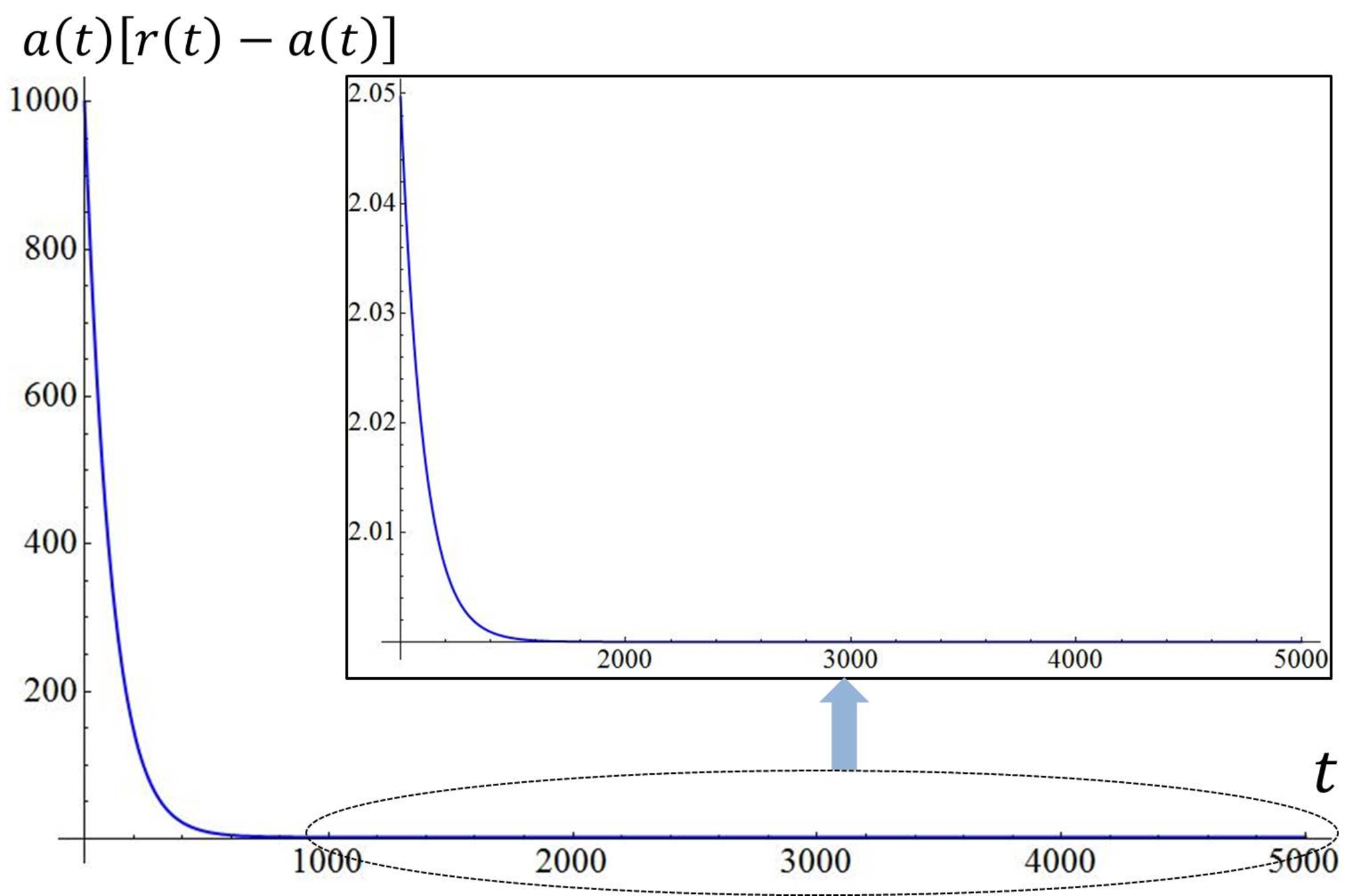
We give a numerical demonstration of 11. We consider a simple case where $\sigma(a)=k=$ const. in 2, the solution of which is given by $a(t)=[a(0)^{3}-6kt]^{1/3}$ . Using this, we solve 9 numerically for $a(0)=100,~r(0)=110$ , and $k=1$ and obtain Fig. 14. This shows that $r(t)$ approaches $a(t)+\frac{2k}{a(t)}$ as in 11.

Appendix C A multishell model

We introduce a simple model [8] as a concrete example for the new picture in Sec. II.3.

C.1 Single-shell model

In order to construct the self-consistent solution of $G_{\mu\nu}=8\pi G\langle T_{\mu\nu}\rangle$ , we start with a spherically symmetric collapsing null shell. The inside region is flat because of the spherical symmetry. We assume that the outside region is described by the outgoing Vaidya metric [9]:

\mathrm{d}s^{2}=\begin{cases}-\mathrm{d}U^{2}-2\mathrm{d}U\mathrm{d}r+r^{2}\mathrm{d}\Omega^{2}~~{\rm for}~~r\leq r_{s}\\ -\frac{r-a(u)}{r}\mathrm{d}u^{2}-2\mathrm{d}u\mathrm{d}r+r^{2}\mathrm{d}\Omega^{2}~~{\rm for}~~r\geq r_{s}\end{cases}

(145)

Here $r_{s}$ is the radius of the shell, $M(u)=\frac{a(u)}{2G}$ is the Bondi mass, and $U$ and $u$ are the outgoing null coordinates in the Eddington-Finkelstein coordinates for the inside and outside, respectively. See Fig. 15.

In Ref.[8], we have shown that the self-consistent solution is obtained by solving

\frac{r_{s}(u)-a(u)}{r_{s}(u)}\mathrm{d}u=-2\mathrm{d}r_{s}=\mathrm{d}U

(146)

and

\frac{\mathrm{d}a}{\mathrm{d}u}=-\frac{l_{p}^{2}}{8\pi}\{u,U\}~,

(147)

provided that the radiation is massless, and only the s-wave is considered in the eikonal approximation. Here, $\{u,U\}$ is the Schwarzian derivative, which is given by $\{u,U\}\equiv\frac{\ddot{U}(u)^{2}}{\dot{U}(u)^{2}}-\frac{2\dddot{U}(u)}{3\dot{U}(u)}$ . Equation 146 indicates that the motion of the shell is lightlike both in the inside and the outside regions. Equation 147 is equivalent to the Einstein equation $G_{\mu\nu}=8\pi G\langle T_{\mu\nu}\rangle$ because the only nonzero components of $G_{\mu\nu}$ and $\langle T_{\mu\nu}\rangle$ are $G_{uu}=-\frac{\dot{a}(u)}{r^{2}}$ and $\langle T_{uu}\rangle=\frac{1}{4\pi r^{2}}\frac{\hbar}{16\pi}\{u,U\}$ .

C.2 Generalization to multishells

It is easy to generalize the above model to the case of multishells. We consider $n$ shells of which the radii are denoted by $r_{i}$ $(i=1,...n)$ . See Fig. 16.

The metric of the region between $r_{i}$ and $r_{i+1}$ is described by

\mathrm{d}s^{2}_{i}=-\frac{r-a_{i}(u_{i})}{r}\mathrm{d}u_{i}^{2}-2\mathrm{d}u_{i}\mathrm{d}r+r^{2}\mathrm{d}\Omega^{2}~,

(148)

where $u_{i}$ is the local time and $\frac{a_{i}(u_{i})}{2G}$ is the mass in the $i$ th shell. The junction condition of each time coordinate $u_{i}$ is given as 146 by

\frac{r_{i}-a_{i}}{r_{i}}\mathrm{d}u_{i}=-2\mathrm{d}r_{i}=\frac{r_{i}-a_{i-1}}{r_{i}}\mathrm{d}u_{i-1}~~{\rm for}~~i=1,...n~,

(149)

where we regard $a_{0}=0$ and $u_{0}=U$ for the flat space. This is equivalent to

\frac{\mathrm{d}r_{i}}{\mathrm{d}u_{i}}=-\frac{r_{i}-a_{i}}{2r_{i}}~,

(150)

and

\frac{\mathrm{d}u_{i}}{\mathrm{d}u_{i-1}}=\frac{r_{i}-a_{i-1}}{r_{i}-a_{i}}=1+\frac{a_{i}-a_{i-1}}{r_{i}-a_{i}}~.

(151)

The Einstein equation 147 holds for each shell,

\frac{\mathrm{d}a_{i}}{\mathrm{d}u_{i}}=-\frac{Nl_{p}^{2}}{8\pi}\{u_{i},U\}~,

(152)

where the degrees of freedom of the fields $N$ have been introduced.

The coupled equations 149 and 152 can be solved by the following ansatz:

\frac{\mathrm{d}a_{i}}{\mathrm{d}u_{i}}=-\frac{C}{a_{i}^{2}},

(153)

r_{i}=a_{i}-2a_{i}\frac{\mathrm{d}a_{i}}{\mathrm{d}u_{i}}=a_{i}+\frac{2C}{a_{i}}~.

(154)

Equation 153 means that each shell behaves like the conventional evaporating black hole, and 154 indicates that each shell has reached the asymptotic radius as in 11.

First, Eq. 154 solves 150 as in 11. Next, we solve 151 with the ansatz. We define $\eta_{i}$ by

\eta_{i}\equiv\log\frac{\mathrm{d}U}{\mathrm{d}u_{i}}~.

(155)

Then, we have

$\displaystyle\eta_{i}-\eta_{i-1}$	$\displaystyle=\log\frac{\frac{\mathrm{d}U}{\mathrm{d}u_{i}}}{\frac{\mathrm{d}U}{\mathrm{d}u_{i-1}}}=-\log\frac{\mathrm{d}u_{i}}{\mathrm{d}u_{i-1}}$
	$\displaystyle=-\log\left(1+\frac{a_{i}-a_{i-1}}{r_{i}-a_{i}}\right)$
	$\displaystyle\approx-\frac{a_{i}-a_{i-1}}{r_{i}-a_{i}}\approx-\frac{a_{i}-a_{i-1}}{\frac{2C}{a_{i}}}$
	$\displaystyle\approx-\frac{1}{4C}\left(a_{i}^{2}-a_{i-1}^{2}\right)~.$	(156)

Here, at the second line, we use 151; at the third line, we assume $\frac{a_{i}-a_{i-1}}{\frac{2C}{a_{i}}}\ll 1$ , which is satisfied for the case of continuous distribution; and at the last line, we approximate $2a_{i}\approx a_{i}+a_{i-1}$ . With the boundary conditions $\eta_{0}=a_{0}=0$ , we obtain

\eta_{i}=-\frac{1}{4C}a_{i}^{2}.

(157)

Finally, we check 152. Because the Schwarzian derivative $\{u_{i},U\}$ is written as

\{u_{i},U\}=\frac{1}{3}\left(\frac{\mathrm{d}\eta_{i}}{\mathrm{d}u_{i}}\right)^{2}-\frac{2}{3}\frac{\mathrm{d}^{2}\eta_{i}}{\mathrm{d}u_{i}^{2}}~,

(158)

we obtain

\{u_{i},U\}\approx\frac{1}{12}\frac{1}{a_{i}^{2}}~.

(159)

Here, we have used 153 and 157 to obtain

\frac{\mathrm{d}\eta_{i}}{\mathrm{d}u_{i}}=-\frac{1}{2C}a_{i}\frac{\mathrm{d}a_{i}}{\mathrm{d}u_{i}}=\frac{1}{2a_{i}}~.

(160)

Therefore, Eq. 152 is satisfied if

C=\frac{Nl_{p}^{2}}{96\pi}.

(161)

In particular, the outermost shell ( $n$ th shell) satisfies

\frac{\mathrm{d}a}{\mathrm{d}u}=-\frac{C}{a^{2}},

(162)

which indicates that the entire system behaves like the conventional evaporating black hole when it is observed from the outside.

Appendix D Hawking radiation in the new picture

We show that the metric of the new picture of black holes indeed creates radiation from the vacuum which obey a Planck-like distribution with the Hawking temperature 17 [49]. We start with the general form of the spherically symmetric metric in the Eddington-Finkelstein-like coordinates:

\mathrm{d}s^{2}=-q(u,r)\left(\frac{h(u,r)}{r}\mathrm{d}u+2\mathrm{d}r\right)\mathrm{d}u+r^{2}\mathrm{d}\Omega^{2}~.

(163)

See Fig. 17.

We assume that the metric near the surface, $R_{F}<r\leq R$ , is given by 74. Rigorously speaking, the values of $f$ and $\sigma$ there for the evaporating black hole may be different from those of the adiabatically formed one. Here we simply assume that they are the same. On the other hand, the deeper region, $0\lesssim r\leq R_{F}$ , need not be the same as 74, but the metric there is frozen in time. We further assume that there remains a small flat spacetime around the origin:

\mathrm{d}s^{2}=-\mathrm{d}U^{2}-2\mathrm{d}U\mathrm{d}r+r^{2}\mathrm{d}\Omega^{2}~.

(164)

We consider the s-wave of a massless real scaler field $\phi(x)$ and solve the Heisenberg equation using the eikonal approximation [1]. In this approximation, the reflection of the radiation is not considered, and $f(r)$ becomes zero. The Hawking radiation is created by the time evolution of the field along a ray that starts from the flat space before the collapse, goes through the center, and passes the collapsing matter (see Fig. 17). We focus here on a time interval around $u_{*}$ , $I(u_{*})=[u_{*}-ka(u_{*}),u_{*}+ka(u_{*})]$ , where $k\sim 1$ . By putting $\phi=r^{-1}e^{i\frac{S(u,r)}{\hbar}}$ , the Klein-Gordon equation $\nabla^{2}\phi=0$ in the metric 163 becomes

\left[\frac{1}{q}\partial_{u}-\frac{h}{2rq}\partial_{r}\right]S~\partial_{r}S=0~,

(165)

in the leading approximation of the $\hbar$ expansion. Here, the ingoing and outgoing radial null vectors are given by $\bm{k}=\frac{1}{q}\partial_{u}-\frac{h}{2rq}\partial_{r}$ and $\bm{l}=\partial_{r}$ , respectively. Therefore, we obtain the outgoing eikonal solution

\phi_{out}=\frac{e^{i\frac{S_{out}(u)}{\hbar}}}{r}~.

(166)

We assume that the field was in the vacuum state before the collapse. Therefore, in the Heisenberg picture, the state should satisfy

a_{\omega}|0\rangle=0~,

(167)

where $a_{\omega}$ is the coefficient of $e^{-i\omega U}$ for $\omega>0$ in the outgoing component of $\phi~$ :

\phi=\int_{0}^{\infty}\frac{\mathrm{d}\omega}{\sqrt{2\pi}}\frac{1}{\sqrt{2\omega}}\left(\frac{e^{-i\omega U}}{\sqrt{4\pi}r}a_{\omega}+\frac{e^{i\omega U}}{\sqrt{4\pi}r}a_{\omega}^{\dagger}\right)~.

(168)

Because of 166, the field which has evolved is given by

\phi=\int_{0}^{\infty}\frac{\mathrm{d}\omega}{\sqrt{2\pi}}\frac{1}{\sqrt{2\omega}}\left(\frac{e^{-i\omega U(u)}}{\sqrt{4\pi}r}a_{\omega}+\frac{e^{i\omega U(u)}}{\sqrt{4\pi}r}a_{\omega}^{\dagger}\right)~.

(169)

On the other hand, this can also be expressed in terms of the modes in the future infinity:

\phi=\int_{0}^{\infty}\frac{\mathrm{d}\omega}{\sqrt{2\pi}}\frac{1}{\sqrt{2\omega}}\left(\frac{e^{-i\omega u}}{\sqrt{4\pi}r}b_{\omega}+\frac{e^{i\omega u}}{\sqrt{4\pi}r}b_{\omega}^{\dagger}\right)~.

(170)

Generally, two operators $a_{\omega}$ and $b_{\omega^{\prime}}$ are related as

b_{\omega}=\int^{\infty}_{-\infty}\mathrm{d}\omega^{\prime}A_{\omega\omega^{\prime}}a_{\omega^{\prime}}=\int^{\infty}_{0}\mathrm{d}\omega^{\prime}(A_{\omega\omega^{\prime}}a_{\omega^{\prime}}+A_{\omega,-\omega^{\prime}}a_{\omega^{\prime}}^{\dagger})~.

(171)

From 169, 170, and 171, we obtain

A_{\omega,-\omega^{\prime};u_{*}}=\frac{1}{2\pi}\sqrt{\frac{\omega}{\omega^{\prime}}}\int_{-\infty}^{\infty}\mathrm{d}ue^{i\omega u}e^{i\omega^{\prime}U(u)}~.

(172)

Here, we have extended the integration region from $I(u_{*})$ to $[-\infty,\infty]$ , which does not affect the following calculation [1, 8, 17] [50]. From 171, we obtain the expectation value of the number of the particles:

\langle 0|b_{\omega}^{\dagger}b_{\omega}|0\rangle_{u_{*}}=\int_{0}^{\infty}\mathrm{d}\omega^{\prime}|A_{\omega,-\omega^{\prime};u_{*}}|^{2}~.

(173)

Then, we estimate $U(u)$ , which is the relation between the outside time $u$ and the time $U$ around the origin. In the metric 163, the ingoing radial geodesic $r(u)$ is given by $\frac{1}{q}\frac{\mathrm{d}r}{\mathrm{d}u}=-\frac{h}{2rq}$ , and $q(u,r(u))\mathrm{d}u$ corresponds to the local time at $r=r(u)$ . Because $u$ is the outside time and $q(u,r=R)=1$ , we have

	$\displaystyle\frac{\mathrm{d}U(u)}{\mathrm{d}u}$	$\displaystyle=q(u,r\sim 0)=\frac{q(u,r\sim 0)}{q(u,r=R_{F})}q(u,r=R_{F})$
		$\displaystyle=Ce^{-\int^{R(u)}_{R_{F}}\mathrm{d}r\frac{r}{2\sigma(r)}}\approx Ce^{-\frac{R(u)^{2}-R_{F}^{2}}{4\sigma(R(u))}}~.$		(174)

Here, in the interval $I(u_{*})$ , the deeper region between $0\lesssim r\leq R_{F}$ is frozen in time so that $\frac{q(u,r\sim 0)}{q(u,r=R_{F})}$ is a constant, $C$ . On the other hand, the region near the surface, $R_{F}<r\leq R(u)$ , is described by the interior metric of 74 with $f=0$ . Next, we expand $R(u)$ around $u_{*}$ as

	$\displaystyle R(u)$	$\displaystyle\approx R(u_{})+\frac{\mathrm{d}R}{\mathrm{d}u}(u_{})(u-u_{*})$
		$\displaystyle=R(u_{})-\frac{\sigma(R(u_{}))}{R(u_{})^{2}}(u-u_{})~,$		(175)

where we have used the geodesic equation in 74, $\frac{\mathrm{d}R}{\mathrm{d}u}=-\frac{\sigma(R)}{R^{2}}$ . Putting $R(u)^{2}\approx R(u_{*})^{2}-\frac{2\sigma(R(u_{*}))}{R(u_{*})}(u-u_{*})$ into 174, we have $\frac{\mathrm{d}U(u)}{\mathrm{d}u}\approx C^{\prime}e^{\frac{u}{2R(u_{*})}}$ . Thus, we obtain

U(u;u_{*})=D+2R(u_{*})C^{\prime}e^{\frac{u}{2R(u_{*})}}~,

(176)

where $D$ and $C^{\prime}$ are constants.

Now, we can evaluate 172. Using 176 and continuing analytically [1], we have

A_{\omega,-\omega^{\prime};u_{*}}=\frac{1}{2\pi}\sqrt{\frac{\omega}{\omega^{\prime}}}2R(u_{*})e^{-\pi\omega R(u_{*})}\Gamma(2i\omega R(u_{*}))~,

(177)

where an irrelevant overall phase factor has been dropped. Then, employing the formula $|\Gamma(ix)|^{2}=\frac{\pi}{x\sinh(\pi x)}$ for $x\in\mathbb{R}$ and considering wave packets in 173 [1, 17], we obtain

\langle 0|b_{\omega}^{\dagger}b_{\omega}|0\rangle_{u_{*}}=\frac{1}{e^{\frac{\hbar\omega}{T_{H}(u_{*})}}-1}~,

(178)

where

T_{H}(u)=\frac{\hbar}{4\pi R(u)}\approx\frac{\hbar}{4\pi a(u)}~.

(179)

This agrees with the Hawking temperature [1] but changes in time slowly according to 2. The above analysis has shown that the Hawking radiation is created in any collapsing process as long as the region near the surface becomes the asymptotic spacetime described by 74. In particular, the existence of the horizon is not necessary.

Appendix E Examples of the interior structure

Simple examples would be helpful to understand the new picture. We consider two macroscopic shells with radii $r_{1}$ and $r_{2}$ , where $r_{1}<r_{2}$ . We assume initially they have the same energy $M$ . Then, the Schwarzschild radius of the total system and the inner shell are $a_{2}=4GM$ and $a_{1}=2GM$ , respectively. Although in the real system the energy distributes continuously, for simplicity we consider two thin shells. See Fig. 18.

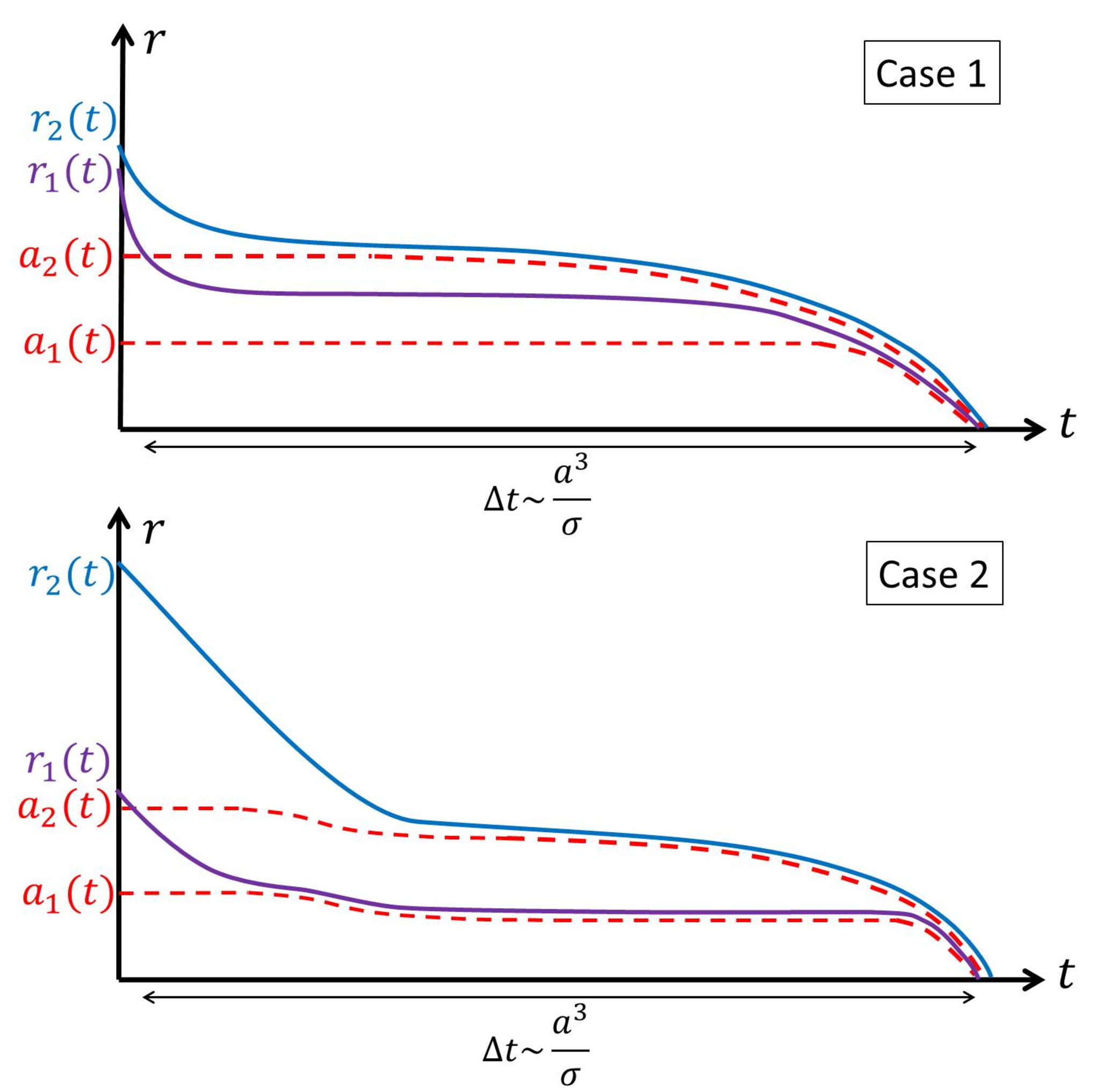
We consider the following two cases. In one case the initial values of the radii are very close, for example, $r_{1}=3a_{1}$ and $r_{2}=3a_{1}+\Delta r$ , where $\Delta r\ll a_{1}$ (see the upper panel of Fig. 18). Then, shell 2 reaches $r=R(a_{2})$ earlier than shell 1 reaches $r=R(a_{1})$ because the two shells have started from almost the same positions but $R(a_{2})$ is significantly larger than $R(a_{1})$ . When shell 2 reaches $r=R(a_{2})$ , time inside shell 2 is frozen, and $r_{1}$ stays almost constant. At the same time, shell 2 starts emitting the Hawking radiation. Thus, only shell 2 evaporates until its energy is exhausted. After that, shell 1 begins to approach to $R(a_{1})$ and eventually evaporates.

In the other case, shell 1 reaches $r=R(a_{1})$ earlier than shell 2 reaches $r=R(a_{2})$ . Such a case occurs if the initial value of $r_{1}$ is close to $R(a_{1})$ but $r_{2}$ is not so close to $R(a_{2})$ (see the lower panel of Fig. 18). Then, shell 1 reaches $R(a_{1})$ before it is frozen by shell 2, and some part of it evaporates until shell 2 reaches $R(a_{2})$ . Then, shell 1 stops radiating, and only shell 2 emits the energy. After this, the same thing occurs as in the first case.

Appendix F Surface energy density and pressure on the evaporating shell

We derive 45 and 46 from the Barrabes-Israel junction condition [25] following the formalism in Ref.[26]. We consider an evaporating shell with initial energy $\epsilon(0)\sim\frac{\hbar}{a}$ which approaches the evaporating core with $a^{\prime}(t^{\prime})$ as in Fig. 2. The metric is given by 20, and we denote the position of the shell by $r_{s}$ . We take the ingoing and outgoing null vectors as $\bm{k}=f^{-1}\partial_{T}-\partial_{r}$ and $\bm{l}=\frac{1}{2}\partial_{T}+\frac{f}{2}\partial_{r}$ , respectively, so that $\bm{k}\cdot\bm{l}=-1$ . Here, $T=t$ and $f=1-\frac{a}{r}$ for $r>r_{s}$ , while $T=t^{\prime}$ and $f=1-\frac{a^{\prime}}{r}$ for $r<r_{s}$ . Note that the null vector $\bm{k}$ satisfies the geodesic equation $\nabla_{\bm{k}}k^{\mu}=\kappa k^{\mu}$ with

\kappa=-f^{-2}\partial_{T}f~.

(180)

We assume that the shell moves along $\bm{k}$ and denote its locus by ${\cal N}$ . The transverse curvature of the null hypersurface ${\cal N}$ is given by

C_{ab}=\frac{1}{2}(\pounds_{\bm{l}}g_{\mu\nu})e^{\mu}_{a}e^{\nu}_{b}.

(181)

Here $\pounds_{\bm{l}}$ is the Lie derivative along $\bm{l}$ , and $\{\bm{e}_{a}\}=\{\bm{e}_{\lambda}=\bm{k},\bm{e}_{\theta}=\partial_{\theta},\bm{e}_{\varphi}=\partial_{\varphi}\}$ is the basis on ${\cal N}$ . Using another expression $C_{ab}=-l_{\nu}e^{\mu}_{a}\nabla_{\mu}e^{\nu}_{b}$ (see Ref. [26]), we obtain

C_{\lambda\lambda}=\kappa,~C_{AB}=\frac{f}{2r}\sigma_{AB}~,

(182)

where $\sigma_{AB}$ is the 2-metric on the shell such that $\sigma_{AB}\mathrm{d}\theta^{A}\mathrm{d}\theta^{B}=r^{2}\mathrm{d}\theta^{2}+r^{2}\sin^{2}\theta\mathrm{d}\varphi^{2}$ with $\theta^{A}=\{\theta,\varphi\}$ . Thus, we obtain the formula 45 for the surface energy density $\epsilon_{2d}$ and pressure $p_{2d}$ :

$\displaystyle\epsilon_{2d}$	$\displaystyle=-\frac{1}{8\pi G}\sigma^{AB}[C_{AB}]=\frac{\epsilon}{4\pi r_{s}^{2}}~,$
$\displaystyle p_{2d}$	$\displaystyle=-\frac{1}{8\pi G}[C_{\lambda\lambda}]=-\frac{1}{8\pi G}[\kappa]$
	$\displaystyle=-\frac{r_{s}}{8\pi G(r_{s}-a)^{2}}\left(\frac{\mathrm{d}a}{\mathrm{d}t}-\left(\frac{r_{s}-a}{r_{s}-a^{\prime}}\right)^{2}\frac{\mathrm{d}a^{\prime}}{\mathrm{d}t^{\prime}}\right)~.$	(183)

Here, $[A]\equiv A|_{r\to r_{s}+0}-A|_{r\to r_{s}-0}$ for a quantity $A$ , and $\epsilon=\frac{a-a^{\prime}}{2G}$ is the energy of the shell.

Next, we show 46. Suppose that the shell has come close to the core as in stage II of Fig. 2, where $r_{s}=a+\frac{2\sigma(a)}{a}$ . Using 14, 23, $\Delta a\sim\frac{l_{p}^{2}}{a}$ , and $\frac{1}{a^{\prime 2}}\approx\frac{1}{a^{2}}\left(1+\frac{2\Delta a}{a}\right)$ , $p_{2d}$ in 183 becomes

	$\displaystyle p_{2d}$
$\displaystyle\approx$	$\displaystyle\frac{a}{8\pi G}\frac{a^{2}}{(2\sigma)^{2}}\left(\frac{2\sigma(a)}{a^{2}}-\left(1-2\frac{a\Delta a}{2\sigma(a)}\right)\frac{2\sigma(a)}{a^{2}}\left(1+\frac{2\Delta a}{a}\right)\right)$
$\displaystyle\approx$	$\displaystyle\frac{a^{2}\Delta a}{16\pi G\sigma^{2}}$
$\displaystyle\sim$	$\displaystyle\frac{a}{GN^{2}l_{p}^{2}}~.$	(184)

Appendix G Exponential decrease in the energy of the collapsing matter

Here we derive 93. We consider ingoing matter with radius $r=r(t)$ and width $\Delta r(t)$ , in the outermost region of the evaporating black hole with radius $a(t)$ . Here we assume the metric is given by 72 and examine the time evolution of the ADM energy of the shell $\epsilon(t)$ , which is expressed as

\epsilon(t)=4\pi r(t)^{2}\rho(r(t))\Delta r(t)=\frac{1}{2G}\Delta r(t)~,

(185)

where $\rho=-\langle T^{t}{}_{t}\rangle=\frac{1}{8\pi Gr^{2}}$ because of 78.

We first consider the motion of a test particle in 72. If it is ultrarelativistic, it satisfies

\frac{\mathrm{d}r}{\mathrm{d}t}=-\frac{1}{B}e^{\frac{A}{2}}~.

(186)

Taking the difference of this equation with respect to $r$ , we obtain

\frac{\mathrm{d}\Delta r}{\mathrm{d}t}=\left(\frac{\partial_{r}B}{B}-\frac{1}{2}\partial_{r}A\right)\frac{e^{\frac{A}{2}}}{B}\Delta r\approx-\frac{r}{2\sigma(1+f)}\frac{e^{\frac{A}{2}}}{B}\Delta r~,

(187)

where we have used 71 and 65. This can be rewritten in terms of the local time $\mathrm{d}\tau=\frac{1}{\sqrt{B(r)}}e^{\frac{A(r)}{2}}\mathrm{d}t$ , as

\frac{\mathrm{d}\Delta r}{\mathrm{d}\tau}=-\frac{1}{\sqrt{2\sigma}(1+f)}\Delta r~,

(188)

and the solution is given by

\Delta r(\tau)=\Delta r(0)e^{-\frac{\tau}{\sqrt{2\sigma}(1+f)}}~.

(189)

Therefore, the time evolution of the local energy $\epsilon_{local}=\frac{\epsilon}{\sqrt{-g_{tt}}}$ is given by

\epsilon_{local}(\tau)=\epsilon_{local}(0)e^{-\frac{\tau}{\sqrt{2\sigma}(1+f)}}~.

(190)

Appendix H Entropy of the stationary black hole

We consider the stationary black hole that is formed adiabatically in the heat bath and evaluate the total entropy by summing up the contribution from each piece in the interior. Here, we approximate the interior as one-dimensional massless radiation with local equilibrium. Because the local energy of particles is ultrarelativistic, and the ingoing and outgoing energy flux are balanced at each $r$ , it is reasonable to consider such a model.

Then, the Gibbs relation for one-dimensional radiation [5] should be satisfied,

u+p=T_{local}s,~~~u=p~,

(191)

where $u,~p,~T_{local}$ , and $s$ are one-dimensional internal energy density, pressure, local temperature, and entropy density, respectively. In the following, we evaluate

s=2\frac{u}{T_{local}}

(192)

and integrate it over the inside of the black hole by using the metric 72.

We first evaluate $u$ . The general mass formula 39 indicates that $\rho=-\langle T^{t}{}_{t}\rangle$ can be regarded as the four-dimensional energy density in the local inertial frame. This is because the integration measure is the same as the ordinary flat space, and the diagonal component $T^{t}{}_{t}$ is the same as $T^{\tau}{}_{\tau}$ for the stationary state. Then, the one-dimensional energy density, that is, the proper energy per proper length, is given by [51]

e=4\pi r^{2}\rho~.

(193)

Here, by noting that the ingoing and outgoing energy flows are balanced in the stationary state, the energy flow only in one direction should be considered to count the entropy in 192. Therefore, by using 78, we can evaluate the one-dimensional internal energy density as

u=\frac{1}{2}e=\frac{1}{4G}.

(194)

Now we can evaluate the entropy. From 192, 194, and 101, we obtain

s(r)=2\pi\frac{\sqrt{2\sigma(r)}}{l_{p}^{2}}~,

(195)

which indicates that $\sqrt{\sigma}/l_{p}^{2}$ bits are stored per unit proper length, as discussed in Ref. [24]. Integrating this from $r\sim 0$ to $r=R(a)=a+\frac{2\sigma(a)}{a}$ , we have

$\displaystyle S_{BH}$	$\displaystyle=\int_{0}^{R(a)}\mathrm{d}r\sqrt{g_{rr}(r)}s(r)$
	$\displaystyle=\int_{0}^{R(a)}\mathrm{d}r\frac{r}{\sqrt{2\sigma(r)}}2\pi\frac{\sqrt{2\sigma(r)}}{l_{p}^{2}}$
	$\displaystyle\approx\frac{\pi a^{2}}{l_{p}^{2}}=\frac{A}{4l_{p}^{2}}~,$	(196)

which agrees with the Bekenstein-Hawking formula. Thus, we have seen that the black hole entropy is stored in the interior structure.

Appendix I Surface of the rotating black hole

In Sec. VI.1 we analyze the motion of a test particle in the evaporating Kerr metric, and show that the notion of surface is valid even for the rotating black holes. In this Appendix, we derive the three equations 121, 122 and 123, which play a crucial role for the existence of the surface.

If the black hole is not very close to extremal, the relevant time scales are similar to those of the spherically symmetric black holes. The time scale of the change of the mass $M(t)$ and the angular momentum $j(t)$ is about $M^{3}$ , while the test particle approaches the horizon in the time scale of $\sim M$ . Therefore it is enough to analyze the equation of motion of the test particle for constant $M$ and $j$ , and then replace them to the time-dependent ones.

In order to do that, we consider the Hamilton-Jacobi equation for a massive particle with mass $m$ [26] in the Kerr metric 118:

0=g^{\mu\nu}\partial_{\mu}S\partial_{\nu}S+m^{2}.

(197)

As usual, because of the cylindrical symmetry, we can set

S(t,r,\theta,\phi)=-Et+L\phi+W(r,\theta)~.

(198)

By using the inverse metric

		$\displaystyle g^{tt}=-\frac{P}{\Sigma\Delta},~g^{rr}=\frac{\Delta}{\Sigma},~g^{\theta\theta}=\frac{1}{\Sigma},$
		$\displaystyle g^{\phi\phi}=\frac{\Delta-j^{2}\sin^{2}\theta}{\Sigma\Delta\sin^{2}\theta},~g^{t\phi}=-\frac{2Mjr}{\Sigma\Delta}~,$

Eq. 197 becomes

	$\displaystyle 0$	$\displaystyle=-\frac{P}{\Sigma\Delta}E^{2}+\frac{\Delta}{\Sigma}(\partial_{r}W)^{2}+\frac{1}{\Sigma}(\partial_{\theta}W)^{2}$
		$\displaystyle+\frac{\Delta-j^{2}\sin^{2}\theta}{\Sigma\Delta\sin^{2}\theta}L^{2}+2\frac{2Mjr}{\Sigma\Delta}EL+m^{2}~.$		(199)

Multiplying this by $\Sigma$ , we obtain

	$\displaystyle 0$	$\displaystyle=\left(-\frac{1}{\Delta}[(r^{2}+j^{2})^{2}E^{2}+j^{2}L^{2}-4MjrLE]+\Delta(\partial_{r}W)^{2}+(r^{2}+j^{2})m^{2}\right)$
		$\displaystyle~~~~~~~~~~~~~+\left(j^{2}\sin^{2}\theta E^{2}+\frac{L^{2}}{\sin^{2}\theta}+(\partial_{\theta}W)^{2}-j^{2}\sin^{2}\theta m^{2}\right)~.$		(200)

The first and second terms depend only on $r$ and $\theta$ , respectively. Therefore, we can put the first term as a constant, $-C$ , where $C$ is the Carter constant [26], and decompose $W(r,\theta)$ as

W(r,\theta)=w(r)+\Theta(\theta)~.

(201)

Then we have the two ordinary differential equations and obtain the solutions

w(r;E,L,C)=\pm\int^{r}\mathrm{d}r\frac{1}{\Delta}\sqrt{(r^{2}+j^{2})^{2}E^{2}+j^{2}L^{2}-4MjrLE-\Delta[C+(r^{2}+j^{2})m^{2}]}~,

(202)

\Theta(\theta;E,L,C)=\pm\int^{\theta}\mathrm{d}\theta\sqrt{C-\frac{L^{2}}{\sin^{2}\theta}-j^{2}\sin^{2}\theta(E^{2}-m^{2})}~.

(203)

Taking two derivatives of

S=-Et+L\phi+w(r;E,L,C)+\Theta(\theta;E,L,C)

(204)

with respect to $E$ and to $t$ , we have

	$\displaystyle 0$	$\displaystyle=-1\pm\frac{(r_{+}^{2}+j^{2})}{\Delta(r(t))}\frac{\mathrm{d}r(t)}{\mathrm{d}t}$
		$\displaystyle\pm\frac{-Ej^{2}\sin^{2}\theta(t)}{\sqrt{C-\frac{L^{2}}{\sin^{2}\theta(t)}-j^{2}\sin^{2}\theta(t)(E^{2}-m^{2})}}\frac{\mathrm{d}\theta(t)}{\mathrm{d}t}~.$		(205)

We now focus on the region $r\sim r_{+}$ , where $\Delta\sim 0$ . Using $\Delta=(r(t)-r_{+})(r(t)-r_{-})\approx(r(t)-r_{+})(r_{+}-r_{-})$ and $\kappa_{K}=\frac{r_{+}-r_{-}}{2(r_{+}^{2}+j^{2})}$ , from 205 we obtain

		$\displaystyle\frac{\mathrm{d}r(t)}{\mathrm{d}t}=-2\kappa_{K}(r(t)-r_{+})$
		$\displaystyle~~~~\times\left[1\pm\frac{Ej^{2}\sin^{2}\theta(t)}{\sqrt{C-\frac{L^{2}}{\sin^{2}\theta(t)}-j^{2}\sin^{2}\theta(t)(E^{2}-m^{2})}}\frac{\mathrm{d}\theta(t)}{\mathrm{d}t}\right],$		(206)

where we have chosen the sign for the radial ingoing direction. Similarly, taking two derivative of 204 with respect to $C$ and $t$ , we obtain

\frac{\mathrm{d}\theta(t)}{\mathrm{d}t}=\frac{\sqrt{C-\frac{L^{2}}{\sin^{2}\theta(t)}-j^{2}\sin^{2}\theta(t)(E^{2}-m^{2})}}{(r_{+}^{2}+j^{2})E-jL}\frac{\mathrm{d}r(t)}{\mathrm{d}t}~.

(207)

Then substituting this into 206, we have

\frac{\mathrm{d}r(t)}{\mathrm{d}t}=-2\kappa_{K}(r(t)-r_{+})\left[1\pm\frac{Ej^{2}\sin^{2}\theta(t)}{(r_{+}^{2}+j^{2})E-jL}\frac{\mathrm{d}r(t)}{\mathrm{d}t}\right]~.

(208)

The second term in the large bracket in 208 turns out to be of order ${\cal O}(r_{+}^{-2})$ , and it can be neglected compared with the first term. We can show this as follows, Since we consider adiabatic processes, the ingoing energy $E$ should be of the same order as the Hawking temperature, $E\sim T_{H}\sim\frac{1}{r_{+}}$ . The typical angular momentum of the ingoing particles can be estimated as $L\sim$ (impact parameter) $\times$ (energy) $\sim r_{+}E\sim 1$ . Furthermore, as in the spherically symmetric case, we have

r(t)-r_{+}(t)\sim\frac{1}{r_{+}(t)}~,

(209)

which will be shown self-consistently. Using these estimates, we can show the above statement.

Thus, we obtain

\frac{\mathrm{d}r(t)}{\mathrm{d}t}=-2\kappa_{K}(r(t)-r_{+})+{\cal O}(r_{+}^{-3})~,

(210)

which is 121. From this, Eq. 207 can be estimated as

\frac{\mathrm{d}\theta(t)}{\mathrm{d}t}\sim\frac{1}{r_{+}}2\kappa_{K}(r(t)-r_{+})\sim\frac{1}{r_{+}^{3}}~,

(211)

which gives 122.

Finally we examine $\frac{\mathrm{d}\phi(t)}{\mathrm{d}t}$ . Taking two derivatives of 204 with respect to $L$ and $t$ , we have

	$\displaystyle 0$	$\displaystyle=\frac{\mathrm{d}\phi(t)}{\mathrm{d}t}\pm\frac{-a}{\Delta}\frac{\mathrm{d}r(t)}{\mathrm{d}t}$
		$\displaystyle~~~\pm\frac{-\frac{L}{\sin^{2}\theta(t)}}{\sqrt{C-\frac{L^{2}}{\sin^{2}\theta(t)}-j^{2}\sin^{2}\theta(t)(E^{2}-m^{2})}}\frac{\mathrm{d}\theta(t)}{\mathrm{d}t}$
		$\displaystyle=\frac{\mathrm{d}\phi(t)}{\mathrm{d}t}\pm\frac{-a}{\Delta}\frac{\pm\Delta}{r_{+}^{2}+j^{2}}+{\cal O}(r_{+}^{-3})~.$

Thus, we have 123:

\frac{\mathrm{d}\phi(t)}{\mathrm{d}t}=\omega_{H}+{\cal O}(r_{+}^{-3})~.

(212)

References

[1] S. W. Hawking, Commun. Math. Phys. 43, 199 (1975) [Erratum-ibid. 46, 206 (1976)].
[2] G. W. Gibbons and S. W. Hawking, Phys. Rev. D 15, 2752 (1977).
[3] S. W. Hawking, Phys. Rev. D 14, 2460 (1976).
[4] J. D. Bekenstein, Phys. Rev. D 7, 2333 (1973); Phys. Rev. D 9, 3292 (1974).
[5] L. D. Landau and E. M. Lifshitz, Statistical Physics (Butterworth-Heinemann, Oxford, 1984).
[6] We will examine the definition of $\sigma(a)$ more precisely in Sec. II.4.
[7] It gives the energy flow 2 correctly, $-G^{r}{}_{t}=\frac{1}{r^{2}}\frac{\mathrm{d}a}{\mathrm{d}t}$ , but gives the zero energy density, $G^{t}{}_{t}=0$ , although the radiation around the black hole should have the energy density of order $-\langle T^{t}{}_{t}\rangle\sim\frac{N}{\hbar^{3}}T_{H}^{4}\sim\frac{N\hbar}{a^{4}}$ . ( $N$ is the number of species of fields.) However, the effect of the latter is so small that the motion of the test particle is not altered. We can show [8] that the result is not changed even if we take the outgoing Vaidya metric [9] instead of 8 (see also Appendix C). In the case of the stationary black holes in the heat bath, we can regard 8 with $a=$ const. as the approximate solution.
[8] H. Kawai, Y. Matsuo, and Y. Yokokura, Int. J. Mod. Phys. A 28, 1350050 (2013) [arXiv:1302.4733 [hep-th]].
[9] P. C. Vaidya, Proc. Indian Acad. Sci. A 33, 264 (1951).
[10] L. D. Landau and E. M. Lifshitz, The Classical Theory of Fields (Butterworth-Heinemann, Oxford, 1980).
[11] See Appendix I for the precise argument. There we also find that $\frac{\mathrm{d}\theta(t)}{\mathrm{d}t}\sim\frac{\mathrm{d}\phi(t)}{\mathrm{d}t}=\mathcal{O}\left(\frac{l_{p}^{2}}{a^{3}}\right)$ , which indicates that near $r\sim a$ particles move only in the radial direction.
[12] See Appendix A for the case of massive particles.
[13] This notion of boundary is different from the stretched horizon in the membrane paradigm [14] in that we consider the inside of the boundary as well as the outside.
[14] K. S. Thorne, R. H. Price, and D. A. Macdonald (ed.), Black Holes: The Membrane Paradigm, (Yale University, New Haven, CT, 1986); L. Susskind, L. Thorlacius, and J. Uglum, Phys. Rev. D 48, 3743 (1993) [hep-th/9306069].
[15] H. Kawai and Y. Yokokura, Int. J. Mod. Phys. A 30, 1550091 (2015) [arXiv:1409.5784 [hep-th]].
[16] P. M. Ho, JHEP 1508, 096 (2015) [arXiv:1505.02468 [hep-th]].
[17] C. Barcelo, S. Liberati, S. Sonego, and M. Visser, Phys. Rev. D 83, 041501 (2011) [arXiv:1011.5593 [gr-qc]]; JHEP 1102, 003 (2011) [arXiv:1011.5911 [gr-qc]].
[18] In Sec. IV.4 we will check that this result is consistent with the four-dimensional Weyl anomaly.
[19] In Appendix E, we give simple examples of the time evolution of collapsing matter.
[20] Several authors have obtained Penrose diagrams similar to Fig. 4 [21]. However, they have considered the black hole as a compact vacuum region surrounded by a trapped surface, which is different from our approach. There are similar works in which the collapsing objects are described from the point of view of an outside observer before a horizon is formed [22].
[21] V. P. Frolov and G. A. Vilkovisky, Phys. Lett. B 106, 307 (1981); C. R. Stephens, G. ’t Hooft and B. F. Whiting, Class. Quant. Grav. 11, 621 (1994) [gr-qc/9310006]; A. Ashtekar and M. Bojowald, Class. Quant. Grav. 22, 3349 (2005) [gr-qc/0504029]; S. A. Hayward, Phys. Rev. Lett. 96, 031103 (2006) [gr-qc/0506126]; A. Ashtekar, V. Taveras and M. Varadarajan, Phys. Rev. Lett. 100, 211302 (2008) [arXiv:0801.1811 [gr-qc]]; S. Hossenfelder, L. Modesto and I. Premont-Schwarz, Phys. Rev. D 81, 044036 (2010) [arXiv:0912.1823 [gr-qc]]; V. P. Frolov, JHEP 1405, 049 (2014) [arXiv:1402.5446 [hep-th]]; Y. Liu, D. Malafarina, L. Modesto and C. Bambi, Phys. Rev. D 90, 044040 (2014) [arXiv:1405.7249 [gr-qc]]; J. M. Bardeen, arXiv:1406.4098 [gr-qc]; C. Barcelo, R. Carballo-Rubio, L. J. Garay and G. Jannes, arXiv:1409.1501 [gr-qc].
[22] G. L. Alberghi, R. Casadio, G. P. Vacca and G. Venturi, Phys. Rev. D 64, 104012 (2001) [gr-qc/0102014]; T. Vachaspati, D. Stojkovic and L. M. Krauss, Phys. Rev. D 76, 024005 (2007) [gr-qc/0609024]; A. Saini and D. Stojkovic, Phys. Rev. Lett. 114, no. 11, 111301 (2015) [arXiv:1503.01487 [gr-qc]].
[23] The detailed mechanism will be discussed in the next section.
[24] From this, we can conclude that the entropy per unit proper length is given by $s\sim\frac{\sigma/l_{p}^{2}}{\Delta l}\sim\frac{\sqrt{\sigma}}{l_{p}^{2}}$ . In Appendix H, we check that this is integrated to reproduce the entropy area law.
[25] C. Barrabes and W. Israel, Phys. Rev. D 43, 1129 (1991).
[26] E. Poisson, A Relativistic Toolkit (Cambridge, 2004).
[27] See also J. Abedi and H. Arfaei, arXiv:1506.05844 [gr-qc].
[28] S. L. Braunstein, S. Pirandola and K. Zyczkowski, Phys. Rev. Lett. 110, no. 10, 101301 (2013) [arXiv:0907.1190 [quant-ph]]; A. Almheiri, D. Marolf, J. Polchinski and J. Sully, JHEP 1302, 062 (2013) [arXiv:1207.3123 [hep-th]];
[29] C. G. Callan, Jr., S. B. Giddings, J. A. Harvey and A. Strominger, Phys. Rev. D 45, 1005 (1992) [hep-th/9111056]; J. G. Russo, L. Susskind and L. Thorlacius, Phys. Rev. D 46, 3444 (1992) [hep-th/9206070]; J. G. Russo, L. Susskind and L. Thorlacius, Phys. Rev. D 47, 533 (1993) [hep-th/9209012].
[30] D. N. Page, Phys. Rev. Lett. 71, 1291 (1993) [gr-qc/9305007]; Phys. Rev. Lett. 71, 3743 (1993) [hep-th/9306083].
[31] J. Polchinski, String Theory vol II (Cambridge Univ. Press, Cambridge, 1998).
[32] In Ref [8], based on this idea, a many-shell model is used to construct the self-consistent interior metric, which is essentially the same as 72.
[33] In this sense, the ordinary evaporation of the black hole in the vacuum is not completely adiabatic because $a$ changes by $\Delta a\sim\frac{\sigma}{a}$ in the time scale $a$ [as 25], which is shorter than $a\log\frac{a}{l_{p}}$ . We can also estimate the entropy production (see Appendix A).
[34] This can also be understood as follows. If we focused on $r\sim 0$ , the leading behavior would be given by $R\sim\frac{1}{r^{2}},~~~\sqrt{R_{\mu\nu}R^{\mu\nu}},~\sqrt{R_{\mu\nu\alpha\beta}R^{\mu\nu\alpha\beta}}\sim\frac{\sigma}{r^{4}}$ , which would diverge at $r=0$ , but the macroscopically large quantity $a$ does not appear in the coefficients. More concretely, we estimate the size of the world line along $r={\rm const.}\sim l_{p}$ for the evaporating black hole with $a(t)$ : $\int\sqrt{-\mathrm{d}s^{2}}\sim\int\mathrm{d}te^{-\int^{a(t)}_{l_{p}}\mathrm{d}r^{\prime}\frac{r^{\prime}}{2(1+f(r^{\prime}))\sigma(r^{\prime})}}\sim\int e^{-\frac{a(t)^{2}}{4(1+f)\sigma}}\mathrm{d}t=\int\mathrm{d}a\frac{\mathrm{d}t}{\mathrm{d}a}e^{-\frac{a^{2}}{4(1+f)\sigma}}\sim\frac{1}{\sigma}\int_{0}^{\infty}\mathrm{d}aa^{2}e^{-\frac{a^{2}}{4(1+f)\sigma}}\sim\sqrt{\sigma}$ . From this and 75, we find that the curvature radius and lifetime of the would-be timelike singularity around the origin is small and controllable in the sense that it can be removed by introducing a string of the size $\sim\sqrt{\sigma}$ surrounding the origin. This contrasts to the macroscopically large spacelike singularity of the vacuum Schwarzschild black hole solution, $\sqrt{R_{\mu\nu\alpha\beta}R^{\mu\nu\alpha\beta}}\sim\frac{a}{r^{3}}$ .
[35] Note here that the energy-momentum tensor jumps at $r=R(a)$ while the Israel junction condition is satisfied [26, 36]. Such a rapid change would become smooth if we consider the time evolution of the outermost region more precisely.
[36] W. Israel, Nuovo Cimento 44B, 1 (1966).
[37] This is singular at $r=0$ . However, as we have discussed in 76, this solution is valid only in the region $\sqrt{\sigma}\lesssim r\leq R(a)$ , where $-\langle T^{t}{}_{t}\rangle\lesssim\frac{1}{G\sigma}$ is not trans-Planckian.
[38] M. J. Duff, Nucl. Phys. B 125, 334 (1977).
[39] N. D. Birrell and P. C. W. Davies, Quantum Fields in Curved space (Cambridge Univ. Press, Cambridge, 1982).
[40] We assume that the coefficients of the higher-curvature terms in the action are renormalized to order 1. However, $\alpha$ and $\gamma$ are proportional to the degrees of freedom $N$ because they are not canceled by counterterms.
[41] We can also check that the exterior metrics in 72 and 74 are well-approximated solutions of the self-consistent equation including the Weyl anomaly because we have $8\pi G\langle T^{\mu}{}_{\mu}\rangle\sim\frac{l_{p}^{2}a^{2}}{r^{4}}\approx 0$ and $G^{\mu}{}_{\mu}=0$ for $r>a$ .
[42] S. M. Christensen and S. A. Fulling, Phys. Rev. D 15, 2088 (1977); E. Mottola and R. Vaulin, Phys. Rev. D 74, 064004 (2006) [gr-qc/0604051].
[43] S. P. Robinson and F. Wilczek, Phys. Rev. Lett. 95, 011303 (2005) [gr-qc/0502074]; S. Iso, H. Umetsu and F. Wilczek, Phys. Rev. Lett. 96, 151302 (2006) [hep-th/0602146]; Phys. Rev. D 74, 044017 (2006) [hep-th/0606018].
[44] This is consistent with a discussion based on the spectral representation [45].
[45] D. M. Capper and M. J. Duff, Nucl. Phys. B 82, 147 (1974); A. Cappelli, D. Friedan and J. I. Latorre, Nucl. Phys. B 352, 616 (1991).
[46] P. C. W. Davies, S. A. Fulling and W. G. Unruh, Phys. Rev. D 13, 2720 (1976); Y. Habara, H. B. Nielsen and M. Ninomiya, arXiv:1503.05340 [hep-th].
[47] It is given by $\frac{\mathrm{d}S}{\mathrm{d}t}\propto-AT^{3}$ [5]. Using $A=4\pi r_{+}^{2}$ , $T=\frac{\kappa_{RN}}{2\pi}$ , and $S=\pi r_{+}^{2}$ , we have 107.
[48] V. De La Cruz and W. Israel, Phys. Rev. 170, 1187 (1968).
[49] A similar derivation is done in Ref. [8]. However, we consider here the general interior metric.
[50] Equation 172 is the same as that of the Klein-Gordon inner product [39] if we use such a Cauchy surface that includes as a part the surface $R(u)$ for $I(u_{*})$ .
[51] We can check this directly from the Hamiltonian $H=\int dr4\pi r^{2}\sqrt{-g_{tt}g_{rr}}\frac{1}{2}[-g^{tt}(\partial_{t}\phi)^{2}+g^{ii}(\partial_{i}\phi)^{2}]\equiv\int dr{\cal H}_{r}$ , where ${\cal H}_{r}$ is the Hamiltonian density per unit radial coordinate. Using $\rho\equiv-T^{t}{}_{t}=\frac{1}{2}[-g^{tt}(\partial_{t}\phi)^{2}+g^{ii}(\partial_{i}\phi)^{2}]$ , we have ${\cal H}_{r}=4\pi r^{2}\sqrt{-g_{tt}g_{rr}}\rho$ . Therefore, the one-dimensional energy density $e$ is given by $e=\frac{dE_{local}}{dl_{local}}=\frac{{\cal H}_{r}}{\sqrt{-g_{tt}g_{rr}}}=4\pi r^{2}\rho$ , because $dE_{local}=\frac{{\cal H}_{r}}{\sqrt{-g_{tt}}}dr$ , and $dl_{local}=\sqrt{g_{rr}}dr$ .

Interior of Black Holes and Information Recovery

Abstract

pacs

I Introduction

II New picture of black holes

II.1 Conventional picture of black holes

II.2 Motion of a test particle near the evaporating black hole

II.3 New picture

II.3.1 Surface of black holes

II.3.2 Self-consistent time evolution of each shell

II.3.3 Interior of the evaporating black hole

II.4 Closer look at the surface and intensity σ⁡(a)\sigma(a)

II.5 Stationary black holes in the heat bath

II.6 Absence of trans-Planckian problems

II.7 Strong angular pressure

III Information recovery in the new picture

III.1 Interaction

III.2 Wave nature of matter

III.3 Time evolution of information recovery

III.4 Nonconservation of baryon number

IV Adiabatically formed Schwarzschild black hole

IV.1 Black hole in the heat bath

IV.2 Determination of the interior metric

IV.3 Consistency checks

IV.4 Case of conformal matter

IV.5 Mechanisms of energy extraction

IV.5.1 Time evolution of the energy of the collapsing matter

IV.5.2 Energy exchange and the Weyl anomaly

IV.6 Entropy

V Adiabatically formed charged black hole

V.1 Test particle near the evaporating charged black hole

V.2 Interior structure and the thermodynamic integrability

V.3 Simple model

VI Adiabatically formed slowly rotating black hole

VI.1 Test particle near the evaporating Kerr black hole

VI.2 Slowly rotating limit

VI.3 Simple model

VII Conclusions and discussions

Acknowledgment

Appendix A Black hole entropy and Bekenstein’s argument

A.1 Entropy in the formation process

A.2 Entropy production in the evaporation process

A.3 “Reversible” process of massive particles

Appendix B A numerical solution of r⁡(t)r(t)

Appendix C A multishell model

C.1 Single-shell model

C.2 Generalization to multishells

Appendix D Hawking radiation in the new picture

Appendix E Examples of the interior structure

Appendix F Surface energy density and pressure on the evaporating shell

Appendix G Exponential decrease in the energy of the collapsing matter

Appendix H Entropy of the stationary black hole

Appendix I Surface of the rotating black hole

References

II.4 Closer look at the surface and intensity $\sigma(a)$

Appendix B A numerical solution of $r(t)$