Breaking integrability at the boundary: the sine-Gordon model with Robin boundary conditions
Abstract
We explore boundary scattering in the sine-Gordon model with a non-integrable family of Robin boundary conditions. The soliton content of the field after collision is analysed using a numerical implementation of the direct scattering problem associated with the inverse scattering method. We find that an antikink may be reflected into various combinations of an antikink, a kink, and one or more breathers, depending on the values of the initial antikink velocity and a parameter associated with the boundary condition. In addition we observe regions with an intricate resonance structure arising from the creation of an intermediate breather whose recollision with the boundary is highly dependent on the breather phase.
1 Introduction
The sine-Gordon equation has attracted considerable attention over the years, partly for its application in physical contexts, but also as a model of an integrable equation admitting topologically non-trivial soliton solutions. The (rescaled) equation on the full line describes a single scalar field satisfying
| (1) |
and has vacua with the field taking the values , . The particle-like excitations of the theory are solitons (kinks or antikinks) of mass which interpolate between neighbouring vacua, and breathers with angular frequency , , and mass , which are bound states of kinks and antikinks. Integrability constrains these excitations to scatter in a remarkably simple way, preserving their velocities and shapes while undergoing a phase shift.
This simplicity extends to the half-line theory () provided a suitable boundary condition is imposed. Following earlier work covering various special cases (see for example [2]), a consideration of the low-lying conserved charges led Ghoshal and Zamolodchikov [3] to propose that the most general boundary condition consistent with integrability and arising from a boundary action without a kinetic term or any additional degrees of freedom should be
| (2) |
with , . The existence of an infinite set of conserved quantities for these boundary conditions was established in [4], and, as will be discussed further in §7, their special role within the Fokas (or unified) method was elucidated in [5]. If an antikink is sent towards such a boundary then depending upon its initial velocity and the boundary parameters and it will return as either an antikink or a kink but without any loss of energy, having only experienced a phase shift [6].
A much wider variety of final states is possible if one instead considers non-integrable boundaries. A kink (sometimes referred to as a fluxon) colliding with the ‘magnetic field’ boundary condition was found in [7] either to collapse into radiation, to produce one or more kinks or antikinks, or to produce a breather depending on the initial kink velocity and . This boundary condition arises as a model of an external magnetic field of magnitude applied to a long, narrow Josephson junction.
In this paper we will consider instead a field satisfying the sine-Gordon equation (1) for with the homogeneous Robin boundary condition
| (3) |
imposed at . This boundary may be derived as the linearisation of Eq.(2) with and even though it is non-integrable for general , it possesses integrable limits. For the boundary becomes Dirichlet, , and for it becomes Neumann, . This allows us to consider ‘close’ to integrable situations when is very small or large. To see how the boundary interpolates between the two integrable limits we will send an antikink with initial velocity towards the boundary, and analyse the behaviour of the field at large times after the collision.
Notice that even away from the integrable limits, any reflected excitations will ultimately be far from the boundary at which integrability is broken, and thus should be describable in terms of the well-understood set of excitations of the integrable full-line theory. This makes the problem somewhat cleaner than boundary scattering in models such as the theory, recently studied in [8], where integrability is absent in the bulk, and it also means that we will be able to unravel the soliton and breather content of the field after the collision by numerically determining the scattering data associated with the corresponding full-line inverse scattering transform.
2 Numerical method
On the full line, the sine-Gordon equation is integrable and the initial value problem for asymptotically decaying initial conditions can be solved by the inverse scattering method [9, 10, 11]. This involves considering the pair of linear eigenvalue problems
| (4) | |||||
| (5) |
where the eigenfunction is a column vector and and are matrix-valued functions such that the compatibility condition of Eqs. (4) and (5), , implies the sine-Gordon equation. To solve the equation given some initial functions and one would first use Eq.(4) to obtain the scattering data, a part of which is the set of bound state eigenvalues in the upper half plane at which Eq.(4) has a solution decaying at both plus and minus infinity; then perform the time evolution of the scattering data using Eq.(5); and finally reconstruct the field at the later time from the time-evolved scattering data. However, for our purposes we only need that encodes the velocities and frequencies of the soliton and breather content of the field in a very simple way [9, 11]. Eigenvalues occur either on the positive imaginary axis corresponding to kinks or antikinks, or in symmetrically-placed pairs corresponding to breathers. Their velocities and (in the case of breathers) frequencies are
| (6) |
while their energies are
| (7) |
On the half line with a generic Robin boundary condition at , integrability is lost and the inverse scattering method cannot be used in any straightforward way. However if the boundary partial differential equation is used numerically, to evolve an initial right-moving antikink far enough past the time of its collision with the boundary, we would expect to reach a stage when all excitations produced in the collision have departed from the boundary region and are moving back to the left, away from the boundary. The subsequent evolution of these excitations will then be the same, to a good approximation, as that of the corresponding excitations on a full line. The reflected field on the portion of the half-line containing these excitations can then be smoothly extended to a solution on the full line, and the soliton and breather content can be extracted by solving the full-line direct scattering problem as just described. This approach would fail, or at least miss some of the story, if an infinitely long-lived boundary excitation – a form of ‘boundary breather’ – were to form during the collision. This possibility seems unlikely given the loss of integrability at the boundary and we saw no sign of it in our results, so we will disregard it in the following. Nevertheless, a more detailed analytical and numerical investigation of the timescales over which energy leaks away from the boundary after a collision would be an interesting avenue for further work.
2.1 Time evolution
We evolved the initial antikink forward in time using a simple Euler finite difference scheme. The initial profile was
| (8) |
where is the initial velocity and the initial position. We set , to ensure that the initial configuration satisfied the Robin boundary condition at to a good approximation, with effectively the initial velocity of an antikink arriving from minus infinity. (Since the discrete symmetry of the bulk equation is respected by the Robin boundary, nothing new would be gained by instead considering kink collisions.) For most of the numerical work the space and time steps were and , but in situations with higher sensitivity to errors a finer grid was used: and for figures 5, 6, 7, 11, 13(b), 15, 16 and 17. During time evolution the left hand boundary , at which , was dynamically extended so that anything produced from the collision with the Robin boundary never reached it. Effectively, this implemented the boundary condition as .
In order to be able to extract the scattering data the reflected field must have reached a vacuum value, , at the right-hand boundary as well. However, an important feature of our Robin boundary condition is that is the only zero energy state for the field, and in cases where the topological charge of the field 11 1 We will loosely define the topological charge as the number of kinks minus the number of antikinks because the value of the field at will not in general be an integer multiple of . is changed during the scattering there will be a slight deformation of the field close to the boundary (as in Fig. 1(a)) to satisfy the Robin boundary condition. Because of this we will have to take the right hand boundary for the purposes of the direct scattering problem to be some (typically ), and wait until all excitations of interest are in the region .
To achieve this we exit the time evolution if the field and its derivatives at are sufficiently close to a vacuum and the total available energy 22 2 The ‘available energy’ is the energy in the field in addition to the energy due to the boundary, , subtracting the energy of the minimum-energy configuration satisfying the boundary condition. This will be zero if after the collision ; otherwise it can be extracted from a hypothetical static antikink placed near the boundary such that the boundary condition is satisfied. in the region is less than , well below the mass of a single kink or antikink. Or failing that if a time of has elapsed. This ensures that any excitations with significant energy have been emitted from the boundary and allows us to embed the segment into the full line and analyse its field content via the direct scattering problem.
2.2 Direct scattering problem
After time evolution we consider the linear eigenvalue problem, Eq.(4), with [9]
| (9) |
If the field tends to the vacuum, and , , as then for two solutions and to Eq.(4) can be defined at any fixed time via the asymptotics
Note that decays as , and decays as .
Since is defined as a point to the left of anything generated by the collision, and . At we assume, based on the conditions for ending the time evolution discussed in §2.1, that the field and its derivatives are sufficiently close to the vacuum, as illustrated in Fig. 1(a). For the purposes of our computation we therefore effectively identify the points and as they relate to the direct scattering problem on the full line with and respectively.
We can then solve Eq.(4) for any given as an initial value problem for from to with the initial condition defined by the asymptotic form Eq.(2.2). If is one of the bound state eigenvalues , then , and so determining the bound state eigenvalues for a given reflected field amounts to finding the zeros of the Wronskian
| (16) |
which is a complex analytic function in the Im region [9]. The value of is the result of solving Eq.(4) over the interval while is given by the asymptotic form Eq.(2.2).
To find the zeros of , we used the QZ-40 algorithm proposed in [12] with the numerical integration performed using the Romberg algorithm as implemented in SciPy [13]. QZ-40 employs the argument principle to find all the simple roots of a complex analytic function within a given initial contour. This initial contour was chosen by first noting that any excitation in the final state must have so by Eq.(6) . For kinks and antikinks, conservation of energy implies that the reflected soliton speed which gives . However, breathers can have a higher frequency (lower mass) so we cannot give a bound on their speed. To mitigate this we always took the outer radius at least equal to , meaning that we always detected breathers with speeds below . Some high frequency breathers may thereby go undetected, but these will be of very low energies and therefore largely insignificant to the overall reflection process.
2.3 A test case

As a simple test of our method we first collided an antikink with the integrable boundary condition, Eq.(2), with . The measured velocity of the reflected kink or antikink after the collision is shown in Fig. 2. Over the range of and shown in the figure the maximum difference between the theoretical and measured final speed was . Fig. 2 also shows a very good match between the observed and theoretical boundary between the regions where the antikink is reflected into a kink or an antikink.
3 The Robin boundary: analytic properties
Before discussing our numerical results we derive some general properties of the theory with Robin boundary conditions that can be obtained analytically. Throughout this section and the next we assume that .
3.1 Vacua and vacuum energies
The Neumann boundary admits infinitely-many degenerate vacua, matching the bulk: , . By contrast the theory with the homogeneous Dirichlet condition has only one vacuum, . The Robin boundary Eq.(3) with interpolates between these two situations as follows.
As , must tend to one of the bulk vacua: . For it must if static satisfy the relevant Bogomolnyi equation, which is
| (17) |
where . Taking the limit of Eq.(17) as , the Robin boundary condition can be rewritten as , where . Supposing to be positive for now, we have , so and the boundary condition to be satisfied is
| (18) |
The graphical solution of this equation is illustrated in Fig. 3. As decreases from (Dirichlet) towards (Neumann), the number of nonnegative static solutions to the boundary problem jumps from to at , then to and so on. Transitions occur at the critical values where and the numbers solve . For each nontrivial positive solution there is a corresponding negative solution, so the total number of static solutions jumps from to to and so on as decreases.
The total energy of any of these static solutions can be computed by recasting in Bogomolnyi form as
| (19) | |||||
where . This function is illustrated in Fig. 4 below; as further explained in the caption, it has discontinuities whenever is an integer multiple of and changes sign. Note that , so is stationary as a function of exactly when the boundary condition Eq.(18) holds, as has to be the case. Furthermore, as is clear from Fig. 3, for is negative in the interval between any two of its zeros which both lie in an interval and positive outside it, so the static solution corresponding to the larger (right-most) zero of any such pair is a local minimum of the energy – a metastable vacuum – while the solution corresponding to the left-most zero is a saddle-point, which can be interpreted as an antikink perched at a distance from the boundary at which the force between it and the boundary vanishes, unstable to decay in one direction to the metastable vacuum just discussed, and in the other to the next metastable vacuum down () with the antikink escaping to minus infinity. (A similar phenomenon occurs in the boundary theory with a suitably-signed boundary magnetic field [8].) As the perched antikinks corresponding to the non-trivial parts of the saddle-point solutions all move away to , leaving only the metastable vacua which become degenerate in energy with the ground state as reaches and the Neumann boundary is recovered.
3.2 Forces
We first consider solitons and breathers sitting to the left of a Robin boundary in its ground state, so in the vicinity of the boundary. The asymptotic force on a static antikink at with can be found as in [8]: we park an ‘image’ kink (or, for larger values of , an antikink) at in such a way that the combined configuration satisfies the Robin boundary condition at , and then use the standard full-line result that a sine-Gordon antikink and kink a distance apart experience an attractive force (see for example [14]). The antikink-kink combination can be approximated as
| (20) |
so for and both large the Robin boundary condition becomes
| (21) |
Solving for and computing the force yields
| (22) |
For an image antikink should be used instead, but the final formula is unchanged, with the force now repulsive instead of attractive. In the integrable Neumann and Dirichlet limits and this result matches the asymptotic behaviour of the corresponding exact solutions; and as shown in Fig. 5, it also agrees well at intermediate points, including the ‘critical’ value at which the predicted force vanishes.
The situation is more subtle for a breather placed near the Robin boundary, but at least the limiting integrable cases are straightforward: they can be modelled on the full line by adding a symmetrically-placed image breather, exactly in phase with the ‘real’ breather for the Neumann boundary, and exactly out of phase for Dirichlet. Since it can be shown that two in phase breathers feel an attractive force while two out of phase breathers experience a repulsive force [15] (results which we verified by constructing the relevant exact two-breather solutions, as in [16]), a stationary breather is attracted by the boundary, while for it is repelled. We do not have an analytical result for the general Robin boundary, but we found numerically that a similar interpolating behaviour emerges as for the stationary kink or antikink, as shown in Fig. 6.
We therefore conclude that the Neumann boundary is repulsive and the Dirichlet attractive both for kinks and antikinks and for breathers, with the homogeneous Robin boundary based on the vacuum transitioning smoothly from attractive to repulsive as increases from 0 to infinity. However the critical value of at which the force vanishes is different in the two cases: for breathers our numerical results show that it is frequency-dependent, only tending (from below) to the kink and antikink value as the frequency tends to zero. It would be interesting to analyse this asymptotic breather-wall force in more detail, but we will leave this question for future work.
For kinks, antikinks and breathers built on one of the metastable vacua discussed in §3.1, the story is considerably more involved and we only have preliminary results. As in §3.1 these vacua can be labelled by an integer , so that is the value that the field takes as in the absence of any additional kinks or antikinks. Supposing for ease of exposition that is positive, this vacuum configuration can be modelled on the full line by placing a single ‘image’ antikink at some location . If a real kink or antikink is added at some (so that the limiting field value as is now ) then so long as is sufficiently negative, the combined full-line kink-antikink or antikink-antikink configuration will continue to satisfy the boundary condition with only a small change in . Hence a distant antikink will be repelled by a metastable boundary with , and a kink will be attracted. However the situation changes for the antikink when it gets closer to the boundary: the position at which the image antikink must lie in order for the boundary condition to be satisfied grows, diverging to infinity at the moment when the real antikink on its own satisfies the boundary condition and hence experiences no force, replicating the unstable saddle-point solution that tends to as . At nearer distances still, the antikink is attracted towards the boundary. This scenario is illustrated for the metastable vacuum in Fig. 7. The horizontal dashed line shows the zero-force distance from the boundary, where is the antikink location in the relevant unstable static solution, with the solution to Eq.(18) in the interval for .
For breathers the situation is, perhaps not surprisingly, even more complicated. However our numerical simulations for the metastable vacuum show that while remains less than about and for breather frequencies around (typical for intermediate breathers in the processes we will discuss below) the force is always attractive, confirming the apparent behaviour of intermediate breathers in the spacetime plots of Figs. 16a–g and 17c below.
4 Results for

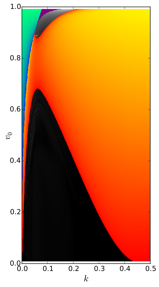
We now return to the collision of a single antikink with a homogeneous Robin boundary, and the way that this process interpolates between the integrable and limits. Many features of these collisions can be deduced from Fig. 8, a simple ‘snapshot’ plot of the field values at the boundary a fixed time after the initial impact. Two further plots in Fig. 9 summarise the results of a more-detailed analysis based on the numerical solution of the direct scattering problem for the final-state field, classifying the final states by their kink, antikink and high-energy breather content. Away from the integrable limits the final state always contains some radiation; and in various areas of the phase diagram (for example in parts of region VI) we also detected numbers of low-energy breathers. However the pattern of these low-energy breathers seems to be rather intricate, and hard to distinguish numerically from radiation, as the corresponding zeros of the Wronskian lie very near to the real axis. For this reason we will not discuss the low-energy breathers in detail below, but it would be of interest to return to their study in the future. Some typical examples of final states and the corresponding patterns of Wronskian zeros are shown in Fig. 10. Finally Fig. 11 illustrates some of the processes involved via spacetime plots of a variety of special cases.
I: Kink
II: Kink and antikink
III: High-energy breather
IV: High-energy breather and antikink
Va & Vb: Antikink
VI: None of the above.
a) , (region I)
b) , (region II)
c) , (region III)
d) , (region IV)
e) , (region Vb)

The Robin boundary for is the Neumann limit, and indeed we find that the incoming antikink is perfectly reflected into a kink without loss of energy, as shown in Fig. 11a. For slightly above zero it is still possible for the antikink to reflect into a kink, as shown in Fig. 11b, although some radiation is also generated, and energy is also left at the boundary since it ends up in the metastable vacuum. The region where this process occurs is labelled I of Fig. 9(a), and an approximation for its shape can be obtained by noting that the final state energy must be at least , where is the energy of the metastable vacuum as found in §3.1, and is the lower bound on the energy of the final-state kink. The initial energy is just that of an antikink with velocity , which is , where is the Lorentz factor. Some of this energy might be converted to radiation in the final state, so region I must lie within the region
| (23) |
The boundary derived from this expression is the dashed line in Fig. 9(a). It is a good approximation to the true boundary of region I while remains small, but clearly diverges from it at higher values. The reason is that after the initial collision, boundary oscillations can be excited, which in turn produce radiation. For higher energies and larger values of this effect becomes significant and the radiation produced is unaccounted for in our discussion. Compare, for example, the boundary oscillations for two different choices of and shown in Fig. 12.
The subsequent behaviour as increases further depends on the value of . If for the moment we restrict to then the first change, occuring as the energy bound just discussed comes into play, is that the reflected kink does not have enough energy to escape the boundary and instead recollides with it and reflects back as an antikink. This process is shown in Fig. 11c; it lies in region Va.
Increasing yet further brings us into region IV, where in addition to an antikink and some radiation a relatively high-energy (low frequency) breather is produced in the recollision, moving either slower than the antikink (Fig. 11d) or faster (Fig. 11l). At the left boundary of region IV the breather speed goes to zero and indeed in parts of region Va its presence can still be detected, trapped at the boundary as in Fig. 11e. This can be clearly seen in Fig. 14 where on the left hand edge of the plot (in Va) the boundary value of the field at the end of the simulation oscillates a great deal, corresponding to the trapped breather, while on the bottom right (in IV) it is always very close to zero as the breather has escaped. By contrast, as the right boundary of region IV is approached, the breather frequency goes to one and the breather energy goes to zero, marking the transition to region Vb where there is again just an antikink in the final state. The whole sequence of transitions is illustrated in Fig. 13(a).
For higher initial antikink velocities near to there is sufficient energy in the initial state to produce both a kink and an antikink: this occurs in region II, and is illustrated in Fig. 11f. The initial collision produces a kink with enough energy being left at the metastable boundary that some time later it decays with the emission of an antikink. As increases within region II, the speeds of the kink and antikink approach the same value, and the time between the release of the kink and antikink becomes smaller. Ultimately the kink and antikink ‘fuse’ into a very low frequency (loosely bound) breather as shown in Fig. 11g; this marks the transition from region II to region III, ending the sequence of transitions shown in Fig. 13(b). As increases further the frequency of this breather increases and its constituent kink and antikink become more tightly bound. We should also note that at the lower tip of region III the high energy breather produced in the initial collision can itself recollide with the Robin boundary, producing an extremely complicated pattern of results which we discuss in greater detail in §5.
To understand the transition from region III to region IV as increases even further, we note that (just as was the case for the emission of a kink) when only breathers are emitted the boundary is left in a metastable vacuum, with the field suffering some deformation near the boundary in order to satisfy the boundary condition. With increasing the barrier to the decay of this metastable vacuum decreases: in Fig. 11h (in region III) it is still high enough that although an antikink emerges it is unable to escape from the boundary, while in Fig. 11i (in region IV) it does escape, the boundary relaxing to the true () ground state.
As discussed above, increasing inside region VI increases the frequency of the emitted breather towards one. Its energy correspondingly decreases to zero, whereupon it disappears from the final state, leaving just a reflected antikink as in Fig. 11j. This marks the transition to the Dirichlet-like behaviour of region Vb.
Finally we note that it is also possible to find final-state breathers at lower energies, in region VI of Fig. 9(a), although the mechanism is somewhat different than that for region III. This process is shown in Fig. 11k : after initially rebounding the antikink fails to escape the boundary and instead forms a breather upon colliding with the boundary a second time. This breather appears to collide with the boundary multiple times and may eventually escape the boundary, as in Fig. 11k, or fail to do so over the time we evolve the sine-Gordon equation. This behaviour can be traced to the phase dependence of breather/boundary collisions and is discussed further at the end of §5. In this region we also often detect several very low energy breathers with frequency .
5 Resonance structure

Perhaps the most striking feature of our phase diagram is the ‘chaotic’ region shown in Fig. 14, which is reminiscent of the well-known patterns of resonance windows found in the non-integrable theory [17, 18, 19]. A window-like pattern of final velocities can also be seen in Fig. 15, a cross-section of this region at . Naively this might be surprising, as sine-Gordon kinks and antikinks lack the internal mode responsible for the resonance windows of the theory on the full line [17]. The critical distinction in the presence of a non-integrable boundary is that the initial antikink collision can create an intermediate breather, which does have an internal mode, and which furthermore can be attracted back towards the boundary to collide with it again. Several examples of this process, with dramatically different final states, are shown in Fig. 16.

The reason for the variety of outcomes in Fig. 16 is that the result of a breather colliding with a metastable Robin boundary is highly dependent on the point in the breather’s cycle at which it hits the boundary. As shown in Fig. 17, simply changing the initial phase of the breather can create a completely different final state after collision with the boundary. In Fig. 17a the breather fissions into an antikink and a boundary breather, while Fig. 17c has a similar outcome but only after an intermediate breather is created and recollides with the boundary. Fig. 17d shows the breather being reconfigured into a breather of lower mass and higher speed, and Fig. 17b shows this outcome happening via an intermediate antikink and breather.

This strong phase dependence suggests that the breather and antikink resonance windows exemplified in Fig. 15 occur when the frequency and initial phase and velocity of the intermediate breather are such that it recollides with the boundary at exactly the ‘right’ phase to produce an antikink and/or breather which escapes the boundary. Of course for our model it is the initial antikink speed, , and the boundary parameter, , which indirectly controls all the characteristics of the intermediate breather.
Let us consider moving between these resonance windows in more detail for the specific case where , as shown in Fig. 15. Starting at a label 1 in Fig. 15 the intermediate breather collides with the boundary and produces a breather which then escapes the boundary, as in Fig. 16a. As increases first an antikink is produced in addition to the breather, shown in Fig. 16b and corresponding to label 2 in Fig. 15. Then as the breather speed decreases it becomes trapped at the boundary as in Fig. 16c. Eventually the antikink fails to escape the boundary, which marks label 3 in Fig. 15 and the beginning of the indeterminate region which, as we see in Fig. 16d, e and f is due to multiple intermediate antikinks and breathers scattering off the boundary. Of course each successive intermediate breather produced will have its own resonance windows that may allow a breather or antikink to escape. So the final result we see for the indeterminate regions in Fig. 15 is a product of one or more of these nested resonance windows, giving these regions their chaotic appearance. As continues to increase there will eventually come a point where the phase of the intermediate breather as it collides with the boundary cycles back to its original value where a breather is produced. For example, in Fig. 16g the breather has undergone an additional full cycle in its oscillation compared to Fig. 16a and the final states are quite similar.
For a sufficiently high (the precise value being dependent upon ) the breather formed after the initial collision has enough energy to escape the boundary in the first instance, as in the rest of region III in Fig. 9(a).
For sufficiently low (again, depending on ) an antikink with (in region IV) or without (in region V) a breather is produced. Comparing Fig. 11l and Fig. 11e to Fig. 16b and Fig. 16c suggests that this transition to regions IV and V can be interpreted as the intermediate breather becoming very short lived and colliding with the boundary before oscillating a full cycle. Because the breather is so short-lived it appears very much like a short-lived kink. This coincides with the interpretation discussed in §4 that as is increased from region I there is an intermediate kink which exists for a progressively shorter time. For example, compare the progression from Fig. 11c to d to e.
Finally, a basic explanation for the behaviour observed in region VI and exemplified in Fig. 11k, where the recollision of an intermediate antikink creates a breather which may collide with the boundary multiple times before escaping, is now apparent. The breather will only escape when its phase as it hits the boundary is such that after the collision it has a mass and speed that allows it to escape the boundary, schematically similar to the case shown in Fig. 17d. We therefore expect this region to exhibit a similarly chaotic pattern of breather escapes as was seen in the lower portion of region III for antikink escapes. Note though that the total energy available available to the breather is less than the escape energy of an antikink, since the breather itself was formed by a returning antikink. For this reason any chaotic patterns will only be visible in the breather spectrum, making them much harder to see than in region III. Further (and higher-precision) study will be required before the full picture in this region is clear.
6 The Robin boundary with
Here we will make some brief remarks on the case when . It is known that the integrable boundary, Eq.(2), with is unstable for since the boundary potential, , then allows for a family of degenerate zero energy solutions [20]. For example, with an initial condition of , a kink may be emitted without any loss of energy.
The Robin boundary appears to exhibit similar instabilities. For the incoming antikink is converted into a kink but we observed that for additional kinks are produced. This threshold can be approximated by noting that if then so that the energy required to release the additional kink is offset by the energy released due to the boundary moving up . If this inequality is satisfied then so will for which allows for an infinite number of kinks to be produced from the boundary.
As k becomes increasingly negative the numerical simulation becomes unstable with even the slightest increase in the value of the field at the boundary from its initial value of zero causing the field at the boundary to blow up to infinity.
7 Conclusions
We have examined the wide range of processes and outcomes arising from the collision of an antikink solution to the sine-Gordon equation with a non-integrable Robin boundary. An important feature of our analysis was the numerical implementation of the direct scattering transform which enabled us to disentangle the excitation content of the final state in an efficient manner. Even though integrability is only broken at one point, the structure turned out to be very rich: Figs. 8 and 9 summarise the broad features, while Figs. 14 and 15 reveal a complicated finer structure. In the integrable Neumann and Dirichlet limits the results of the collisions approach the exact solutions for these boundaries: close to the antikink reflects into a kink (region I), while for large the antikink retains its character as an antikink (region Vb). Away from these limits the non-integrability of the boundary allows the production of a kink and an antikink (region II), high energy breathers (region III), an antikink accompanied by a breather (region IV), or the annihilation of the initial antikink into either radiation or low energy breathers (region VI). The most exotic features observed were the resonance structures of Fig. 14, and their origin was traced to the phase dependence of the recollision of intermediate breathers with the boundary.
While an approximation to the boundary of region I was given, our discussion was largely phenomenological and we have not found analytical arguments for the shapes of the other regions. Progress in this area would appear to require a greater quantitative understanding of how the antikink initially collides with the boundary. For example, deriving the shape of region VI would require a model of how much energy the incoming antikink loses in its initial collision with the boundary for a given and . This would determine whether the antikink has sufficient energy to escape the boundary. In the case of the model on the full line a similar style of analysis has yielded considerable insights [17, 18, 19], so this should be a promising avenue for further work.
Perhaps the most interesting result was the intricate resonance structure seen in Fig. 14, which we traced to the phase dependence of the recollision of intermediate breathers with the boundary. This behaviour is clearly deserving of a more detailed analysis. Such resonance phenomena greatly increase sensitivity not only to initial conditions but also to numerical error, and while we tried to keep these issues under control by varying the time and space steps in our simulations, a closer examination of the patterns of resonance windows using more sophisticated numerical methods would be very valuable, both in the regions of windowed antikink escape shown in Fig. 14, and in also in the portions of region VI which appear to have a similar pattern of escape and non-escape, but for breathers rather than antikinks. Work on this question is in progress. To make further analytical headway, a better understanding of the way that the initial antikink velocity combines with the boundary parameter to determine the characteristics of the first intermediate breather, and how these in turn affect its subsequent recollision with the boundary, will be required. A first step is therefore likely to involve a more-detailed and higher-precision study of how a breather with a given initial phase, frequency and velocity collides with the various metastable Robin boundaries.
It would also be interesting to see whether the fact that the model remains integrable away from the boundary can be exploited in a more direct way, possibly within the framework of the Fokas (or unified) method. With respect to integrable PDEs on the half line this can be viewed as a generalisation of the inverse scattering transform [21, 22].
Specialised to the sine-Gordon equation, the Fokas method requires not only the initial data and , but also the, most likely unknown, boundary data and . A key component in this method is therefore the so-called ‘global relation’, an equation relating the spectral functions associated with the initial data and the boundary data. If one considers a boundary problem where is a known function of time then it is possible to derive a ‘Dirichlet to Neumann map’ and obtain a perturbative expansion for the unknown [23, 24]. An analogous procedure can be carried out when is known and unknown. Alternatively, for certain boundary conditions termed ‘linearizable’ there is an additional symmetry of the Lax pair eigenfunction which makes it possible to solve the global relation algebraically, bypassing the need for a perturbative solution for . For sine-Gordon the known linearizable boundary conditions are nothing but the integrable boundaries of Eq.(2) [5].
However, the sine-Gordon equation with a Robin boundary of the type we have considered does not fit into either of these cases. That is to say it is not linearizable and we do not know a priori or for . At present we are unaware of a scheme that would allow us to apply the Fokas method given only a relationship between and such as, . Given the complexity of the behaviour that we have observed, this would seem to present an interesting challenge for the wider applicability of the method.
Another direction for future work is to investigate whether the classical phenomena that we have found have their counterparts in the corresponding boundary quantum field theories. There has been a certain amount of work treating non-integrable bulk quantum field theories as deformations of integrable theories (see for example [25]), and it would be interesting to apply similar ideas to problems where integrability is instead broken just at a boundary. In particular, since all excitations are asymptotically far from that boundary, one would expect the space of in- and out- states to be exactly the same as for the integrable theory. This major simplification should enable significantly more progress to be made than in previously-studied bulk examples.
Finally, and returning to classical considerations, we note that the method for numerically obtaining the soliton and breather content after collision is not limited to the sine-Gordon equation and could easily be extended to any integrable model that permits a solution via the inverse scattering transform with any non-integrable boundary or even defect. The analysis of other boundary or defect models may well benefit from the additional information this provides.
Acknowledgements
We wish to thank Vincent Caudrellier and Ed Corrigan for helpful comments and encouragement during the later stages of this work, and Giuseppe Mussardo for useful correspondence. PED would also like to thank Tomasz Romanczukiewicz and Yasha Shnir for collaboration on related topics. PED was supported in part by an STFC Consolidated Grant, ST/L000407/1, and also by the GATIS Marie Curie FP7 network (gatis.desy.eu) under REA Grant Agreement No 317089. RP was supported by an EPSRC vacation bursary while the majority of this research was carried out and gratefully acknowledges the support of an EPSRC studentship at present.
References
References
- [2] R.F. Bikbaev and V.O. Tarasov. A nonhomogeneous boundary value problem on a semiaxis and on an interval for the sine-Gordon equation. St. Petersburg Math. J., 3(4):775–789, 1992.
- [3] S. Ghoshal and A. Zamolodchikov. Boundary S-matrix and boundary state in two- dimensional integrable quantum field theory. Int. J. Mod. Pys. A, 9:3841–3886, 1994.
- [4] A. MacIntyre. Integrable boundary conditions for classical sine-Gordon theory. J.Phys. A, 28:1089–1100, 1995.
- [5] A.S. Fokas. Linearizable initial boundary value problems for the sine-Gordon equation on the half-line. Nonlinearity, 17(4):1521–1534, 2004.
- [6] H. Saleur, S. Skorik and N.P. Warner. The boundary sine-Gordon theory: classical and semi-classical analysis. Nuclear Physics B, 441(3):421–436, 1995.
- [7] O.H. Olsen and M.R. Samuelsen. Fluxon propagation in long Josephson junctions with external magnetic field. Journal of Applied Physics, 52(10):6247–6251, 1981.
- [8] P. Dorey, A. Halavanau, J. Mercer, T. Romanczukiewicz and Y. Shnir. Boundary scattering in the model. 2015. ArXiv: 1508.02329
- [9] L.A. Takhtadzhyan and L.D. Faddeev. Essentially nonlinear one-dimensional model of classical field theory. Theor. and Math. Phys., 21(2):1046–1057, 1974.
- [10] M. Ablowitz and H. Segur. Solitons and the inverse scattering transform. SIAM, 1981.
- [11] M.G. Forest and D.W. McLaughlin. Spectral theory for the periodic sine-Gordon equation: A concrete viewpoint. Journal of Mathematical Physics, 23(7):1248–1277, 1982.
- [12] M. Dellnitz, O. Schütze and Q. Zheng. Locating all the zeros of an analytic function in one complex variable. J. Compu. and App. Math., 138(2):325–333, 2002.
- [13] E. Jones, T. Oliphant, P. Peterson and others. SciPy: Open Source Scientific Tools for Python. URL: http://www.scipy.org/
- [14] N. Manton and P. Sutcliffe. Topological Solitons. CUP, 2004.
- [15] M. Nishida, Y. Furukawa, T. Fujii and N. Hatakenaka. Breather-breather interactions in sine-Gordon systems using collective coordinate approach. Phys. Rev. E, 80(3):036603, 2009.
- [16] S.V. Dmitriev, Y.S. Kivshar and T. Shigenari. Fractal structures and multiparticle effects in soliton scattering. Phys. Rev. E, 64(5):056613, 2001.
- [17] D.K. Campbell, J.F. Schonfeld and C.A. Wingate. Resonance structure in kink - antikink interactions in theory. Physica D, 9:1, 1983.
- [18] P. Anninos, S. Oliveira and R.A. Matzner. Fractal structure in the scalar theory. Phys. Rev. D 44:1147, 1991.
- [19] R. Goodman and R. Haberman. Chaotic scattering and the -bounce resonance in solitary wave interactions. Phys. Rev. Lett. 98:104103, 2007.
- [20] A. Fujii and R. Sasaki. Boundary effects in integrable field theory on a half line. Prog. Theor. Phys., 93(6):1123–1133, 1995.
- [21] B. Pelloni. Advances in the study of boundary value problems for nonlinear integrable PDEs. Nonlinearity, 28:R1–R38, 2015.
- [22] A.S. Fokas. A unified approach to boundary value problems. SIAM, 2008.
- [23] A.S. Fokas. The generalized Dirichlet to Neumann map for certain nonlinear evolution PDEs. Communications on Pure and Applied Mathematics, 58(5):639–670, 2005.
- [24] G. Hwang. The Fokas method: The Dirichlet to Neumann map for the sine-Gordon equation. Studies in Applied Mathematics, 132:381–406, 2014.
- [25] G. Delfino, G. Mussardo and P. Simonetti. Nonintegrable quantum field theories as perturbations of certain integrable models. Nucl. Phys. B, 473:469, 1996.