Approximately Truthful Multi-Agent Optimization Using Cloud-Enforced Joint Differential Privacy
Abstract
Multi-agent coordination problems often require agents to exchange state information in order to reach some collective goal, such as agreement on a final state value. In some cases, it is feasible that opportunistic agents may deceptively report false state values for their own benefit, e.g., to claim a larger portion of shared resources. Motivated by such cases, this paper presents a multi-agent coordination framework which disincentivizes opportunistic misreporting of state information. This paper focuses on multi-agent coordination problems that can be stated as nonlinear programs, with non-separable constraints coupling the agents. In this setting, an opportunistic agent may be tempted to skew the problem’s constraints in its favor to reduce its local cost, and this is exactly the behavior we seek to disincentivize. The framework presented uses a primal-dual approach wherein the agents compute primal updates and a centralized cloud computer computes dual updates. All computations performed by the cloud are carried out in a way that enforces joint differential privacy, which adds noise in order to dilute any agent’s influence upon the value of its cost function in the problem. We show that this dilution deters agents from intentionally misreporting their states to the cloud, and present bounds on the possible cost reduction an agent can attain through misreporting its state. This work extends our earlier work on incorporating ordinary differential privacy into multi-agent optimization, and we show that this work can be modified to provide a disincentivize for misreporting states to the cloud. Numerical results are presented to demonstrate convergence of the optimization algorithm under joint differential privacy.
I Introduction
Multi-agent optimization problems have found applications in a range of research areas, including power systems in [17], machine learning in [3], sensor networks in [5], and robotics in [19]. Solutions to some problems in these applications rely on the implicit assumption that all agents share correct, truthful information with others in a network. However, one can envision a scenario in which deceitful agents do not honestly share their data, instead sharing false information that will skew the behavior of the system in their favor. For example, a homeowner connected to a smart power grid may report a false value for his or her power usage in order to save money. This paper considers optimization problems with agents that may be intentionally deceitful for their own benefit, and it provides a method for disincentivizing untruthful behavior when teams of agents are collectively optimizing.
We reduce the incentive to share false information by using joint differential privacy, defined in [13], to limit the possible decrease in cost an agent can achieve through intentionally misreporting its state. Joint differential privacy adds noise to reduce the ability of an agent to benefit from reporting false information, and was first introduced for this purpose in [13] to promote truthful sharing of information by the players in a class of games. This work was applied specifically to optimization problems arising from distributed electric vehicle charging in [11], as well as to linearly separable optimization problems in [12].
The developments in this paper differ from those in [11] and [12], as well as some other work on private optimization, e.g., [10], in two key ways. First, the work in [11], [12], and [10] uses differential privacy as it was originally defined in [7] to keep some static object, such as a constraint function, private. Our work focuses on trajectory-level privacy for state trajectories that are dynamically generated as an optimization algorithm is executed. In applications such as phase synchronization in smart power grids, each iterate of an optimization algorithm corresponds to a physical state at some point in time, and an agent’s contribution to the optimization process is its whole state trajectory. Applying joint differential privacy in such applications should therefore be done at the trajectory level, and implementing joint differential privacy for trajectory-level data is most naturally done using the dynamical systems formulation of differential privacy. Therefore, this paper uses trajectory-level privacy as defined in [15], rather than privacy for databases as in [7].
This form of privacy is not only better suited to the applications of interest, but also allows privacy guarantees to hold across infinite time horizons which, in many cases, cannot be attained using privacy for databases. To our knowledge, this paper is the first use of joint differential privacy at the trajectory level. The second key difference between the existing literature and this paper is the class of optimization problems solved. We apply joint differential privacy in a general multi-agent nonlinear programming setting, incorporating non-separable functional constraints that are also possibly nonlinear, which differs from work done in [11], [12], and [10] where either linear or affine constraints are considered.
To solve such problems, a cloud computer is added to the team of agents to serve as a trusted central aggregator, also sometimes called a “curator” in the privacy literature. This architecture was previously used for privately solving multi-agent nonlinear programs in [9], in which honest agents seek to protect sensitive data from eavesdroppers via ordinary differential privacy. The work in [16] suggests that any differential privacy implementation provides some disincentive against untruthful information sharing, and the current paper uses the notion of joint differential privacy to formally provide this guarantee in the framework developed in [9]. Accordingly, the technical novelty of this paper is not in the algorithm used to solve problems, but in the theoretical performance guarantees that are provided using this framework; the work in [9] focuses exclusively on protecting sensitive data, but the current paper focuses on the problem of preventing untruthful behavior by the agents. The technical contribution of this paper thus consists of adapting our existing privacy framework to the problem of incentivizing truthful behavior by the agents, and quantifying the extent to which any agent can benefit from untruthful behavior.
Several existing approaches use behavioral analysis to identify untruthful agents, including those in [4] and [8]. In this paper, an agent’s local state updates rely on a local objective function and local constraint set that are considered sensitive, and therefore these local data are not shared with any other agent. As a result, the correct next value of an agent’s state is only known to that agent, and a behavioral analysis approach cannot be used here because no outside observer can determine what any agent’s future states should be. Rather than detecting untruthful behavior, this paper seeks to prevent it outright by reducing the incentive to share untruthful information via joint differential privacy. The principle underlying this application of joint differential privacy is that adding noise to the system can make each agent’s cost insensitive to changes in the agent’s state trajectory. The amount of noise added must be calibrated to the system in order to dilute the effect of an agent reporting an untruthful state to the cloud, and this paper presents this calibration for a general multi-agent nonlinear program in terms of constants pertaining to the problem.
The problems considered consist of a collection of agents, each with a local objective function and local set constraint, and ensemble state constraints that jointly constrain the agents. A primal-dual approach is used, in which the agents update their own states, which are the problem’s primal variables, and the cloud updates the problem’s dual variables. Naturally, the constraints in this problem will usually lead to higher costs for each agent than a comparable unconstrained problem. As a result, some of the agents may wish to skew the constraints in their favor. One way they may do so is by reporting false state information to the cloud in order to loosen the constraints’ effects on their on their own states, thereby giving the untruthful agents a lower cost. This manipulation of the constraints will result in an unequal distribution of the burden of these constraints by tightening them on honest agents. Therefore, this form of untruthful behavior is disincentivized using joint differential privacy.
The rest of the paper is organized as follows. Section II provides the necessary optimization background, the structure of communications in the system, and formally states the joint differentially private optimization problem that is the focus of the paper. Then, Section III reviews joint differential privacy, and Section IV presents the proposed joint differentially private algorithm. Next, Section V proves the main result of the paper on limiting an agent’s incentive to misreport its states to the cloud. Section VI then presents simulation results and Section VII concludes the paper.
II Background on Optimization and Problem Statement
This section presents the multi-agent optimization problem of interest and an optimization algorithm that will later be used to solve a joint differentially private version of this problem. This section also describes the cloud-based architecture used to solve this problem. Throughout the paper, denotes the partial derivative with respect to , and denotes the partial derivative of the function with respect to .
II-A Optimization Problem Formulation
Consider a problem consisting of agents indexed over . Agent has state with and a local set constraint of the form . The diameter of is denoted by . Agent also has a local objective function depending only upon its own state. Agent ’s local data are subject to the following assumption.
Assumption 1
For all , is and convex in , and is non-empty, compact, and convex.
Assumption 1 implies that is Lipschitz and its Lipschitz11 1 All Lipschitz constants in this paper are with respect to the metric induced by the -norm. constant is denoted by . In particular, Assumption 1 allows for convex polynomial objectives and box constraints, which are common in multi-agent optimization problems. Both and are considered sensitive information and are therefore not shared with the other agents or with the cloud. For simplicity of notation, define the set , where . The agents’ individual set constraints require , where is the ensemble state vector of the network, defined as , and where Assumption 1 provides that is non-empty, compact, and convex.
The agents are together subject to global inequality constraints , where . The functional constraints in are subject to the following assumption.
Assumption 2
- i.
For all , the constraint is and convex in .
- ii.
There exists a point such that .
Assumption 2.i. admits a wide variety of constraint functions, e.g., any convex polynomials. Assumption 2.ii. is known as Slater’s condition, e.g., Assumption 6.4.2 in [2], and, in conjunction with Assumption 2.i., guarantees that strong duality holds. Assumption 2 implies that and each are Lipschitz. Their Lipschitz constants are denoted by and , respectively.
Summing the per-agent objective functions gives the ensemble objective , which is and convex in because of Assumption 1. Together , , and comprise the following ensemble-level optimization problem.
Problem 0
(Preliminary; no joint differential privacy yet)
| minimize | ||||
| subject to | ||||
We now detail how to solve Problem 0 in the cloud-based system, and then give a unified problem statement, including incentivizing truthful behavior, in Problem 1 below.
The Lagrangian associated with Problem 0 is
| (1) |
where is the dual vector associated with Problem 0 and denotes the non-negative orthant of Seminal work of [14] shows that a point is a solution to Problem 0 if and only if there exists a point such that is a saddle point of . This saddle point condition can be compactly expressed by requiring
| (2) |
and an optimal primal-dual pair exists under Assumptions 1 and 2.
For the forthcoming optimization algorithm, Equation (2) is used to define an upper bound on the norm of , stated in the following lemma. It uses the Slater point from Assumption 2.ii. and any lower bound on over , denoted , which exists under Assumption 1.
Lemma 1
For a saddle point of ,
| (3) |
Proof: See Section II-A in [9].
Using the fact that a saddle point of provides a solution to Problem 0, the remainder of the paper focuses on finding such saddle points. The algorithm used for this purpose includes an iterative Tikhonov regularization with an asymptotically vanishing stepsize, and was stated in [1] for deterministic variational inequalities and later in [18] for stochastic problems. To help describe the communications and computations in the cloud-based system, we provide the general deterministic form of this algorithm now, though in Section IV stochasticity is introduced when the algorithm is made joint differentially private. The saddle-point finding algorithm uses the coupled update equations
| (4a) | ||||
| (4b) | ||||
where and are the Euclidean projections onto and , respectively. This update law will be referred to as Update (4). Here, is a stepsize and is the regularization parameter, and the values of both will be provided in Theorem 1 in Section IV.

II-B Optimizing via the Cloud
We now elaborate on the cloud-based architecture to be used and the means of executing Update (4) on the cloud and agents. To enforce joint differential privacy, the agents do not directly share any information with each other. Instead, the agents route messages through a trusted cloud computer which aggregates all states in the network, performs computations involving these states, and makes the results of these computations joint differentially private before sending them to the agents.
Splitting Equation (4a) into each agent’s states gives the update
| (5) |
for agent , where expanding the term containing gives
| (6) |
Importantly, the right-hand side of Equation (6) contains two terms which agent cannot compute on its own: , because it is a function of every state in the network, and , because its update law relies on , which is also a function of every state in the network. For this reason, the cloud computer is used to compute and for each at all timesteps .
Four actions occur within timestep . First, agent sends to the cloud and the cloud assembles the ensemble state vector . Second, the cloud computes for every . Third, the cloud sends to agent . Fourth, the cloud computes and simultaneously agent computes , and then this process repeats. This exchange of information is depicted in Figure 1. In the upper-left panel of Figure 1, agents through report their actual state to the cloud, while agent misreports its state to the cloud by sending some instead of . The arrows connecting boxes indicate how misreported states propagate through the system, eventually affecting all agents’ states. The cloud’s computations in Steps 2 and 4 will be modified in Section III to introduce joint differential privacy, though the overall communications structure will remain the same.
To reflect that agent receives the vector from the cloud without knowing or individually, agent ’s update law is rewritten as
| (7) |
where . As in Equation (4b), the cloud computes the dual update according to
| (8) |
II-C Full Problem Statement
We now state the algorithm that will be used throughout the remainder of the paper. Below that, we identify the potential for misreporting states in this algorithm and state the problem that is later solved using joint differential privacy.
Algorithm 1
Step 0: For all , initialize agent with , , , , and .
Initialize the cloud with , , , , and . Let the cloud compute
before the system begins optimizing. Set .
Step 1: For all , the cloud computes and sends it to agent .
Step 2: Agent computes
| (a) |
and sends a state value to the cloud.
Step 3: The cloud computes
| (b) |
Step 4: Set and return to Step 1.
In Step of Algorithm 1, agent may report a false state value to the cloud, sending some . This is the misreporting behavior that this paper seeks to prevent using the cloud. The only influence the cloud has upon agent is through , and therefore the cloud must compute in a way that incentivizes agent to honestly report its state. The incentivization of this behavior is stated as Problem 1 below, and the remainder of the paper focuses on solving Problem 1.
Problem 1
Execute Algorithm 1 with the cloud computing in a way that incentivizes agent to honestly report in Step , while still converging to a minimum.
It is assumed that each agent ultimately wants the constraints to be satisfied, as would be the case when corresponds to some mission-critical conditions that must be satisfied by the agents. However, an agent may wish to reduce the impact has upon its own state in order to reduce its cost. One way of affecting for this purpose is by reporting false states to the cloud over time; because all agents want to be satisfied, a misreporting agent will still use from the cloud in its state updates, but an agent can substantially influence these messages for its own benefit through misreport. In response to misreported states, other agents’ messages from the cloud in Update (4) will be affected in a way that compensates for agent ’s false reported states, thereby resulting in an unfair distribution of the burden of .
This behavior cannot be detected by the other agents or the cloud because only agent knows and , making no other entity in the network capable of determining what agent ’s state should be (cf. Equation (4a)). Therefore, rather than detecting manipulation of , we seek to prevent this behavior. Joint differential privacy provides a framework for incentivizing truthful sharing of information and it is used here to prevent the agents from manipulating .
Because agents are opportunistic but not malicious, they may send untruthful states to the cloud, but they will not send states that harm the system or prevent convergence of Algorithm 1. As a result, a misreported state trajectory will have some relationship to an agent’s true state trajectory and this relationship is used in defining adjacency of signals in our joint differential privacy implementation. The next section details the manner in which noise is added to using joint differential privacy, and Section IV shows that this noise still allows for Algorithm 1 to reach a minimum.
III Joint Differential Privacy
This section recalls necessary details from both ordinary differential privacy and joint differential privacy. Then it presents the joint differential privacy mechanism that will be implemented on the preceding cloud architecture. It is critically important to note that while this section discusses privacy, the ultimate goal is to apply joint differential privacy to induce truthful sharing of states. All of the content on privacy in this section should therefore be understood as making progress toward inducing truthful behavior.
III-A Differential Privacy Background
Differential privacy as described in [7] was originally designed to keep individual database entries private whenever a database is queried, and this is done by adding noise to the responses to such queries. This idea was extended to dynamical systems in [15] in order to keep inputs to a system private from anyone observing the outputs of that system. It is the dynamical systems notion of differential privacy that is used below.
The key idea behind differential privacy is that noise is added to make “adjacent” inputs produce “similar” outputs, and these notions are made rigorous below. As above, let there be users, with the user contributing a signal . The space is the space of sequences of -vectors in which every finite truncation of every element has finite -norm. More explicitly, with denoting the element of the signal , define the truncation operator according to
| (10) |
Then if and only if for all . The full input space is then defined by the Cartesian product . This paper focuses on the case where for all .
To formalize the notion of adjacency of inputs in , we define a binary, symmetric adjacency relation , which is parameterized by and an index . Its definition uses the notation . The adjacency relation takes the form and has the following definition, as stated in [15].
Definition 1
Two inputs , satisfy for some if and only if . The signals and are then said to be adjacent with respect to agent . If is arbitrary, the relation is used, and and are simply called adjacent.
This section maintains use of the symbol for system inputs (rather than as will be in subsequent sections) to maintain continuity with the references cited here for private dynamical systems.
Inputs from are assumed to pass into a causal, deterministic system , which produces outputs in . To define when two outputs are “similar,” the notion of a mechanism is used. In the context of private dynamical systems, a mechanism is a means of adding noise to an otherwise deterministic system to provide privacy to that system’s inputs. Formally, for a fixed a probability space , a mechanism is a map of the form
| (11) |
The mechanism must provide differential privacy to its input trajectories, which fundamentally means that the output of should be insensitive to changes in its inputs. Differential privacy captures this notion by requiring that, whenever holds, the probability distributions of and satisfy
| (12) |
for all in an appropriate -algebra.
Using a result from the literature, we now state a finite-time criterion which holds if and only if keeps entire trajectories private. Below, the notation is used to refer to the first entries of .
Lemma 2
Let be given. For a dynamical system, a mechanism is -differentially private if and only if, for all , satisfying and for all times ,
| (13) |
where is the Borel sigma-algebra on and is the dimension of the output space.
Proof: See Lemma 2 in [15].
In Lemma 2, the value of determines the level of privacy afforded to the input signals, and decreasing its value leads to improved privacy at the cost of adding higher variance noise. Typical values of in the literature range from to .
III-B Joint Differential Privacy
We now elaborate on the application of joint differential privacy to Problem 1. To promote truth-telling behaviors, limits are imposed on the ability of any agent to reduce its cost by reporting a false state trajectory to the cloud. These limits are enforced using joint differential privacy, which is a relaxation of ordinary differential privacy for use in multi-agent systems, and it will be shown that this framework is sufficient for the goal of reducing an agent’s ability to benefit from misreporting its state. For joint differential privacy, the “system” of interest is comprised by the computations the cloud carries out in accordance with Update (4), and this point is discussed further below. For now it suffices to point out that the output of this system is a tuple of private forms of all ’s. Denoting the private form of by (whose exact form will be given later), the output of the cloud at time is denoted by
| (14) |
Let denote a mechanism for joint differential privacy and let denote the same mechanism with the output removed, i.e., the output of is
| (15) |
A mechanism is joint differentially private if, for any , preserves differential privacy for inputs adjacent with respect to . Joint differential privacy for databases has been defined in [13], though, to our knowledge, it has not yet been used for dynamical systems. Using Lemma 2 in [15], the following lemma states a finite-time criterion for trajectory-level joint differential privacy.
Lemma 3
(Joint differential privacy for dynamical systems) Let the privacy parameter be given and let be a mechanism whose output is an -tuple. Then is -joint differentially private if and only if, for any , for all satisfying , all times , and all , satisfies
| (16) |
where is the Borel sigma-algebra on .
Joint differential privacy guarantees that when agent ’s input changes by a small amount, the outputs corresponding to other agents do not change by much. A useful characteristic of both ordinary and joint differential privacy is their resilience to post-processing, which guarantees that post-hoc transformations of private data cannot weaken the privacy guarantees afforded to that data. This result is formalized below.
Lemma 4
(Resilience to post-processing; [6, Proposition 2.1]) Let be an -differentially private mechanism and let be a function such that the composition is well-defined. Them is also -differentially private.
III-C The Laplace Mechanism
To enforce differential privacy for a particular choice of , noise must be added somewhere in the system, and the distribution of this noise must be determined. One common mechanism in the literature draws noise from the Laplace distribution, used in both [7] and [15], and this mechanism is used to provide -joint differential privacy. To define this mechanism, the notion of the sensitivity of a system is now introduced.
Definition 2
The sensitivity of a deterministic, causal system is defined as
The Laplace mechanism is stated in terms of the sensitivity of a system. Below, the notation denotes a scalar Laplace distribution with mean zero and scale parameter , i.e.,
| (17) |
Lemma 5
(Laplace mechanism; [15, Theorem 4]) Let be given. The Laplace mechanism defined by
| (18) |
with is -differentially private for , with the dimension of the output space of the system.
IV Optimizing Under Joint Differential Privacy
In this section, the privacy results in Section III are applied to Problem 1, and Algorithm 1 is made joint differentially private. Formally, and are treated as memoryless dynamical systems, and joint differential privacy is used to ensure that they keep the agents’ state trajectories, which are the inputs to these systems, private.
IV-A Stochastic Optimization Algorithm
From Lemma 3, we see that enforcing joint differential privacy for the states in the network requires that the cloud make private before it is sent to agent . To make private, noise can be added to it directly and this is done below. To make private, we use the fact that computing relies on , and add noise to make private. Then computing is joint differentially private by the post-processing property in Lemma 4. Similarly, if the noisy forms of both and are joint differentially private, their product is as well, again by Lemma 4. Adding noise in this way, Algorithm 1 is modified to state the joint differentially private optimization algorithm below.
Algorithm 2
Step 0: For all , initialize agent with , , , , and .
Initialize the cloud with , , , , and . Let the cloud compute
before the system begins optimizing. Set .
Step 1: For all , the cloud computes
and sends it to agent .
Step 2: Agent computes
| (a) |
and sends a state value to the cloud.
Step 3: The cloud computes
| (b) |
Step 4: Set and return to Step 1.
To solve Problem 1, Algorithm 2 must implement joint differential privacy using the noise terms and , while still converging to a minimum. The following theorem gives conditions on and each under which convergence to a minimum is guaranteed. Then Theorem 2 shows that joint differential privacy is achieved under these conditions, and Section V shows that each agent’s incentive for misreport is indeed limited due to joint differential privacy.
Theorem 1
Let denote the least-norm saddle point of . Algorithm 2 satisfies
| (19) |
if i. and have zero mean for all
ii. and , where , , , and .
Proof: See [18, Theorem 6].
It remains to be shown that Condition i of Theorem 1 can be satisfied when joint differential privacy is implemented, and this is done next.
IV-B Calibrating Noise for Joint Differential Privacy
Here the systems being made private are and , and the mechanisms acting for joint differential privacy add noise to when computing and add noise to when computing . It was shown in Section III that the noise added in Algorithm 2 will enforce -joint differential privacy as long as it has large enough variance. To determine the variance of noise that must be added by the Laplace mechanism, bounds are derived on the sensitivity of each and below.
Lemma 6
For the relation , the sensitivities of and satisfy and .
Proof: See [9].
Using Lemmas 5 and 6, we see that if with and with for all , then all states are afforded (ordinary) -differential privacy in Algorithm 2. It turns out that this privacy and its resilience to post-processing imply that -joint differential privacy holds as well, which is stated formally in the following theorem.
Theorem 2
Proof: We examine for an arbitrary whose output at time is
| (21) |
Examining some , the output is
| (22) |
In light of the fact that with , we see that keeps -differentially private. Similarly, keeps -differentially private because and . By Lemma 4, the product keeps -differentially private because it is the result of post-processing two differentially private quantities. By the same reasoning,
| (23) |
simply post-processes differentially private information. From Lemma 3 we conclude that is -joint differentially private.
The next section describes the application of this mechanism to inducing approximately-truthful behavior in multi-agent optimization through the computation of -approximate minima.
V Computing -approximate Minima
This section presents the main result of the paper: joint differential privacy results in there being only minimal incentive for an agent to misreport its state to the cloud. Toward showing this result, a uniform upper bound on over is first presented.
Lemma 7
Let denote a Slater point for . Then for all , for all , where .
Proof: Using the Mean-Value Theorem and the Cauchy-Schwarz inequality, we have
| (24) | ||||
| (25) |
for some . The result follows by bounding by and bounding by .
The next lemma bounds the difference in at points along two feasible state trajectories for agent .
Lemma 8
For any and any time , one finds
| (26) |
Proof: Using the Lipschitz property of ,
| (27) |
On the other hand, the triangle inequality gives
| (28) |
where the second inequality follows from Lemma 7.
The main result of the paper is now presented. Below, each expected value is over the randomness introduced by the mechanism . For clarity, this theorem tracks the state agent has reported to the cloud and the state trajectory of every other agent. The notation is used to denote agent ’s cost at time when agent has reported the trajectory to the cloud and every other agent has followed the trajectory . The symbol is always used as the argument to because always depends on the true state of agent , not the state it reports.
Theorem 3
Suppose Assumptions 1 and 2 hold. Let the agents and cloud execute Algorithm 2 with the cloud implementing the mechanism . Then for , all agents sharing their true states in Algorithm 2 results in a -approximate minimum. In particular, at all times and for any state trajectories satisfying , we have
| (29) |
where , and where is a misreported state trajectory from agent .
Proof: From Lemma 8 we have
| (30) |
Using Theorem 2 and the definition of -joint differential privacy we find
| (31) |
which we substitute into Equation (30) to find
| (32) |
Using for gives
| (33) |
were we apply Lemma 7 to get
| (34) |
A second application of Lemma 8 gives
| (35) |
and substituting this inequality into Equation (34) gives
| (36) |
as desired.
While the term in is a feature of the problem itself, the term results directly from the untruthfulness of agent , and it is precisely this term which can be influenced using the privacy parameter , allowing a network operator to directly counteract the influence of false information. Of course, shrinking requires that more noise be added which, in general, degrades performance in the system. One must therefore balance the two objectives of incentivizing truthful information sharing and system performance based upon the needs in a particular application.
VI Simulation Results
A simulation was run consisting of agents each with , and constraints. The constraint for all , and , for all ; the value of each can be found in Table I. The constraints used were
| (37) |
The value was used for adjacency and the privacy parameter was chosen to be . The distributions of noise added are shown in Table I; in addition to those values, . The stepsize and regularization parameters were chosen to be and . Two adjacent problems were run for timesteps each, with agent being untruthful in one of them. In that run, agent reported its unconstrained minimizer to the cloud at each timestep instead of its actual state.
| Distribution of | ||
|---|---|---|
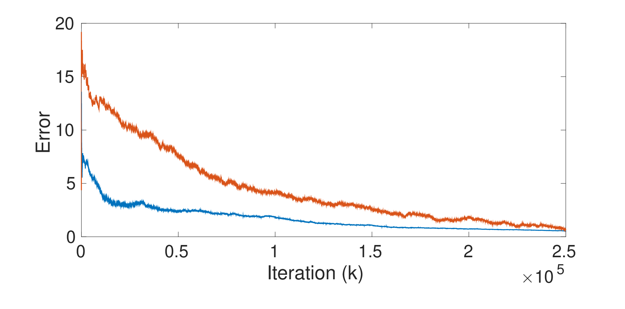
Figure 2 plots the distance to the saddle point in the primal and dual spaces when all agents are truthful. The final error values were and , indicating close convergence in each space despite the large amount of noise in the system.
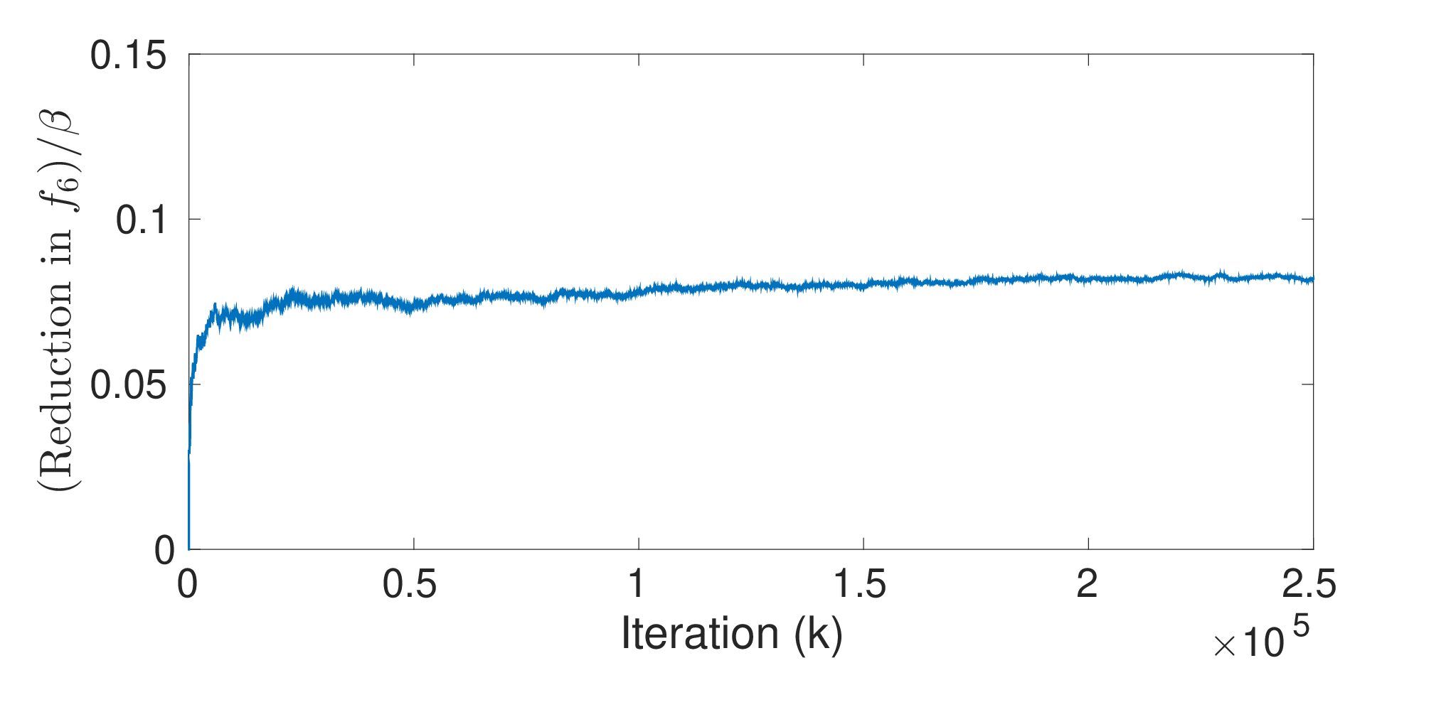
Figure 3 plots the decrease in cost agent sees in misreporting its state. This decrease is not only bounded by , but is bounded above by for all time, indicating that may be loose in some cases; this is not surprising given that uses Lipschitz constants and set diameters, which are “worst-case” in the sense that they give maximum values over all possible states. Nonetheless, the algorithm can be seen both to converge and compute a -approximate minimum, indicating that Problem 1 has been solved.
VII Conclusion
It was shown that joint differential privacy can be used in multi-agent optimization to incentivize truthful information sharing. Applications of the work presented here include any multi-agent setting in which the iterates of an optimization algorithm correspond to some physical quantity of interest. Future directions include allowing asynchronous communications in order to account for systems with communication latency and poor channel quality.
References
- [1] AB Bakushinskii and BT Polyak. Solution of variational inequalities. Doklady Akademii SSSR, 219(5):1038–1041, 1974.
- [2] Dimitri P Bertsekas, Angelia Nedic, and Asuman E Ozdaglar. Convex analysis and optimization. Athena Scientific, 2003.
- [3] S. Boyd, N. Parikh, E. Chu, B. Peleato, and J. Eckstein. Distributed optimization and statistical learning via the alternating direction method of multipliers. Found. Trends Mach. Learn., 3(1), January 2011.
- [4] S. Braynov and M. Jadliwala. Detecting malicious groups of agents. In Multi-Agent Security and Survivability, 2004 IEEE First Symposium on, pages 90–99, Aug 2004.
- [5] Jorge Cortes, Sonia Martinez, Timur Karatas, and Francesco Bullo. Coverage control for mobile sensing networks. In Robotics and Automation, 2002. Proceedings. ICRA’02. IEEE International Conference on, volume 2, pages 1327–1332. IEEE, 2002.
- [6] C. Dwork and A. Roth. The algorithmic foundations of differential privacy. Theoretical Computer Science, 9(3-4):211–407, 2013.
- [7] Cynthia Dwork, Frank McSherry, Kobbi Nissim, and Adam Smith. Calibrating noise to sensitivity in private data analysis. In Proc. of the Third Conference on Theory of Cryptography, TCC’06, pages 265–284, Berlin, Heidelberg, 2006. Springer-Verlag.
- [8] A. Fagiolini, M. Pellinacci, G. Valenti, G. Dini, and A. Bicchi. Consensus-based distributed intrusion detection for multi-robot systems. In Robotics and Automation, 2008. ICRA 2008. IEEE International Conference on, pages 120–127, May 2008.
- [9] M.T. Hale and M. Egerstedt. Cloud-enabled multi-agent optimization with constraints and differentially private states. 2016. Submitted for publication. Available at http://arxiv.org/abs/1507.04371.
- [10] S. Han, U. Topcu, and G. J. Pappas. Differentially private distributed constrained optimization. IEEE Transactions on Automatic Control, PP(99):1–1, 2016.
- [11] Shuo Han, U. Topcu, and G.J. Pappas. An approximately truthful mechanism for electric vehicle charging via joint differential privacy. In American Control Conference (ACC), 2015, July 2015.
- [12] Justin Hsu, Zhiyi Huang, Aaron Roth, and Zhiwei Steven Wu. Jointly private convex programming. In Proc. of the 27th Annual ACM-SIAM Symposium on Discrete Algorithms, SODA ’16, 2016.
- [13] M. Kearns, M. Pai, A. Roth, and J. Ullman. Mechanism design in large games: Incentives and privacy. CoRR, abs/1207.4084, 2012.
- [14] H. W. Kuhn and A. W. Tucker. Nonlinear programming. In Proc. of the 2nd Berkeley Symposium on Math. Stat. and Prob., Berkeley, Calif., 1951. University of California Press.
- [15] J. Le Ny and G.J. Pappas. Differentially private filtering. Automatic Control, IEEE Transactions on, 59(2):341–354, Feb 2014.
- [16] Frank McSherry and Kunal Talwar. Mechanism design via differential privacy. In Proceedings of the 48th Annual IEEE Symposium on Foundations of Computer Science, FOCS ’07, pages 94–103, Washington, DC, USA, 2007. IEEE Computer Society.
- [17] M.H. Nazari, Z. Costello, M.J. Feizollahi, S. Grijalva, and M. Egerstedt. Distributed frequency control of prosumer-based electric energy systems. Power Systems, IEEE Transactions on, 29(6), Nov 2014.
- [18] BT Poljak. Nonlinear programming methods in the presence of noise. Math. programming, 14(1):87–97, 1978.
- [19] Daniel E Soltero, Mac Schwager, and Daniela Rus. Decentralized path planning for coverage tasks using gradient descent adaptive control. The International Journal of Robotics Research, 2013.