Stellar oscillations - the adiabatic case

B. Mosser Address: LESIA, CNRS, Université Pierre et Marie Curie, Université Denis Diderot, Observatoire de Paris, 92195 Meudon cedex, France

Abstract

This lecture on adiabatic oscillations is intended to present the basis of asteroseismology and to serve as an introduction for other lectures of the EES 2014. It also exposes the state-of-the-art of solar-like oscillation analysis, as revealed by the space missions CoRoT and Kepler. A large part of the lecture is devoted to the interpretation of the modes with a mixed character that reveal the properties of the radiative cores of subgiants and red giants.

1 Introduction

1.1 Aim of this lecture

The favorite activity of a seismologist consists in seeking to look much below the surface of his preferred object, as everyone who prefers a deep to a superficial analysis, to get to the bottom of things, to look an issue in more depth, to delve into something, to get to the root of the matter, to seek out the underlying issue… This was the program proposed by Athanasius Kircher, a German Jesuit (1601-1680), in his model of the Earth’s interior: volcanoes were seen as outlets of the Earth’s internal fires (Fig. 1). This is the program proposed by the 2014 Évry Schatzman School: Astérosismologie et nouvelles contraintes sur les modèles stellaires / Asteroseismology and new constraints for stellar modelling.

Attendees of the EES were all supposed to have a background in physics at the Master level, including a background in hydrodynamics. Nevertheless, the first chapters are intended to smoothly introduce the physics of the stellar (or solar) oscillations. This introduction chapter presents relevant definitions and terms on which we have to agree. Chapter 2 deals with the propagation of waves, in the general case applicable to the interior of the stars, but limited to the adiabatic case. So, any energy exchanged between the wave and the star interior is here neglected and omitted; non-adiabatic oscillations are considered in the contribution to the EES 2014 by Samadi & Belkacem.

Chapter 3 shows how the adiabatic oscillation waves become modes when boundary conditions are used. It also shows the acute power of asteroseismology for probing efficiently stellar interiors.

Chapter 4 presents the wealth of information to be gained from oscillation frequencies. This information first relies on the identification of the pattern, then on the link between global¹¹ 1 Global seismic parameters are integrated quantities. They are also known as seismic indices since they present the double properties of being observable and being related to the stellar mass and radius. seismic parameters and interior structure information; the asymptotic²² 2 Here, asymptotic means, in practice, valid in the high-frequency domain. expansion helps providing both information. Then, global seismic parameters, frequency differences, or frequencies are analyzed for making the best of the seismic information.

Chapter 5 is devoted to ensemble asteroseismology: even if restricted to global seismic parameters, seismology already delivers key information on the stellar interior structure and can provide valuable information on large ensemble of stars, in a way similar to the Hertzsprung-Russell diagram (see Fig. 53).

The Appendix deals with more technical issues. Spherical harmonics are briefly presented in Section 7. Section 8 presents how asymptotic development operates. In Section 9, we see how the variational principle is used to make the best of observed oscillations spectra and address the inverse problem. Section 10 deals with rotation, and Section 11 with surface effects.

Refer to caption — Figure 1: Kircher’s model of the Earth’s internal fires, from Mundus Subterraneus. Courtesy History of Science Collections, University of Oklahoma Libraries.

1.2 Tell me how you oscillate, I will tell you who you are

A few examples may highlight the physical concept behind seismology and illustrate the title of the section, freely adapted from Miguel de Cervantes, Sainte-Beuve, Antoine de Saint-Exupéry, Marcel Pagnol, and the folk wisdom.

The railway worker who hits the axletree of a wagon listens to the produced sound; any disequilibrium or crack in the wheels will induce a specific signature. If you wish to hang out the picture of your mother-in-law on a wall covered with wall paper, a flick of the fingers will indicate which type of bit has to be used to drill the wall. Similarly, music³³ 3 Hereafter denoted as global oscillations from the stars provides us with a unique view on their interior structure, as music carries a lot of information (Bach is not Eminem, and conversely). If you listen to me, you rapidly get an idea of my skills: poor English, French accent⁴⁴ 4 Still present in the written version of the lecture…, addict to red giant seismology ;-).

1.3 Definitions, vocabulary, and tricks

1.3.1 Seismology

Greek etymology helps understanding the word seismology: “seiein” [shake] + “logos” [study]. Then, we can develop seismology in helioseismology (no Earth quakes on the Sun surface, but Sun quakes, as seen in Fig. 2), asteroseismology, dioseismology (Mosser et al., 1993; Gaulme et al., 2011, e.g.,), selenoseismology (Duennebier & Sutton, 1974; Lognonné & Mosser, 1993, e.g.,)…

Asteroseismology encompasses two notions, which are physically quite different:
- solar-like oscillations, namely stochastically excited and damped oscillations;
- stellar variability, which corresponds to thermal unstable oscillations (Fig. 3).
This lecture is focussed on solar-like oscillations; the formalism is however suited to analyze oscillations in any class of pulsating stars. Solar-like oscillations have much smaller amplitudes than intrinsically unstable oscillations. Their spectra are however directly intelligible, what is not necessarily the case for unstable pulsations. With the space missions CoRoT and Kepler (Baglin et al., 2006; Borucki et al., 2010), solar-like oscillations are observed in a large variety of low-mass stars, all along their evolution from the main sequence to the upper red and asymptotic giant branches (Michel et al., 2008; De Ridder et al., 2009; Bedding et al., 2010a; Chaplin et al., 2011), as shown in Fig. 4.

1.3.2 Waves versus modes

Waves and modes are different physical concepts. A wave is propagating; a mode is a standing wave. As such, a mode does not propagate as it is stationary. Mathematically, a phase term varying as $\omega t-{\bf k}.{\bf r}$ corresponds to a wave whereas a decoupled time and space variation as $\cos\omega t.\cos{\bf k}.{\bf r}$ corresponds to a mode. Anyway, any mode can be obtained by a sum of waves, and any wave can be obtained by a sum of modes as well.

Angular frequency ( $\omega=2\pi\nu$ ) and cyclic frequency ( $\nu=\omega/2\pi$ ) carry similar information but are used in different contexts. When studying waves, it is more convenient to use the angular frequency in order to have a compact expression of the phase of the wave, especially with an harmonic form $\exp i\omega t$ . When boundary conditions are introduced, the concept of normal modes supersedes the concept of waves. Modes are preferably characterized by their cyclic frequency.

2 Waves and propagation

This chapiter aims at presenting how waves propagate in a star. For more information, the reader can refer to Unno et al. (1989) and to Cox (1980) (Aerts et al., 2010, see also)).

2.1 Equations describing the fluid

The temporal variation of a mass element of a fluid, inside a volume $V$ surrounded by a surface $S$ , is related to the conservation of mass

{{\rm d}\over{\rm d}t}\int\!\!\!\!\!\int\!\!\!\!\!\int_{V}\rho\ {\rm d}V\ =\ -\int\!\!\!\!\!\int_{S}\rho\ {\bf v}.{\bf n}\ {\rm d}S,

(1)

where $\rho$ is the density and ${\bf v}$ is the particle velocity. The negative sign comes from the orientation of the normal vector ${\bf n}$ towards the exterior, which is opposite to the usual sign convention that counts positively what is entering the system. Using Ostrogradski’s theorem⁵⁵ 5 for any vector $\mathbf{A}$ , $\int\!\!\!\int\!\!\!\int_{V}{\bm{\nabla}}.{\bf A}\ {\rm d}V\ =\ \int\!\!\!\int_{S}{\bf A}.{\bf n}\ {\rm d}S$ , the previous equation, known as the equation of mass continuity, can be rewritten

{{\rm d}\rho\over{\rm d}t}+\rho\ {\bm{\nabla}}.{\bf v}\ =\ 0.

(2)

When rotation, viscosity, and electromagnetic forces are neglected, the equation of motion writes

{\partial{\bf v}\over\partial t}+\bigl[{\bf v}.{\bm{\nabla}}\bigr]{\bf v}\ =\ -{{\bm{\nabla}}p\over\rho}+{\bf g},

(3)

where $\bf g$ is the gravity field, which derives from the gravity potential $\psi$ and depends on the density $\rho$ :

{\bf g}\ =\ -{\bm{\nabla}}\psi\ \ \hbox{ and }\ \ \nabla^{2}\psi\ =\ 4\pi{\cal G}\rho.

(4)

The energy equation is quite a complex issue, treated in Samadi & Belkacem’s lecture. For the following, we suppose that adiabaticity is met: over a cycle, there is no energy exchanged between the wave and the fluid. This is justified by the fact that the temporal evolution of the wave is much more rapid than the characteristic time of any mechanism transferring energy as heat between the different fluid elements.

If, as in the following part, we note $\rho$ and $p$ the Eulerian perturbations associated to the oscillations (and with a subscript $\tiny 0$ for the variables at equilibrium), the energy equation is then

\left({{\rm d}\ln p\over{\rm d}\ln\rho}\right)_{\mathrm{ad}}\ \stackrel{{\scriptstyle\mathrm{def}}}{{=}}\ \ \Gamma_{1}.

(5)

It helps defining the first adiabatic exponent $\Gamma_{1}$ . As one can imagine, this relation if of prime importance for this lecture on adiabatic oscillations. There is no phase lag between the pressure perturbation and the density perturbation, contrary to the non-adiabatic case.

2.2 Linearization

2.2.1 Euler versus Lagrange

To develop the characteristics of the fluid dynamics, we have to choose a way to treat the variables. On the one side, the Eulerian (fixed-position) approach describes the physics of a fluid in terms of fields. On the other side, the Lagrangian description corresponds to the case where a fluid element is individually followed. The position of the particle varies with time. Mathematically, these different points of view are reconciled with the operator relation

{{\rm d}\over{\rm d}t}\ =\ {\partial\over\partial t}+{{\rm d}{\bf r}\over{\rm d}t}.{\nabla}\ =\ {\partial\over\partial t}+{\bf v}.{\nabla}

(6)

\delta x\ =\ x+{\bf\delta r}.\nabla x_{0},

(7)

with the following notations:

\left\{\begin{array}[]{rl}\hbox{Variable at equilibrium: }&x_{0}\\ \hbox{Eulerian perturbation: }&x\\ \hbox{Lagrangian perturbation: }&\delta x\\ \end{array}\right.

(8)

In the literature, Eulerian perturbations are often denoted with a prime, so that there is no confusion between a variable $x$ , its value at equilibrium $x_{0}$ , and its Eulerian perturbation $x^{\prime}$ . Since the next Section introduces the linearization of the wave, we prefer to lighten the equations and to avoid introducing primes.

In the following, equations are written according to the Eulerian specification of the flow field. However, in many cases it is necessary to go back to the Lagrangian form, for situations where localization matters. For instance, referring to a boundary condition requires the use of the Lagrangian approach.

2.2.2 Notations

Interior structure variables are marked with an index 0 to distinguish them from the Eulerian perturbations. So, pressure, density, velocity field, and gravity field (or gravity potential) are denoted:

\displaystyle\left\{\begin{array}[]{rccccl}\hbox{At equilibrium:}&p_{0},&\rho_{0},&{\bf 0},&{\bf g_{0}}&(\hbox{or\ }\psi_{0})\\ \hbox{Eulerian perturbation:}&p,&\rho,&{\bf v},&{\bf g}&(\hbox{or\ }\psi)\\ \end{array}\right.

Perturbations, if small, can be treated at first order. This provides a linearized approach, which is evidently much simpler than the complete approach since non-linearity is discarded. So, as soon as the linear approach is chosen, some tricky problems cannot be considered any more, as those concerning the amplitude of the waves. In other words, the eigenvalue problem can be solved to the first order, but the absolute amplitude of eigenfunctions will remain undetermined.

We also consider that the equilibrium structure obeys the hydrostatic equilibrium. This relies on the assumption of stationarity and of absence of any movement at equilibrium. For any interior structure parameter $x_{0}$ , this implies

{\partial x_{0}\over\partial t}\ =\ 0.

(12)

Accordingly velocity field is zero. This also means that we consider non-rotating stars. Including rotation would require either a specific study or a perturbation treatment. Rotation is briefly presented, as a perturbation only, in Appendix 10. Rapidly rotating stars requires a specific non-pertubative study (e.g., Reese et al., 2009; Ouazzani & Goupil, 2012, and references therein).

We can thus rewrite the equations describing the fluid (Section 2.1). With the preceeding hypothesis, the advection term ${\bf v}.\nabla{\bf v}$ in the equation of motion (Eq. 3) is a second-order term and can be neglected. So, the equation of motion writes

(\rho_{0}+\rho){\partial{\bf v}\over\partial t}\ =\ -{\bm{\nabla}}(p_{0}+p)-(\rho_{0}+\rho){\bm{\nabla}}(\psi_{0}+\psi).

(13)

To go further, we use the hydrostatic equilibrium

{\bm{\nabla}}p_{0}\ =\ -\rho_{0}\ {\bm{\nabla}}\psi_{0},

(14)

so that, to first order, one gets

{\partial{\bf v}\over\partial t}\ =\ -{1\over\rho_{0}}\ {\bm{\nabla}}p-{{\bm{\nabla}}\psi_{0}\over\rho_{0}}\ \rho-{\bm{\nabla}}\ \psi.

(15)

On the right-hand term, it is easy to recognize three contributions to the restoring force: pressure gradient; buoyancy; perturbation of the gravitational potential.

To first order, the mass conservation (Eq. 2), rewritten as

{\partial(\rho_{0}+\rho)\over\partial t}+{\bm{\nabla}}.((\rho_{0}+\rho){\bf v})\ =\ 0,

(16)

becomes

{\partial\rho\over\partial t}+{\bm{\nabla}}.(\rho_{0}{\bf v})\ =\ 0.

(17)

The previous form of the Poisson equation (4) being linear, it simply rewrites

\nabla^{2}\psi\ =\ 4\pi{\cal G}\rho.

(18)

Eq. (5) that expresses the adiabatic propagation becomes

{{\rm d}p\over{\rm d}t}\ =\ \Gamma_{1}{p_{0}\over\rho_{0}}\ {{\rm d}\rho\over{\rm d}t}.

(19)

This is a Lagrangian form, corresponding to the Eulerian form

{\partial p\over\partial t}+{\bf v}.{\bm{\nabla}}p_{0}\ =\ \Gamma_{1}{p_{0}\over\rho_{0}}\ \left({\partial\rho\over\partial t}+{\bf v}.{\bm{\nabla}}\rho_{0}\right).

(20)

Combinations with the hydrostatic equilibrium and the mass conservation then provide

{\partial p\over\partial t}\ =\ -\Gamma_{1}p_{0}\ {\bm{\nabla}}.{\bf v}-\rho_{0}\ {\bf g_{0}}.{\bf v}.

(21)

2.3 Sound waves

Here, we consider a highly simplified case for introducing useful concepts, methods and parameters. We consider the case of a plane-parallel atmosphere and no gravity gradient. Moreover, all gradients in the interior structure are neglected, so that all scale heights are much larger than the wavelength $\lambda$ . The scale height $H_{\mathrm{X}}$ of any equilibrium variable $X$ (such as temperature, pressure, density, sound speed, adiabatic gradient…) is defined by $H_{\mathrm{X}}=(-{\rm d}\ln X/{\rm d}r)^{-1}$ .

Pressure and density inside the Sun are plotted in Fig. 5; their scale heights are given in Fig. 6. This shows that the assumptions as presented are not adapted to study solar pressure waves; this paragraph intends to present a case study and not a realistic description of sound waves inside the Sun. We also suppose the Cowling approximation (Cowling, 1941): the Eulerian perturbation of the gravitational potential is neglected in the equation of motion (Eq. 15).

We introduce the harmonic description

{\partial\over\partial t}=i\omega,

(22)

taking into account the temporal variation of all perturbed terms varying as $\exp i\omega t$ . So, from the adiabatic relation (Eq. 19)

i\omega p\ =\ \Gamma_{1}{p_{0}\over\rho_{0}}i\omega\rho,

(23)

we get

p\ =\ \Gamma_{1}\displaystyle{p_{0}\over\rho_{0}}\rho\ =\ c_{0}^{2}\rho.

(24)

The sound speed profile (Fig. 7) is defined by

c_{0}^{2}\ \ \stackrel{{\scriptstyle\mathrm{def}}}{{=}}\ \ \left({\partial p\over\partial\rho}\right)_{\mathrm{S}}\ \ \stackrel{{\scriptstyle\mathrm{def}}}{{=}}\ \ \Gamma_{1}\ \displaystyle{p_{0}\over\rho_{0}}.

(25)

Note that this definition is independent on the approximations used in the simplified case.

In an isothermal atmosphere, at temperature $T_{0}$ , where the classical non-degenerate perfect gas law is relevant, Eq. (25) reduces to

c_{0}^{2}\ =\ \displaystyle{\Gamma_{1}k_{\mathrm{B}}T_{0}\over\mu},

(26)

where $\mu$ is the mean particle mass, so that the temperature and sound-speed profiles are closely linked (Fig. 7).

According to the set of hypothesis previously defined, perturbations are described by:

\displaystyle\left\{\begin{array}[]{rcl}i\omega\ \rho_{0}{\bf v}&=&-{\bm{\nabla}}p\\ i\omega\ \rho+\rho_{0}\ {\bm{\nabla}}.{\bf v}&=&0\\ p&=&c_{0}^{2}\ \rho\\ \end{array}\right.

In the equation of motion, the restoring force reduces to the pressure gradient owing to hypothesis on the scale heights. The expressions of $p$ and ${\bf v}$ can be eliminated for obtaining an equation for $\rho$

-\omega^{2}\rho=-i\omega\ \rho_{0}\ {\bm{\nabla}}.{\bf v}=+{\bm{\nabla}}.{\bm{\nabla}}p=\Delta\ p=c_{0}^{2}\ \Delta\rho.

(31)

Under the hypothesis that the wave is a plane wave, the phase of the wave varies as

\exp i\ \bigl[wt-{\bf k}.{\bf r}\bigr]

so that $\mathbf{\nabla}\equiv-i\mathbf{k}$ and $\Delta\equiv-k^{2}$ . Therefore, we obtain the dispersion relation

\omega^{2}\ =\ k^{2}c_{0}^{2}.

(32)

Owing to all simplifications already made, this equation is in fact not dispersive: the phase velocity $\omega/k$ and group velocity ${\rm d}\omega/{\rm d}k$ are the same for all wavelengths.

2.4 Gravity waves

The main restoring force of a gravity wave is not due to pressure gradient but to buoyancy: a particle moved away from its equilibrium position has to find it again due to the disequilibrium in density. This happens when the motion is slow enough for ensuring that the pressure equilibrium is achieved. Indeed, gravity waves have a cyclic frequency smaller than the dynamic frequency $2\pi/t_{\mathrm{dyn}}$ associated to the dynamic time. However, the motion is rapid enough for ensuring that the movement is adiabatic. As a result, the density of the perturbation differs from the local density in the fluid. Necessarily, gravity waves cannot exist in convective regions since the Schwarzschild criterion expresses that buoyancy cannot provide a restoring force in a convective region since it is the disturbing force that moves convective cells.

As for the sound waves, we address a simplified case of gravity waves that can be expressed in terms of plane waves. The vertical and horizontal components of the wave vector $\bf k$ are noted $k_{\mathrm{v}}$ and $k_{\mathrm{h}}$ , respectively. For sake of simplicity, we do not consider the vector behavior of the horizontal component of $\bf k$ . As for sound waves, we apply the Cowling approximation (Cowling, 1941): in the equation of motion (Eq. 15), the Eulerian perturbation of the gravitational potential is neglected.

2.4.1 The dispersion relation

The motion and mass equations (Eq. 15 and 17) express then

\displaystyle\left\{\begin{array}[]{rcl}i\omega\ \rho_{0}v_{\mathrm{h}}&=&ik_{\mathrm{h}}\ p\\ i\omega\ \rho_{0}v_{\mathrm{v}}&=&ik_{\mathrm{v}}\ p-g_{0}\ \rho\\ i\omega\ \rho&=&\rho_{0}\left(ik_{\mathrm{h}}\ v_{\mathrm{h}}+ik_{\mathrm{v}}\ v_{\mathrm{v}}\right)\\ \end{array}\right.

Hence, the horizontal component of the velocity is

v_{\mathrm{h}}\ =\ {k_{\mathrm{h}}\over\rho_{0}\omega}\ p.

(37)

Using the mass equation, we have

v_{\mathrm{h}}={\omega\over k_{\mathrm{h}}}\ {\rho\over\rho_{0}}-{k_{\mathrm{v}}\over k_{\mathrm{h}}}v_{\mathrm{v}}.

(38)

This result is used in the equation of the vertical movement

i\omega\ \rho_{0}v_{\mathrm{v}}=\left(ik_{\mathrm{v}}\ {\omega^{2}\over k_{\mathrm{h}}^{2}}-g_{0}\right)\ \rho-\rho_{0}i\omega\ {k_{\mathrm{v}}^{2}\over k_{\mathrm{h}}^{2}}\ v_{\mathrm{v}}.

(39)

The right-hand term of this expression is composed of terms in $\rho$ and $v_{\mathrm{v}}$ . Since we only deal with long-period waves, the coefficient proportional to $\omega^{2}$ is negligible compared to the other terms, so that:

i\omega\ \rho_{0}\ \left(1+{k_{\mathrm{v}}^{2}\over k_{\mathrm{h}}^{2}}\right)\ v_{\mathrm{v}}\ =\ -g_{0}\ \rho.

(40)

This equation shows that the vertical motion is mainly due to the buoyancy term. The inertia of the displacement increases for low values of the horizontal wavenumber. The coupling between the vertical and horizontal motions results from the conservation of the mass.

Finally, we have to introduce the adiabatic evolution of the system (Eq. 20):

i\omega\ p+v_{\mathrm{v}}{{\rm d}p_{0}\over{\rm d}r}\ =\ \Gamma_{1}{p_{0}\over\rho_{0}}\ \left(i\omega\ \rho+v_{\mathrm{v}}{{\rm d}\rho_{0}\over{\rm d}r}\right).

(41)

In the left-hand term of this equation, the contribution of $p$ can be neglected with respect to the contribution of $v_{\mathrm{v}}$ since it is proportional to $\omega^{2}$ (Eq. 38). So, adiabaticity gives

v_{\mathrm{v}}\left({{\rm d}p_{0}\over{\rm d}r}-\Gamma_{1}{p_{0}\over\rho_{0}}\ {{\rm d}\rho_{0}\over{\rm d}r}\right)\ =\ i\omega\ \Gamma_{1}{p_{0}\over\rho_{0}}\ \rho.

(42)

Hence, with the introduction of the density scale height,

v_{\mathrm{v}}\left(1-\displaystyle{1\over\Gamma_{1}}\displaystyle{{\rm d}\log p_{0}\over{\rm d}\log\rho_{0}}\right)\ {\rho_{0}\over H_{\rho}}\ =\ i\omega\ \rho.

(43)

Combination with Eq. (40) provides

\omega^{2}\rho_{0}\ \left(1+{k_{\mathrm{v}}^{2}\over k_{\mathrm{h}}^{2}}\right)\ v_{\mathrm{v}}\ =\ \left(1-\displaystyle{1\over\Gamma_{1}}\displaystyle{{\rm d}\log p_{0}\over{\rm d}\log\rho_{0}}\right)\ {g_{0}\rho_{0}\over H_{\rho}}\ v_{\mathrm{v}}

(44)

This gives the dispersion relation

\omega^{2}\ \left(1+{k_{\mathrm{v}}^{2}\over k_{\mathrm{h}}^{2}}\right)\ =\ {g_{0}\over H_{\rho}}\ \left(1-\displaystyle{1\over\Gamma_{1}}\displaystyle{{\rm d}\log p_{0}\over{\rm d}\log\rho_{0}}\right)\ =\ N_{\mathrm{BV}}^{2}.

(45)

So, with the introduction of the Brunt-Väisälä frequency discussed in the next paragraph, the relation between the horizontal and vertical components of the wavevector is

k_{\mathrm{v}}^{2}\ =\ \left({N_{\mathrm{BV}}^{2}\over\omega^{2}}-1\right)k_{\mathrm{h}}^{2}.

(46)

2.4.2 Brunt-Väisälä frequency

The dispersion relation (Eq. 45) makes use of the Brunt-Väisälä frequency $N_{\mathrm{BV}}$ . This frequency helps comparing the real gradient $\Gamma$ in the fluid to the adiabatic gradient $\Gamma_{1}$ :

N_{\mathrm{BV}}^{2}\ \ \stackrel{{\scriptstyle\mathrm{def}}}{{=}}\ \ {g_{0}\over H_{\rho}}\ \left(1-\displaystyle{\left.\displaystyle{{\rm d}\log p\over{\rm d}\log\rho}\right|_{\mathrm{fluid}}\over\left.\displaystyle{{\rm d}\log p\over{\rm d}\log\rho}\right|_{\mathrm{adiab}}}\right)={g_{0}\over H_{\rho}}\ \left(1-{\Gamma\over\Gamma_{1}}\right).

(47)

According to the definition, $N_{\mathrm{BV}}=0$ in a convective region (Fig. 8, 9). In fact, the small overadiabaticity necessary to evacuate the stellar energy makes that $N_{\mathrm{BV}}^{2}<0$ . This confirms that gravity waves cannot propagate in a convective region. In the Sun, gravity waves are trapped in the inner radiative region. Their detection is highly difficult due to their evanescent evolution in the convective envelope (Belkacem et al., 2009; Appourchaux et al., 2010).

Different forms for expressing $N_{\mathrm{BV}}$ can be found in the literature. Eq. (47) can write

N_{\mathrm{BV}}^{2}\ =\ g_{0}\ \left({1\over\Gamma_{1}p_{0}}{{\rm d}p_{0}\over{\rm d}r}-{1\over\rho_{0}}{{\rm d}\rho_{0}\over{\rm d}r}\right).

(48)

Under the assumption of the ideal gas law for a fully ionized gas, and taking the composition gradient into account, the expression becomes (Unno et al., 1989, Section 13.4 of )

N_{\mathrm{BV}}^{2}\ =\ {g_{0}^{2}\rho_{0}\over p_{0}}\ \left(\nabla_{\mathrm{ad}}-\nabla+\nabla_{\mu}\right),

(49)

with

\nabla_{\mathrm{ad}}=\left({\partial\ln T_{0}\over\partial\ln p_{0}}\right)_{\mathrm{ad}},\ \nabla={{\rm d}\ln T_{0}\over{\rm d}\ln p_{0}},\hbox{ and }\nabla_{\mu}={{\rm d}\ln\mu\over{\rm d}\ln p_{0}}.

(50)

In a plane-parallel atmosphere with a uniform gravity field, it simplifies into.

N_{\mathrm{BV}}^{2}\ =\ g_{0}\ \left({1\over H_{\rho}}-{g_{0}\over c_{0}^{2}}\right).

(51)

The contribution of the gravity term in the Brunt-Väisälä frequency yields the increase of $N_{\mathrm{BV}}$ in the stellar interior when the star evolves, as a result of the contracting core (Fig. 10).

According to Eq. (45), the frequency of a gravity wave is necessarily below the Brunt-Väisälä frequency $N_{\mathrm{BV}}$ since one has

{k_{\mathrm{h}}\over k}={\omega\over N_{\mathrm{BV}}}.

(52)

In the low-frequency regime, with $\omega\ll N_{\mathrm{BV}}$ , we have $k_{\mathrm{h}}\ll kv$ . Otherwise when $\omega$ is close to $N_{\mathrm{BV}}$ , we have have $k_{\mathrm{h}}\approx k$ .

2.5 Surface gravity waves

We may use the previous equations to derive the dispersion equation at the surface of a fluid object, or at the boundary between two immiscible fluids. We also suppose the plane-parallel case, and the fluid to be incompressible.

From incompressibility, the mass equation (Eq. 17) gives

{\bm{\nabla}}.{\bf v}\ =\ 0.

(53)

If the gradient and the perturbation of the gravitational potential are neglected, the equation of motion is

\rho_{0}{\partial{\bf v}\over\partial t}\ =-{\bm{\nabla}}p.

(54)

The perturbed pressure then obeys to

\Delta\ p\ =\ 0.

(55)

We aim to search for a periodic solution, moving parallel to the surface or to the interface. With $z$ the variable of the axis perpendicular to the surface and $x$ along this surface, we have

p\ =\ P(z)\exp i(\omega t-kx).

(56)

Using Eq. (56) in Eq. (55) gives

{{\rm d}^{2}P\over{\rm d}z^{2}}-k^{2}P\ =\ 0.

(57)

Hence $P(z)$ writes:

P(z)\ =\ P_{-}\exp(-kz)+P_{+}\exp(+kz).

(58)

The diverging solution must be excluded if the width of the layer is large. At the surface, pressure equilibrium implies that the Lagrangian perturbation is null. This is typically a case where, despite the solution found with Eulerian variables, it is necessary to use the Lagrangian term to express the properties of a boundary:

{{\rm d}p\over{\rm d}t}\ =\ {\partial p\over\partial t}+{\bf v}.{\bm{\nabla}}{p_{0}}\ =\ {\partial p\over\partial t}+\rho_{0}{\bf v}.{\bf g_{0}}\ =\ 0.

(59)

Without information on the surface (presumably it just has small variations around $z=0$ ), we can get the dispersion equation when combining Eq. (59) with the equation of vertical motion (Eq. 54)

\displaystyle\left\{\begin{array}[]{rll}\displaystyle{\partial p\over\partial t}&+\rho_{0}g_{0}\ v_{z}&=0,\\ \rho_{0}\displaystyle{\partial v_{z}\over\partial t}&+\displaystyle{\partial p\over\partial z}&=0.\\ \end{array}\right.

This gives

\displaystyle{\partial^{2}p\over\partial t^{2}}\ =\ g_{0}\displaystyle{\partial p\over\partial z},

(63)

hence the dispersion equation

\omega^{2}=\ g_{0}k.

(64)

The equation of the free surface, with no Lagrangian perturbation, is then

\delta p=p+{\bm{\xi}}.{\bm{\nabla}}p_{0}=0,

(65)

where ${\bm{\xi}}$ is the wave displacement. Hence

\xi_{\mathrm{v}}={1\over\rho_{0}g_{0}}\ p.

(66)

In such a case, the group velocity ${\rm d}\omega/{\rm d}k$ is half the phase velocity $\omega/k$ . This can be easily seen when throwing a small stone in a pond. Such waves resembles the fundamental waves, at the limit between pressure and gravity waves (Section 4.7).

2.6 Differences between pressure waves and gravity waves

This paragraph aims at emphasizing the difference between pressure and gravity waves. It also shows the relevance of the Cowling approximation. Heavy assumptions are used for hand-made physics based on Eqs. (15) and (18).

\displaystyle\left\{\begin{array}[]{rrll}\hbox{Motion equation:}&\rho_{0}\ \displaystyle{\partial{\bf v}\over\partial t}&=&-\nabla p+\displaystyle{\nabla p_{0}\over\rho_{0}}\ \rho-\rho_{0}\ \nabla\ \psi\\ \hbox{Poisson equation:}&\nabla^{2}\psi&=&4\pi{\cal G}\rho\\ \end{array}\right.

2.6.1 Pressure waves

For high-frequency waves, the operation of partial derivative with respect to time, $\partial/\partial t$ , provides much bigger terms than the gradient operator. Adiabatic evolution implies, as a consequence of the definition of $\Gamma_{1}$ (Eq. 25):

p\ =\ \Gamma_{1}{p_{0}\over\rho_{0}}\ \rho\ =\ c_{0}^{2}\ \rho.

(70)

In the inner regions, sound speed and gravity verify

c_{0}^{2}\propto{\cal G}M/R\propto g_{0}\ R.

(71)

For a crude estimate of the restoring forces, one can use the following approximations for the gradients

\displaystyle\left\{\begin{array}[]{rlcr}\hbox{equilibrium:}&\nabla X_{0}&\simeq&X_{0}/R,\\ \hbox{perturbation:}&\nabla X&\simeq&nX/R,\\ \end{array}\right.

where $n$ is the number of wavelengths along the stellar radius.

From the Poisson equation, one derives $\nabla^{2}\psi\simeq n^{2}\,\psi/R^{2}$ , hence $\psi\simeq 4\pi{\cal G}R^{2}\rho/n^{2}$ . Accordingly, the three components of the restoring force can be estimated:

\displaystyle\left\{\begin{array}[]{rrllllll}\hbox{pressure:}&\displaystyle{\nabla p}&\simeq n\ \displaystyle{p\over R}&\simeq n\ \displaystyle{c_{0}^{2}\over R}\ \rho&\propto&n&g_{0}\ \vrule height=10.0pt,depth=5.0pt,width=0.0pt\rho,\\ \hbox{buoyancy:}&\displaystyle{\nabla p_{0}\over\rho_{0}}\ \rho&&&\propto&&g_{0}\ \rho,\\ \hbox{potential:}&\rho_{0}\ \nabla\ \psi&\simeq 4\pi{\cal G}R\rho_{0}\displaystyle{\rho\over n}&\propto\displaystyle{1\over n}\displaystyle{c_{0}^{2}\over R}\ \rho&\propto&\displaystyle{1\over n}&g_{0}\ \rho.\\ \end{array}\right.

The pressure term evidently dominates the restoring force when the number $n$ is large: this is a pressure wave. Furthermore, the perturbation of the gravitational potential is the smallest term. This justifies the Cowling approximation (see paragraph 3.2.5).

2.6.2 Gravity waves

Gravity waves evolves slowly with time. In that case, spatial gradient terms are dominating the terms obtained from the operator $\partial/\partial t$ , so that Eq. (2.6) gives, when we assume that the perturbation of the gravitational potential can be neglected:

\displaystyle\begin{array}[]{ccclc}&\nabla p&\simeq&\displaystyle{\nabla p_{0}\over\rho_{0}}&\rho,\\ n&\displaystyle{p\over R}&\simeq&\displaystyle{p_{0}\over R\rho_{0}}&\rho,\\ n&p&\simeq&c_{0}^{2}&\rho.\\ \end{array}

This means that the pressure gradient and the buoyancy term are equilibrated. Compared to a pressure wave for which the pressure and density perturbations are linked with $p_{\mathrm{p}}=c_{0}^{2}\rho$ , here we have $p_{\mathrm{g}}=c_{0}^{2}\rho/n$ . Hence, the pressure perturbation $p_{\mathrm{g}}$ verifies $p_{\mathrm{g}}\ll c_{0}^{2}\rho$ . This is a gravity wave.

3 Global oscillations

As seen in the previous chapter, four variables are used for describing the oscillations in a non-rotating object: pressure $p$ , density $\rho$ , velocity field ${\bf v}$ , and gravity field $\bf g$ (or gravitational potential $\psi$ ). These terms, defined as small perturbations, are bound with a set of four equations: equation of motion, continuity equation, Poisson equation, and energy equation.

A few hypotheses for studying global oscillations in a star are implicitly present: taking small perturbations into account yields linear equations; rotation being neglected, spherical symmetry is used. Different treatments can be made, depending on the set of hypotheses. In this chapter, we do not intend to redo all calculations from the physical equations to the dispersion equation. These calculations are available in many references (Aerts et al., 2010, e.g.,). We just point out a few important steps in the understanding of the physics. The aim is to obtain a propagation diagram (Section 3.3). A solution of the eigenvalue problem, the asymptotic expansion, is presented in the next chapter.

The choice of the hypothesis used for simplifying and reducing the size the differential equation system plays a significant role, as one can imagine. Among the main hypothesis (and apart from the non-rotating spherical case already mentioned), we can find the following cases:
- Plane-parallel atmosphere, corresponding in practice to neglect the spherical case; this can be useful for phenomena in the upper stellar envelope but cannot fit a real case of a spherically symmetric star;
- Cowling approximation: the perturbation of the gravitational field plays a negligible role in the equations. With the Cowling approximation, this term is omitted; this interestingly simplifies the computation (Cowling, 1941);
- Ray-tracing: the properties of the eigenfunctions are omitted when the dispersion equation is obtained, and the wave is described by the properties of the wave vector only.

The most fertile approach is the JWKB approximation, used in Section 4 for delivering an asymptotic solution of the eigenfrequency pattern. Here, we use it first in a very simple manner, following Gough (2007) who presents ‘an elementary introduction to the JWKB approximation’: an adequate change of variable helps simplifying the dispersion equation.

3.1 Simplified case

A simple case can help catching most of the physics of seismic waves. Therefore, we neglect the spherical symmetry, consider propagation in a plane-parallel atmosphere, and use the Cowling approximation.

Variables are:

\displaystyle\left\{\begin{array}[]{rcccc}\hbox{At equilibrium:}&p_{0},&\rho_{0},&{\bf v}_{0}={\bf 0},&{\bf g_{0}}=g_{0}\,{\bf u}_{\mathrm{r}}\\ \hbox{Eulerian perturbation:}&p,&\rho,&{\bf v},&{\bf 0}\hbox{ (Cowling approx.)}\\ \end{array}\right.

As a consequence of the simplification, only three equations are needed:

\displaystyle\left\{\begin{array}[]{rcccccl}\rho_{0}\displaystyle{\partial{\bf v}\over\partial t}&=&-&{\bm{\nabla}}p&+&{\bf g_{0}}\ \rho\hfill&\quad\hbox{Motion}\\ \displaystyle{\partial\rho\over\partial t}&=&-&{\bm{\nabla}}.(\rho_{0}{\bf v})&&\hfill\hfil&\quad\hbox{Continuity}\\ \displaystyle{\partial p\over\partial t}&=&-&\Gamma_{1}p_{0}{\bm{\nabla}}.{\bf v}&-&\rho_{0}\ {\bf g_{0}}.{\bf v}\hfill&\quad\hbox{Adiabaticity}\\ \end{array}\right.

3.1.1 Change of variables

With a dedicated change of variables (again, reading Gough (2007) is useful to understand how it works), we can describe the propagation in a form as close as possible to a plane wave. We use

\displaystyle\left\{\begin{array}[]{rcl}\eta&=&v\sqrt{\displaystyle{p_{0}\over c}},\\ {\rm d}\tau&=&\displaystyle{{\rm d}r\over c}.\\ \end{array}\right.,

where we have omitted the subscript 0 for the sound speed $c$ since there is no ambiguity. If we further assume that the adiabatic exponent $\Gamma_{1}$ is almost uniform, we get from Eq. (3.1.1) that (Mosser, 1995, e.g.,)

\eta^{2}\propto\rho_{0}\ c\ v^{2},

(93)

which means that $\eta^{2}$ varies as the kinetic energy flux. The variable $\tau$ is the acoustic radius (which is a time and not a radius). Its use helps counterbalancing the rapid variation of the sound speed.

The resolution of the set of differential equations (Eq. 3.1), in the simplified considered case and with the ad hoc change of variables, implies that the new function $\eta(\tau)$ follows the differential equation (Roxburgh & Vorontsov, 1994; Mosser, 1995, e.g.,)

{\partial^{2}\eta\over\partial\tau^{2}}+(\omega^{2}-\omega_{\mathrm{c}}^{2})\ \eta=0,

(94)

where we have introduced the harmonic time dependence $\partial/\partial t\equiv i\omega$ and the cutoff frequency $\omega_{\mathrm{c}}$ . Due to the change of variable, the expression of $\omega_{\mathrm{c}}$ derived from Eq. (94) is more complex than the original term found Lamb (1908), but is in fact very close to it. Here, we only introduce the leading term:

\omega_{\mathrm{c}}\ =\ {c\over 2H_{\rho}},

(95)

which corresponds to the term found by Lamb (1908). This frequency is small everywhere except near the surface (Fig. 11). In a convective region, the cutoff frequency $\omega_{\mathrm{c}}$ defined Eq. (95) can also be written

\omega_{\mathrm{c}}\ =\ {g\over 2c},

(96)

as is clear from the expression of sound-speed (Eq. 26) and density scale height ( $H_{\rho}=\Gamma_{1}\,H_{\mathrm{p}}=\Gamma_{1}k_{\mathrm{B}}T/\mu g=c^{2}/g$ ).

3.1.2 Dispersion equation

From Eq. (94), we can deduce the dispersion equation

\omega^{2}=\kappa^{2}+\omega_{\mathrm{c}}^{2},

(97)

if we assume a plane-wave form for $\eta(\tau)$ with an $\exp i\kappa\tau$ dependence. Note that, with the acoustic variable $\tau$ , $\kappa$ behaves as a radial wavevector but is homogeneous to an angular frequency. As shown in Fig. 11, $\omega_{\mathrm{c}}$ has small values everywhere except near the surface, so that the dispersion equation reduces to $\omega=\kappa$ . The wave behaves as a plane wave; the modulus of the kinetic energy flux $\eta$ is supposed to be nearly uniform. This is largely verified (e.g., Fig. 12, 13).

With this dispersion equation (Eq. 97), we derive the reflection of the waves with a frequency lower than the maximum frequency reached in the upper stellar atmosphere. We also retrieve the propagation of pressure waves, when $\omega_{\mathrm{c}}$ can be neglected in most regions of the stars. In fact, the expression of $\omega_{\mathrm{c}}$ is close to the expression of $N_{\mathrm{BV}}$ ⁶⁶ 6 In an isothermal atmosphere, $\omega_{\mathrm{c}}$ and $N_{\mathrm{BV}}$ have similar variation in $\mu g^{2}/k_{\mathrm{B}}T$ ,as derived from Eqs. (51) and (95)., so that gravity waves can be also derived from this expression.

From the study of the simplified case, we retain that the acoustic radius is better adapted than the radius for describing a pressure wave. Moreover, a change of variable is able to provide new variables showing reduced amplitude gradient (Fig. 12).

3.2 Differential equations

In this section, we examine the main steps for achieving a solution in the general case. The methodology for entering more complex solutions based on less strong hypotheses than those in the previous simple case is in fact basically the same: an appropriate change of variables, as done in Eq. (3.1.1), provides a new system of differential equations derived from Eq. (3.1). This system has then to be organized in a convenient way for a numerical resolution. Boundary conditions are used to solve the eigenvalue problem.

3.2.1 Chosen set of variables

The equations explaining the propagation of the waves are expressed with the following variables:

\displaystyle\left\{\begin{array}[]{rll}\hbox{vertical displacement:}&\xi_{\mathrm{r}}&\left(\hbox{so that }v_{\mathrm{r}}=\displaystyle{{\rm d}\xi_{\mathrm{r}}\over{\rm d}t}\right)\\ \hbox{pressure:}&p\\ \hbox{gravitational potential:}&\psi\\ \end{array}\right.

The time dependence, for all terms, is harmonically expressed by $\exp i\omega t$ . Similarly, the angular dependence is expressed by the spherical harmonics $Y_{\ell}^{m}$ (Appendix 7). Strictly speaking, the notations should change, in order to take this factorization into account. For simplicity, we keep it the same, but have in mind that we should move to notations $x\to\tilde{x}$ such that

x(\mathbf{r},t)\ \equiv\ \tilde{x}(r)\ Y_{\ell}^{m}(\theta,\varphi)\ \exp i\omega t.

(102)

So, slowly but surely we leave the real space for the Fourier space; the angles $\theta$ and $\phi$ , and the time $t$ are superseded with the quantum numbers $\ell$ and $m$ , and the frequency $\omega$ , respectively. As a consequence of Eq. (102), radial partial derivatives are replaced by simple derivatives in the following equations, since $\partial x/\partial r={\rm d}\tilde{x}/{\rm d}r$ .

3.2.2 Density and horizontal displacement

Compared to the set of variables used for describing the fluid (Section 2.1), with now the velocity $\bm{v}$ replaced by the displacement $\bm{\xi}$ , we have left the density and the horizontal component of the displacement in the new set of variables (Eq. 3.2.1).

It is worthwhile to express the Eulerian density perturbation as a function of the pressure perturbation and the radial displacement (Eq. 6) in order to emphasize the difference between pressure and gravity waves. From the Lagrangian form of the adiabatic propagation (Eq. 20) and from the definition of the sound speed profile (Eq. 25), we have

\rho={p\over c^{2}}+\rho_{0}\ \left({1\over c^{2}}{\bm{\nabla}}p_{0}-{\bm{\nabla}}\rho_{0}\right)\ {\bm{\xi}}.

(103)

Due the absence of horizontal gradient of structure parameters in the spherical symmetry, this simplifies into

\rho={p\over c^{2}}-\rho_{0}\ \left({1\over\Gamma_{1}H_{\mathrm{p}}}-{1\over H_{\rho}}\right)\ \xi_{\mathrm{r}}.

(104)

If we introduce the Brunt-Väisälä frequency, we get

\rho={p\over c^{2}}+{\rho_{0}\,N_{\mathrm{BV}}^{2}\over g_{0}}\ \xi_{\mathrm{r}}.

(105)

This demonstrates that the Eulerian density perturbation is always related to the Eulerian pressure perturbation and to the radial displacement. The importance of this latter term increases with increasing $N_{\mathrm{BV}}$ values, and decreases with increasing $c$ values.

Similarly, the horizontal displacement can express as a function of the pressure perturbation and the gradient of the potential (Aerts et al., 2010, e.g., section 3.3 of). This derives from the horizontal component of the equation of motion. From Eq. (15) and from the fact that interior structure parameters have no horizontal variation, one gets

\omega^{2}\,\xi_{\mathrm{h}}=\nabla_{\mathrm{h}}\left({p\over\rho_{0}}+\psi\right).

(106)

The horizontal gradient and the vectorial dependence of the horizontal displacement (Eq. 247) match, so that

\xi_{\mathrm{h}}={1\over r\omega^{2}}\ \left({p\over\rho_{0}}+\psi\right).

(107)

3.2.3 System of differential equations

We go back to the equations with the three selected variables. They obey the set of differential equations:

\displaystyle\scriptsize{\left\{\begin{array}[]{rrrr}\displaystyle{{\rm d}\xi_{\mathrm{r}}\over{\rm d}r}=&\left(\displaystyle{1\over\Gamma_{1}\,H_{\mathrm{p}}}-\displaystyle{{2\over r}}\right)\ \xi_{\mathrm{r}}&+\displaystyle{1\over\rho_{0}c^{2}}\left(\displaystyle{{S_{\ell}^{2}\over\omega^{2}}-1}\right)\ p&+\displaystyle{\ell(\ell+1)\over\omega^{2}r^{2}}\ \psi\\ \displaystyle{{\rm d}p\over{\rm d}r}=&\rho_{0}(\omega^{2}-N_{\mathrm{BV}}^{2})\ \xi_{\mathrm{r}}&-\displaystyle{1\over\Gamma_{1}\,H_{\mathrm{p}}}\ p&-\rho_{0}\ \displaystyle{{\rm d}\psi\over{\rm d}r}\\ \displaystyle{1\over r^{2}}\displaystyle{{\rm d}\over{\rm d}r}\left(r^{2}\displaystyle{{\rm d}\psi\over{\rm d}r}\right)=&\displaystyle{4\pi{\cal G}\rho_{0}\over g_{0}}N_{\mathrm{BV}}^{2}\ \xi_{\mathrm{r}}&+\displaystyle{4\pi{\cal G}\over c^{2}}\ p&+\displaystyle{\ell(\ell+1)\over r^{2}}\ \psi\\ \end{array}\right.}

Where does this come from? The aim of this lecture is not to redo calculations that are published in many places, e.g., section 14.1 of Unno et al. (1989) or section 3.3 of Aerts et al. (2010), but to help understanding how things work:
- we have here an apparent set of three differential equations for three variables; in fact, due to the double derivative of $\psi$ , this is a fourth-order system of differential equations with the four (dependent) variables $\xi_{\mathrm{r}}$ , $p$ , $\psi$ and ${\rm d}\psi/{\rm d}r$ ;
- the frequency $\omega$ has replaced all time derivatives;
- the terms $1/r$ and $1/r^{2}$ were introduced by the operators divergence ( $\mathbf{\nabla}$ ) et Laplace operator ( $\nabla^{2}$ ) in spherical coordinates;
- the term $\ell(\ell+1)$ comes from the horizontal gradient of the spherical harmonics (Eqs. 248, 251);
- all coefficient are real, so that the eigenvalues $\omega^{2}$ are real too. We can get either a sinusoidal variation or an exponential decay, but not decaying or growing oscillations.

Unsurprisingly, seismic parameters introduced in the previously studied simplified cases are used in these equations: sound speed $c$ , Brunt-Väisälä frequency $N_{\mathrm{BV}}$ , pressure scale height (Section 2.4.2). As a consequence of the supposed absence of any horizontal gradient and of the properties of the spherical harmonics (Eqs. 248, 251), the horizontal wavevector verifies

k_{\mathrm{h}}^{2}={\ell(\ell+1)\over r^{2}}.

(112)

This property is similarly expressed by the Lamb frequency $S_{\ell}$ ,

S_{\ell}^{2}\ \stackrel{{\scriptstyle\mathrm{def}}}{{=}}\ \ell(\ell+1)\ {c^{2}\over r^{2}}=c^{2}k_{\mathrm{h}}^{2}.

(113)

The variations of the functions $S_{\ell}$ and $N_{\mathrm{BV}}$ are shown in Fig. 9 for the Sun and in Fig. 18 in the red giant case. We notice that the azimuthal order $m$ is absent in the previous system of equations (3.2.3) since the problem is fully spherically symmetric.

We stress that the system of equations (3.2.3) is not the only way to address the solution. With the variables $\xi_{\mathrm{r}}$ , $\xi_{\mathrm{h}}$ et $\psi$ , the equations of hydrodynamics should have been expressed as

\displaystyle\scriptsize{\left\{\begin{array}[]{rrrr}\displaystyle{{\rm d}\xi_{\mathrm{r}}\over{\rm d}r}=&\left[\displaystyle{1\over\Gamma_{1}\,H_{\mathrm{p}}}-\displaystyle{2\over r}+\right]\xi_{\mathrm{r}}&+\displaystyle{r\omega^{2}\over c^{2}}\left[\displaystyle{S_{\ell}^{2}\over\omega^{2}}-1\right]\xi_{\mathrm{h}}&-\displaystyle{1\over c^{2}}\psi\\ \displaystyle{{\rm d}\xi_{\mathrm{h}}\over{\rm d}r}=&\displaystyle{1\over r}\left[1-\displaystyle{N_{\mathrm{BV}}^{2}\over\omega^{2}}\right]\xi_{\mathrm{r}}&+\left[\displaystyle{N_{\mathrm{BV}}^{2}\over g_{0}}-\displaystyle{1\over r}\right]\xi_{\mathrm{h}}&-\displaystyle{N_{\mathrm{BV}}^{2}\over rg_{0}\omega^{2}}\psi\\ \displaystyle{1\over r^{2}}\displaystyle{{\rm d}\over{\rm d}r}\left(r^{2}\displaystyle{{\rm d}\psi\over{\rm d}r}\right)=&\displaystyle{4\pi{\cal G}\rho_{0}\over g_{0}}\ N_{\mathrm{BV}}^{2}\,\xi_{\mathrm{r}}&+\displaystyle{4\pi{\cal G}\rho_{0}r\over c^{2}}\ \omega^{2}\,\xi_{\mathrm{h}}&+\left[\displaystyle{L^{2}\over r^{2}}-\displaystyle{4\pi{\cal G}\rho_{0}\over c^{2}}\right]\psi\\ \end{array}\right..}

Regardless of the choice of the variables, the next steps, not presented here, consist in the conditioning of the equations (Aerts et al., 2010, e.g., section 3.3 of). With an appropriate change of variables, the numerical resolution is derived from a system in a matricial form

{{\rm d}\over{\rm d}r}X\ =[M]\ X,

(118)

where $X$ is a vector of 4 elements according to the set of differential equations (Eq. 3.2.3), completed with the boundary conditions presented hereafter.

3.2.4 Boundary conditions

Boundary conditions must now be introduced to solve the previous system of differential equations (Eq. 3.2.3).

- At the center, due to the spherical symmetry, vectorial perturbations should cancel. Diverging terms must also be avoided. From the properties of the Legendre polynomials, we get

\displaystyle\left\{\begin{array}[]{rcl}\xi_{\mathrm{r}}&=&\ell\ \xi_{\mathrm{h}}\cr\displaystyle{{\rm d}\psi\over{\rm d}r}&=&\ell\ \displaystyle{\psi\over r}\cr\end{array}\right.

These conditions come from the properties of the Legendre development, with terms proportional to $r^{\ell}$ .

- At the surface, the gravitational potential has to fulfil a continuity condition with the external potential. Out of the star, it expresses

\nabla^{2}\psi=0,

(122)

then

{\partial\psi\over\partial r}+{\ell+1\over r}\psi\ =\ 0.

(123)

The boundary condition on the pressure depends on the atmospheric model. If the surface is free of any constraint, the Lagrangian pressure perturbation is necessarily zero

\delta p=p+{\bm{\xi}}.{\bm{\nabla}}p_{0}=0.

(124)

The hypotheses used for simplifying the equations are not valid in the uppermost layers where the density and pressure scale heights are small and where the radiative time scale is short. This complicates the seismic analysis (see Section 11).

3.2.5 Cowling approximation

The Cowling approximation consists in neglecting the restoring force due to the Eulerian perturbation of the gravitational potential (Cowling, 1941). As seen in Section 2.6, this is valid where the number of angular and radial nodes is high enough for blurring the influence of the perturbation of the potential. In this case, the system of differential equations (Eq. 3.2.3) reduces to a much more tractable second-order differential system of equations (Unno et al., 1989, e.g., Section 15.1 of ).

\displaystyle\left\{\begin{array}[]{rcccccc}\displaystyle{{\rm d}\xi_{\mathrm{r}}\over{\rm d}r}&=&-\left[\displaystyle{2\over r}-\displaystyle{1\over\Gamma_{1}H_{\mathrm{p}}}\right]&\xi_{\mathrm{r}}&+&\displaystyle{1\over\rho_{0}c^{2}}\left[\displaystyle{S_{\ell}^{2}\over\omega^{2}}-1\right]&p\\ \displaystyle{{\rm d}p\over{\rm d}r}&=&\rho_{0}\left[\omega^{2}-N_{\mathrm{BV}}^{2}\right]&\xi_{\mathrm{r}}&-&\displaystyle{1\over\Gamma_{1}H_{\mathrm{p}}}&p.\\ \end{array}\right.

For low degrees and low radial orders, encountered for instance in the red giant oscillation spectrum, the Cowling approximation may be too crude. For dipole modes ( $\ell=1$ ), Takata (2006) has found a way for reducing the system of differential equations to second order without using the Cowling approximation.

3.2.6 Dispersion equation

If spatial variations of the interior structure parameters are neglected compared to the variations of the perturbed terms⁷⁷ 7 This is relevant in most regions of the stars, but not near the surface, where the pressure scale height has very low values., the system (Eq. 3.2.5) reduces to

\displaystyle\left\{\begin{array}[]{rccc}\displaystyle{{\rm d}\xi_{\mathrm{r}}\over{\rm d}r}&=&\displaystyle{1\over\rho_{0}c^{2}}\left[\displaystyle{S_{\ell}^{2}\over\omega^{2}}-1\right]&p,\\ \displaystyle{{\rm d}p\over{\rm d}r}&=&\rho_{0}\left[\omega^{2}-N_{\mathrm{BV}}^{2}\vrule height=14.0pt,depth=6.0pt,width=0.0pt\right]&\xi_{\mathrm{r}}.\\ \end{array}\right.

This gives, when assuming that the derivatives of the equilibrium quantities can be neglected too,

\displaystyle{{\rm d}^{2}\xi_{\mathrm{r}}\over{\rm d}r^{2}}\ =\ -{\omega^{2}\over c^{2}}\left[1-\displaystyle{N_{\mathrm{BV}}^{2}\over\omega^{2}}\right]\left[1-\displaystyle{S_{\ell}^{2}\over\omega^{2}}\right]\ \xi_{\mathrm{r}}.

(131)

So, we can derive the dispersion equation

c^{2}k_{\mathrm{r}}^{2}\ =\ \omega^{2}\left[1-\displaystyle{N_{\mathrm{BV}}^{2}\over\omega^{2}}\right]\left[1-\displaystyle{S_{\ell}^{2}\over\omega^{2}}\right],

(132)

from which it is possible to infer the main properties of the waves.

There are many different ways to reach a dispersion equation similar to Eq. (132). Unno et al. (1989) propose the change of variables (see their chapter 16):

\displaystyle\left\{\begin{array}[]{rclll}u&=&\rho_{0}^{1/2}\ cr\ \omega&\left|\omega^{2}-S_{\ell}^{2}\right|^{-1/2}&\xi_{\mathrm{r}},\\ v&=&\rho_{0}^{1/2}\ r^{2}\ \omega^{2}&\left|N_{\mathrm{BV}}^{2}-\omega^{2}\right|^{-1/2}&\xi_{\mathrm{h}}.\\ \end{array}\right.

These new variables are both solutions of the second-order differential equation (Eq. 131).

3.2.7 Acoustic potential

As an alternative, solutions to the system of differential equation can be found with a methodology based on the acoustic potential $V$ (Roxburgh & Vorontsov, 1994, e.g.,). Similarly to the development proposed in Section 3.1, a change of variables provides an equation similar to Eq. (94)

{\partial^{2}\zeta\over\partial\tau^{2}}+\left[\omega^{2}-V(\tau)\right]\ \zeta=0,

(136)

where $\tau$ is the acoustic radius (or depth) and $\zeta$ is a function close to the kinetic energy density (Fig. 13). In the spherical case, the expression of $\zeta$ cannot correspond to $\eta$ previously defined by Eq. (93) since it has to account for the sphericity. Then, the potential $V$ (Fig. 13) captures the physics of the wave.

3.3 Propagation diagram

The propagation diagram is important to define the region where a wave propagates. This region depends on the type of the wave. The dispersion equation (132) shows that the propagation condition (ie. $k_{\mathrm{r}}^{2}>0$ ) implies

\displaystyle\left[\begin{array}[]{ccc}\omega^{2}>S_{\ell}^{2}&\hbox{ and }&\omega^{2}>N_{\mathrm{BV}}^{2}\cr&\hbox{ or }&\cr\omega^{2}<S_{\ell}^{2}&\hbox{ and }&\omega^{2}<N_{\mathrm{BV}}^{2}.\cr\end{array}\right.

Since we have $N_{\mathrm{BV}}<S_{\ell}$ nearly everywhere (cf. Fig. 14), the condition most often reduces to

\omega>S_{\ell}\hbox{ \ or \ }\omega<N_{\mathrm{BV}}.

(141)

So, the propagation diagram emphasizes waves of two types (Fig. 14 and 15) :

- Pressure waves with $\omega\ >\ S_{\ell}$ .
- Gravity waves with $\omega\ <\ N_{\mathrm{BV}}$ .

3.4 Radial quantization

3.4.1 Radial trapping

The frequencies $S_{\ell}$ et $N_{\mathrm{BV}}$ are crucial for determining the region where the waves propagate. Here, we study the simple cases where a wave has either a very low or a very high frequency: $\omega\ll N_{\mathrm{BV}}$ or $\omega\gg S_{\ell}$ , respectively.

If we note $r_{\mathrm{a}}$ and $r_{\mathrm{b}}$ the internal and external turning points of the waves, the resonance condition writes

\int_{r_{\mathrm{a}}}^{r_{\mathrm{b}}}k_{\mathrm{r}}\ {\rm d}r\ =\ (n+\alpha_{\ell})\ \pi,

(142)

where $\alpha_{\ell}$ is a small constant term that expresses the fact that complex phenomena occurring mainly in the upper atmosphere were neglected. In these regions, non-adiabaticity cannot be neglected; any shift due to such an effect has a large influence since then the low value of the sound speed may add non-negligible offsets.

3.4.2 High-frequency pressure modes

From the dispersion equation (Eq. 132), we derive a simple form at high frequency ( $\omega\gg{S_{\ell}}$ )

c^{2}k_{\mathrm{r}}^{2}\ =\ \omega^{2}.

(143)

We further simplify the integration with the assumptions that $r_{\mathrm{a}}$ is close to the center of the star, which is valid for radial modes with $\ell=0$ , and that $r_{\mathrm{b}}$ is close to the surface. Then, we get from the boundary conditions

\int_{0}^{R}k_{\mathrm{r}}\ {\rm d}r\ \simeq\ (n+\alpha_{\ell})\ \pi.

(144)

So, with the dispersion equation we have

\int_{0}^{R}{{\rm d}r\over c}\ \simeq\ {(n+\alpha_{\ell})\ \pi\over\omega}.

(145)

This result, expressed in cyclic frequency instead of angular frequency, gives

\nu_{n,\ell}\simeq(n+\alpha_{\ell})\ \Delta\nu_{\mathrm{as}},

(146)

where we identify the asymptotic frequency spacing

\Delta\nu_{\mathrm{as}}=\left(2\ \int_{0}^{R}{{\rm d}r\over c}\right)^{-1},

(147)

which corresponds to the inverse of the stellar acoustic diameter.

3.4.3 Low-frequency non-radial gravity modes

From the dispersion equation (Eq. 132) and the definition of the Lamb frequency, we derive a simple form of the radial wavevector at very low frequency ( $\omega\ll N_{\mathrm{BV}}$ )

k_{\mathrm{r}}\ =\ {\sqrt{\ell(\ell+1)}\over r}\ {N_{\mathrm{BV}}\over\omega}.

(148)

The integration of the boundary equation (Eq. 142) then gives, with $\mathcal{R}$ denoting the radiative region,

{\sqrt{\ell(\ell+1)}\over\omega}\int_{\mathcal{R}}N_{\mathrm{BV}}{{\rm d}r\over r}\ \simeq\ (n+\alpha^{\prime})\ \pi.

(149)

Introducing the period of the mode, we get

P_{n,\ell\not=0}\simeq(n+\alpha^{\prime})\ \Delta\Pi_{\ell},

(150)

where we identify the asymptotic period spacing

\Delta\Pi_{\ell}={2\pi^{2}\over\sqrt{\ell(\ell+1)}}\ \left(\int_{\mathcal{R}}N_{\mathrm{BV}}{{\rm d}r\over r}\right)^{-1}.

(151)

3.5 Reflection and refraction

3.5.1 The cutoff frequency

We go back to the dispersion equation (Eq. 97) introduced by the simplified approach and note the role of the cutoff frequency (Eq. 95). Near the surface, the dispersion equation is

\omega^{2}\ =\ k^{2}c^{2}\ +\omega^{2}_{c}.

(152)

The formal difference with Eq. (97) derives from the fact that the wavevector is here associated with the radius and not the acoustic radius.

One can find multiple expressions of the cutoff pulsation in the literature, since the way to derive it depends on the variable used for the calculation: ${\bm{\xi}}$ , ${\bf v}$ , $p_{0}^{-1/2}{\bf v}$ (Beer, 1974), $\rho_{0}^{1/2}c^{2}\nabla.{\bf v}$ (Gough, 1986), or even more complex variables as seen in Eq. 3.2.6. All expressions of the cutoff frequency have the same first-order, and all present similar variations (Fig. 16)

\omega_{c}\ \ \stackrel{{\scriptstyle\mathrm{def}}}{{=}}\ \ {c\over 2H_{\rho}}.

(153)

Since the density variation with altitude is much more important than the sound-speed variation, especially near the surface of the star⁸⁸ 8 The definition of the surface of an object is an issue, even more for a fully fluid object., the highest value of $\omega_{\mathrm{c}}$ is reached at the level where the density scale height is minimum, close to the level where the temperature is minimum (Fig. 16). This define the ‘seismic surface’, and implies that waves are reflected there.

The cutoff frequency shows large values and a steep profile at the surface. This ensures that all waves are approximately reflected at the same location. As already stated (Section 3.2.4), things are more complex in this region: a phenomenological analysis of the conditions of the reflection is presented in Section. 11. In the upper regions, the dispersion equation writes

\omega^{2}\ =\ k^{2}c^{2}+\omega^{2}_{c}\ \simeq\ k_{\mathrm{v}}^{2}c^{2}+L^{2}\ {c^{2}\over R^{2}}+{c^{2}\over 4H_{\rho}^{2}},

(154)

according to Eqs. (112) and (153), and with $L^{2}=\ell(\ell+1)$ . In the ray-tracing approach, $k_{\mathrm{v}}=0$ corresponds to the upper level where the wave (here, the ray) is reflected. The leading order of the expression of $\omega_{\mathrm{c}}$ indicates that, except for very high angular degrees, the reflection of the wave indeed occurs when $k_{\mathrm{v}}=0$ , so that $\omega=\omega_{\mathrm{c}}$ . In the layers just below this level, $k_{\mathrm{v}}\gg k_{\mathrm{h}}$ , except for very high values of $\ell$ since the condition $k_{\mathrm{v}}\gg k_{\mathrm{h}}$ is equivalent to:

\omega_{\mathrm{c}}\gg ck_{\mathrm{h}}.

(155)

From Eq. (113), this implies that the wave displacement at the surface is nearly vertical when

\ell\ll\ell_{\mathrm{max}}={R\over 2H_{\rho}}.

(156)

In the solar photosphere, $H_{\rho}=H_{\mathrm{p}}=k_{\mathrm{B}}T/\mu g\simeq 200$ km, so that $\ell_{\mathrm{max}}\simeq 700$ .

To conclude with the cutoff frequency, it is useful to recall that the frequencies introduced for expressing the physics of the oscillations are all correlated. In the upper stellar troposphere, where the atmosphere can be considered as isothermal, the cutoff and Brunt-Väisälä frequencies have similar expressions, as seen in Fig. 16. In fact, the hypotheses imply $H_{\rho}=H_{\mathrm{p}}=k_{\mathrm{B}}T/\mu g$ and $c^{2}=\Gamma_{1}k_{\mathrm{B}}T/\mu$ , so that both $N_{\mathrm{BV}}^{2}$ and $\omega_{\mathrm{c}}^{2}$ vary as $g_{0}/H_{\rho}$ .

$\ell$	0	5	15	40	100	500	1000
$r_{\mathrm{t}}/R$	0	0.2	0.4	0.7	0.9	0.99	0.999

Table 1: Position of the turning point

r_{\mathrm{t}}

in the Sun, for a wave with a frequency close to 3 mHz, as a function of the degree

\ell

;

r_{\mathrm{t}}

is limited to the upper envelope when

\ell

is high.

3.5.2 The degree-dependent Lamb frequency $S_{\ell}$

In most parts of the objects, the pressure mode frequency is much larger than any characteristic frequency as $N_{\mathrm{BV}}$ or $\omega_{\mathrm{c}}$ . The dispersion equation is then

\omega^{2}\ =\ k^{2}c^{2}\ =\ k_{\mathrm{v}}^{2}c^{2}+S_{\ell}^{2},

(157)

with, as introduced earlier (Eq. 113),

S_{\ell}\ \ \stackrel{{\scriptstyle\mathrm{def}}}{{=}}\ \ L\ {c(r)\over r}\ \ \hbox{ \ and \ }L\ =\ \sqrt{\ell(\ell+1)}.

(158)

The ${S_{\ell}}$ term corresponds to a conservation law related to the spherical symmetry and the absence of any horizontal gradient in the equilibrium parameters. As already shown (Eq. 112), the horizontal component of the wave vector writes

k_{\mathrm{h}}={L\over r}.

(159)

In other words, the term $L$ expresses a boundary condition. At each level $r$ where $k_{\mathrm{h}}$ is defined by

\int_{\mathrm{r\ =\ cst}}k_{\mathrm{h}}\ {\rm d}x\ =\ 2\pi L.

(160)

This equation requires $k_{\mathrm{h}}$ to be defined, hence, from Eq. (112), $k_{\mathrm{v}}\leq k$ .

In the ray-tracing approach, $k_{\mathrm{v}}=0$ corresponds to the refraction of the wave at the turning point with $r=r_{\mathrm{t}}$ . From Eq. (157), it is easy to show that $k_{\mathrm{v}}=0$ when

\omega\ =\ S_{\ell}(r_{\mathrm{t}})\ =\ L\ {c(r_{\mathrm{t}})\over r_{\mathrm{t}}}.

(161)

Accordingly, at fixed frequency, the higher $L$ , the shallower $r_{\mathrm{t}}$ (Fig. 17, Table 1); similarly at fixed degree, the higher $\omega$ , the deeper the penetration. Only radial waves, with $\ell=0$ , visit the center of the star.

Figure 18 shows the frequencies $N_{\mathrm{BV}}$ and $S_{\ell}$ in the radiative core of a red giant; $N_{\mathrm{BV}}$ and $S_{\ell}$ have clearly close variations in the region above the hydrogen-burning shell in a red giant star. This can be explained by the contrast between the high-density core and the envelope.

Assuming a polytropic function in the envelope ( $p_{0}\propto\rho_{0}^{\Gamma})$ , the perfect gas law ( $T_{0}\propto p_{0}/\rho_{0}$ ), and a so high density contrast between the core and the surrounding envelope that $g_{0}\propto r^{-2}$ in the envelope, we derive that both $N_{\mathrm{BV}}$ and $S_{\ell}$ vary as $r^{-3/2}$ , independent of $\Gamma_{1}$ . With $\Gamma_{1}\simeq 5/3$ , the density profile in $r^{1/(1-\Gamma_{1})}$ varies also as $r^{-3/2}$ . This explains the parallel variations of $N_{\mathrm{BV}}$ , $S_{\ell}$ and $\rho_{0}$ just above the hydrogen-burning shell in Fig. 18. This property of $S_{\ell}$ and $N_{\mathrm{BV}}$ , generic in a broad evolutionary range on the red giant branch (RGB) and in the red clump, has important consequences for the mixed-mode pattern observed on the RGB (Section 4.6).

3.6 The power of seismology: a differential view

It is time to explain why seismology is powerful for probing the interior structure of stars… and of the Earth, the Moon, and maybe soon the comet Choryumov-Gerasimenko with a radar onboard the lander Philae launched by the ESA interplanetary probe Rosetta, Mars with the NASA Discovery Program mission InSight (Lognonne et al., 2012, Interior Exploration using Seismic Investigations, Geodesy and Heat Transport,), Jupiter and the giant planets with dedicated instruments.

Equations (157) and (161) are enough to describe the main characteristics of modes, depending on the radial order $n$ and degree. Modes with cyclic frequencies $\nu_{n,\ell}$ and $\nu_{n,\ell\pm 1}$ (or $\nu_{n,\ell}$ and $\nu_{n\pm 1,\ell}$ ) have close turning points $r_{\mathrm{t}}$ and $r_{\mathrm{t}}^{\prime}$ . According to the ray tracing approach, the frequency differences test the region between $r_{\mathrm{t}}$ and $r_{\mathrm{t}}^{\prime}$ (Fig. 19). Precise asteroseismic measurements provide then information about these regions. The way this is treated in practice in presented in Appendix 9.

4 Normal mode properties

In the previous chapter, the analysis of the wave propagation has provided us with the definition of global oscillation modes. With more or less severe assumptions, we could derive simplified expression for radial pressure modes (evenly spaced in frequency) and non-radial gravity waves (evenly spaced in period). In this chapter, we aim at deriving more precise calculations. The lecture in fact only intends to present the main properties of the asymptotic expansions. Extended equations can be found in Appendix 8, which largely refer to the method and notations introduced by Tassoul (1980).

In practice, for asteroseismology there is no general asymptotic solution for the determination of adiabatic eigenfrequencies involving a fourth-order system of differential equations as Eq. 3.2.3 (Provost & Berthomieu, 1986, e.g.,). Considering the Cowling approximation allows us to reduce the problem to a second-order differential equation. Then, the asymptotic method developed by Olver (1954) applies: eigensolutions are approximated by Bessel functions near singular points, and fitted together.

Asymptotic expansions are based on the JWKB method (Jeffreys, Wentzel, Kramers & Brillouin) developed in quantum mechanics and used for finding approximate solutions to linear differential equations with spatially varying coefficients (Gough, 2007). The method consists in expressing a variable with a quasi-harmonic form whose amplitude is smoothly modulated:

x(r)\ =\ A(r)\exp i{\bf k.r}.

(162)

The amplitude gradient fulfills the condition

\left|{{\rm d}A\over{\rm d}r}\right|\ \ll\ |{\bf k}|.

(163)

Equations are manipulated in order to get a second-order differential equation with the form

{{\rm d}^{2}x\over{\rm d}r^{2}}+K^{2}\ x\ =\ 0,

(164)

where $x(r)$ is a function of the wave perturbed terms. With this development, the factor $K$ has a more or less complex form. For pressure modes $K\simeq\omega/c$ , for gravity modes $K\simeq\sqrt{\ell(\ell+1)}N_{\mathrm{BV}}/r\omega$ , according to Eq. (132).

4.1 Low-degree pressure modes

As a first approximation, we can consider that $K$ in Eq. (164) is equal to $\omega/c$ , as for a plane wave. However, this cannot fit with the solution at the center of the spherically symmetric star. So, the asymptotic expansion deals with two solutions:
- an inner solution is developed in the center; it accounts for the singularity in $r=0$ .
- the outer solution takes the outer boundary conditions into account.
The solution is valid if independent of the location of the coupling between the two solutions (Fig. 20).

The development of this solution is proposed in Appendix 8. The variables, here the Lagrangian pressure perturbation and the radial displacement, are expressed in terms of Bessel functions, for both the inner and outer solutions (Eqs. 256-259 in Appendix 8). At first order in frequency, the inner and outer solutions have the respective phases

	$\displaystyle\phi_{i}$	$\displaystyle=$	$\displaystyle\omega\tau_{i}(r)-(\ell+1/2){\pi\over 2}-{\pi\over 4}$		(165)
	$\displaystyle\phi_{o}$	$\displaystyle=$	$\displaystyle\omega\tau_{o}(r)-n_{o}{\pi\over 2}-{\pi\over 4}$		(166)

where $n_{o}$ is a small offset relating the phase offset in the outer region, and $\tau_{i}(r)$ and $\tau_{o}(r)$ are integrals of the acoustic radius

\tau_{i}(r)=\int_{0}^{r}{{\rm d}r\over c}\hbox{ \ and \ }\tau_{o}(r)=\int_{r}^{R}{{\rm d}r\over c}.

(167)

Continuity of the variables implies that the phases verify

\phi_{i}+\phi_{o}=p\ \pi\pm{\pi\over 2},

(168)

where $p$ is an integer. As a consequence, the first-order cyclic frequency follows the relation

\nu\ =\ \left(p+{\ell\over 2}+{1\over 4}+{n_{o}\over 2}\right)\ \Delta\nu_{\mathrm{as}},

(169)

with $\Delta\nu_{\mathrm{as}}=(2\int_{0}^{R}{{\rm d}r/c})^{-1}$ , as already introduced (Eq. 147). The integer $p$ derives from the resonance condition; the terms $\ell+1/2$ and $n_{o}$ , both divided by 2, derive from the Bessel functions used for the development of the wavefunction.

4.1.1 Asymptotic oscillation pattern

Low-degree pressure modes $(\ell\ll n$ ) follow the asymptotic relation (Tassoul, 1980), which defines the well-known comb-like structure of the solar-like oscillation pattern here expressed as in Gough (1986) (Fig. 21):

\nu_{n,\ell}\ =\ \left(n+{\ell\over 2}+\varepsilon\right)\ \Delta\nu\ -\ {\ell(\ell+1)+\delta\over n+\displaystyle{\ell\over 2}+\varepsilon}\ A,

(170)

with

$\displaystyle\Delta\nu$	$\displaystyle=$	$\displaystyle\displaystyle{\left(2\int_{0}^{R}{{\rm d}r\over c}\right)^{-1}},$	(171)
$\displaystyle A$	$\displaystyle=$	$\displaystyle\displaystyle{{1\over 4\pi^{2}}\left({c(R)\over R}-\ \int_{0}^{R}{{\rm d}c\over{\rm d}r}{{\rm d}r\over r}\right)},$	(172)
$\displaystyle\varepsilon$	$\displaystyle=$	$\displaystyle\displaystyle{1\over 4}+{n_{o}\over 2}.$	(173)

The term $n_{o}$ is introduced as a small surface correction (Eq. 166) but was often affected too big a value, resulting from a mismatch between the observed and asymptotic large frequency $\Delta\nu$ (Eq. 171), as explained in Section 4.2.

The second-order term $A$ accounts for the fact that non-radial modes do not probe the inner regions, contrary to radial modes. Since the corresponding waves do not propagate in these regions where the sound speed is high, the correcting term is negative.

Last but not least, the large separation provides an estimate of the inverse of the acoustic stellar diameter (Section 5.1). This requires that the condition $n\gg\ell$ is strictly fulfilled, so that the second-order term is negligible. In fact, such a condition is hardly met (Section 4.2).

4.1.2 Échelle diagram

The échelle diagram⁹⁹ 9 Échelle = ladder in French; the concept was introduced by Grec et al. (1983), who reported full-disk observations of solar oscillations from the geographic South Pole. is a very useful representation. It makes profit from the nearly evenly spaced frequencies. The spectrum being cut in $\Delta\nu$ -wide slices and these slices being then superposed vertically, the échelle diagram (Fig. 22, 23) helps emphasizing the structure of the oscillation spectra and showing the second-order terms.

As ladders have horizontal bars, the y-axis of the échelle diagram should be the radial order, or the radial order multiplied by $\Delta\nu$ , but not the frequency.

4.1.3 Large and small frequency spacings

The low-degree oscillation spectrum provides a relevant description for solar-like oscillations at various evolutionary stages. Even if the asymptotic conditions is not met, comb-like oscillation patterns are observed, so that interesting equidistances can be derived from the second-order asymptotic equation.

The large frequency separation is closely related to the frequency spacings between consecutive orders (Fig. 24):

\Delta\nu_{n,\ell}=\nu_{n+1,\ell}-\nu_{n,\ell}\ \simeq\ \Delta\nu.

(174)

Small separations are derived from frequency differences between pairs of frequency with the same $(n+\ell/2)$ value:

\nu_{n,\ell}-\nu_{n-1,\ell+2}={2(2\ell+3)\ A\over n+\ell/2+\varepsilon}=2(2\ell+3)\ D_{\ell}(\nu)

(175)

This helps defining the term $D_{0}$ (Fig. 25)

\delta\nu_{02}=\langle\nu_{n,0}-\nu_{n-1,2}\rangle\simeq 6\ D_{0},

(176)

which provides a useful diagnostic of the evolutionary stage in combination with the large separation (Christensen-Dalsgaard, 1988), as seen in Fig. 25. This seismic diagram shows the evolution of $\Delta\nu$ and $\delta\nu_{02}$ for stellar models with a metallicity close to solar and various masses. Stars in the main-sequence are more spread than subgiants. Isochrones are also shown.

Weighted small separations, defined by

	$\displaystyle d^{(2)}_{01}(n)$	$\displaystyle=$	$\displaystyle{1\over 8}\left(\nu_{n-1,0}-4\nu_{n-1,1}+6\nu_{n,0}-4\nu_{n,1}+\nu_{n+1,0}\right),$		(177)
	$\displaystyle d^{(2)}_{10}(n)$	$\displaystyle=$	$\displaystyle-{1\over 8}\left(\nu_{n-1,1}-4\nu_{n,0}+6\nu_{n,1}-4\nu_{n+1,0}+\nu_{n+1,1}\right),$		(178)

were proposed by Roxburgh & Vorontsov (2003) to obtain dimensionless ratios $r_{01}=d^{(2)}_{01}/\langle\Delta\nu\rangle$ and $r_{10}=d^{(2)}_{10}/\langle\Delta\nu\rangle$ insensitive to gradients in the frequency differences $\nu_{n,\ell+1}-\nu_{n,\ell}$ (Fig. 26).

These ratio are much less perturbed by poorly modelled features (as the surface effect) than eigenfrequencies. Furthermore, they allow a more rapid analysis than that conducted with the full set of frequencies. As an example, the determination of the age of the main-sequence star HD 52265 (Lebreton & Goupil, 2012; Lebreton & Goupil, 2014) shows how the precision in the stellar age is increased when seismic parameters are taken into account (Fig. 27). Considering the small separation (cases 4 and 5) is almost as precise as considering the full set of eigenfrequencies $\nu_{n,\ell}$ (case 6).

This justifies the importance of deriving precise eigenfrequency pattern and emphasizes the useful shortcuts provided by the different seismic global parameters that make the best of the seismic information in the different radial orders and degrees.

Table 2: Large frequency spacing measured in Procyon

Year	$\Delta\nu$	Method	Reference
1986	79.4	Échelle diagram	(1) resonance cell
1991	71	Match to asymptotic expansion	(2) FFÉS
1998	53 $\pm$ 3	Comb response	(3) FTS
1999	55	CLEAN and asymptotic	(4) FFÉS
2004	55.5	Mode identification	(5) FFÉS
2010	56	10-telescope network	(6) FFÉS

(1) Gelly et al. (1986); (2) Brown et al. (1991); (3) Mosser et al. (1998); (4) Martić et al. (1999); (5) Eggenberger et al. (2004); (6) Bedding et al. (2010b);

FFÉS = fiber-fed échelle spectrometer

FTS = Fourier transform spectrometer

4.1.4 Observations analyzed with the asymptotic expansion

In the first times of asteroseismology, the identification of a comb-like spectrum, hence of the large separation, has been the main tool for identifying solar-like oscillations. Apart from the échelle diagram representation, different methods have been promoted for the most efficient search of the large separation in stellar oscillation spectra observed from the ground as the comb response (Kjeldsen et al., 1995). Compared to the current standards with the space-borne missions with month-long or even year-long continuous time series, these spectra were derived from awfully short, non-continuous, and/or noisy time series.

A favorite target for searching solar-like oscillations was the F5 star Procyon. This star has however proven to be a complex seismic target, as all F-type stars (Appourchaux et al., 2008; Benomar et al., 2009). The quest of its global oscillations took a long time, as seen by the measurements of the large separation reported by different observers (Table 2). Poor frequency resolution and low duty cycle both contributed to explain the difficulty of the task. Apart from the Sun, the first identification of a full comb-like stellar oscillation spectrum with duly identified modes was done with $\alpha$ -Cen (Bouchy & Carrier, 2001, Fig. 28, ).

With space-borne results free of the aliasing effect introduced by the day-night alternance, efficient methods were introduced to analyze solar-like oscillations spectra with a comb-like pattern. A presentation of these methods can be found in, e.g., Verner et al. (2011) and Hekker et al. (2011). All the methods work well; comparing them help discriminating real from false positive detections. However, methods based on the concepts developed by Roxburgh & Vorontsov (2006) are certainly optimized. They make profit of the equivalence between the autocorrelation of the oscillating time series and the Fourier spectrum of the Fourier spectrum. The principle is explained in Fig. 29: an event observed in the time series at $\tau=0$ reappears after a delay corresponding to the double cross of the stellar diameter. This takes a time equal to $2/\Delta\nu$ . The autocorrelation of the time series, performed in the Fourier space with two consecutive Fourier transforms, provides the signature of the large separation. Roxburgh (2009) has complemented the method with the introduction of narrow frequency-windowed autocorrelation to enhance its diagnostic capability. Mosser & Appourchaux (2009) have shown how the method can be automated and how its performance can be estimated with a test based on the null hypothesis.

Oscillation spectra recorded with a very high signal-to-noise ratio (Deheuvels et al., 2010; Metcalfe et al., 2012; Gizon et al., 2013, e.g.,) carry much more information than the large separation. However, for faint stars, only the large separation and the frequency $\nu_{\mathrm{max}}$ of maximum oscillation signal can be measured (Ozel et al., 2013, e.,g.,).

4.1.5 Numerical computations

The asymptotic expansions for pressure and gravity modes are wonderful tools for a rapid analysis of oscillation spectra. However, the exquisite precision reached with the space missions CoRoT and Kepler now exceeds the precision of the classical second-order asymptotic expansion. Numerical computations are used to enter the details of the oscillation spectra and depict all the subtle features of a low-degree oscillation spectrum, even if they remain limited by some features as the surface term (Section 11).

Long-term efforts have provided precise and robust oscillation codes to compute adiabatic oscillations, as the ADIPLS code (Christensen-Dalsgaard, 2008; Christensen-Dalsgaard, 2011). These codes can be used for the study of a large set of stars, as for fitting low-degree modes with $\ell\leq 2$ observed at all evolutionary stages by CoRoT and Kepler. Fig. 30 shows modelled frequencies, with a close agreement with asymptotic expansion.

4.2 Comparison with observations

The asymptotic expansion of low-degree pressure modes is valid at large radial orders only. Pressure modes are however not observed at high frequency. This results from their stochastic excitation in the upper convective envelope: modes are excited at periods corresponding to the lowest periods of the breaking of convective cells.

The frequency of maximum oscillation signal largely depends on the stellar evolutionary stage (Fig. 4). For the Sun, $\nu_{\mathrm{max}}\simeq 3100\ \mu$ Hz. The highest peaks in the Solar oscillation spectrum have then a radial order close to 21. This is not high enough for a strict application of the asymptotic expansion.

In more evolved stars, the situation is even worse. The radial orders $n$ corresponding to $\nu_{\mathrm{max}}$ are approximately:
- 18-22 for main-sequence stars,
- 15-18 in subgiants,
- below 15 in red giants: typically 8 for a clump star (a star of the red horizontal branch with core helium burning) and 3 for a semi-regular variable (Mosser et al., 2013b; Stello et al., 2014).

So, it is clear that observations do not match the asymptotic conditions and cannot directly derive asymptotic parameters. In other words, the frequency spacing derived from alignments of modes in the échelle diagram cannot be asymptotic. To enhance the quality of the fit of radial modes, many authors have proposed including the curvature of the radial ridge (Christensen-Dalsgaard & Frandsen, 1983; Grec et al., 1983; Bedding et al., 2004; Kjeldsen et al., 2005; Mosser et al., 2008). This curvature corresponds to the signature in the échelle diagram of the non-negligible second-order asymptotic terms (Fig. 31). It induces a significant gradient in the frequency spacing between consecutive radial modes.

In order to fit the radial mode pattern, we use the expression

\nu_{n_{\mathrm{p}},0}=\left(n_{\mathrm{p}}+\varepsilon_{\mathrm{obs}}+{\alpha\over 2}\;[n_{\mathrm{p}}-n_{\mathrm{max}}]^{2}\right)\Delta\nu_{\mathrm{obs}},

(179)

where $\Delta\nu_{\mathrm{obs}}$ is the observed large separation, measured in a wide frequency range around the frequency $\nu_{\mathrm{max}}$ of maximum oscillation amplitude, $\alpha$ is the curvature term, and $\varepsilon_{\mathrm{obs}}$ is the offset. The index $n_{\mathrm{max}}$ equivalent to $\nu_{\mathrm{max}}$ is

n_{\mathrm{max}}=\nu_{\mathrm{max}}/\Delta\nu_{\mathrm{obs}}-\varepsilon_{\mathrm{obs}}.

(180)

With such a definition, $n_{\mathrm{max}}$ is not an integer.

Two different regimes are seen for the curvature:

	$\displaystyle\alpha_{\mathrm{MS}}$	$\displaystyle\simeq$	$\displaystyle 1.14/n_{\mathrm{max}}^{2}\hbox{ \ for subgiants and main-sequence stars, }$		(181)
	$\displaystyle\alpha_{\mathrm{RG}}$	$\displaystyle\simeq$	$\displaystyle 0.076/n_{\mathrm{max}}\hbox{ \ for red giants,}$		(182)

where the different exponents emphasizes different properties of the interior structure, depending on the evolutionary stage. The link between asymptotic and observed descriptions of the radial oscillation pattern with a second-order development is expressed by

$\displaystyle\Delta\nu_{\mathrm{as}}$	$\displaystyle=$	$\displaystyle\Delta\nu_{\mathrm{obs}}\ \left({1+{n_{\mathrm{max}}\alpha\over 2}}\right),$	(183)
$\displaystyle A_{\mathrm{as}}$	$\displaystyle=$	$\displaystyle{\alpha\over 2}{n_{\mathrm{max}}^{3}\over 1+n_{\mathrm{max}}\displaystyle{\alpha\over 2}},$	(184)
$\displaystyle\varepsilon_{\mathrm{as}}$	$\displaystyle=$	$\displaystyle{\varepsilon_{\mathrm{obs}}-n_{\mathrm{max}}^{2}\alpha\over 1+n_{\mathrm{max}}\displaystyle{\alpha\over 2}}.$	(185)

According to Eq. (181) and (182), we may consider that the ridge curvature is small enough for ensuring $n_{\mathrm{max}}\alpha/2\ll 1$ , so that $A_{\mathrm{as}}$ and $\varepsilon_{\mathrm{as}}$ become

	$\displaystyle A_{\mathrm{as}}$	$\displaystyle\simeq$	$\displaystyle{\alpha\over 2}\ n_{\mathrm{max}}^{3},$		(186)
	$\displaystyle\varepsilon_{\mathrm{as}}$	$\displaystyle\simeq$	$\displaystyle\varepsilon_{\mathrm{obs}}\left({1-{n_{\mathrm{max}}\alpha\over 2}}\right)-n_{\mathrm{max}}^{2}\alpha.$		(187)

These developments provide a reasonable agreement between the asymptotic and observed forms. The difference between $\Delta\nu_{\mathrm{obs}}$ and $\Delta\nu_{\mathrm{as}}$ is high enough for providing very different observed and asymptotic échelle diagrams (Fig. 32).

The comparison of the observed and asymptotic values of the offset $\varepsilon$ is enlightening (Fig. 33): $\varepsilon_{\mathrm{as}}$ is close to 1/4, as predicted by the asymptotic expansion (Eqs. 169 and 173), whereas $\varepsilon_{\mathrm{obs}}$ is above 1 for subgiants and main-sequence stars and varies significantly with the large separation in the red giant regime. According to the holomological property of red giant interior structure, Mosser et al. (2011b) have identified that $\varepsilon_{\mathrm{obs}}$ follows a strict relationship with $\Delta\nu$ . Empirically, one observes

{\varepsilon_{\mathrm{obs}}}_{\mathrm{,RG}}=0.60+0.52\log(\Delta\nu)+0.0091\Delta\nu,

(188)

with $\Delta\nu$ expressed in $\mu$ Hz. This relation is only slightly modified at very low $n_{\mathrm{max}}$ , for depicting solar-like oscillations in semi-regular variables (Mosser et al., 2013b):

{\varepsilon_{\mathrm{obs}}}_{\mathrm{,RG}}=0.623+0.599\log(\Delta\nu)

(189)

for $\Delta\nu$ less than 1 $\mu$ Hz.

4.3 Pressure modes with medium $\ell$

Since modes with intermediate degree do not probe the inner region, surface terms are dominating their evolution. We address the solar case only, since high-degree modes cannot be observed in non-resolved distant stars.

Radial quantization is expressed by

\int_{r_{\mathrm{t}}}^{R}k_{\mathrm{r}}\ {\rm d}r\ =\ (n+\alpha)\ \pi.

(190)

As in Eq. (146), $\alpha$ is a small constant term. The turning point $r_{\mathrm{t}}$ is related to the frequency $\omega$ by

\omega\ =\ S_{\ell}(r_{\mathrm{t}}),

(191)

or conversely:

{r_{\mathrm{t}}\over c(r_{\mathrm{t}})}\ =\ \displaystyle{L\over\omega}

(192)

with $L\ =\ \sqrt{\ell(\ell+1)}$ .

In the convective outer envelope, the role of $N_{\mathrm{BV}}$ is negligible, so that the radial component of the wave vector can be approximated by

k_{\mathrm{r}}^{2}\ =\ {\omega^{2}\over c^{2}}-{L^{2}\over r^{2}}.

(193)

The resonance condition (Eq. 190) can be written

{\pi\ (n+\alpha)\over\omega_{n,\ell}}\ =\ \int_{r_{\mathrm{t}}}^{R}\left[1-{L^{2}c^{2}\over r^{2}\omega_{n,\ell}^{2}}\right]^{1/2}{{\rm d}r\over c}.

(194)

This equation corresponds to the relation proposed by Duvall (1982)

{\pi\bigl(n+\alpha\bigr)\over\omega}\ =\ F\left({\omega\over L}\right),

(195)

which has been verified by the observations in the solar case (Fig. 34).

4.4 Eigenfunctions

Since now, we have focussed our attention on the eigenfrequencies. From the eigensolutions, we can derive eigenfunctions. For pressure modes, the radial displacement can be approximated by

\xi_{\mathrm{r}}\ \propto\ {1\over r}{1\over\sqrt{\rho_{0}c}}\cos\left[\omega\int_{r_{\mathrm{t}}}^{R}\left(1-{L^{2}c^{2}\over\omega^{2}x^{2}}\right)^{1/2}{{\rm d}x\over c}-\varepsilon\pi\right],

(196)

according to Unno et al. (1989). With the hypothesis $\omega\gg S_{\ell}$ and the change of variables from ( $r,\xi$ ) to ( $\tau,X$ ) defined by

	$\displaystyle X^{2}$	$\displaystyle\propto$	$\displaystyle r^{2}\ \rho_{0}c\ \xi_{\mathrm{r}}^{2},$		(197)
	$\displaystyle{\rm d}\tau$	$\displaystyle=$	$\displaystyle{\rm d}r/c,$		(198)

one gets

X(\tau)\ \propto\cos^{2}\Bigl(\omega\bigl[\tau(R)-\tau(r)\bigr]\Bigr).

(199)

This looks like a typical stationary plane wave. As already seen, the acoustic radius $\tau$ is in fact a more natural variable than the radius for stellar pressure modes. The variable $X$ defined by Eq. (197) is close to the density flux of kinetic energy $u\propto r^{2}\rho_{0}c\xi^{2}\omega^{2}$ . According to Eq. (199), this variable has nearly the same amplitude all along the star (Fig. 35).

It is useful to introduce the mode mass and mode inertia. They derive from the mean kinetic energy of the modes, which writes

E_{\mathrm{kin}}=\int{1\over 2}\;\rho_{0}\;{\mathbf{v}}^{2}{\rm d}^{3}\mathbf{r}.

(200)

Its mean value, where mean means both time-averaged and space-averaged, is

\langle E_{\mathrm{kin}}\rangle={1\over 4}\ \omega^{2}\ \int_{0}^{R}\bigl(\xi_{\mathrm{r}}^{2}+\ell(\ell+1)\xi_{\mathrm{h}}^{2}\bigr)\ 4\pi\rho_{0}r^{2}{\rm d}r,

(201)

where we recognize the contribution of the variable $X$ and of its horizontal counterpart. The extra factor $1/2$ comes from the time average. This defines the mode inertia $\mathcal{I}$

\mathcal{I}_{\mathrm{n,\ell}}=\int_{0}^{R}(\xi_{\mathrm{r}}^{2}+\ell(\ell+1)\xi_{\mathrm{h}}^{2})\ 4\pi\rho_{0}r^{2}{\rm d}r,

(202)

and similarly the mode mass

\mathcal{M}_{\mathrm{n,\ell}}=\int_{0}^{R}\mathbf{\xi}^{2}\ {\rm d}m\bigm/\mathbf{\xi}^{2}_{\mathrm{R}}.

(203)

Mode inertia are used, for instance, for comparing mode amplitudes: two modes with similar degree and similar frequency show similar amplitudes only if they have close inertia. This is not the case for dipole mixed modes in red giants (Dupret et al., 2009; Grosjean et al., 2014). The relative contributions of mode inertia in the core and in the envelope of the star can also be compared to derive properties such as the rotational splittings (Appendix 10).

4.5 Gravity modes

The radial component of the wave vector derived from Eq. (131) is

k_{\mathrm{r}}^{2}\ =\ {S_{\ell}^{2}\over c^{2}}\ \left({N_{\mathrm{BV}}^{2}\over\omega^{2}}-1\right)\ =\ {\ell(\ell+1)\over r^{2}}\ \left({N_{\mathrm{BV}}^{2}\over\omega^{2}}-1\right)

(204)

when $\omega\ll S_{\ell}$ . In the Brunt-Väisälä cavity $\mathcal{R}$ defined by $N_{\mathrm{BV}}^{2}\geq 0$ , the resonance equation (Eq. 190) writes

{\sqrt{\ell(\ell+1)}\over\omega}\ =\ \pi(n+\alpha)\left[\int_{\mathcal{R}}\left(1-{\omega^{2}\over N_{\mathrm{BV}}^{2}}\right)^{1/2}{N_{\mathrm{BV}}\over r}\,{\rm d}r\right]^{-1}.

(205)

Similarly to the development that provides Eq. (170), the second-order asymptotic period pattern of low-frequency gravity modes ( $\omega\ll N_{\mathrm{BV}}$ ) is, following Provost & Berthomieu (1986):

P_{n,\ell}\ =\ \left(n+{\ell\over 2}-{{{1\over 4}}}-\theta\right)\ \Delta\Pi_{\ell}\ +\ \bigl({\ell(\ell+1)V_{\mathrm{1g}}+V_{\mathrm{2g}}}\bigr)\ {{\Delta\Pi_{\ell}}^{2}\over P_{n,\ell}},

(206)

with

\Delta\Pi_{\ell}\ =\ {2\pi^{2}\over\sqrt{\ell(\ell+1)}}\ \Bigm/\displaystyle{\int_{\mathcal{R}}{N\over r}\ {\rm d}r}.

(207)

The dimensionless terms $V_{\mathrm{1g}}$ and $V_{\mathrm{2g}}$ are functions of $N_{\mathrm{BV}}(r)$ . The phase factor $\theta$ is a complex function sensitive to the stratification just below the convection zone. At first order, one gets for dipole modes

P_{n,1}\simeq\left(n+{1\over 4}-\theta\right)\ \Delta\Pi_{1}

(208)

Gravity modes exist in mostly radiative stars as $\gamma$ -Dor type stars, white dwarves, or SpB stars (Charpinet et al., 2010; Chapellier et al., 2011, e.g.,) (Fig. 36). In the Solar case, strong evanescence occurs in the outer convective envelope, so that their observations is highly difficult (Appourchaux et al., 2010).

4.6 Mixed modes

Gravity waves propagate in the radiative core of evolved low-mass stars. In red giants, the convective envelope is much too large for observing pure gravity modes trapped in the core. However, gravity waves propagating in the stellar core can couple with pressure waves propagating in the convective envelope. This yields mixed modes, behaving as gravity modes in the core and as pressure modes in the envelope. Such pressure-gravity mixed modes are observed in subgiants (Bedding et al., 2007; Benomar et al., 2013) and red giants (De Ridder et al., 2009; Bedding et al., 2010a). Their presence significantly modifies the oscillation spectrum compared to the case observed in main-sequence stars (Fig. 37 and 38). The coupling of gravity waves trapped in two different Brunt-Väisälä cavities of ZZ Ceti stars (pulsating DA white dwarfs) also constructs mixed modes (Brassard et al., 1992).

An asymptotic expansion for mixed modes has been derived by Unno et al. (1989). Following Mosser et al. (2012c), it writes as an implicit equation

\nu=\nu_{n_{\mathrm{p}},\ell}+{\Delta\nu\over\pi}\arctan\left[q\tan\pi\left({1\over\Delta\Pi_{\ell}\nu}-\varepsilon_{\mathrm{g}}\right)\right],

(209)

where $\nu_{n_{\mathrm{p}},\ell}$ is the pure pressure mode frequency and $q$ is a dimensionless coupling factor. According to Unno et al. (1989), $q$ is by definition less than 1/4. This is not confirmed by observations: maximum coupling, with $q=1$ , is observed in evolved subgiants; minimum coupling occurs with $q$ or $1/q$ close to 0, for instance for quadrupole modes. Nevertheless, Fig. 38 shows that the asymptotic fit nicely fits the mixed modes that are observed.

The way used for deriving the asymptotic expansion of mixed modes is similar to the way used for pressure modes, except that we have to introduce the eigenfunctions of gravity waves in the inner cavity, and to account for the evanescent region. Following in Unno et al. (1989) the different ways the eigenfunctions are expressed either for p (their Eqs. 16.23 and 16.25) or g waves (their Eqs. 16.37 and 16.38), we see that the gravity wavefunctions in the core region vary as

	$\displaystyle p_{i}$	$\displaystyle\propto$	$\displaystyle-\sin\Phi_{i},$		(210)
	$\displaystyle\xi_{i}$	$\displaystyle\propto$	$\displaystyle\cos\Phi_{i},$		(211)

with

\Phi_{i}={1\over\omega\tau_{i}}\ \hbox{ and }\ \tau_{i}=\left(\int_{0}^{r_{i}}\sqrt{\ell(\ell+1)}\ N_{\mathrm{BV}}{{\rm d}r\over r}\right)^{-1}.

(212)

The expression of the buoyancy radius $\tau_{i}$ derives from the leading term of the radial wavevector $k_{\mathrm{r}}$ in the dispersion equation (Eq. 132) developed at very low frequency.

In the envelope, the pressure wavefunctions (Unno et al., 1989, and Eqs. 258 and 259) vary as

	$\displaystyle p_{o}$	$\displaystyle\propto$	$\displaystyle-\sin\Phi_{o},$		(213)
	$\displaystyle\xi_{o}$	$\displaystyle\propto$	$\displaystyle\cos\Phi_{o},$		(214)

with

\Phi_{o}=\omega\tau_{o}\ \hbox{ and }\ \tau_{o}=\int_{r_{o}}^{R}{{\rm d}r\over c}.

(215)

The continuity of the wavefunctions has to account for the decay in the evanescent region, here expressed by the factors $\eta_{p}$ and $\eta_{\xi}$ :

	$\displaystyle p_{o}$	$\displaystyle=$	$\displaystyle\eta_{p}\ p_{i}$		(216)
	$\displaystyle\xi_{o}$	$\displaystyle=$	$\displaystyle\eta_{\xi}\ \xi_{i}.$		(217)

From the continuity of the wavefunctions, we get:

	$\displaystyle\sin\Phi_{o}$	$\displaystyle\propto$	$\displaystyle\eta_{p}\ \sin\Phi_{i},$		(218)
	$\displaystyle\cos\Phi_{o}$	$\displaystyle\propto$	$\displaystyle\eta_{\xi}\ \cos\Phi_{i},$		(219)

hence

\tan\Phi_{o}\ \equiv\ q\tan\Phi_{i}.

(220)

With the connection $r=r_{i}=r_{o}$ outside the Brunt-Väisälä cavity, we see that the right-hand term of Eq. (220) introduces the right-hand term of Eq. (209) since $\tau_{i}$ introduces $\Delta\Pi_{\ell}$ . With $r$ at a level low enough to ensure that $2\tau_{o}$ is close to $\Delta\nu^{-1}$ , we retrieve also the pressure contribution, hence Eq. (209).

In the $\Delta\nu$ -wide frequency range corresponding to the pressure radial order $n_{\mathrm{p}}$ near $n_{\mathrm{max}}$ , one derives $(\mathcal{N}+1)$ solutions from Eq. (209), with $\mathcal{N}\simeq\Delta\nu\,\Delta\Pi_{1}^{-1}\nu_{\mathrm{max}}^{-2}$ . They correspond to the single pure p modes and to the $\mathcal{N}$ pure g modes that should be observed without coupling.

The observations of mixed modes is crucial for measuring the period spacing $\Delta\Pi_{1}$ . Contrary to $\Delta\nu_{\mathrm{obs}}$ , $\Delta\Pi_{1}$ cannot be obtained directly from period differences, since all period differences are smaller than $\Delta\Pi_{1}$ , especially near the expected location of pure p modes (Fig. 38). The value of $\Delta\Pi_{1}$ is then derived from a least-squares fit of the observed mixed modes. Gravity dominated mixed modes are especially useful for this identification (Fig. 38, 39).

4.7 Classification of normal modes

The radial order provides a count of radial nodes. A convenient way to treat all modes is to assign negative values to radial orders $n$ for gravity nodes and positive values for pressure nodes. The absolute value of the radial order $n$ gives the number of zeros of the radial displacement $\xi_{\mathrm{r}}$ (a zero at $r=0$ is counted for radial modes only); $n=1$ corresponds to the first pressure mode with a node at the center; $n=0$ corresponds to the fundamental mode, without any radial node. (Scuflaire, 1974).

Counting and classifying pressure modes is quite obvious in stars as then Sun, with an inner radiative region where the Brunt-Väisälä frequency is much below the frequency domain where p modes are stochastically excited, as illustrated by the very regular frequency comb-like spectrum of the Sun (Fig. 21). Similarly, counting gravity modes in a mostly radiative star is not difficult (Fig. 36). However, classifying mixed modes may require a thorough count.

For this numbering, Unno et al. (1989) propose a formalism based on the phase of the wave function. Observationally, one can assign two orders to a mixed mode observed in a red giant oscillation spectrum:
- the mixed radial order $n_{\mathrm{m}}$ helps classifying the modes, observationally and theoretically; it allows us to follow the change of the oscillation pattern with stellar evolution;
- the total number of radial nodes $n_{\mathrm{p+g}}$ helps describing the radial properties of the mode eigenfunctions.
These numbers are derived from the pressure radial order $n_{\mathrm{p}}\ (>0)$ and gravity radial order $n_{\mathrm{g}}\ (<0)$ according to

	$\displaystyle n_{\mathrm{p+g}}$	$\displaystyle\simeq$	$\displaystyle n_{\mathrm{p}}-n_{\mathrm{g}},$		(221)
	$\displaystyle n_{\mathrm{m}}$	$\displaystyle\simeq$	$\displaystyle n_{\mathrm{p}}+n_{\mathrm{g}},$		(222)

with

	$\displaystyle n_{\mathrm{p}}$	$\displaystyle=$	$\displaystyle\left\lfloor\displaystyle{\nu\over\Delta\nu_{\mathrm{obs}}}-d_{01}-\varepsilon_{\mathrm{obs}}\right\rfloor,$		(223)
	$\displaystyle n_{\mathrm{g}}$	$\displaystyle=$	$\displaystyle-\left\lfloor\displaystyle{1\over\nu\Delta\Pi_{1}}\right\rfloor.$		(224)

In practice:
- the definition of $n_{\mathrm{p}}$ is operating, but one has to account for the second-order term of the asymptotic expansion to reach precision for modes far away from $\nu_{\mathrm{max}}$ ,
- the definition for $n_{\mathrm{g}}$ works better for gravity dominated mixed modes, far away from the mode bumping that occurs at the avoided crossing, near the pressure-dominated mixed modes.

An example is provided by Table 3, which corresponds to the RGB oscillation spectrum plotted in Fig. 38. The observation of a sequence of mixed modes provides a safe identification, since obvious corrections can be made on $n_{\mathrm{m}}$ in case of repeated or missing values. We note that, near radial modes, the values of $n_{\mathrm{g}}$ and $n_{\mathrm{p+g}}$ are repeated; only the mixed-mode order $n_{\mathrm{m}}$ provides the correct numbering of mixed modes.

$\nu$ ( $\mu$ Hz)	$n_{\mathrm{p}}$	$n_{\mathrm{g}}$	$n_{\mathrm{m}}$	$n_{\mathrm{p+g}}$
159.89	9	-77	-68	86
161.19_---	9	-76	-67	85
162.56	10	-76	-66	86
164.54	10	-75	-65	85
(…)
171.12	10	-72	-62	82
173.28	10	-71	-61	81
174.79_---	10	-70	-60	80
176.35	11	-70	-59	81
178.68	11	-69	-58	80
(…)
183.77	11	-67	-56	78
186.37	11	-66	-55	77
188.21_---	11	-65	-54	76
189.84	12	-65	-53	77
192.47	12	-64	-52	76
195.37	12	-63	-51	75
198.49	12	-62	-50	74
201.12_---	12	-61	-49	73
202.70	13	-61	-48	74

Table 3: Number and classification of mixed modes in the RGB KIC 9882316 with

\Delta\nu_{\mathrm{obs}}=13.68\,\mu

Hz and

\Delta\Pi_{1}=80.60

s (Mosser et al., 2012c). The location of the pure pressure modes is indicated with horizontal ticks. Unobserved or unidentified mixed modes, near radial modes, are indicated by (…).

4.8 Beyond asymptotic expansions, still asymptotics

Departure to the second-order asymptotic expansion can be due to rapid structure variations, called glitches (Fig. 40). The discontinuity induced by the glitch on the interior structure parameters induces a modulation in the oscillation spectrum (Fig. 41).

In fact, the asymptotic formalism (Provost et al., 1993, e.g.,) helps investigating this departure: the unperturbed spectrum is modulated by a cosine term. At first order:

{\nu_{n,\ell}}^{(1)}\ =\ \left[\ n^{\prime}-{\eta\over\pi}\sin 2\pi\left({n^{\prime}\over N}-{\ell\over 2}\right)-{\eta^{2}\over\pi}{N-2\over 2N}\sin 2\pi{2n^{\prime}\over N}\ \right]\ \Delta\nu,

(225)

with

\displaystyle\left\{\begin{array}[]{rcl}n^{\prime}&=&\displaystyle{n+{\ell\over 2}+\varepsilon},\\ N&=&\displaystyle\int_{0}^{R}{{\rm d}r\over c}\biggm/\penalty\displaystyle\int_{\mathrm{glitch}}^{R}\!\!{{\rm d}r\over c}.\\ \end{array}\right.

The amplitude term $\eta$ is defined in Appendix 8. The definition of the period $N$ introduces the acoustic depth $\tau_{\mathrm{glitch}}=\int_{\mathrm{glitch}}^{R}\!\!{{\rm d}r/c}$ . A second-order form can be derived too (Provost et al., 1993).

Other developments are found in the literature. They have the same oscillatory behavior,

\delta\nu_{\mathrm{glitch}}\propto\sin\bigl(4\pi\tau_{\mathrm{glitch}}\nu_{n,\ell}+\varphi\bigr)

(229)

but various forms for the amplitudes, either uniform or not (Mazumdar et al., 2014, e.g.,).

What is most important is the relation between the period of the glitch and its acoustic depth, as seen in Eq. (4.8). Measuring this period helps locating various structure discontinuities where the sound speed profile is disrupted, either as the base of the convective zone, or at the second helium ionization zone. In red giants, sound speed glitches are mostly associated to the second helium ionization region (Miglio et al., 2010; Baudin et al., 2012; Broomhall et al., 2014). Vrard et al. (2015) have observed them in a large data set of red giants observed by Kepler. They could derive that the glitch properties mainly depend on the stellar evolutionary status, so that they can be used to distinguish RBG from red clump stars, in a complementary way to period spacings (Bedding et al., 2011; Mosser et al., 2011a).

5 Ensemble asteroseismology

5.1 Scaling relations

Seismic scaling relations play an increasing role in stellar physics, since they provide relevant estimates of the stellar mass and radius. We examine how such relations work.

5.1.1 The frequency $\nu_{\mathrm{max}}$ of maximum oscillation signal

Oscillation modes are preferably seen around the frequency $\nu_{\mathrm{max}}$ . Regardless of the excitation mechanism, out of the scope of this lecture, we may investigate the consequences of this fact.

The excitation occurs in the uppermost stellar envelope, so that is has been conjectured by Brown et al. (1991); Kjeldsen & Bedding (1995) that the frequency of the maximum of the power spectrum $\nu_{\mathrm{max}}$ scales as the surface cutoff frequency $\nu_{\mathrm{c}}=\omega_{\mathrm{c}}/2\pi$ because the latter corresponds to a typical time-scale of the atmosphere. This has been justified by Belkacem et al. (2011), who examined how $\nu_{\mathrm{c}}$ and $\nu_{\mathrm{max}}$ depend on the characteristic thermal time in the upper convective layers. They have shown that

\nu_{\mathrm{max}}\ \propto\ \mathcal{M}^{3}\ \nu_{\mathrm{c}},

(230)

where $\mathcal{M}$ is the Mach number in the uppermost convective region where modes are excited. It seems that this number has a week dependence with the stellar evolution, since it varies approximately as $g^{-0.012}$ (Belkacem et al., 2013), so that Eq. (230) mostly reduces to

\nu_{\mathrm{max}}\ \propto\ \nu_{\mathrm{c}}

(231)

From Eq. (96), we get that $\nu_{\mathrm{c}}$ , hence $\nu_{\mathrm{max}}$ , varies as $g\,T_{\mathrm{eff}}^{-1/2}$ . This explains why the measurement of $\nu_{\mathrm{max}}$ provides measurements of the stellar gravity much more precise than the $\log g$ parameter derived from spectrometry (Gai et al., 2011).

Hence, the measurements of $\nu_{\mathrm{max}}$ and $\Delta\nu$ can be scaled to the stellar mass, radius, and effective temperature:

	$\displaystyle{\nu_{\mathrm{max}}\over\nu_{\mathrm{max}}{}_{,}{}_{\odot}}$	$\displaystyle=$	$\displaystyle\left({M\over M_{\odot}}\right)\ \left({R\over R_{\odot}}\right)^{-2}\ \left({T_{\mathrm{eff}}\over T_{\odot}}\right)^{-1/2},$		(232)
	$\displaystyle{\Delta\nu\over{\Delta\nu}_{\odot}}$	$\displaystyle=$	$\displaystyle\left({M\over M_{\odot}}\right)^{1/2}\ \left({R\over R_{\odot}}\right)^{-3/2}.$		(233)

The scaling of $\Delta\nu$ with the square root of the mean density can be derived from dimensional analysis (Eddington, 1917) or, more precisely, from homology (Belkacem et al., 2013, e.g.,).

$\Delta\nu$ and $\nu_{\mathrm{max}}$ jointly evolved with stellar evolution (Fig. 42). From the previous equations, one derives

\Delta\nu\propto M^{-1/4}\ T_{\mathrm{eff}}^{3/8}\ \nu_{\mathrm{max}}^{3/4}.

(234)

We may examine the meaning of this relation, related with stellar evolution. Assuming that $M$ is constant with stellar evolution is a reasonable assumption, except if we focus on the upper part on the RGB and AGB regime where strong mass loss can occur.

In the main-sequence regime, the slope of the $\Delta\nu(\nu_{\mathrm{max}})$ relation is 0.80. The relation significantly depends on the stellar mass, namely in the range [0.9 - 1.7 $M_{\odot}$ ] for main-sequence stars showing solar-like oscillations (Mosser et al., 2013c, e.g.,). In fact, examining the slope of relation has no deep physical meaning at these evolutionary stages.

In the red giant regime, the slope of the $\Delta\nu(\nu_{\mathrm{max}})$ relation is very close to 0.75 (Mosser et al., 2010, e.g.,). Here, examining the slopes has a deeper physical meaning: the $\nu_{\mathrm{max}}$ - $\Delta\nu$ diagram (Fig. 42) is composed of nearly parallel evolution tracks of low-mass stars, according to Eq. (234). This evolution at fixed mass explains $\Delta\nu\propto\nu_{\mathrm{max}}^{3/4}$ since the $T_{\mathrm{eff}}$ variation is small.

5.1.2 Mass and radius scaling relations

Inverting the previous system of equations and considering that $T_{\mathrm{eff}}$ can be derived from band-photometry or from spectroscopy, we can obtain estimates of the stellar mass and radius.

{R\over R_{\odot}}=\left({\nu_{\mathrm{max}}\over\nu_{\mathrm{max}}{}_{,}{}_{\odot}}\right)\ \left({\Delta\nu\over{\Delta\nu}_{\odot}}\right)^{-2}\left({T_{\mathrm{eff}}\over T_{\odot}}\right)^{1/2},

(235)

{M\over M_{\odot}}=\left({\nu_{\mathrm{max}}\over\nu_{\mathrm{max}}{}_{,}{}_{\odot}}\right)^{3}\left({\Delta\nu\over{\Delta\nu}_{\odot}}\right)^{-4}\left({T_{\mathrm{eff}}\over T_{\odot}}\right)^{3/2}.

(236)

The precise calibration of these equations is a pending problem. The solar values chosen as references are not fixed uniformly in the literature. Usually, internal calibration is ensured by the analysis of the solar low-degree oscillation spectrum with the same tool used for the asteroseismic spectra. However, this does not provide a robust calibration since this unduly supposes that homology is ensured during stellar evolution, which is not proven. One can find significantly different reference values for Eqs. (235) and (236), always close to the solar values, e.g., ${\Delta\nu}_{\odot}=134.9\,\mu$ Hz and $\nu_{\mathrm{max}}{}_{,}{}_{\odot}=3120\,\mu$ Hz (Kallinger et al., 2010). We see in the next Section that this diversity is not an issue with a coherent and proper calibration.

Independent from this calibration effort, it is clear that these estimates of the stellar masses and radii are fully relevant (and highly useful), as shown by the systematic comparison of modeling and scaling relations (Table 1 of Mosser et al., 2013c, and references therein). Having such precise estimates for field stars is incredibly useful. It allows us to address stellar physics with enriched information (Fig. 43).

This emphasizes the importance of precise measurements of $\Delta\nu_{\mathrm{obs}}$ and $\nu_{\mathrm{max}}$ . Very precise values of $\Delta\nu_{\mathrm{obs}}$ can be obtained, with a relative precision better than 1 %. This precision is relevant only if glitches are properly taken into account. Deriving a precision on $\nu_{\mathrm{max}}$ better than $\Delta\nu/4$ is difficult and cannot be considered as accurate since such a value is highly method-dependent.

5.2 Calibration of the scaling relations

5.2.1 Definitions

A proper calibration of the mass and radius scaling relations should be based on the most relevant definition and measurements of the seismic variables $\Delta\nu$ and $\nu_{\mathrm{max}}$ . The efforts in this direction are hampered by serious problems with $\nu_{\mathrm{max}}$ . We lack a precise definition of $\nu_{\mathrm{max}}$ , since defining it as the frequency of maximum oscillation signal is not enough; this maximum depends on the way oscillations are measured. We also lack clues for quantifying synthetic values of $\nu_{\mathrm{max}}$ : it is indeed possible to derive the value of $\nu_{\mathrm{c}}$ from a model, but not the value of $\nu_{\mathrm{max}}$ . The estimate of $\nu_{\mathrm{max}}$ requires an estimate of the Mach number, according to Eq. (230). Such effort is currently done for measuring $\mathcal{M}$ , but results have not yet reached the necessary precision (Samadi et al., 2012; Samadi et al., 2013, and Samadi & Belkacem’s contribution to this EES).

Deriving more precise information for the large separation is easier, but not straightforward. In fact, we have to face with many definitions of the large separations (with a large confusion in the literature):

- The local measurements provide local values of the frequency spacings $\Delta\nu_{n,\ell}=\nu_{n+1,\ell}-\nu_{n,\ell}$ . Following Mosser et al. (2013c), a global measurement is favored for minimizing the influence of the glitch on the mean large separation $\langle\Delta\nu\rangle$ . The influence of the glitches can be seen in Fig. 44: they create extra fluctuations. In a first approximation, global measurements can provide a glitch-free measurement of $\Delta\nu_{\mathrm{obs}}$ .

- The observed value $\Delta\nu_{\mathrm{obs}}$ of the mean large separation is, as shown by Mosser et al. (2013c), largely different from the asymptotic value $\Delta\nu_{\mathrm{as}}$ . According to its definition (Eq. 171), $\Delta\nu_{\mathrm{as}}$ is related to the integral of the sound speed. Except in case of perfect homology, its measurement cannot provide directly the stellar mass and radius.

- Last but not least, for linking the seismic measurement with the stellar mass and radius, it is mandatory to introduce the dynamical frequency, which scales as the square root of the mean stellar density (Eddington, 1917)

\nu_{0}\propto\sqrt{{\cal G}M\over R^{3}}.

(237)

Departure from homology explains the uncalibrated scaling between $\Delta\nu_{\mathrm{as}}$ and $\nu_{0}$ (Belkacem et al., 2013).

So, we should use the dynamical frequency $\nu_{0}$ instead of $\Delta\nu_{\mathrm{obs}}$ or $\Delta\nu_{\mathrm{as}}$ , and the acoustic frequency $\nu_{\mathrm{c}}$ instead of $\nu_{\mathrm{max}}$ in the scaling relations (Eq. 235 and 236). As this is not the case, an intensive calibration effort is necessary.

5.2.2 Calibration with independent measurements

A possible way to calibrate the relation comes from independent information derived from complementary observations.

- An independent verification has been made for stars that have accurate Hipparcos parallaxes, by coupling asteroseismic analysis with the InfraRed Flux Method (Silva Aguirre et al., 2012). The seismic distance determinations agree to better than 5 %: this shows the relevance and the accuracy of the scaling relations in the subgiant and main-sequence regime.

- With long-baseline interferometric measurement of the radius of five main-sequence stars, one subgiant, and four red giant stars for which solar-like oscillations have been detected by either Kepler or CoRoT, Huber et al. (2012) have shown that scaling relations are in excellent agreement within the observational uncertainties. They finally derive that asteroseismic radii for main-sequence stars are accurate to better than 4 %.

- Oscillations in cluster stars (Basu et al., 2011) were used to compare scaling relations for red giants in the red clump or on the RGB. Miglio et al. (2012) have found evidence for systematic differences in the $\Delta\nu_{\mathrm{obs}}$ scaling relation between He-burning and H-shell-burning giants. This implies that a relative correction between RGB and clump stars must be considered. As this correction is also related to mass loss, it is currently not possible to measure it precisely. Independent of this, oscillations in cluster stars provide useful constraints on cluster membership (Stello et al., 2011). They also help constraining the relations depicting the parameters of the pressure mode spectrum (Corsaro et al., 2012).

These efforts have used the different definitions and meaning of the large separation. As a consequence, homogeneity is not ensured. As differences between the dynamical frequency and large separations may be as high as the magnitude of the calibration, homogeneous definitions are mandatory for a precise calibration.

Table 4: Calibration of the mass and radius scaling relations

Observation	Asymptotic	Calibration	Asymptotic	Modelling
${\nu_{\mathrm{max}}}_{\mathrm{,obs}}$	$\rightarrow$	?	$\rightarrow$	${\nu_{\mathrm{max}}}_{\mathrm{,mod}}$
$\Delta\nu_{\mathrm{obs}}\leftrightarrow$	$\Delta\nu_{\mathrm{as,obs}}\leftrightarrow$	?	$\leftrightarrow\Delta\nu_{\mathrm{as,mod}}$	$\leftrightarrow\nu_{0}(M,R)$

Calibration process showing all formal steps for a proper calibration of the mass and radius scaling relations, through asymptotic values for the large separation, determined in the modelling process from $1/(2\int_{0}^{R}{\rm d}r/c)$ and in observations from the asymptotically corrected $\Delta\nu_{\mathrm{obs}}$ .

5.2.3 Calibration and modelling

Modelling helps determining the differences between $\nu_{0}$ , $\Delta\nu_{\mathrm{obs}}$ and $\Delta\nu_{\mathrm{as}}$ . So, modelling must be used to link those different acceptations of the large separation.

However, adiabatic code cannot help for calibrating $\nu_{\mathrm{max}}$ , so that it seems necessary to work in asymptotic conditions: converting observed values into asymptotic values seems more precise than the opposite, since the asymptotic regime (large radial orders) is conceptually and practically defined, whereas $\nu_{\mathrm{max}}$ and $n_{\mathrm{max}}$ are not known if not observed. In other words, it is safer to translate an observed $\Delta\nu_{\mathrm{obs}}$ into an asymptotic value than to translate an asymptotic value into an unknown observable value. The procedure for linking $\nu_{0}$ , $\Delta\nu_{\mathrm{as}}$ and $\Delta\nu_{\mathrm{obs}}$ is summarized in Table 4.

- With grid modelling, White et al. (2011a) have proposed a calibration depending on the stellar temperature. They have compared the large separation, as it should be observed, with the mean density (Fig. 44). So, they have compared $\Delta\nu_{\mathrm{obs}}$ with $\nu_{0}$ : $\Delta\nu_{\mathrm{obs}}$ is derived from the frequency spacing in the synthetic oscillation spectrum near the expected $\nu_{\mathrm{max}}$ and $\nu_{0}$ is derived from the stellar mass and radius.

- With grid modelling too, Belkacem et al. (2013) have compared $\nu_{0}$ , $\Delta\nu_{\mathrm{as}}$ and $\Delta\nu_{\mathrm{obs}}$ . This work shows that $\nu_{0}$ is closer to $\Delta\nu_{\mathrm{obs}}$ than $\Delta\nu_{\mathrm{as}}$ (Fig. 45). It defines a precise methodology for proper calibration. It shows that the basic physical picture is understood and that departure from the observed relation arises from the complexity of non-adiabatic processes of convection, which requires time-dependent 3D hydrodynamical simulations.

- With a compilation of observations and modelling, Mosser et al. (2013c) have proposed a calibration of the scaling. This calibration represents part of the effort, since observed values were translated into asymptotic values:
1) considering asymptotic values instead of directly observed values helps reducing the spread in the calibration process.
2) calibrating the relation with modelled stars at various evolution stages ensures a more precise result than calibrating with the Sun only.

The best way to use this calibration with the solar-like (but not solar) references consists in translating the observed $\Delta\nu_{\mathrm{obs}}$ into the asymptotic value $\Delta\nu_{\mathrm{as}}$ ,

\Delta\nu_{\mathrm{as}}=\Delta\nu_{\mathrm{obs}}\ (1+\zeta)

(238)

with $\zeta=0.57/n_{\mathrm{max}}$ in the main-sequence regime and $\zeta=0.038$ in the red giant regime, according to Eqs. (181), (182), and (183). Then,

{R\over R_{\odot}}=\left({\nu_{\mathrm{max}}\over\nu_{\mathrm{ref}}}\right)\ \left({\Delta\nu_{\mathrm{as}}\over\Delta\nu_{\mathrm{ref}}}\right)^{-2}\left({T_{\mathrm{eff}}\over T_{\odot}}\right)^{1/2},

(239)

{M\over M_{\odot}}=\left({\nu_{\mathrm{max}}\over\nu_{\mathrm{ref}}}\right)^{3}\left({\Delta\nu_{\mathrm{as}}\over\Delta\nu_{\mathrm{ref}}}\right)^{-4}\left({T_{\mathrm{eff}}\over T_{\odot}}\right)^{3/2},

(240)

with $\Delta\nu_{\mathrm{ref}}=3104\,\mu$ Hz and $\nu_{\mathrm{ref}}=138.8\,\mu$ Hz based on the comparison with the models (Mosser et al., 2013c). The reference $\Delta\nu_{\mathrm{ref}}$ is much larger than the observed value of the solar large separation; it is close to the asymptotic value of the solar large separation.

Otherwise, corrections can be done on the $R_{\mathrm{obs}}$ and $M_{\mathrm{obs}}$ values derived from Eqs. (235) and (236) used with $\Delta\nu_{\mathrm{obs}}$ . The correction and calibration provided by Eqs. (239) and (240) are equivalent to the translations

R_{\mathrm{as}}\simeq\left({1-2(\zeta-\zeta_{\odot})}\right)R_{\mathrm{obs}}\hbox{ and }M_{\mathrm{as}}\simeq\left({1-4(\zeta-\zeta\odot)}\right)M_{\mathrm{obs}},

(241)

with $R_{\mathrm{obs}}$ and $M_{\mathrm{obs}}$ given by Eqs. (235) and (236). This accounts for the fact that scaling relations providing raw estimates $R_{\mathrm{obs}}$ and $M_{\mathrm{obs}}$ were calibrated on the Sun, so that one has to deduce the solar correction $\zeta_{\odot}\simeq 2.6\,$ %.

As a result, for subgiants and main-sequence stars, the systematic negative correction reaches about 5 % for the seismic estimate of the mass and about 2.5 % for the seismic estimate of the radius. The absolute corrections are maximum in the red giant regime. This justifies the correcting factors early introduced for deriving masses and radii for CoRoT red giants (Mosser et al., 2010, Eqs. (9) and (10) of), obtained by comparison with the modeling of red giants chosen as reference.

5.3 Seismic parameters

Other global seismic parameters conform to a large numbers of scaling relations. These scaling relations make that all oscillation spectra always show similar features (Fig. 4, 46). These scaling relations show even less spread in the red giant regime, as a result of homology. For red giants, scalings with $\nu_{\mathrm{max}}$ are summarized in Table 5.

- The scaling relation between $\nu_{\mathrm{max}}$ and $\Delta\nu_{\mathrm{obs}}$ , already discussed, provides a direct view on stellar evolution. As a by product, one can estimate the radial order at $\nu_{\mathrm{max}}$ : $n_{\mathrm{max}}=\nu_{\mathrm{max}}/\Delta\nu_{\mathrm{obs}}-\varepsilon_{\mathrm{obs}}$ . This order $n_{\mathrm{max}}$ significantly decreases when $\Delta\nu_{\mathrm{obs}}$ decreases. For the Sun, $n_{\mathrm{max}}\simeq 22$ ; at the red clump, $n_{\mathrm{max}}\simeq 8$ ; and at the tip of the RGB, $n_{\mathrm{max}}\simeq 2.5$ . As already shown, observing solar-like oscillations in red giants and even more in semi-regular variables occur in non-asymptotic conditions.

- $\delta\nu_{\mathrm{env}}$ is the full-width at half-maximum of the smoothed excess power; $n_{\mathrm{env}}=\delta\nu_{\mathrm{env}}/\Delta\nu_{\mathrm{obs}}$ provides $\delta\nu_{\mathrm{env}}$ in large separation unit; as $n_{\mathrm{max}}$ , $n_{\mathrm{env}}$ significantly decreases when $\Delta\nu_{\mathrm{obs}}$ decreases since $\delta\nu_{\mathrm{env}}$ approximately scales as $\nu_{\mathrm{max}}$ . As already shown, only a few radial orders can be observed in semi-regular variables showing solar-like oscillations.

- $H_{\mathrm{max}}$ (in ppm ${}^{2}\,\mu$ Hz^-1) is the mean height of the modes at $\nu_{\mathrm{max}}$ , defined according to the description of smoothed excess power as a Gaussian envelope (Mosser et al., 2012a, e.g.,).

- $B_{\mathrm{max}}$ (in ppm ${}^{2}\,\mu$ Hz^-1) is the value of the stellar background $B$ at $\nu_{\mathrm{max}}$ . The background is described by Harvey-like components (Michel et al., 2008). Each component is a modified Lorentzian of the form $b(\nu)=a/[1+(2\pi\,\nu\tau)^{\alpha}]$ , where $\tau$ is the characteristic time scale. High values for the exponent $\alpha$ , about 4, are definitely preferred, with two different components in the background (Kallinger et al., 2014). However, the local slope of the background in the frequency range where oscillations are observed is close to $\nu^{-2}$ (Mosser et al., 2012a). $H_{\mathrm{max}}/B_{\mathrm{max}}$ is representative of the height-to-background ratio (HBR) at $\nu_{\mathrm{max}}$ . Interestingly, this ratio shows no significant variation all along stellar evolution.

Table 5: Scaling relations in red giants

parameter		unit	coefficient $\alpha$	exponent $\beta$
large separation	$\Delta\nu_{\mathrm{obs}}$	$\mu$ Hz	$0.274\pm 0.004$	$0.757\pm 0.004$
	$n_{\mathrm{max}}=\nu_{\mathrm{max}}/\Delta\nu-\varepsilon_{\mathrm{obs}}$	–	$3.26\pm 0.031$	$0.242\pm 0.005$
FWHM	$\delta\nu_{\mathrm{env}}$	$\mu$ Hz	$0.73\pm 0.03$	$0.88\pm 0.01$
	$n_{\mathrm{env}}=\delta\nu_{\mathrm{env}}/\Delta\nu$	–	$2.49\pm 0.12$	$0.13\pm 0.01$
Height at $\nu_{\mathrm{max}}$	$H_{\mathrm{max}}$	ppm² $\mu$ Hz^-1	$(2.03\pm 0.05)\;10^{7}$	$-2.38\pm 0.01$
Background at $\nu_{\mathrm{max}}$	$B_{\mathrm{max}}$	ppm² $\mu$ Hz^-1	$(6.37\pm 0.02)\;10^{6}$	$-2.41\pm 0.01$
HBR	$H_{\mathrm{max}}/B_{\mathrm{max}}$	–	$3.18\pm 0.09$	$0.03\pm 0.03$
Granulation	$P_{\mathrm{g}}$	ppm² $\mu$ Hz^-1		$-2.15\pm 0.12$
	$\tau_{\mathrm{g}}$	s		$-0.90\pm 0.005$
	$P_{\mathrm{g}}(\tau_{\mathrm{g}})$	ppm² $\mu$ Hz^-1		$2.34\pm 0.01$
radius	$R$	$R_{\odot}$	$63.1\pm 1.1$	$-0.49\pm 0.01$
effective temperature	$T_{\mathrm{eff}}$	K	$3922\pm 50$	$0.051\pm 0.05$

- Each parameter is estimated as a power law of $\nu_{\mathrm{max}}$ , with $\alpha$ the coefficient and $\beta$ the exponent,

except $P_{\mathrm{g}}(\tau_{\mathrm{g}})$ .

- All results were obtained with the COR pipeline (Mosser et al., 2012a).

- Granulation data are from Mathur et al. (2011).

Some of the scaling relations were illustrated in Fig. 4 that shows, compared to the Sun, oscillation spectra of red giants from the bottom to the top of the RGB. Currently, we lack theoretical models for explaining most of these relations. Their interpretation involves a non-adiabatic treatment.

Large efforts have been devoted to explain the scaling relations of the maximum amplitude $A_{\mathrm{max}}$ . This global parameter can be fitted, in limited frequency range, as in Mosser et al. (2012a). However, the fit heavily depends on the method (Huber et al., 2011), so that it is not yet possible to provide a physically relevant result (Corsaro et al., 2013). Samadi et al. (2012) have shown that scaling relations of mode amplitudes cannot be extended from main-sequence to red giant stars because non-adiabatic effects for red giant stars cannot be neglected. Samadi et al. (2013) have recently proposed a theoretical model of the oscillation spectrum associated with the stellar granulation as seen in disk-integrated intensity. With this model, they have highlighted the role of the photospheric Mach number for controlling the properties of the stellar granulation.

As a result, most of the global seismic parameters follow tight scaling relations, but not all. A class of RGB stars with depressed mixed modes has been put in evidence by Mosser et al. (2012a): they show very low surface amplitudes (Fig. 47), due to a too efficient coupling between the pressure and gravity contributions to the mixed modes (Fig. 48). Such depressed mixed modes have a huge mode mass, hence have no detectable surface amplitudes.

5.4 Seismic indices

The various seismic parameters that can be derived from solar-like oscillation spectra can now be used as seismic indices. They provide a complementary view to the usual fundamental constraints used in stellar physics, as the effective temperature, luminosity, $\log g$ value, or metallicity $Z$ .

The effective temperature plays a crucial role, since it enters the radius and mass scaling relations (Eq. 235 and 236). As such, it carries independent information compared to $\Delta\nu$ and $\nu_{\mathrm{max}}$ . On the RGB, degeneracy implies however a close relationship between $T_{\mathrm{eff}}$ and stellar evolution, expressed by $T_{\mathrm{eff}}\propto\nu_{\mathrm{max}}^{-0.04\to-0.06}$ (Mosser et al., 2010; Huber et al., 2011, e.g.,).

Metallicity plays a direct role in the structure equations of the stars, through the equations of state of the heavy elements, and a crucial role in convection since heavy elements significantly contribute to opacity. This translates into a non-negligible role of metallicity on the scaling relations: Epstein et al. (2014) have shown that scaling relations are not suited for metal-poor red giants, among which six stars that are kinematically associated with the halo, from a sample observed by both the Kepler space telescope and the Sloan Digital Sky Survey-III APOGEE spectroscopic survey. Masses derived from the seismic scaling relations are for such stars significantly above astrophysical expectations. Metallicity plays also a crucial role for comparison of asteroseismic and classical stellar information (Morel et al., 2014; Bovy et al., 2014, e.g.,).

As stated above (section 5.1.1), $\nu_{\mathrm{max}}$ mostly depends on the stellar surface gravity $g$ . As for other scaling relations, large efforts are currently done for having the most exact relation between $\nu_{\mathrm{max}}$ and $\log g$ . It is already clear that the gravity information provided by $\nu_{\mathrm{max}}$ is much more precise than the measurement of $\log g$ : $\log g$ values derived from $\nu_{\mathrm{max}}$ can be obtained with a precision better than 0.02 dex, whereas this precision is limited to about 0.3 dex for a field star (Basu et al., 2011; Huber et al., 2014, e.g.,).

As $\nu_{\mathrm{max}}$ mostly depends on the stellar surface gravity $g$ , one can see HR diagrams with the luminosity information replaced by $1/\nu_{\mathrm{max}}$ , since from the black body relation and the $\nu_{\mathrm{max}}$ scaling relation, the luminosity scales as

L\propto M\;T_{\mathrm{eff}}^{7/2}\;\nu_{\mathrm{max}}^{-1},

(242)

where we have kept the mass dependence to enhance the relation between $L$ and $1/\nu_{\mathrm{max}}$ . It is clear that the seismic scaling relations can provide the full determination of the luminosity with $\Delta\nu$ , $\nu_{\mathrm{max}}$ and $T_{\mathrm{eff}}$ , after proper calibration.

5.5 Probing the stellar core

We have seen that mixed modes are observed in stars evolved enough so that the Brunt-Väisälä frequency has reached values similar to the frequency domain where pressure modes are excited. Their observation provides the measurement of the period spacing, which is an integral of the core properties. So, mixed modes allow us to probe the stellar cores in subgiants and red giants and to test their physical conditions. This was used for distinguishing red giants on the RGB or in the red clump (Bedding et al., 2011; Mosser et al., 2011a). We have now a more precise view on the huge potential of mixed observed in subgiants and red giants.

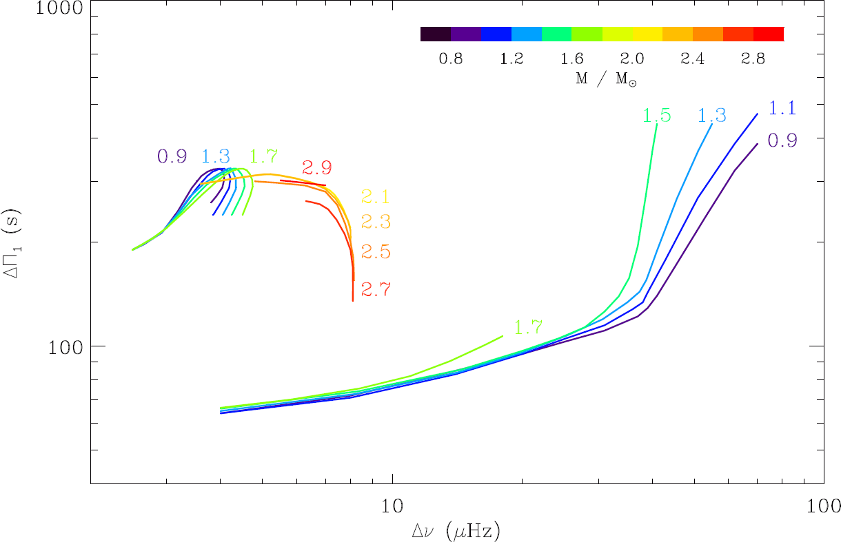
5.5.1 Evolutionary tracks

Stellar evolutionary tracks can be drawn in the $\Delta\Pi_{1}-\Delta\nu$ diagram based on the observation of the large separations and period spacings, derived from the asymptotic fit of radial and mixed dipole modes. From Montalbán et al. (2013), we get a theoretical relation between $\Delta\Pi_{1}$ and the core mass (Fig. 49). Ensemble asteroseismology then helps providing a model independent clear picture of stellar evolution (Fig. 50). In this diagram, we benefit from all seismic information:
- stellar masses and radii are derived from the scaling relations,
- the frequency separation provides information on the extent of the envelope,
- the period spacing provides information on the size and status of the core.

So, independent of modelling, we can distinguish various evolutionary stages:

- S (subgiants): the increase of density in the core induces an increase of the $N_{\mathrm{BV}}$ frequency in the core, so that p and g waves can couple efficiently. In this regime, the $\Delta\Pi_{1}-\Delta\nu$ relation still shows a significant mass dependence.

- R (RGB): the RGB regime differs from the subgiant regime. The properties of the stellar interior become increasingly dominated by the physical conditions of the quasi-isothermal degenerate helium core and its surrounding hydrogen-burning shell. Accordingly, the structural properties of the envelope are also related to the core mass, which explains the degeneracy in the $\Delta\Pi_{1}-\Delta\nu$ diagram. The change of regime is defined with an empirical criterion: a subgiant with a mass below 1.5 $M_{\odot}$ starts climbing the RGB when $(\Delta\nu/36.5\,\mu\hbox{Hz})^{2.5}\,(\Delta\Pi_{1}/126\,\hbox{s})<1$ . The determination of this threshold is better than 8 %. Translated into a stellar age, this uncertainty represents a very short event, much less than 0.5 % of the evolution time on the main sequence.

- C (red clump): red-clump stars occupy a small region of the $\Delta\Pi_{1}-\Delta\nu$ diagram, around 300 s and 4.1 $\mu$ Hz. They have similar core masses, hence similar luminosities, and are therefore used as standard candles. Seismic information provides useful constraints for improving the fine structure of the red clump, hence for improving distance measurements. Models still have difficulties at reproducing the period spacing in the red clump (Bildsten et al., 2012; Montalbán et al., 2013; Stello et al., 2013), in part because they do not consider properly the extra mixing required in the core (Noels & Montalbán, 2013). Now, the accuracy of the measurements of $\Delta\nu$ and $\Delta\Pi_{1}$ is high enough to track the evolution of the stars in the helium-burning phase. Low-mass stars have lower $\Delta\nu$ than more massive stars, hence lower mean density. This is in agreement with the fact that the inner pressure is fixed by the hydrogen shell that produces the largest part of the stellar luminosity. During the first stage of helium burning, the core grows in mass and expands, so that the envelope contracts: both $\Delta\Pi_{1}$ and $\Delta\nu$ increase. In a second stage, both decrease. This evolution is qualitatively predicted by models (Lagarde et al., 2012; Montalbán et al., 2013; Stello et al., 2013).

- 2 (secondary clump): in stars with masses above about $1.9\,M_{\odot}$ , the ignition of helium occurs gradually rather than in a flash because the core is not fully degenerate (Girardi, 1999; Huber et al., 2012; Miglio et al., 2012). Therefore, these secondary-clump stars show a larger spread in the $\Delta\Pi_{1}-\Delta\nu$ diagram (Bildsten et al., 2012): $\Delta\Pi_{1}$ decreases with increasing stellar mass up to 2.7 $M_{\odot}$ , as does the mass of the helium core at ignition. Then, for masses above 2.8 $M_{\odot}$ , $\Delta\Pi_{1}$ increases significantly with increasing stellar mass. This behavior is expected from stellar modelling, which however often fails at reproducing the stellar mass corresponding to the minimum $\Delta\Pi_{1}$ values (Stello et al., 2013, Fig. 51, ).

- A (stars leaving the red clump moving towards the AGB): a few stars appear in the vicinity of the clump, but with significantly smaller period spacings. They most probably correspond to stars in which the core is contracting due to helium becoming exhausted, leaving the main region of the red clump and preparing to ascend the AGB (Lagarde et al., 2012; Corsaro et al., 2012; Montalbán & Noels, 2013). An empirically threshold can be defined: a star leaves the red clump and enters this stage when its large separation is 15 % below the mean value observed in the clump for stars with comparable masses. For low-mass stars, this occurs when $(\Delta\nu/3.3\,\mu\hbox{Hz})^{1.5}\,(\Delta\Pi_{1}/245\,\hbox{s})<1$ .

Other evolutionary stages are identified:

- p2 (pre-secondary clump): it is possible to define, for each mass range, the p2 status, corresponding to progenitors of secondary-clump stars. Progenitors of secondary clump stars have a lower $\Delta\nu$ (a higher luminosity) than the median stage in each mass interval, and also a low $\Delta\Pi_{1}$ corresponding to an extended inner radiative region.

- f (helium flash stage): a small number of stars are clearly outside the evolutionary paths mentioned above. Such stars may have very recently undergone the helium flash. At low $\Delta\nu$ , we identify stars with an unusually high period spacing, corresponding to a small inner radiative region. This situation matches an helium subflash (Bildsten et al., 2012).

The evolutionary tracks are summarized in Fig. 52. Observations reported in Fig. 50 were used to draw these tracks, for 0.2- $M_{\odot}$ mass steps. Finally, stars can also be represented in the classical HR diagram (Fig. 53, where a few main-sequence stars have been included).

5.5.2 Core rotation

The asymptotic analysis of mixed modes provides also their rotational splittings, from which it is possible to derive the mean core rotation (Section 10.3). Rotational splittings have been first observed in a handful of red giants, putting in evidence a significant radial differential rotation (Beck et al., 2012; Deheuvels et al., 2012). Then, Mosser et al. (2012c) have developed a dedicated method for automated measurements of the rotational splittings in a large number of red giants. Their study provides the largest set of core rotational splittings available up to now.

Under the assumption that a linear analysis can provide the rotational splitting, Goupil et al. (2013) have provided an asymptotic description of the rotational splittings, which is operating for both subgiants and red giants. They have proven that the mean core rotation dominates the splittings, even for pressure dominated mixed modes. For red giant stars with slowly rotating cores, the variation in the rotational splittings of dipole modes with frequency depends only on the large frequency separation, the g-mode period spacing, and the ratio of the average envelope to core rotation rates. Thus, they have proposed a method to infer directly this ratio from the observations and have validated this method using Kepler data. In case of rapid rotation, rotation cannot be considered as a perturbation any more and the linear approach fails (Ouazzani et al., 2013).

Mosser et al. (2012c) note a small increase of the mean core rotation period of stars ascending the RGB (Fig. 54). Alternatively, an important spinning down is observed for red-clump stars compared to the RGB. They also show that, at fixed stellar radius, the specific angular momentum increases with increasing stellar mass. Similar observations conducted in subgiants do not show the same trend (Deheuvels et al., 2014). It seems that the spinning-down mechanism occurring on the RGB is not efficient enough in subgiants, as recently explained Belkacem et al. (2015b); Belkacem et al. (2015a).

For investigating the internal transport and surface loss of the angular momentum of oscillating solar-like stars, Marques et al. (2013) have studied the evolution of rotational splittings from the pre-main sequence to the red-giant branch (RGB) for stochastically excited oscillation modes. They have shown that transport by meridional circulation and shear turbulence cannot explain the observed spin-down of the mean core rotation. They suspect the horizontal turbulent viscosity to be largely underestimated.

6 Conclusion

After the study of adiabatic oscillations, it is necessary to investigate non-adiabatic conditions and to enter stellar and Galactic physics in detail, as proposed in the next chapters.

Observations with the CoRoT and Kepler missions are completed, but much more result is to come and forthcoming missions, as K2, TESS, and Plato, will provide new data. In a near future, calibrated scaling relations combined with spectrometric, interferometric and astrometric measurements will boost ensemble asteroseismology. GAIA results, when available, will add new constraints on stellar populations. In parallel, precise stellar modeling based on seismic data makes continuing progress. Seismology has become a fruitful partner of stellar physics!

\Appendix

7 Spherical harmonics

Spherical harmonics are the normal basis for a spherically symmetric problem: hydrogen atom, cosmic microwave background, or stellar interior structure… They are defined by

Y_{\ell}^{m}(\theta,\varphi)\ \stackrel{{\scriptstyle\mathrm{def}}}{{=}}\ (-1)^{(m+|m|)/2}\ \left[{2\ell+1\over 4\pi}{(\ell-|m|)!\over(\ell+|m|)!}\right]^{1/2}P_{\ell}^{|m|}(\cos\theta)\exp im\varphi,

(243)

where the degree $\ell$ is the number of nodal lines, and the azimuthal order $m$ is the number of meridional nodal lines (Figs. 55 and 56). The number of sectors corresponds to to $2m$ ; $\ell-|m|$ gives the number of nodal lines parallel to the equator.

Spherical harmonics are based on the Legendre polynomials $P_{\ell}^{m}(\cos\theta)$ , which are the generic solutions of the differential equation

{{\rm d}\over{\rm d}x}\left[(1-x^{2}){{\rm d}F(\theta)\over{\rm d}x}\right]+\left(L^{2}-{m^{2}\over 1-x^{2}}\right)F(\theta)\ =\ 0,

(244)

with $x=\cos\theta$ . These solutions converge only when $L^{2}=\ell(\ell+1)$ , where $\ell$ and $m$ have integer values, and $m$ is in the range $-\ell$ et $+\ell$ .

Even if spherical harmonics form an orthogonal basis over the full sphere,

\int_{\mathrm{sphere}}Y_{\ell}^{m}.Y_{\ell^{\prime}}^{m^{\prime}}\ {\rm d}\Omega\ =\ \int_{\mathrm{sphere}}Y_{\ell}^{m}.Y_{\ell^{\prime}}^{m^{\prime}}\ \sin\theta{\rm d}\theta{\rm d}\varphi\ =\ \delta_{\ell,\ell^{\prime}}\ \delta_{m,m^{\prime}},

(245)

observations are never able to see the full sphere. On an hemisphere, with limb darkening, orthogonality is not ensured:

\int_{\mathrm{hemisphere}}Y_{\ell}^{m}.Y_{\ell^{\prime}}^{m^{\prime}}\ \sin\theta{\rm d}\theta{\rm d}\varphi\ \neq\ \delta_{\ell,\ell^{\prime}}\ \delta_{m,m^{\prime}},

(246)

so that observations are affected by a confusion between the $(\ell,m)$ values. The main confusion occurs between $(\ell,m)$ and $(\ell\pm 2,m)$ . This may be problematic for observations (Gaulme et al., 2011, e.g.,).

Spherical harmonics are introduced in the components of the wave displacement ${\bm{\xi}}$ projected on the spherical basis:

{\bm{\xi}}(r,\theta,\varphi,t)=\hbox{Re}\left[\hbox{\rm e}^{i{\omega_{n,\ell}}t}\ \left(\xi_{\mathrm{r}}(r)Y_{\ell}^{m}{\bf e}_{\mathrm{r}}+\xi_{\mathrm{h}}(r)\left[{\partial Y_{\ell}^{m}\over\partial\theta}{\bf e}_{\theta}+{1\over\sin\theta}{\partial Y_{\ell}^{m}\over\partial\varphi}{\bf e}_{\varphi}\right]\right)\right].

(247)

The degree $\ell$ and azimuthal order $m$ are connected with the spherical angles $\theta$ et $\varphi$ , respectively, as the cyclic frequency $\nu$ is connected with time $t$ .

The quantization expressed by the degree $\ell$ comes from the relation

\nabla_{\mathrm{h}}^{2}\ Y_{\ell}^{m}\ =\ -{\ell(\ell+1)\over r^{2}}\ Y_{\ell}^{m},

(248)

where $\nabla_{\mathrm{h}}$ is the horizontal gradient. This relation, crucial for the seismic study, derives from the generic properties of the functions $f$ with separate angular variables $\theta$ et $\varphi$ ( $f(\theta,\varphi)=f_{1}(\theta)f_{2}(\varphi)$ ), which obey the Laplace relation

\nabla^{2}_{\mathrm{h}}\ f\ =\ -{1\over r^{2}}\ L^{2}f

(249)

where $L$ is a constant term. This equation can be developed as:

{1\over\sin\theta}{\partial\over\partial\theta}\left(\sin\theta{\partial f\over\partial\theta}\right)+{1\over\sin^{2}\theta}{\partial^{2}f\over\partial\varphi^{2}}\ =\ -L^{2}\ f

(250)

and provides the basis of the characteristic differential equation defining the Legendre polynomials.

The quantization expressed by Eq. (248) corresponds to a key relation for the horizontal wavenumber:

k_{\mathrm{h}}\ =\ {\sqrt{\ell(\ell+1)}\over r}.

(251)

Finally, an obvious property of the angular derivative with respect to $\varphi$ is

{\partial Y_{\ell}^{m}\over\partial\varphi}=m\ Y_{\ell}^{m}.

(252)

This explains the main term of the rotational splitting (Eq. 291).

8 Derivation of the asymptotic expression

In the section, we follow the analysis of Tassoul (1980), hereafter T80.

8.1 Eigenfunctions and eigenfrequencies

Following the JWKB analysis, the linearized equations governing the low-degree adiabatic oscillations are developed, as functions of a large parameter, namely the frequency. Near the internal and external turning points, respectively the center and the upper troposphere, the pressure perturbation and the radial eigendisplacement are expressed in terms of Bessel functions.

The Bessel functions are characteristic solutions of the differential equation

x^{2}{{\rm d}^{2}y\over{\rm d}x^{2}}+x{{\rm d}y\over{\rm d}x}+(x^{2}-\alpha^{2})\;y=0.

(253)

In a spherical problem, the order $\alpha$ has half-integer value $(\alpha=\ell+1/2)$ . The Bessel functions are developed to the second order in the argument $\omega$ , where $\omega=2\pi\nu$ and $\tau$ is some characteristic time, in the following way:

J_{\alpha}(\omega\tau)\ =\ \sqrt{2\over\pi\omega\tau}\ \left[\cos\chi-{4\alpha^{2}-1\over 8\omega\tau}\sin\chi\right],

(254)

with $\chi\ =\ \omega\tau-\alpha\pi/2-\pi/4$ . The development is valid as soon as the argument $\omega\tau$ satisfies the relation

\omega\tau\ \gg\ (4\alpha^{2}-1)(4\alpha^{2}-9)/128.

(255)

For a pressure mode of degree $\ell$ , the expressions of the radial eigendisplacements and the Lagrangian pressure perturbations, developed up to the second order in frequency, are combinations of the Bessel functions $J_{\ell+1/2}$ and $J_{\ell+3/2}$ in the central region and $J_{n_{o}}$ and of $J_{n_{o}+1}$ in the envelope. We use Lagrangian perturbations in order to treat possible discontinuities, as for instance in the presence of a dense core, or in the region of second ionization of helium.

When the condition given by Eq. (255) is fulfilled, one writes for pressure modes (Provost et al., 1993, T80,):

$\displaystyle(\delta p)_{i}$	$\displaystyle\propto$	$\displaystyle{\sqrt{\rho c}\over r}\left[\cos\phi_{i}-\left\{F_{i}+{\ell(\ell+1)\over 2\tau_{i}(r)}-{g\over c}\right\}{\sin\phi_{i}\over\omega}\right]$	(256)
$\displaystyle\xi_{i}$	$\displaystyle\propto$	$\displaystyle-{\omega^{-1}\over r\sqrt{\rho c}}\left[\sin\phi_{i}+\left\{H_{i}+{\ell(\ell+1)\over 2\tau_{i}(r)}\right\}{\cos\phi_{i}\over\omega}\right]$	(257)
$\displaystyle(\delta p)_{o}$	$\displaystyle\propto$	$\displaystyle-{\sqrt{\rho c}\over r}\left[\sin\phi_{o}\vphantom{{H_{o}\tau_{o}(r)\over 2}}\right.+\left.{\left\{{H_{o}\tau_{o}(r)\over 2}{4n_{o}^{2}-5\over 8\tau_{o}(r)}+{g\over c}\right\}}{\cos\phi_{o}\over\omega}\right]$	(258)
$\displaystyle\xi_{o}$	$\displaystyle\propto$	$\displaystyle{\omega^{-1}\over r\sqrt{\rho c}}\left[\cos\phi_{o}-\left\{{2F_{o}\over\tau_{o}(r)}+{4n_{o}^{2}-1\over 8\tau_{o}(r)}\right\}{\sin\phi_{o}\over\omega}\right]$	(259)

The amplitude factors have been omitted. The index $i$ and $o$ refer, respectively, to quantities in the central region and in the envelope. All the symbols which are here not defined have the same signification as in T80. The expressions derive from the developments of Bessel functions (in the inner region, $J_{\ell+1/2}$ for the pressure perturbation, $J_{\ell+3/2}$ for the displacement).

The two phases $\phi_{i}$ and $\phi_{o}$ , respectively related to propagation in the central region and in the envelope, are

	$\displaystyle\phi_{i}$	$\displaystyle=$	$\displaystyle\omega\tau_{i}-(\ell+1/2)\ {\pi\over 2}-{\pi\over 4},$		(260)
	$\displaystyle\phi_{o}$	$\displaystyle=$	$\displaystyle\omega\tau_{o}-n_{o}\,{\pi\over 2}-{\pi\over 4},$		(261)

with

\tau_{i}(r)\,=\int_{0}^{r_{io}}\!{{\rm d}r\over c}\hbox{ \ and \ }\tau_{o}(r)\,=\int_{r_{io}}^{R}\!{{\rm d}r\over c}.

(262)

$\tau_{i}$ and $\tau_{o}$ are the values of $\tau_{i}(r_{io})$ and $\tau_{o}(r_{io})$ at the boundary $r_{io}$ where solutions will be connected. The expression of the eigenfrequency is obtained by assuming the continuity of $\delta p$ and $\xi$ at the boundary.

In the general case without structure discontinuity, the exact location $r_{io}$ of the boundary plays no role so that the validity of the development ensures that the value of $r_{io}$ finally disappears. In case of a density or sound-speed discontinuity, $r_{io}$ is chosen at the frontier. Then:

\varrho\varsigma\ ={(\rho c)_{i}\over(\rho c)_{o}}

(263)

is different from 1. The index $i$ and $o$ refer now, respectively, to quantities estimated at the boundary. For an intensive variable $x$ , $x_{i}$ is necessarily equal to $x_{o}$ , but extensive parameters may have different values on the inner and outer side of the boundary.

The implicit calculation of the eigenfrequencies is then given by

$\displaystyle\varrho\varsigma\$	$\displaystyle\left[\cos\phi_{i}-\omega^{-1}\left\{F_{i}+\displaystyle{\ell(\ell+1)\over 2\tau_{i}}-\displaystyle{g\over c_{i}}\right\}\sin\phi_{i}\right]$	(264)
	$\displaystyle\left[\cos\phi_{o}-\omega^{-1}\left\{F_{o}\displaystyle{2\over\tau_{o}}+\displaystyle{4n_{o}^{2}-1\over 8\tau_{o}}\right\}\sin\phi_{o}\right]$
$\displaystyle=$	$\displaystyle\left[\sin\phi_{i}+\omega^{-1}\left\{H_{i}+\displaystyle{\ell(\ell+1)\over 2\tau_{i}}\right\}\cos\phi_{i}\right]$
	$\displaystyle\left[\sin\phi_{o}+\omega^{-1}\left\{H_{o}\displaystyle{\tau_{o}\over 2}+\displaystyle{4n_{o}^{2}-5\over 8\tau_{o}}+\displaystyle{g\over c_{o}}\right\}\cos\phi_{o}\right].$

When the terms varying as $\omega^{-1}$ are supposed to be small (which is not a priori satisfied if the inner turning point is deep), this implicit relation leads to the following explicit form of the dispersion equation:

\cos(\theta_{i}+\theta_{o})\ =\ -\eta\ \cos(\theta_{i}-\theta_{o})

(265)

where $\eta$ is the ratio $(\varrho\varsigma-1)/(\varrho\varsigma+1)$ . The values of $\theta_{i}$ and $\theta_{o}$ can be derived from Eqs. (256) to (259) at the first and second orders in $\omega^{-1}$ . Let us note that in the continuous case $\eta=0$ , we recover Tassoul’s solution for the eigenfrequency, up to the second order in frequency.

8.2 First-order terms

To the first order in frequency, ${\theta_{i}}^{(1)}$ and ${\theta_{o}}^{(1)}$ identify to

	$\displaystyle{\theta_{i}}^{(1)}$	$\displaystyle=$	$\displaystyle\phi_{i}$		(266)
	$\displaystyle{\theta_{o}}^{(1)}$	$\displaystyle=$	$\displaystyle\phi_{o}$		(267)

and the phase combinations of Eq. (265) are

	$\displaystyle{\theta_{i}}^{(1)}+\theta_{o}^{(1)}$	$\displaystyle=$	$\displaystyle\omega(\tau_{i}+\tau_{o})-\ell{\pi\over 2}-n_{o}{\pi\over 2}-{3\pi\over 4}$		(268)
	$\displaystyle{\theta_{i}}^{(1)}-\theta_{o}^{(1)}$	$\displaystyle=$	$\displaystyle\omega(\tau_{i}-\tau_{o})-\ell{\pi\over 2}+n_{o}{\pi\over 2}-{\pi\over 4}.$		(269)

The solution in the continuous case ( $\eta=0$ ) writes

\theta_{i}+\theta_{o}\ =\ {\pi\over 2}+p\pi\quad(p\in\mathrm{I\!N}).

(270)

Since $\eta$ is small we search the solution of Eq. (265) at the first order in frequency as a perturbation $\delta\omega$ of the solution of Eq. (270). The development of Eq. (265) gives the first-order expression of the eigenfrequency and leads to the development of the second-order solution in $\eta$ .

8.3 Second-order terms

Obtaining symmetric phases after the expansion of the condition of continuity introduces a correction to the second-order coefficients of T80. The new phases $\theta_{i}$ and $\theta_{o}$ that appear in Eq. (265) are then, including the second-order corrections $\varphi_{i}$ and $\varphi_{o}$ :

$\displaystyle\theta_{i}{}^{(2)}$	$\displaystyle=$	$\displaystyle\phi_{i}-\omega^{-1}\Biggl\{{1\over 2}\Bigl(F_{i}+H_{i}-{\ell(\ell+1)\over\tau_{i}}$	(271)
	$\displaystyle-$	$\displaystyle{g\over c_{i}}+\eta T_{i}+{2\varrho\varsigma\over\varrho\varsigma+1}{T_{i}-T_{o}\over\varrho\varsigma-1}\Bigr)\Biggr\}$
	$\displaystyle=$	$\displaystyle\phi_{i}-\omega^{-1}\varphi_{i}$
$\displaystyle\theta_{o}{}^{(2)}$	$\displaystyle=$	$\displaystyle\phi_{o}-\omega^{-1}\Biggl\{{1\over 2}\Bigl({2F_{o}\over\tau_{o}}+{H_{o}\tau_{o}\over 2}+{4n_{o}^{2}-3\over 4\tau_{o}}$	(272)
	$\displaystyle+$	$\displaystyle{g\over c_{o}}+\eta T_{o}-{2\varrho\varsigma\over\varrho\varsigma+1}{T_{i}-T_{o}\over\varrho\varsigma-1}\Bigr)\Biggr\}$
	$\displaystyle=$	$\displaystyle\phi_{o}-\omega^{-1}\varphi_{o}$

The functions $F$ and $H$ are expressed in T80. The terms $T_{i}$ and $T_{o}$ are respectively

T_{i,o}\ =\ {c_{i,o}\over 2}\left[\ {1\over\rho}{{\rm d}\rho\over{\rm d}r}+{1\over c}{{\rm d}c\over{\rm d}r}-{2\over r}\ \right]_{i,o}.

(273)

First, the function $T$ differs from its expression in T80 because of taking account for the Lagrangian perturbation. Second, the values of $T_{i}$ and $T_{o}$ may differ at the frontier because of the discontinuity. This difference induces then discontinuous terms related to the density and sound-speed jumps at the boundary. The functions $F$ and $H$ , principally given by the integration of the term $\Omega_{2}$ of T80, give the second-order coefficient in term of density and sound speed scale heights. If we introduce two parameters, $\psi_{i}$ and $\psi_{o}$ , which represent the two integrals of Eq. (66) in T80, the family of the second-order constants $V$ expresses by

$\displaystyle L^{2}V_{1}\ +\ V_{2}$	$\displaystyle=$	$\displaystyle 2\,(\varphi_{i}+\varphi_{o})$	(274)
	$\displaystyle=$	$\displaystyle\left({\psi}_{i}+{\psi}_{o}\right)+3g\left({1\over c_{i}}-{1\over c_{o}}\right)+2\ (T_{i}-T_{o})-\eta\ (T_{i}+T_{o})$	(274)
$\displaystyle L^{2}V_{3}\ +\ V_{4}$	$\displaystyle=$	$\displaystyle 2\ \left[{\tau_{o}\over\tau_{o}+\tau_{i}}\varphi_{i}-{\tau_{i}\over\tau_{o}+\tau_{i}}\varphi_{o}\right]$	(275)
	$\displaystyle=$	$\displaystyle{\tau_{o}\over\tau_{o}+\tau_{i}}\left[\psi_{i}+{3g\over c_{i}}+(2-\eta)T_{i}-{2\varrho\varsigma\over\varrho\varsigma+1}{T_{i}-T_{o}\over\varrho\varsigma-1}\right]$	(275)
	$\displaystyle-$	$\displaystyle{\tau_{i}\over\tau_{o}+\tau_{i}}\left[\psi_{o}-{3g\over c_{o}}-(2+\eta)T_{o}+{2\varrho\varsigma\over\varrho\varsigma+1}{T_{i}-T_{o}\over\varrho\varsigma-1}\right].$	(276)

The values of $\varphi_{i}$ and $\varphi_{o}$ are derived from Eq. (275) and are used to calculate the implicit asymptotic values, with Eqs. (265), (271) and (272). If we further assume that the interior is a fully convective polytrope, characterized by the adiabatic coefficients $\Gamma_{i}$ in the central region and $\Gamma_{o}$ in the outer region, we may calculate the functions $\psi_{i}$ and $\psi_{o}$ , derived from the function $\Omega_{2}$ of T80:

$\displaystyle\psi_{i}$	$\displaystyle=$	$\displaystyle L^{2}\left[\int_{0}^{r_{i}}\!\!{{\rm d}c\over r}-{c_{i}\over r}\right]+{1\over 4}\left({\Gamma_{i}-3\over\Gamma_{i}-1}\right)^{2}\int_{0}^{r_{i}}\!\!{1\over M}{{\rm d}M\over{\rm d}r}{\rm d}c$	(277)
	$\displaystyle+$	$\displaystyle{1\over 2}\left[{4\over\Gamma_{i}-1}-\left({\Gamma_{i}-3\over\Gamma_{i}-1}\right)^{2}\right]\int_{0}^{r_{i}}\!\!{{\rm d}c\over r}+{(\Gamma_{i}-3)(3\Gamma_{i}-5)\over 8(\Gamma_{i}-1)}{g\over c_{i}}$	(277)
$\displaystyle\psi_{o}$	$\displaystyle=$	$\displaystyle L^{2}\left[\int_{r_{o}}^{R}\!\!{{\rm d}c\over r}+{c_{o}\over r}\right]+{1\over 4}\left({\Gamma_{o}-3\over\Gamma_{o}-1}\right)^{2}\int_{r_{o}}^{R}\!\!{1\over M}{{\rm d}M\over{\rm d}r}{\rm d}c$	(278)
	$\displaystyle+$	$\displaystyle{1\over 2}\left[{4\over\Gamma_{o}-1}-\left({\Gamma_{o}-3\over\Gamma_{o}-1}\right)^{2}\right]\int_{r_{o}}^{R}\!\!{{\rm d}c\over r}-{(\Gamma_{o}-3)(3\Gamma_{o}-5)\over 8(\Gamma_{o}-1)}{g\over c_{o}}$	(278)

where $M$ is the mass inside the sphere of radius $r$ . Continuity of the solution implies $r_{i}=r_{o}$ at the boundary $r_{b}$ . The term $V_{1}$ becomes simply:

V_{1}\ =\ \left[\int_{0}^{r_{b}}\!{{\rm d}c\over r}+\int_{r_{b}}^{R}\!{{\rm d}c\over r}\right]\ +\ \left({\Delta c\over r}\right)_{\mathrm{\small{boundary}}}\ =\ \int_{0}^{R}\!{{\rm d}c\over r}

(279)

In case of discontinuity of the sound-speed profile at $r_{b}$ , the term $(\Delta c/r)_{\mathrm{\small{boundary}}}$ may correct severely the negative contribution of the integral. In case of non-adiabaticity, all previous equations which lead to the expression of the 2^nd order terms $V$ remain valid, except the ones which give $\psi_{i}$ and $\psi_{o}$ , which have to be changed according to Eq. (68) of T80.

8.4 Implicit asymptotic expression

The implicit expression is obtained when denying the factorization of the sinus and cosinus in Eqs. (256) to (260), which supposes that the terms in $\omega^{-1}$ are small. Then, with $\psi_{i}^{\prime}=\psi_{i}+3g/c_{i}$ and $\psi_{o}^{\prime}=\psi_{o}-3g/c_{o}$ , the continuity of the eigenfunctions at the boundary expresses by

$\displaystyle\varrho\varsigma$	$\displaystyle\left[\cos\phi_{i}+{1\over 2\omega}(\psi_{i}^{\prime}+\hphantom{3}T_{i})\sin\phi_{i}\right]$	(280)
	$\displaystyle\left[\cos\phi_{o}+{1\over 2\omega}(\psi_{o}^{\prime}-3T_{o})\sin\phi_{o}\right]$
$\displaystyle=$	$\displaystyle\left[\sin\phi_{i}-{1\over 2\omega}(\psi_{i}^{\prime}+3T_{i})\cos\phi_{i}\right]$
	$\displaystyle\left[\sin\phi_{o}-{1\over 2\omega}(\psi_{o}^{\prime}-\hphantom{3}T_{o})\cos\phi_{o}\right].$

The second-order coefficients are increasing functions of $\ell$ , as indicated by Eqs. (277) and (278). The difference with the continuous case lies in the terms $g/c_{i}$ and $g/c_{o}$ , $T_{i}$ and $T_{o}$ , as well as in the terms $L^{2}\thinspace c_{i}/r$ and $L^{2}\thinspace c_{o}/r$ implying the $\ell$ dependence.

9 Variational principle

Adiabatic oscillations can be seen as an eigenvalue problem in an Hilbert space. Hilbert spaces can be considered as extensions of the Euclidean space, in the sense they offer many mathematical properties derived from the usual Euclidean space to any spaces with any dimensions. Spectral methods in an Hilbert space are used to study the behavior of eigenvalues and eigenfunctions of differential equations.

The equation of motion (Eq. 3) can be rewritten with an operator ${\cal L}$

$\displaystyle{\cal L}({\bm{\xi}})$	$\displaystyle=$	$\displaystyle{1\over\rho_{0}^{2}}\nabla p_{0}\nabla.(\rho_{0}{\bm{\xi}})-{1\over\rho_{0}}\nabla\bigl(\nabla p_{0}.{\bm{\xi}}\bigr)-{1\over\rho_{0}}\nabla\bigl(c^{2}\rho_{0}\nabla{\bm{\xi}}\bigr)$
		$\displaystyle\ +\nabla\left[{\cal G}\int{\nabla.(\rho_{0}{\bm{\xi}})\ {\rm d}\textthreesuperior{\bf x}\over\Bigl\|{\bf x}-{\bf r}\Bigr\|}\right]$
	$\displaystyle=$	$\displaystyle\ \omega^{2}{\bm{\xi}},$

where $\omega$ is introduced by the time dependence $\partial/\partial t\equiv i\omega$ of the spectral method.

The Hilbert multidimensional space possesses the structure of an inner product defined by

\langle x,y\rangle=\int\rho x^{\star}\cdot y\ {\rm d}\textthreesuperior{\bf r},

(281)

where ^⋆ is the complex conjugate. The operator is symmetric:

\langle x,{\cal L}(y)\rangle=\langle{\cal L}(x),y\rangle.

(282)

Eigenvalues of the operator ${\cal L}$ are given by this inner product

\omega_{n,\ell}^{2}\ =\ {{\displaystyle\int{\bm{\xi}}_{n,\ell}^{\star}\cdot{\cal L}({\bm{\xi}}_{n,\ell})\ \rho_{0}\ {\rm d}\textthreesuperior{\bf r}}\over{\displaystyle\int{\bm{\xi}}_{n,\ell}^{\star}\cdot{\bm{\xi}}_{n,\ell}\ \rho_{0}\ {\rm d}\textthreesuperior{\bf r}}},

(283)

which is the spirit of the Hilbert space. The variational principal shows that a small change in the interior model implies:
- a change $\delta{\cal L}$ of the Hilbertian operator,
- a change $\delta\omega^{2}_{n,\ell}$ of the eigenvalues,
- but no change, at first order, of the eigenfunctions ${\bm{\xi}}_{n,\ell}$ .

A model can be used to infer the eigenvalues $\omega_{n,\ell}$ and eigenfunctions ${\bm{\xi}}_{n,\ell}$ . The comparison of the observed and modelled frequencies helps determining
- the frequency differences $\delta\omega^{2}_{n,\ell}$ ,
- the difference $\delta{\cal L}$ , since ${\bm{\xi}}_{n,\ell}$ are known from the synthetic model,
according to

\delta\omega_{n,\ell}^{2}\ =\ {\langle{\bm{\xi}}_{n,\ell},\delta{\cal L}({\bm{\xi}}_{n,\ell})\rangle_{\ell}\over\langle{\bm{\xi}}_{n,\ell},{\bm{\xi}}_{n,\ell}\rangle_{\ell}}\ =\ {{\displaystyle\int{\bm{\xi}}_{n,\ell}^{\star}\cdot\delta{\cal L}({\bm{\xi}}_{n,\ell})\ \rho_{0}\ {\rm d}\textthreesuperior{\bf r}}\over{\displaystyle\int{\bm{\xi}}_{n,\ell}^{\star}\cdot{\bm{\xi}}_{n,\ell}\ \rho_{0}\ {\rm d}\textthreesuperior{\bf r}}}.

(284)

So,

{\delta\omega_{n,\ell}\over\omega_{n,\ell}}\ =\ {{{1\over 2}}}\ {\delta\omega_{n,\ell}^{2}\over\omega_{n,\ell}^{2}}\ =\ {1\over 2\omega_{n,\ell}^{2}}\ {\langle{\bm{\xi}}_{n,\ell},\delta{\cal L}({\bm{\xi}}_{n,\ell})\rangle_{\ell}\over\langle{\bm{\xi}}_{n,\ell},{\bm{\xi}}_{n,\ell}\rangle_{\ell}}.

(285)

We infer the linear variation of the operator with the kernels $K^{n,\ell}_{\mathrm{X}}$ that measure the influence of the variable $Z$ on the eigenvalue $\omega_{n,\ell}$

{\delta\omega_{n,\ell}\over\omega_{n,\ell}}\ =\ \int_{0}^{R}\left[K_{\mathrm{c^{2}}}^{n,\ell}(r){\delta c^{2}\over c^{2}}+K_{\mathrm{\rho}}^{n,\ell}(r){\delta\rho\over\rho}+K_{\mathrm{X}}^{n,\ell}(r){\delta Z\over Z}\right]\ {\rm d}r.

(286)

This relations is of great use in asteroseismology since it allows improving the match of the model to the observed data. One often uses weighted kernels, able to probe a given region of the stellar interior (Fig. 57).

10 Rotation

Rotation was always neglected in what precedes. We may investigate its action as a perturbation of the non-rotating case. In case of rapid rotation, a perturbative approach is not convenient and one has to consider a direct approach that takes the centrifugal distortion into account (Ouazzani et al., 2013, e.g.,). This is beyond the scope of this lecture.

The introduction of rotation into the equation of motion introduces the non-galilean terms expressing the Coriolis and centrifugal contributions. It also introduces the difference between the rotation frame where the star does not rotate and the frame of the observer.

The eigensolutions are perturbed in the following way (Aerts et al., 2010):

\delta\omega=-i\ {\displaystyle{\int\rho_{0}{\bm{\xi}}^{\star}(\mathbf{v_{0}}.\mathbf{\nabla}){\bm{\xi}}\ {\rm d}\textthreesuperior{\bf r}}\over\displaystyle{\int\rho_{0}|{\bm{\xi}}|^{2}\ {\rm d}\textthreesuperior{\bf r}}}.

(287)

If the rotation profile is smooth enough so that a linear approach makes sense, it is possible define a mean rotation value by

\langle\Omega\rangle={\int\Omega\ |{\bm{\xi}}|^{2}\ \rho_{0}{\rm d}\textthreesuperior{\bf r}\over\int|{\bm{\xi}}|^{2}\ \rho_{0}{\rm d}\textthreesuperior{\bf r}}.

(288)

For mixed modes, we have seen that the displacement associated with a mode strongly depends on the density and sound speed, since the density of kinetic energy is approximately conserved (Eq. 197). So the previous equation is equivalent to

\langle\Omega\rangle_{p}\simeq{\int\Omega\ {\rm d}\tau\over\int{\rm d}\tau}\simeq 2\Delta\nu\int\Omega{{\rm d}r\over c},

(289)

if we assume that the variation in $\Omega$ are dominated by radial gradients. This means that the mean value of the rotation profile for pressure modes is heavily weighted by the inverse of the sound speed. In other words, stellar rotation as seen by the pressure modes is mostly probed in the outer stellar envelope only.

For gravity modes, the situation can be inferred by analogy. Instead of having the mean rotation weighted by the acoustic radius, the integration takes the buoyancy radius into account

\langle\Omega\rangle_{g}\simeq{\displaystyle\int\Omega\ N_{\mathrm{BV}}\ \displaystyle{{\rm d}r\over r}\over\displaystyle\int N_{\mathrm{BV}}\ \displaystyle{{\rm d}r\over r}}.

(290)

10.1 Axisymmetrical case

With the reasonable hypothesis of axisymmetry, we suppose that $\Omega=\Omega(r,\theta)$ . We can then perturb the normal mode approach, with a new specification: the symmetry axis of the spherical harmonics is defined by the stellar rotation axis. This introduces the azimuthal order $m$ . In the general case, one uses the eigenfunctions associated with the unperturbed solutions $\omega_{n,\ell}$ . This helps defining the eigenfunctions associated with $\omega_{n,\ell,m}$ , with the $m$ dependence derived from the definition of the spherical harmonics (Eq. 243).

Classical computations give a generic form where all the rotational information is provided by the rotational kernels $K_{n,\ell,m}$ (Aerts et al., 2010):

\omega_{n,\ell,m}\ =\ \omega_{n,\ell}+m\int\!\!\!\!\int K_{n,\ell,m}(r,\theta)\ \Omega(r,\theta)\ r{\rm d}r{\rm d}\theta.

(291)

Having $\omega_{n,\ell,0}=\omega_{n,\ell}$ derives from the assumption of slow rotation. In case rotation is rapid enough for rendering an oblate shape, this is no more the case (Mosser, 1990).

Rotational kernels are useful to map the regions from where rotational information can be inferred (Fig. 58). Since the information is weighted by the travel time of the wave, rotational kernels are mostly sensitive to the external region (Fig. 59).

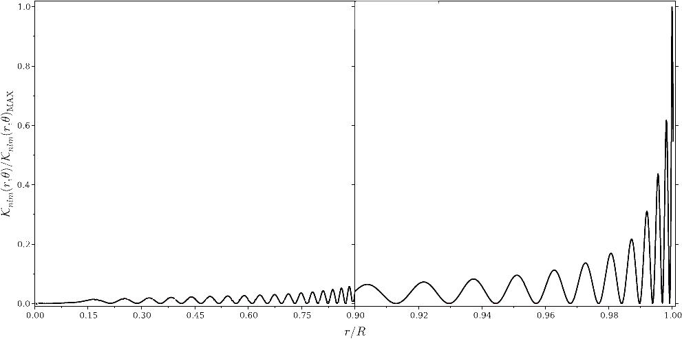
10.2 Spherically symmetric case

Even if differential rotation is largely observed, we may examine the simple case where $\Omega=\Omega(r)$ for two reasons:
- in such a case mathematical manipulations are considerably simplified, so it is possible to emphasize the physics of the phenomenon;
- radial differential rotation is known to be huge in evolved stars (Beck et al., 2012), whereas azimuthal differential rotation is often soft and limited to a few tens percent (Mosser et al., 2009, e.g.,).

Such a rotation profile is called shellular rotation (Zahn, 1992).

According to the definition of the mean rotation (Eq. 288) derived from the perturbation approach, one can write $\delta\omega_{n,\ell,m}=\omega_{n,\ell,m}-\omega_{n,\ell}$ in the form

\delta\omega_{n,\ell,m}=m\ {\displaystyle\int_{0}^{R}\left(\xi_{\mathrm{r}}^{2}+\ell(\ell+1)\xi_{\mathrm{h}}^{2}-2\xi_{\mathrm{r}}\xi_{\mathrm{h}}-\xi_{\mathrm{h}}^{2}\right)\ \rho_{0}\,r^{2}\,\Omega\,{\rm d}r\over\displaystyle\int_{0}^{R}\left(\xi_{\mathrm{r}}^{2}+\ell(\ell+1)\xi_{\mathrm{h}}^{2}\right)\ \rho_{0}\,r^{2}\,{\rm d}r},

(292)

when the rotation depends on $r$ only. This is often abbreviated as

\delta\omega_{n,\ell,m}=m\ \beta_{n,\ell}\ \langle\Omega\rangle,

(293)

or, equivalently, with the Ledoux coefficients,

\delta\omega_{n,\ell,m}=m\ (1-C_{n,\ell})\ \langle\Omega\rangle.

(294)

For dipole modes, the dominating terms in Eq. (292) are $\xi_{\mathrm{r}}^{2}$ and $\ell(\ell+1)\xi_{\mathrm{h}}^{2}$ , so that

\beta_{n,\ell}\simeq 1\ \hbox{ and }\ C_{n,\ell}\simeq 0.

(295)

The splitting is mainly related to the rotating frame, in agreement with the fact that terms introduced by the Coriolis force, in fact measured by $C_{n,\ell,m}$ , are neglected.

For gravity modes, $\xi_{\mathrm{h}}$ dominates in Eq. (292) so that

\beta_{n,\ell}\simeq 1-{1\over\ell(\ell+1)}\ \hbox{ and }\ C_{n,\ell}\simeq{1\over\ell(\ell+1)}.

(296)

For low degree $\ell$ , and especially for dipole modes with $\ell=1$ , the Coriolis force plays a non-negligible role.

10.3 Mixed modes

Measuring rotational splittings of mixed modes is useful for inferring the inner rotation profile in the radiative region. This can be done in $\gamma$ Dor-type stars for instance (Fig. 60). The rotational splittings of mixed modes observed in subgiants and giant stars are described by Goupil et al. (2013). As mixed modes share properties of pressure and gravity modes, their rotational splittings are more or less dominated by the pressure and gravity terms, depending on the mode frequency. As a result, the splittings undergo the mixed influence of the mean core rotation and of the mean envelope rotation (Fig. 61). Of course, one has to suppose that this mean rotation can be defined, which seems confirmed by observations, which show significant spin down with stellar evolution (Mosser et al., 2012b).

These mean rotations are respectively defined by

\langle\Omega\rangle_{\mathrm{core}}=\int_{\mathrm{core}}\Omega(x){N_{\mathrm{BV}}\over x}{\rm d}x\Bigm/\int_{\mathrm{core}}{N_{\mathrm{BV}}\over x}{\rm d}x

(297)

and

\langle\Omega\rangle_{\mathrm{env}}=\int_{\mathrm{env}}\Omega(x){{\rm d}x\over c}\Bigm/\int_{\mathrm{env}}{{\rm d}x\over c},

(298)

where $x=r/R$ is a normalized radius.

The rotational splitting writes

\delta\nu=\beta_{\mathrm{core}}{\langle\Omega\rangle_{\mathrm{core}}\over 2\pi}+\beta_{\mathrm{env}}{\langle\Omega\rangle_{\mathrm{env}}\over 2\pi},

(299)

with

\beta_{\mathrm{env,core}}=\int_{\mathrm{env,core}}K(x){\rm d}x.

(300)

The coefficients $\beta_{\mathrm{core}}$ and $\beta_{\mathrm{env}}$ (Fig. 62) result from the expression of the inertia, assuming shellular rotation, with new variables

	$\displaystyle\mathcal{I}$	$\displaystyle=$	$\displaystyle 4\pi\,r^{3}\ \int_{0}^{1}(\xi r^{2}+\ell(\ell+1)\xi_{\mathrm{h}}^{2})\rho_{0}x^{2}{\rm d}x$		(301)
		$\displaystyle=$	$\displaystyle\int_{0}^{1}(z_{1}^{2}+z_{2}^{2}){{\rm d}x\over x},$		(302)

with

z_{1}^{2}={3\rho_{0}\over\langle\rho_{0}\rangle}\ \left({\xi_{\mathrm{r}}\over R}\right)^{2}\ x^{3}

(303)

and

z_{2}^{2}=\ell(\ell+1)\ {3\rho_{0}\over\langle\rho_{0}\rangle}\ \left({\xi_{\mathrm{h}}\over R}\right)^{2}\ x^{3}.

(304)

The kernel then writes

K={1\over\mathcal{I}}\left(z_{1}^{2}-{2\over\sqrt{\ell(\ell+1)}}\,z_{1}z_{2}+\left(1-{1\over\ell(\ell+1)}\right)z_{2}^{2}\right)\ {1\over x}.

(305)

The variations of $z_{1}$ and $z_{2}$ as a function of $x$ explain that splittings show variations between the mean envelope and core rotations (Fig. 63).

Goupil et al. (2013) have asymptotically developed the function $z_{1}^{2}$ and $z_{2}^{2}$ to obtain an explicit expression of the rotational splitting. The formalism is quite similar to the development used in Section 4.6 for obtaining the asymptotic expansion of mixed modes, so that results are expressed in similar forms. Rotational splittings are expressed by the coefficient

\zeta={1\over 1+\Delta\nu\Delta\Pi_{1}\ \chi^{2}},

(306)

with

\chi\simeq 2{\nu\over\Delta\nu}\ \cos\left({\pi\over\nu\Delta\Pi_{1}}\right).

(307)

The splitting writes

{\delta\nu\over\delta\nu_{\mathrm{max}}}={1-2\mathcal{R}\over 1+\Delta\nu\Delta\Pi_{1}\ \chi^{2}}+2\mathcal{R},

(308)

where $\mathcal{R}=\langle\Omega\rangle_{\mathrm{env}}/\langle\Omega\rangle_{\mathrm{core}}$ is the ratio of the mean rotations in the envelope and in the core, and $\delta\nu_{\mathrm{max}}$ is very close to $\langle\Omega\rangle_{\mathrm{core}}/4\pi$ . The extra 1/2 factor coming in this relation is the Ledoux coefficient of dipole gravity modes (Eq. 296).

Figure 64 compares the splitting observed in an RGB star with the modelling. The determination of the global seismic parameter helps explaining the affine relation with the parameter $\zeta$ . This provides a precise fit of the rotational splittings, where discrepancies are mostly explained by the resolution of the observed peaks.

The factor $\zeta$ in Eq. (306) can be used to analyze the asymmetry in the splitting. In fact, a multiplet near a pressure-dominated mode cannot be symmetric: the splitting of the component $m=\pm 1$ close to the pressure-dominated mode is smaller than the opposite component $m=\mp 1$ .

11 Surface term

11.1 Pressure modes

As shown by its definition (Eq. 146), the asymptotic frequency spacing $\Delta\nu_{\mathrm{as}}$ is heavily weighted by the external region where the sound speed has low values (Fig. 7). However, this region cannot be depicted with the same precision as the inner layers since hypothesis valid in the inner regions are no longer valid. We note :
- the inadequacy of the adiabatic approximation,
- pressure and density scale heights with low values, so that one can no more consider that they are much larger than the wavelength…

We also have seen that the low-frequency waves are reflected in deeper region. Their frequencies are not perturbed by an improper treatment of the uppermost layers, contrary to higher frequencies (Fig. 12). This is a general problem, for instance studied for Jovian seismology (Mosser et al., 1994; Mosser, 1995), which requires the introduction of a surface term for correcting the modelled frequencies before comparison with observed frequencies. In stars, a generic form was proposed by Kjeldsen et al. (2008), varying as

\nu_{\mathrm{obs}}=\nu_{\mathrm{model}}+a\left({\nu\over\nu_{\mathrm{cor}}}\right)^{b},

(309)

where the coefficient $a$ and the exponent $b$ have negative value: high-frequency waves spend more time in the upper atmospheric regions than low-frequency waves and require a larger correction in absolute value. This measure how frequencies computed with a stellar model have to be corrected to match observed frequencies (Fig. 65).

11.2 Mixed modes

As we deal with solar-like oscillations, we are interested by stars with a convective envelope. Gravity modes are trapped well below the surface and are not affected by this correction. Mixed modes however are affected, but in a way that depends on their characteristics: as one can imagine, a gravity-dominated mixed mode is less affected than a pressure-dominated mixed mode.

The correction on mixed modes can be inferred from the correction on pressure modes (and no correction for gravity modes) and involves the mode inertia. So, the correction is

(\delta\nu_{\mathrm{mixed}})_{n,\ell}=(\delta\nu_{\mathrm{p}})_{n,0}\ {Q_{n,0}\over Q_{n,\ell}},

(310)

where $(\delta\nu_{\mathrm{p}})_{n,0}$ is the correction of the closest radial mode (Aerts et al., 2010). Inertia are defined by Eq. 202.

References

Aerts et al. (2010) Aerts, C., Christensen-Dalsgaard, J., & Kurtz, D. W. 2010, Asteroseismology
Appourchaux et al. (2010) Appourchaux, T., Belkacem, K., Broomhall, A.-M., et al. 2010, A&ARv, 18, 197
Appourchaux et al. (2012) Appourchaux, T., Chaplin, W. J., García, R. A., et al. 2012, A&A, 543, A54
Appourchaux et al. (2008) Appourchaux, T., Michel, E., Auvergne, M., et al. 2008, A&A, 488, 705
Baglin et al. (2006) Baglin, A., Auvergne, M., Boisnard, L., et al. 2006, in COSPAR Meeting, Vol. 36, 36th COSPAR Scientific Assembly, 3749
Ballot et al. (2011) Ballot, J., Gizon, L., Samadi, R., et al. 2011, A&A, 530, A97
Basu et al. (2011) Basu, S., Grundahl, F., Stello, D., et al. 2011, ApJL, 729, L10
Baudin et al. (2012) Baudin, F., Barban, C., Goupil, M. J., et al. 2012, A&A, 538, A73
Beck et al. (2012) Beck, P. G., Montalban, J., Kallinger, T., et al. 2012, Nature, 481, 55
Bedding et al. (2010a) Bedding, T. R., Huber, D., Stello, D., et al. 2010a, ApJL, 713, L176
Bedding et al. (2007) Bedding, T. R., Kjeldsen, H., Arentoft, T., et al. 2007, ApJ, 663, 1315
Bedding et al. (2004) Bedding, T. R., Kjeldsen, H., Butler, R. P., et al. 2004, ApJ, 614, 380
Bedding et al. (2010b) Bedding, T. R., Kjeldsen, H., Campante, T. L., et al. 2010b, ApJ, 713, 935
Bedding et al. (2011) Bedding, T. R., Mosser, B., Huber, D., et al. 2011, Nature, 471, 608
Beer (1974) Beer, T. 1974, Atmospheric waves
Belkacem et al. (2011) Belkacem, K., Goupil, M. J., Dupret, M. A., et al. 2011, A&A, 530, A142
Belkacem et al. (2015a) Belkacem, K., Marques, J. P., Goupil, M. J., et al. 2015a, ArXiv e-prints
Belkacem et al. (2015b) Belkacem, K., Marques, J. P., Goupil, M. J., et al. 2015b, ArXiv e-prints
Belkacem et al. (2009) Belkacem, K., Samadi, R., Goupil, M. J., et al. 2009, A&A, 494, 191
Belkacem et al. (2013) Belkacem, K., Samadi, R., Mosser, B., Goupil, M.-J., & Ludwig, H.-G. 2013, in Astronomical Society of the Pacific Conference Series, Vol. 479, Astronomical Society of the Pacific Conference Series, ed. H. Shibahashi & A. E. Lynas-Gray, 61
Benomar et al. (2009) Benomar, O., Baudin, F., Campante, T. L., et al. 2009, A&A, 507, L13
Benomar et al. (2013) Benomar, O., Bedding, T. R., Mosser, B., et al. 2013, ApJ, 767, 158
Bildsten et al. (2012) Bildsten, L., Paxton, B., Moore, K., & Macias, P. J. 2012, ApJL, 744, L6
Borucki et al. (2010) Borucki, W. J., Koch, D., Basri, G., et al. 2010, Science, 327, 977
Bouchy & Carrier (2001) Bouchy, F. & Carrier, F. 2001, A&A, 374, L5
Bovy et al. (2014) Bovy, J., Nidever, D. L., Rix, H.-W., et al. 2014, ApJ, 790, 127
Brassard et al. (1992) Brassard, P., Fontaine, G., Wesemael, F., & Hansen, C. J. 1992, ApJS, 80, 369
Broomhall et al. (2014) Broomhall, A.-M., Miglio, A., Montalbán, J., et al. 2014, MNRAS, 440, 1828
Brown et al. (1991) Brown, T. M., Gilliland, R. L., Noyes, R. W., & Ramsey, L. W. 1991, ApJ, 368, 599
Chapellier et al. (2011) Chapellier, E., Rodríguez, E., Auvergne, M., et al. 2011, A&A, 525, A23
Chaplin et al. (2011) Chaplin, W. J., Kjeldsen, H., Christensen-Dalsgaard, J., et al. 2011, Science, 332, 213
Charpinet et al. (2010) Charpinet, S., Green, E. M., Baglin, A., et al. 2010, A&A, 516, L6
Christensen-Dalsgaard (1988) Christensen-Dalsgaard, J. 1988, in IAU Symposium, Vol. 123, Advances in Helio- and Asteroseismology, ed. J. Christensen-Dalsgaard & S. Frandsen, 295
Christensen-Dalsgaard (2008) Christensen-Dalsgaard, J. 2008, Astrophysics and Space Science, 316, 113
Christensen-Dalsgaard (2011) Christensen-Dalsgaard, J. 2011, ADIPLS: Aarhus Adiabatic Oscillation Package (ADIPACK), Astrophysics Source Code Library
Christensen-Dalsgaard & Frandsen (1983) Christensen-Dalsgaard, J. & Frandsen, S. 1983, Sol. Phys., 82, 469
Corsaro et al. (2013) Corsaro, E., Fröhlich, H.-E., Bonanno, A., et al. 2013, MNRAS, 430, 2313
Corsaro et al. (2012) Corsaro, E., Stello, D., Huber, D., et al. 2012, ApJ, 757, 190
Cowling (1941) Cowling, T. G. 1941, MNRAS, 101, 367
Cox (1980) Cox, J. P. 1980, Theory of stellar pulsation
De Ridder et al. (2009) De Ridder, J., Barban, C., Baudin, F., et al. 2009, Nature, 459, 398
Deheuvels et al. (2010) Deheuvels, S., Bruntt, H., Michel, E., et al. 2010, A&A, 515, A87
Deheuvels et al. (2014) Deheuvels, S., Doğan, G., Goupil, M. J., et al. 2014, A&A, 564, A27
Deheuvels et al. (2012) Deheuvels, S., García, R. A., Chaplin, W. J., et al. 2012, ApJ, 756, 19
Deheuvels & Michel (2011) Deheuvels, S. & Michel, E. 2011, A&A, 535, A91
Duennebier & Sutton (1974) Duennebier, F. & Sutton, G. H. 1974, JGR, 79, 4351
Dupret et al. (2009) Dupret, M., Belkacem, K., Samadi, R., et al. 2009, A&A, 506, 57
Duvall (1982) Duvall, Jr., T. L. 1982, Nature, 300, 242
Eddington (1917) Eddington, A. S. 1917, The Observatory, 40, 290
Eggenberger et al. (2004) Eggenberger, P., Carrier, F., Bouchy, F., & Blecha, A. 2004, A&A, 422, 247
Epstein et al. (2014) Epstein, C. R., Elsworth, Y. P., Johnson, J. A., et al. 2014, ApJL, 785, L28
Fuller et al. (2014) Fuller, J., Lecoanet, D., Cantiello, M., & Brown, B. 2014, ApJ, 796, 17
Gai et al. (2011) Gai, N., Basu, S., Chaplin, W. J., & Elsworth, Y. 2011, ApJ, 730, 63
Gaulme et al. (2011) Gaulme, P., Schmider, F.-X., Gay, J., Guillot, T., & Jacob, C. 2011, A&A, 531, A104
Gelly et al. (1986) Gelly, B., Grec, G., & Fossat, E. 1986, A&A, 164, 383
Girardi (1999) Girardi, L. 1999, MNRAS, 308, 818
Gizon et al. (2013) Gizon, L., Ballot, J., Michel, E., et al. 2013, Proceedings of the National Academy of Science, 110, 13267
Gough (1986) Gough, D. O. 1986, in Hydrodynamic and Magnetodynamic Problems in the Sun and Stars, ed. Y. Osaki, 117
Gough (2007) Gough, D. O. 2007, Astronomische Nachrichten, 328, 273
Goupil et al. (2013) Goupil, M. J., Mosser, B., Marques, J. P., et al. 2013, A&A, 549, A75
Grec et al. (1983) Grec, G., Fossat, E., & Pomerantz, M. A. 1983, Sol. Phys., 82, 55
Grosjean et al. (2014) Grosjean, M., Dupret, M.-A., Belkacem, K., et al. 2014, A&A, 572, A11
Hekker et al. (2011) Hekker, S., Elsworth, Y., De Ridder, J., et al. 2011, A&A, 525, A131
Huber et al. (2011) Huber, D., Bedding, T. R., Stello, D., et al. 2011, ApJ, 743, 143
Huber et al. (2012) Huber, D., Ireland, M. J., Bedding, T. R., et al. 2012, ApJ, 760, 32
Huber et al. (2014) Huber, D., Silva Aguirre, V., Matthews, J. M., et al. 2014, ApJS, 211, 2
Kallinger et al. (2014) Kallinger, T., De Ridder, J., Hekker, S., et al. 2014, A&A, 570, A41
Kallinger et al. (2010) Kallinger, T., Mosser, B., Hekker, S., et al. 2010, A&A, 522, A1
Kjeldsen & Bedding (1995) Kjeldsen, H. & Bedding, T. R. 1995, A&A, 293, 87
Kjeldsen et al. (2005) Kjeldsen, H., Bedding, T. R., Butler, R. P., et al. 2005, ApJ, 635, 1281
Kjeldsen et al. (2008) Kjeldsen, H., Bedding, T. R., & Christensen-Dalsgaard, J. 2008, ApJL, 683, L175
Kjeldsen et al. (1995) Kjeldsen, H., Bedding, T. R., Viskum, M., & Frandsen, S. 1995, AJ, 109, 1313
Kurtz et al. (2014) Kurtz, D. W., Saio, H., Takata, M., et al. 2014, MNRAS, 444, 102
Lagarde et al. (2012) Lagarde, N., Decressin, T., Charbonnel, C., et al. 2012, A&A, 543, A108
Lamb (1908) Lamb, H. 1908, Proceedings of the London Mathematical Society, 7, 122
Lebreton (2013) Lebreton, Y. 2013, in EAS Publications Series, Vol. 63, EAS Publications Series, 123–133
Lebreton & Goupil (2012) Lebreton, Y. & Goupil, M. J. 2012, A&A, 544, L13
Lebreton & Goupil (2014) Lebreton, Y. & Goupil, M. J. 2014, A&A, 569, A21
Lognonne et al. (2012) Lognonne, P., Banerdt, W. B., Hurst, K., et al. 2012, in Lunar and Planetary Inst. Technical Report, Vol. 43, Lunar and Planetary Science Conference, 1983
Lognonné & Mosser (1993) Lognonné, P. & Mosser, B. 1993, Surveys in Geophysics, 14, 239
Lund et al. (2014) Lund, M. N., Miesch, M. S., & Christensen-Dalsgaard, J. 2014, ApJ, 790, 121
Marques et al. (2013) Marques, J. P., Goupil, M. J., Lebreton, Y., et al. 2013, A&A, 549, A74
Martić et al. (1999) Martić, M., Schmitt, J., Lebrun, J.-C., et al. 1999, A&A, 351, 993
Mathur et al. (2011) Mathur, S., Hekker, S., Trampedach, R., et al. 2011, ApJ, 741, 119
Mazumdar et al. (2014) Mazumdar, A., Monteiro, M. J. P. F. G., Ballot, J., et al. 2014, ApJ, 782, 18
Metcalfe et al. (2012) Metcalfe, T. S., Chaplin, W. J., Appourchaux, T., et al. 2012, ApJL, 748, L10
Michel et al. (2008) Michel, E., Baglin, A., Auvergne, M., et al. 2008, Science, 322, 558
Miglio et al. (2012) Miglio, A., Brogaard, K., Stello, D., et al. 2012, MNRAS, 419, 2077
Miglio et al. (2010) Miglio, A., Montalbán, J., Carrier, F., et al. 2010, A&A, 520, L6
Montalbán et al. (2013) Montalbán, J., Miglio, A., Noels, A., et al. 2013, ApJ, 766, 118
Montalbán & Noels (2013) Montalbán, J. & Noels, A. 2013, in European Physical Journal Web of Conferences, Vol. 43, European Physical Journal Web of Conferences, 3002
Morel et al. (2014) Morel, T., Miglio, A., Lagarde, N., et al. 2014, A&A, 564, A119
Mosser (1990) Mosser, B. 1990, Icarus, 87, 198
Mosser (1995) Mosser, B. 1995, A&A, 293, 586
Mosser & Appourchaux (2009) Mosser, B. & Appourchaux, T. 2009, A&A, 508, 877
Mosser et al. (2011a) Mosser, B., Barban, C., Montalbán, J., et al. 2011a, A&A, 532, A86
Mosser et al. (2009) Mosser, B., Baudin, F., Lanza, A. F., et al. 2009, A&A, 506, 245
Mosser et al. (2011b) Mosser, B., Belkacem, K., Goupil, M., et al. 2011b, A&A, 525, L9
Mosser et al. (2010) Mosser, B., Belkacem, K., Goupil, M., et al. 2010, A&A, 517, A22
Mosser et al. (2013a) Mosser, B., Belkacem, K., & Vrard, M. 2013a, in EAS Publications Series, Vol. 63, EAS Publications Series, ed. G. Alecian, Y. Lebreton, O. Richard, & G. Vauclair, 137–150
Mosser et al. (2014) Mosser, B., Benomar, O., Belkacem, K., et al. 2014, A&A, 572, L5
Mosser et al. (2008) Mosser, B., Bouchy, F., Martić, M., et al. 2008, A&A, 478, 197
Mosser et al. (2013b) Mosser, B., Dziembowski, W. A., Belkacem, K., et al. 2013b, A&A, 559, A137
Mosser et al. (2012a) Mosser, B., Elsworth, Y., Hekker, S., et al. 2012a, A&A, 537, A30
Mosser et al. (2012b) Mosser, B., Goupil, M. J., Belkacem, K., et al. 2012b, A&A, 548, A10
Mosser et al. (2012c) Mosser, B., Goupil, M. J., Belkacem, K., et al. 2012c, A&A, 540, A143
Mosser et al. (1994) Mosser, B., Gudkova, T., & Guillot, T. 1994, A&A, 291, 1019
Mosser et al. (1998) Mosser, B., Maillard, J. P., Mekarnia, D., & Gay, J. 1998, A&A, 340, 457
Mosser et al. (1993) Mosser, B., Mekarnia, D., Maillard, J. P., et al. 1993, A&A, 267, 604
Mosser et al. (2013c) Mosser, B., Michel, E., Belkacem, K., et al. 2013c, A&A, 550, A126
Mosser et al. (2013d) Mosser, B., Samadi, R., & Belkacem, K. 2013d, in SF2A-2013: Proceedings of the Annual meeting of the French Society of Astronomy and Astrophysics, ed. L. Cambresy, F. Martins, E. Nuss, & A. Palacios, 25–36
Noels & Montalbán (2013) Noels, A. & Montalbán, J. 2013, in Astronomical Society of the Pacific Conference Series, Vol. 479, Astronomical Society of the Pacific Conference Series, ed. H. Shibahashi & A. E. Lynas-Gray, 435
Olver (1954) Olver, F. W. J. 1954, Royal Society of London Philosophical Transactions Series A, 247, 307
Ouazzani & Goupil (2012) Ouazzani, R.-M. & Goupil, M.-J. 2012, A&A, 542, A99
Ouazzani et al. (2013) Ouazzani, R.-M., Goupil, M. J., Dupret, M.-A., & Marques, J. P. 2013, A&A, 554, A80
Ozel et al. (2013) Ozel, N., Mosser, B., Dupret, M. A., et al. 2013, A&A, 558, A79
Provost & Berthomieu (1986) Provost, J. & Berthomieu, G. 1986, A&A, 165, 218
Provost et al. (1993) Provost, J., Mosser, B., & Berthomieu, G. 1993, A&A, 274, 595
Reese et al. (2009) Reese, D. R., MacGregor, K. B., Jackson, S., Skumanich, A., & Metcalfe, T. S. 2009, A&A, 506, 189
Rhodes et al. (1997) Rhodes, Jr., E. J., Kosovichev, A. G., Schou, J., Scherrer, P. H., & Reiter, J. 1997, Sol. Phys., 175, 287
Roxburgh (2009) Roxburgh, I. W. 2009, A&A, 506, 435
Roxburgh & Vorontsov (1994) Roxburgh, I. W. & Vorontsov, S. V. 1994, MNRAS, 268, 880
Roxburgh & Vorontsov (2003) Roxburgh, I. W. & Vorontsov, S. V. 2003, A&A, 411, 215
Roxburgh & Vorontsov (2006) Roxburgh, I. W. & Vorontsov, S. V. 2006, MNRAS, 369, 1491
Samadi et al. (2012) Samadi, R., Belkacem, K., Dupret, M.-A., et al. 2012, A&A, 543, A120
Samadi et al. (2013) Samadi, R., Belkacem, K., Ludwig, H.-G., et al. 2013, A&A, 559, A40
Scuflaire (1974) Scuflaire, R. 1974, A&A, 36, 107
Silva Aguirre et al. (2012) Silva Aguirre, V., Casagrande, L., Basu, S., et al. 2012, ApJ, 757, 99
Stello et al. (2014) Stello, D., Compton, D. L., Bedding, T. R., et al. 2014, ApJL, 788, L10
Stello et al. (2013) Stello, D., Huber, D., Bedding, T. R., et al. 2013, ApJL, 765, L41
Stello et al. (2011) Stello, D., Meibom, S., Gilliland, R. L., et al. 2011, ApJ, 739, 13
Takata (2006) Takata, M. 2006, PASJ, 58, 893
Tassoul (1980) Tassoul, M. 1980, ApJS, 43, 469
Unno et al. (1989) Unno, W., Osaki, Y., Ando, H., Saio, H., & Shibahashi, H. 1989, Nonradial oscillations of stars, ed. Unno, W., Osaki, Y., Ando, H., Saio, H., & Shibahashi, H.
Verner et al. (2011) Verner, G. A., Elsworth, Y., Chaplin, W. J., et al. 2011, MNRAS, 415, 3539
Vrard et al. (2015) Vrard, M., Mosser, B., Barban, C., et al. 2015, Helium signature in red giant oscillation patterns observed by Kepler
White et al. (2011a) White, T. R., Bedding, T. R., Stello, D., et al. 2011a, ApJL, 742, L3
White et al. (2011b) White, T. R., Bedding, T. R., Stello, D., et al. 2011b, ApJ, 743, 161
Zahn (1992) Zahn, J.-P. 1992, A&A, 265, 115

Stellar oscillations - the adiabatic case

Abstract

1 Introduction

1.1 Aim of this lecture

1.2 Tell me how you oscillate, I will tell you who you are

1.3 Definitions, vocabulary, and tricks

1.3.1 Seismology

1.3.2 Waves versus modes

2 Waves and propagation

2.1 Equations describing the fluid

2.2 Linearization

2.2.1 Euler versus Lagrange

2.2.2 Notations

2.3 Sound waves

2.4 Gravity waves

2.4.1 The dispersion relation

2.4.2 Brunt-Väisälä frequency

2.5 Surface gravity waves

2.6 Differences between pressure waves and gravity waves

2.6.1 Pressure waves

2.6.2 Gravity waves

3 Global oscillations

3.1 Simplified case

3.1.1 Change of variables

3.1.2 Dispersion equation

3.2 Differential equations

3.2.1 Chosen set of variables

3.2.2 Density and horizontal displacement

3.2.3 System of differential equations

3.2.4 Boundary conditions

3.2.5 Cowling approximation

3.2.6 Dispersion equation

3.2.7 Acoustic potential

3.3 Propagation diagram

3.4 Radial quantization

3.4.1 Radial trapping

3.4.2 High-frequency pressure modes

3.4.3 Low-frequency non-radial gravity modes

3.5 Reflection and refraction

3.5.1 The cutoff frequency

3.5.2 The degree-dependent Lamb frequency SℓS_{\ell}

3.6 The power of seismology: a differential view

4 Normal mode properties

4.1 Low-degree pressure modes

4.1.1 Asymptotic oscillation pattern

4.1.2 Échelle diagram

4.1.3 Large and small frequency spacings

4.1.4 Observations analyzed with the asymptotic expansion

4.1.5 Numerical computations

4.2 Comparison with observations

4.3 Pressure modes with medium ℓ\ell

4.4 Eigenfunctions

4.5 Gravity modes

4.6 Mixed modes

4.7 Classification of normal modes

4.8 Beyond asymptotic expansions, still asymptotics

5 Ensemble asteroseismology

5.1 Scaling relations

5.1.1 The frequency νmax\nu_{\mathrm{max}} of maximum oscillation signal

5.1.2 Mass and radius scaling relations

5.2 Calibration of the scaling relations

5.2.1 Definitions

5.2.2 Calibration with independent measurements

5.2.3 Calibration and modelling

5.3 Seismic parameters

5.4 Seismic indices

5.5 Probing the stellar core

5.5.1 Evolutionary tracks

5.5.2 Core rotation

6 Conclusion

7 Spherical harmonics

8 Derivation of the asymptotic expression

8.1 Eigenfunctions and eigenfrequencies

8.2 First-order terms

8.3 Second-order terms

8.4 Implicit asymptotic expression

9 Variational principle

10 Rotation

10.1 Axisymmetrical case

10.2 Spherically symmetric case

3.5.2 The degree-dependent Lamb frequency $S_{\ell}$

4.3 Pressure modes with medium $\ell$

5.1.1 The frequency $\nu_{\mathrm{max}}$ of maximum oscillation signal