Fragmentation contributions to hadroproduction of
prompt $\bm{J/\psi}$, $\bm{\chi_{cJ}}$, and $\bm{\psi(2S)}$ states

In recent years, corrections to inclusive quarkonium production cross sections and polarizations through next-to-leading order (NLO) in the strong coupling $\alpha_{s}$ have been computed for both hadroproduction [1, 2, 3, 4, 5, 6] and photoproduction [8, 9, 7]. These computations have been carried out in the context of the nonrelativistic QCD (NRQCD) factorization conjecture [10], which states that the inclusive production cross section to produce a quarkonium $H$ in a collision of particles $A$ and $B$ can be written as

Here, the $d\sigma_{A+B\to Q\bar{Q}(n)+X}$ are the short-distance coefficients (SDCs), which can be computed in perturbation theory and which correspond to the production of a heavy quark-antiquark pair $Q\bar{Q}(n)$ in a specific color and angular-momentum state $n$. The $\langle{\cal O}^{H}(n)\rangle$ are NRQCD long-distance matrix elements (LDMEs), which parametrize the nonperturbative part of the production process.

Because the LDMEs have a known scaling with $v$, the heavy-quark velocity in the quarkonium rest frame [10], the sum in Eq. (1) can be regarded as an expansion in the small parameter $v$. ($v^{2}\approx 0.3$ for the $J/\psi$.) In present-day phenomenology, the sum in Eq. (1) is truncated at relative order $v^{4}$. For $H=J/\psi$ or $H=\psi(2S)$, the truncated sum involves four LDMEs: $\langle{\cal O}^{\psi}({}^{3}S_{1}^{[1]})\rangle$, $\langle{\cal O}^{\psi}({}^{3}S_{1}^{[8]})\rangle$, $\langle{\cal O}^{\psi}({}^{1}S_{0}^{[8]})\rangle$, and $\langle{\cal O}^{\psi}({}^{3}P_{J}^{[8]})\rangle$, where the expressions in parentheses give the color state of the $Q\bar{Q}$ pair (singlet or octet) and spin and orbital angular momentum in spectroscopic notation. Here, $\psi$ stands for $J/\psi$ or $\psi(2S)$. For $H=\chi_{cJ}$, the truncated sum involves two LDMEs: $\langle{\cal O}^{\chi_{c0}}({}^{3}P_{0}^{[1]})\rangle$ and $\langle{\cal O}^{\chi_{c0}}({}^{3}S_{1}^{[8]})\rangle$, where the LDMEs for the $\chi_{c1}$ and $\chi_{c2}$ states can be related to the LDMEs for the $\chi_{c0}$ state by making use of the heavy-quark spin symmetry [10], which is valid up to corrections of relative order $v^{2}$.

Since the color-singlet LDME for quarkonium production $\langle{\cal O}^{\psi}({}^{3}S_{1}^{[1]})\rangle$ is related to the color-singlet LDME for quarkonium decay, it can be determined in lattice QCD, from potential models, or from the $\psi$ decay rates into lepton pairs. On the other hand, it is not known how to compute the color-octet production LDMEs from first principles, and they are usually fixed by comparisons of NRQCD factorization predictions with measured cross sections.

Even at the level of NLO accuracy in the theoretical predictions, it is not possible to achieve a fully consistent description of the existing $J/\psi$ production data within the NRQCD framework. For example, one can fit the hadroproduction cross-section data [11, 12] and polarization data [13, 14, 15] simultaneously [4], but the LDMEs that are obtained yield a prediction for the photoproduction cross section that is larger than the HERA data from the H1 Collaboration [16, 17] by factors of 4–8 at the highest value of $p_{T}$ at which the cross section has been measured [18]. On the other hand, one can fit the predictions for the hadroproduction and photoproduction cross sections to the experimental data [5], but the LDMEs that are obtained lead to predictions of large transverse polarization in hadroproduction at large $p_{T}$, in disagreement with the experimental data [5]. In addition, it was found in Ref. [19] that the $\eta_{c}$ production data that were measured by the LHCb Collaboration [20] are incompatible with the LDMEs that were extracted in Ref. [5] from hadroproduction and photoproduction cross-section data. Although one can describe the $\eta_{c}$ production data by using the LDMEs that were extracted in Ref. [3], there is a very large cancellation between the contributions from the ${}^{3}S_{1}^{[8]}$ and ${}^{3}P_{J}^{[8]}$ channels [21, 22], and, hence, the remainder may be strongly dependent on uncertainties from uncalculated higher-order contributions.

These difficulties provide motivation for calculations of quarkonium production cross sections beyond NLO accuracy in $\alpha_{s}$. An approach that simplifies computations beyond NLO in $\alpha_{s}$ is to compute rates at leading power (LP) or next-to-leading power (NLP) in $m_{c}^{2}/p_{T}^{2}$, where $m_{c}$ is the charm-quark mass and $p_{T}$ is the quarkonium transverse momentum. LP contributions can be factorized into semi-inclusive partonic cross sections to produce a specific single parton convolved with one-parton fragmentation functions (FFs) [23]. NLP contributions can be factorized into semi-inclusive partonic cross sections to produce two specific partons convolved with two-parton FFs [24]. Calculations of these fragmentation contributions, at any given order in $\alpha_{s}$, are much simpler than a full fixed-order calculation. Furthermore, the LP- and NLP-factorization frameworks are natural ones within which to resum large logarithms of $p_{T}^{2}/m_{c}^{2}$. Of course, because the LP and NLP contributions represent the leading and first subleading terms in an expansion in powers of $m_{c}^{2}/p_{T}^{2}$, one would not expect them to be valid unless $p_{T}$ is significantly greater than $m_{c}$.

In Ref. [25] it was found that LP contributions beyond NLO in $\alpha_{s}$ are important in $J/\psi$ hadroproduction. With the inclusion of these contributions, the LDMEs that are extracted from the prompt hadroproduction cross sections alone yield predictions for the $J/\psi$ polarization at large $p_{T}$ that are near zero and are in agreement with the experimental data [25]. One deficiency in the analysis of Ref. [25] is that it does not take into account the effects of feeddown from the $\chi_{cJ}$ and $\psi(2S)$ states to the $J/\psi$.

In this paper, we remedy that deficiency and extend the application of the LP-factorization approach by computing LP-fragmentation contributions to direct $J/\psi$, $\chi_{cJ}$, and $\psi(2S)$ production. We extract LDMEs by fitting to the Tevatron and LHC production cross sections, and we use those LDMEs to predict the $J/\psi$, $\chi_{cJ}$, and $\psi(2S)$ polarizations. Our predictions for the prompt $J/\psi$ and $\psi(2S)$ polarizations agree well with the existing high-$p_{T}$ LHC data, but the prompt $J/\psi$ polarization is in only fair agreement with the high-$p_{T}$ Tevatron Run II data. Our predictions for the $\chi_{cJ}$ polarizations will be tested soon at the LHC. While the results in this paper do not resolve the discrepancies between the NRQCD predictions and the $J/\psi$ photoproduction and $\eta_{c}$ hadroproduction data, they do provide a consistent description of the existing spin-triplet charmonium hadroproduction data at high $p_{T}$.

The remainder of this paper is organized as follows. In Sec. II, we discuss the form of the LP corrections that we compute. Section III contains the details of the calculation of the LP SDCs. We combine the LP and NLO results for the SDCs in Sec. IV. In Sec. V, we fit our predictions for the hadroproduction cross sections to the data, obtaining values for the LDMEs. We use these values for the LDMEs to make predictions for cross-section ratios and polarizations in Sec. VI. Finally, in Sec. VII, we summarize and discuss our results.

The contribution of leading power in $p_{T}$ to a quarkonium production cross section is given by the LP-factorization formula [23]

Here, $d\hat{\sigma}_{A+B\to i+X}$ is the semi-inclusive parton-production cross section (PPCS) for hadrons $A$ and $B$ to produce parton $i$, and $D_{i\to Q\bar{Q}(n)}$ is the FF for parton $i$ to fragment into the $Q\bar{Q}$ pair with quantum numbers $n$. $p$ is the momentum of the $Q\bar{Q}$ pair, which is taken to be lightlike by neglecting the heavy-quark mass, and $p_{i}$ is the momentum of parton $i$, which is taken to be lightlike by neglecting the parton mass. $\mu_{f}$ is the factorization scale.

As we will describe in more detail in Sec. III, the PPCSs and the FFs have been calculated to order $\alpha_{s}^{3}$ and $\alpha_{s}^{2}$, respectively. Hence, we write them as

As we have already mentioned, the SDCs for both unpolarized and polarized quarkonium production have been computed through NLO in $\alpha_{s}$, which is order $\alpha_{s}^{4}$. In this paper, we extend these order-$\alpha_{s}^{4}$ calculations by combining existing calculations of the PPCSs through order $\alpha_{s}^{3}$ and existing calculations of the FFs through order $\alpha_{s}^{2}$ to obtain a partial calculation of the order-$\alpha_{s}^{5}$ (NNLO) contributions to the LP SDCs. Furthermore, we calculate corrections to the LP SDCs involving leading logarithms of $p_{T}^{2}/m_{c}^{2}$ to all orders in $\alpha_{s}$ by solving the Dokshitzer-Gribov-Lipatov-Altarelli-Parisi (DGLAP) evolution equation [26, 27, 28, 29]. Because this calculation of the LP SDCs accounts only partially for corrections of order $\alpha_{s}^{5}$, we expect uncertainties from uncalculated corrections to be of order $\alpha_{s}^{5}$. However, these uncalculated corrections will not contain any enhancements from leading logarithms of $p_{T}^{2}/m_{c}^{2}$.

Part of the LP-fragmentation contribution through order $\alpha_{s}^{4}$ is already included in the NLO SDCs, namely,

Hence, when we combine the SDCs through NLO in $\alpha_{s}$ and the LP-fragmentation contributions, we must subtract the contributions in Eq. (4) in order to avoid double counting. Following Ref. [25], we compute

where $d\sigma_{\rm NLO}/dp_{T}$ is the SDC through NLO in $\alpha_{s}$. The expression (5) takes into account, without double counting, the complete calculations through NLO in $\alpha_{s}$ and also the additional LP corrections beyond NLO that we have mentioned.

In this section we describe the details of the computation of the PPCSs and FFs that enter into the LP short-distance coefficients in the LP factorization formula (2).

We take $m_{c}=1.5$ GeV. We use the CTEQ6M parton distribution functions and the two-loop expression for $\alpha_{s}$, with $n_{f}=5$ quark flavors and $\Lambda_{\rm QCD}^{(5)}=226$ MeV. We set the renormalization scale $\mu_{r}$ and the factorization scale $\mu_{f}$ for the both parton distribution functions and the FFs to be $m_{T}=\sqrt{p_{T}^{2}+4m_{c}^{2}}$. In order to resum leading logarithms of $p_{T}^{2}/m_{c}^{2}$, we evolve the FFs from the scale $\mu_{0}=2m_{c}$ to the scale $\mu_{f}=m_{T}\approx p_{T}$. We take the NRQCD factorization scale to be $\mu_{\Lambda}=m_{c}$. In the calculation of the PPCSs and the evolution of the FFs, we take $n_{f}=3$ active-quark flavors. That is, we ignore contributions from virtual or initial heavy quarks.

Now we use Eq. (5) to combine results for the LP SDCs, computed as described in Sec. III, with the SDCs through NLO in $\alpha_{s}$. For the latter, we make use of the computations in Refs. [1, 3, 4], taking the values of the parton distributions, $m_{c}$, $\alpha_{s}$, $\mu_{r}$, $\mu_{f}$, $\mu_{\Lambda}$, and $n_{f}$ that are specified at the start of Sec. III.¹¹ 1 In order to improve computational efficiency, we have omitted in the calculation of $d\sigma_{\rm NLO}/dp_{T}$ contributions from processes that are initiated by two light quarks, two light-antiquarks, or a light quark and a light antiquark, where the two initial partons can have different flavors. We use the generic expression $qq$ to denote these light-quark/antiquark initial states. The $qq$-initiated contributions are small in comparison to the sum of the $qg$- and $gg$-initiated contributions because the $q$ and $\bar{q}$ partonic fluxes are small in comparison to the $g$ partonic flux. As $p_{T}$ increases, the sizes of the $q$ and $\bar{q}$ partonic fluxes increase relative to the size of the $g$ partonic flux because larger values of the parton momentum fractions are emphasized. At large values of $p_{T}$, $d\sigma_{\rm NLO}/dp_{T}$ is well approximated by $d\sigma_{\rm NLO}^{\rm LP}/dp_{T}$. Therefore, we adopt the following computational strategy. In order to match what was done in the NLO calculation, we omit the $qq$-initiated contributions in computing $d\sigma_{\rm NLO}^{\rm LP}/dp_{T}$ in Eq. (5). However, we take the $qq$-initiated contributions into account at large $p_{T}$, where they can be more important, by including them in the computation of $d\sigma^{\rm LP}/dp_{T}$ in Eq. (5). Since each $qq$-initiated process that produces a given $Q\bar{Q}$ channel contains an LP fragmentation contribution at the leading nontrivial order in $\alpha_{s}$, we can use LP fragmentation results to estimate the sizes of the $qq$-initiated contributions. These estimates indicate that $qq$-initiated contributions produce the largest fractional correction in the longitudinally polarized ${}^{3}S_{1}^{[8]}$ channel, in which they grow to about $5\%$ of the total at $p_{T}=100$ GeV. Hence, we expect any errors that result from the omission of the $qq$-initiated processes in the NLO calculations to be much less than $5\%$.

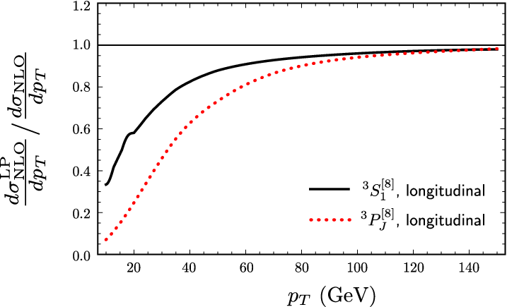
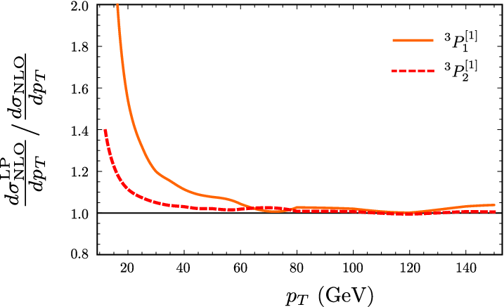
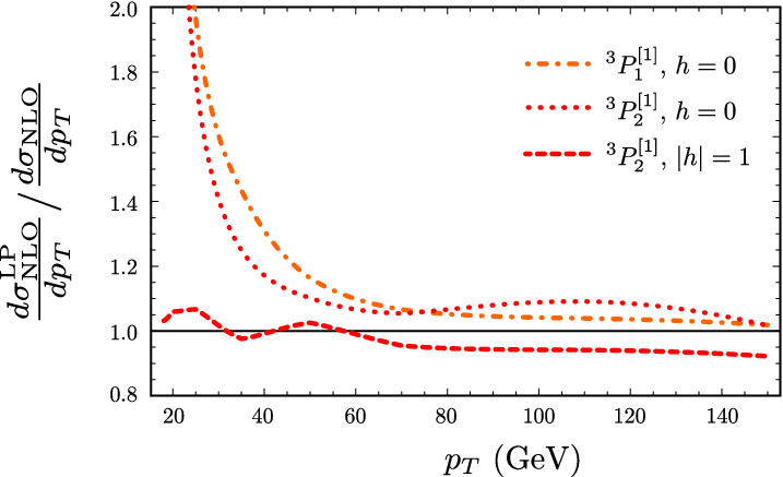
We first compare our results for $d\sigma^{\rm LP}_{\rm NLO}/dp_{T}$ with $d\sigma_{\rm NLO}/dp_{T}$, the fixed-order SDC accurate through NLO. Figures 1–4 show the ratios $(d\sigma^{\rm LP}_{\rm NLO}/dp_{T})/(d\sigma_{\rm NLO}/dp_{T})$ for the polarized and unpolarized final states in the process $pp\to H+X$ at $\sqrt{s}=7$ TeV and $|y|<1.2$.

In Fig. 1, we show the ratios $(d\sigma^{\rm LP}_{\rm NLO}/dp_{T})/(d\sigma_{\rm NLO}/dp_{T})$ for unpolarized final states in the ${}^{3}S_{1}^{[8]},{}^{1}S_{0}^{[8]}$, and ${}^{3}P_{J}^{[8]}$ channels. As $p_{T}$ increases, the ratios for the ${}^{3}S_{1}^{[8]}$ and ${}^{3}P_{J}^{[8]}$ channels quickly approach unity because the LP-fragmentation contribution dominates the SDCs. This approach to unity is slower for the ${}^{1}S_{0}^{[8]}$ channel because the FF for the ${}^{1}S_{0}^{[8]}$ channel does not receive enhancements near $z=1$ from a Dirac $\delta$ function or plus distributions that are the remnants of soft divergences that cancel between real and virtual gluon-emission processes.²² 2 It was shown in Ref. [46] that the ratio $(d\sigma^{\rm LP}_{\rm NLO}/dp_{T}+d\sigma^{\rm NLP}_{\rm NLO}/dp_{T})/(d\sigma_{\rm NLO}/dp_{T})$, which takes into account both the LP and NLP contributions, approaches unity much faster for the ${}^{1}S_{0}^{[8]}$ channel than does the ratio $(d\sigma^{\rm LP}_{\rm NLO}/dp_{T})/(d\sigma_{\rm NLO}/dp_{T})$. At small $p_{T}$, the ratio $(d\sigma^{\rm LP}_{\rm NLO}/dp_{T})/(d\sigma_{\rm NLO}/dp_{T})$ is larger for the ${}^{3}P_{J}^{[8]}$ channel than for the ${}^{3}S_{1}^{[8]}$ and ${}^{1}S_{0}^{[8]}$ channels because, for the ${}^{3}P_{J}^{[8]}$ channel, the LO and NLO contributions in the denominator tend to cancel.

In Fig. 2, we show the ratios $(d\sigma^{\rm LP}_{\rm NLO}/dp_{T})/(d\sigma_{\rm NLO}/dp_{T})$ for longitudinal final states in the ${}^{3}S_{1}^{[8]}$ and ${}^{3}P_{J}^{[8]}$ channels. The approach of each of these ratios to unity is slow. As was the case for the ratio of cross sections in the ${}^{1}S_{0}^{[8]}$ channel, the slow approach to unity is a consequence of the fact that the FFs are not enhanced near $z=1$ by a Dirac $\delta$ function or plus distributions.

In Fig. 3, we show the ratios $(d\sigma^{\rm LP}_{\rm NLO}/dp_{T})/(d\sigma_{\rm NLO}/dp_{T})$ for unpolarized final states in the color-singlet $P$-wave channels. We show the ratios for the polarized final states in Fig. 4. Here, $h$ is the helicity of the $Q\bar{Q}$ pair in the final state. The behaviors are similar to those for the ${}^{3}P_{J}^{[8]}$ channel, except for the case of $J=2$ with $|h|=1$, for which the ratio $(d\sigma^{\rm LP}_{\rm NLO}/dp_{T})/(d\sigma_{\rm NLO}/dp_{T})$ is almost constant. We note that the deviation of $(d\sigma^{\rm LP}_{\rm NLO}/dp_{T})/(d\sigma_{\rm NLO}/dp_{T})$ from unity at large $p_{T}$ is of the same relative size as the statistical uncertainty in the NLO calculation.

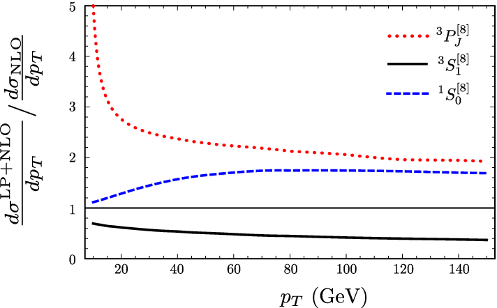
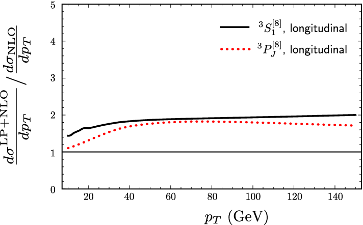
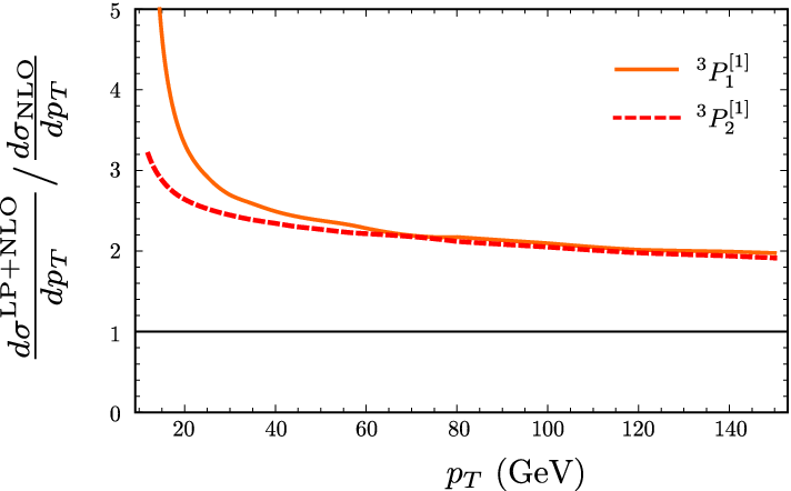
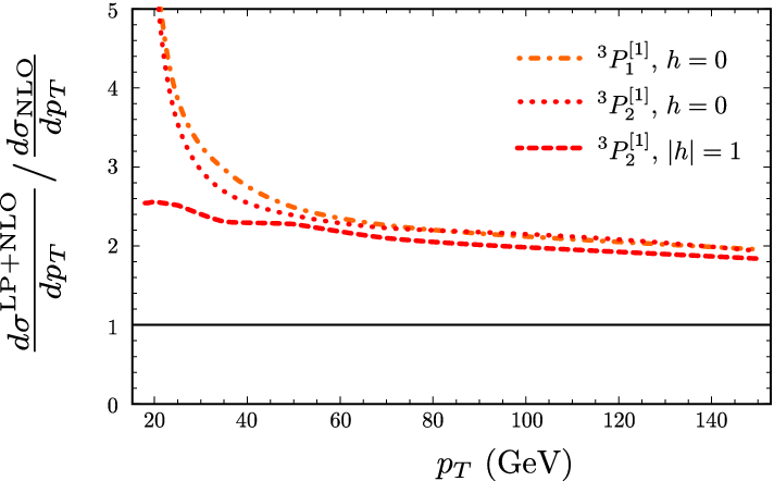
Next we compare $d\sigma^{\rm LP+NLO}_{\rm NLO}/dp_{T}$, the SDC that includes both the fixed-order corrections through NLO and the additional LP corrections, with $d\sigma_{\rm NLO}/dp_{T}$, the SDC that includes fixed-order corrections through NLO. Specifically, we show the ratios $(d\sigma^{\rm LP+NLO}_{\rm NLO}/dp_{T})/(d\sigma_{\rm NLO}/dp_{T})$ for the polarized and unpolarized final states in Figs. 5–8. With the exception of the ${}^{3}S_{1}^{[8]}$ channel, the additional LP-fragmentation contributions are of the order of $100\%$ at large $p_{T}$. As we have mentioned, because there is a partial cancellation between the LO and the NLO contributions in the ${}^{3}P_{J}^{[8]}$ channel, the additional LP fragmentation corrections have a significant impact on the shape in that channel. For the ${}^{3}S_{1}^{[8]}$ channel the additional LP-fragmentation contributions are negative and only mildly alter the shape.

As was pointed out in Ref. [25], the effects from the all-orders resummation of logarithms of $p_{T}^{2}/m_{c}^{2}$ are small. In the case of the ${}^{3}S_{1}^{[8]}$ channel, almost all of the effects of the large logarithms are already accounted for in the NLO contribution. In the cases of the ${}^{1}S_{0}^{[8]}$ and ${}^{3}P_{J}^{[8]}$ channels, the all-orders resummations of logarithms shift the FFs by only about $2\%$ and $5\%$, respectively, at $p_{T}=52.7$ GeV because contributions from the running of $\alpha_{s}$ and from the DGLAP splitting cancel. Hence, almost all of the large additional LP corrections that we find arise from nonlogarithmic contributions of order $\alpha_{s}^{5}$.

Finally, we discuss the LP-fragmentation contribution to the ${}^{3}S_{1}^{[1]}$ channel. Since the FF for this channel begins at order $\alpha_{s}^{3}$, the ${}^{3}S_{1}^{[1]}$ channel receives an LP contribution that begins at order $\alpha_{s}^{5}$ (NNLO). We do not include this LP-fragmentation contribution in our analysis. However, we have estimated its size by making use of the FF at order $\alpha_{s}^{3}$. At $p_{T}=10$ GeV, the LP contribution is about an order of magnitude smaller than the fixed-order contribution through NLO. The LP contribution reaches the same size as the fixed-order contribution through NLO at around $p_{T}=50$ GeV. Finally, when $p_{T}=130$ GeV, the LP contribution is almost an order of magnitude larger than the fixed-order contribution through NLO. Although the LP-fragmentation contribution can have a significant effect on the color-singlet contribution at large $p_{T}$, its effect on the cross section is only of the order of $1\%$ of the measured cross section at $p_{T}=130$ GeV.

In this section we extract the color-octet LDMEs by fitting the cross-section predictions that are based on the LP$+$NLO SDCs to the measured cross sections. We use the resulting LDMEs to make predictions for the prompt-$J/\psi$ polarization. In order to suppress possible nonfactorizing contributions, we fit only to data for which $p_{T}$ is greater than $3m_{H}$, where $m_{H}$ is the quarkonium mass. Since the shape of the $p_{T}$ distribution determines the LDMEs, it is crucial to use the data at the highest $p_{T}$ values in the fits.

In the case of the direct $J/\psi$ cross section, we estimate the theoretical uncertainties in the SDCs to be $25\%$ of the central values. We arrived at these uncertainties by varying the factorization scale $\mu_{f}$ and the renormalization scale $\mu_{r}$ independently between $\frac{1}{2}m_{T}$ and $2m_{T}$. This $25\%$ uncertainty is also roughly the size of the uncertainty that one would expect from uncalculated corrections of higher order in $v$. In the cases of the cross sections of the excited charmonium states, we take the uncertainties to be $30\%$ of the central values because the $v^{2}$ for those states is larger than for the $J/\psi$.

References

- [1] Y.-Q. Ma, K. Wang, and K.-T. Chao, Phys. Rev. D 84, 114001 (2011) [arXiv:1012.1030 [hep-ph]].
- [2] M. Butenschoen and B. A. Kniehl, Phys. Rev. Lett. 106, 022003 (2011) [arXiv:1009.5662 [hep-ph]].
- [3] Y.-Q. Ma, K. Wang, and K.-T. Chao, Phys. Rev. Lett. 106, 042002 (2011) [arXiv:1009.3655 [hep-ph]].
- [4] K.-T. Chao, Y.-Q. Ma, H.-S. Shao, K. Wang, and Y.-J. Zhang, Phys. Rev. Lett. 108, 242004 (2012) [arXiv:1201.2675 [hep-ph]].
- [5] M. Butenschoen and B. A. Kniehl, Phys. Rev. Lett. 108, 172002 (2012) [arXiv:1201.1872 [hep-ph]].
- [6] B. Gong, L.-P. Wan, J.-X. Wang, and H.-F. Zhang, Phys. Rev. Lett. 110, 042002 (2013) [arXiv:1205.6682 [hep-ph]].
- [7] M. Butenschoen and B. A. Kniehl, Phys. Rev. D 84, 051501 (2011) [arXiv:1105.0820 [hep-ph]].
- [8] M. Butenschoen and B. A. Kniehl, Phys. Rev. Lett. 104, 072001 (2010) [arXiv:0909.2798 [hep-ph]].
- [9] M. Butenschoen and B. A. Kniehl, Phys. Rev. Lett. 107, 232001 (2011) [arXiv:1109.1476 [hep-ph]].
- [10] G. T. Bodwin, E. Braaten, and G. P. Lepage, Phys. Rev. D 51, 1125 (1995); 55, 5853(E) (1997) [hep-ph/9407339].
- [11] D. Acosta et al. [CDF Collaboration], Phys. Rev. D 71, 032001 (2005) [hep-ex/0412071].
- [12] S. Chatrchyan et al. [CMS Collaboration], JHEP 1202, 011 (2012) [arXiv:1111.1557 [hep-ex]].
- [13] T. Affolder et al. [CDF Collaboration], Phys. Rev. Lett. 85, 2886 (2000) [hep-ex/0004027].
- [14] A. Abulencia et al. [CDF Collaboration], Phys. Rev. Lett. 99, 132001 (2007) [arXiv:0704.0638 [hep-ex]].
- [15] S. Chatrchyan et al. [CMS Collaboration], Phys. Lett. B 727, 381 (2013) [arXiv:1307.6070 [hep-ex]].
- [16] C. Adloff et al. [H1 Collaboration], Eur. Phys. J. C 25, 25 (2002) [hep-ex/0205064].
- [17] F. D. Aaron et al. [H1 Collaboration], Eur. Phys. J. C 68, 401 (2010) [arXiv:1002.0234 [hep-ex]].
- [18] M. Butenschoen and B. A. Kniehl, Mod. Phys. Lett. A 28, 1350027 (2013) [arXiv:1212.2037 [hep-ph]].
- [19] M. Butenschoen, Z.-G. He, and B. A. Kniehl, Phys. Rev. Lett. 114, 092004 (2015) [arXiv:1411.5287 [hep-ph]].
- [20] R. Aaij et al. [LHCb Collaboration], Eur. Phys. J. C 75, 311 (2015) [arXiv:1409.3612 [hep-ex]].
- [21] H. Han, Y.-Q. Ma, C. Meng, H.-S. Shao, and K.-T. Chao, Phys. Rev. Lett. 114, 092005 (2015) [arXiv:1411.7350 [hep-ph]].
- [22] H.-F. Zhang, Z. Sun, W.-L. Sang and R. Li, Phys. Rev. Lett. 114, no. 9, 092006 (2015) [arXiv:1412.0508 [hep-ph]].
- [23] J. C. Collins and D. E. Soper, Nucl. Phys. B 194, 445 (1982).
- [24] Z.-B. Kang, J.-W. Qiu, and G. Sterman, Phys. Rev. Lett. 108, 102002 (2012) [arXiv:1109.1520 [hep-ph]].
- [25] G. T. Bodwin, H. S. Chung, U-R. Kim, and J. Lee, Phys. Rev. Lett. 113, 022001 (2014) [arXiv:1403.3612 [hep-ph]].
- [26] V. N. Gribov and L. N. Lipatov, Sov. J. Nucl. Phys. 15, 438 (1972) [Yad. Fiz. 15, 781 (1972)].
- [27] L. N. Lipatov, Sov. J. Nucl. Phys. 20, 94 (1975) [Yad. Fiz. 20, 181 (1974)].
- [28] Y. L. Dokshitzer, Sov. Phys. JETP 46, 641 (1977) [Zh. Eksp. Teor. Fiz. 73, 1216 (1977)].
- [29] G. Altarelli and G. Parisi, Nucl. Phys. B 126, 298 (1977).
- [30] F. Aversa, P. Chiappetta, M. Greco, and J. P. Guillet, Nucl. Phys. B 327, 105 (1989).
- [31] B. Jager, A. Schafer, M. Stratmann, and W. Vogelsang, Phys. Rev. D 67, 054005 (2003) [hep-ph/0211007].
- [32] Y.-Q. Ma, J.-W. Qiu, and H. Zhang, Phys. Rev. D 89, 094029 (2014) [arXiv:1311.7078 [hep-ph]].
- [33] Y.-Q. Ma, J.-W. Qiu, and H. Zhang, JHEP 1506, 021 (2015) [arXiv:1501.04556 [hep-ph]].
- [34] E. Braaten and T. C. Yuan, Phys. Rev. D 50, 3176 (1994) [hep-ph/9403401, hep-ph/9403401].
- [35] E. Braaten and J. Lee, Nucl. Phys. B 586, 427 (2000) [hep-ph/0004228].
- [36] E. Braaten and Y.-Q. Chen, Phys. Rev. D 55, 2693 (1997) [hep-ph/9610401].
- [37] G. T. Bodwin, U-R. Kim, and J. Lee, JHEP 1211, 020 (2012) [arXiv:1208.5301 [hep-ph]].
- [38] P. Cho, M. B. Wise, and S. P. Trivedi, Phys. Rev. D 51, 2039 (1995) [hep-ph/9408352].
- [39] G. T. Bodwin, H. S. Chung, U-R. Kim, and J. Lee, Phys. Rev. D 91, no. 7, 074013 (2015) [arXiv:1412.7106 [hep-ph]].
- [40] J. P. Ma, Phys. Rev. D 53, 1185 (1996) [hep-ph/9504263].
- [41]
H. Zhang, “QCD factorization for heavy quarkonium production
and fragmentation functions,” A Dissertation for the Degree of Doctor
of Philosophy in Physics, Stony Brook University, August, 2014
(http://graduate.physics.sunysb.edu/announ/theses/zhang-hong-august-2014.pdf). - [42] T. C. Yuan, Phys. Rev. D 50, 5664 (1994) [hep-ph/9405348].
- [43] E. Braaten, K. Cheung, and T. C. Yuan, Phys. Rev. D 48, 4230 (1993) [hep-ph/9302307].
- [44] E. Braaten and T. C. Yuan, Phys. Rev. Lett. 71, 1673 (1993) [hep-ph/9303205].
- [45] E. Braaten and T. C. Yuan, Phys. Rev. D 52, 6627 (1995) [hep-ph/9507398].
- [46] Y.-Q. Ma, J.-W. Qiu, G. Sterman, and H. Zhang, Phys. Rev. Lett. 113, 142002 (2014) [arXiv:1407.0383 [hep-ph]].
- [47] T. Aaltonen et al. [CDF Collaboration], Phys. Rev. D 80, 031103 (2009) [arXiv:0905.1982 [hep-ex]].
- [48] V. Khachatryan et al. [CMS Collaboration], Phys. Rev. Lett. 114, 191802 (2015) [arXiv:1502.04155 [hep-ex]].
- [49] E. J. Eichten and C. Quigg, Phys. Rev. D 52, 1726 (1995) [hep-ph/9503356].
- [50] P. Faccioli, V. Knünz, C. Lourenço, J. Seixas, and H. K. Wöhri, Phys. Lett. B 736, 98 (2014) [arXiv:1403.3970 [hep-ph]].
- [51] G. Aad et al. [ATLAS Collaboration], JHEP 1407, 154 (2014) [arXiv:1404.7035 [hep-ex]].
- [52] H. S. Chung, J. Lee, and C. Yu, Phys. Rev. D 78, 074022 (2008) [arXiv:0808.1625 [hep-ph]].
- [53] P. Faccioli, C. Lourenço, J. Seixas, and H. K. Wöhri, Phys. Rev. D 83, 096001 (2011) [arXiv:1103.4882 [hep-ph]].
- [54] M. Artuso et al. [CLEO Collaboration], Phys. Rev. D 80, 112003 (2009) [arXiv:0910.0046 [hep-ex]].
- [55] G. T. Bodwin, H. S. Chung, D. Kang, J. Lee, and C. Yu, Phys. Rev. D 77, 094017 (2008) [arXiv:0710.0994 [hep-ph]].
- [56] R. Aaij et al. [LHCb Collaboration], Phys. Lett. B 718, 431 (2012) [arXiv:1204.1462 [hep-ex]].
- [57] Y.-Q. Ma, K. Wang, and K.-T. Chao, Phys. Rev. D 83, 111503 (2011) [arXiv:1002.3987 [hep-ph]].
- [58] D. Li, Y.-Q. Ma, and K.-T. Chao, Phys. Rev. D 83, 114037 (2011) [arXiv:1106.4262 [hep-ph]].
- [59] H.-S. Shao, Y.-Q. Ma, K. Wang, and K.-T. Chao, Phys. Rev. Lett. 112, 182003 (2014) [arXiv:1402.2913 [hep-ph]].
- [60] L. Jia, L. Yu, and H.-F. Zhang, arXiv:1410.4032 [hep-ph].
- [61] H.-S. Shao, H. Han, Y.-Q. Ma, C. Meng, Y.-J. Zhang, and K.-T. Chao, JHEP 1505, 103 (2015) [arXiv:1411.3300 [hep-ph]].
- [62] G. T. Bodwin, H. S. Chung, U-R. Kim, and J. Lee, arXiv:1504.06019 [hep-ph].