Interpreting the Global 21-cm Signal from High Redshifts.
II. Parameter Estimation for Models of Galaxy Formation
Abstract
Following our previous work, which related generic features in the sky-averaged (global) 21-cm signal to properties of the intergalactic medium, we now investigate the prospects for constraining a simple galaxy formation model with current and near-future experiments. Markov-Chain Monte Carlo fits to our synthetic dataset, which includes a realistic galactic foreground, a plausible model for the signal, and noise consistent with 100 hours of integration by an ideal instrument, suggest that a simple four-parameter model that links the production rate of Lyman-, Lyman-continuum, and X-ray photons to the growth rate of dark matter halos can be well-constrained (to dex in each dimension) so long as all three spectral features expected to occur between are detected. Several important conclusions follow naturally from this basic numerical result, namely that measurements of the global 21-cm signal can in principle (i) identify the characteristic halo mass threshold for star formation at all redshifts , (ii) extend upper limits on the normalization of the X-ray luminosity star-formation rate (-SFR) relation out to , and (iii) provide joint constraints on stellar spectra and the escape fraction of ionizing radiation at . Though our approach is general, the importance of a broad-band measurement renders our findings most relevant to the proposed Dark Ages Radio Explorer, which will have a clean view of the global 21-cm signal from MHz from its vantage point above the radio-quiet, ionosphere-free lunar far-side.
Subject headings
early universe — diffuse radiation – epoch of reionizationI. Introduction
The high redshift () Universe has become a frontier in recent years, as it was the time in which stars, galaxies, and black holes first formed, bringing an end to the cosmic “dark ages” and initiating the “cosmic dawn.” Preliminary searches for these objects have commenced, primarily with the Hubble Space Telescope, and have begun to find very bright galaxies at [80, 15, 50]. However, it is the individually faint but overwhelmingly numerous galaxies that likely usher in the Epoch of Reionization (EoR), and may account for a substantial fraction of the ionizing photons required to bring the EoR to a close by [72, 76, e.g.,]. If the galaxy luminosity function flattens considerably at the low-luminosity end [52] or the formation efficiency of massive Population III stars is low, even the James Webb Space Telescope may struggle to find faint galaxies beyond [78]. Measurements of the cosmic microwave background (CMB), in conjunction with independent constraints on the ionization and star-formation histories, support a relatively short EoR, and thus a relatively modest galaxy population at [10, 64, 7].
Observations at low radio frequencies – corresponding to highly redshifted 21-cm “spin-flip” radiation from neutral hydrogen atoms – are a promising complement to CMB measurements and optical and near-infrared imaging campaigns to constrain the high redshift galaxy population [40, 65, 22]. Numerous efforts to detect the 21-cm background are already underway, including both its spatial fluctuations and monopole spectral signature. For instance, observations with the Precision Array for Probing the Epoch of Reionization indicate an X-ray heated IGM at [54, 1, 57], while the Experiment to Detect the Global EoR Signal (EDGES) is so far the only 21-cm experiment to set lower limits on the duration of the reionization epoch [8, ;].
Targeting the sky-averaged (“global”) 21-cm spectrum may enable more rapid progress at the highest redshifts (), as it can in principle be detected with a single well-calibrated dipole receiver. Several ground-based experiments are underway [8, 75, 28, 69, e.g.; EDGES, SCI-HI, LEDA, BIGHORNS;], though space-based observatories will be required to probe the cosmic dawn at [9, e.g., the Dark Ages Radio Explorer, (DARE);], as the Earth’s ionosphere reflects and refracts radio signals at low frequencies [74, 11]. Interferometers are in principle capable of measuring the global 21-cm signal, so long as they are compact [61, 68] or can overcome challenges in lunar occultation techniques [73].
No matter the observing technique, all global experiments must cope with the Galactic foreground, which is times brighter than the cosmological signal in temperature. Though strong and spatially variable, the Galactic foreground is spectrally smooth [12], in contrast to the expected high redshift signal which is spatially invariant but spectrally complex. It is this spectral structure that should enable one to distinguish foreground from signal [65, 26, 20, 63], especially if one observes multiple (semi-) independent sky regions [34, 39, 70]. Though current constraints do not rule out unresolved spectral structure at the level of the high redshift signal, theoretical arguments favor a smooth foreground at the relevant frequencies [56, 6]. Extragalactic point sources are another foreground, but for experiments with broad beams, their combined contribution averages into another diffuse spectrally smooth foreground [65].
Given that the global 21-cm signal is an indirect probe of high- galaxies, some modeling is required to convert observational quantities to constraints on the properties of the Universe’s first galaxies. Though numerous studies have performed forward modeling to predict the strength of the global 21-cm signal [20, 63], few have attempted to infer physical parameters of interest from synthetic datasets. Such forecasting exercises are incredibly useful tools for designing instruments and planning observing strategies, as they illuminate the mapping between constraints on observable quantities and model parameters of interest. Both Fisher matrix and Markov Chain Monte Carlo (MCMC) approaches have been employed by the power spectrum community [58, 29, e.g.,], the latter providing a powerful generalization that does not require the assumption of Gaussian errors or perfect recovery of the maximum likelihood point.
Most work to date has instead focused on forecasting constraints on phenomenological parameters of interest, e.g., the timing and duration of reionization [39], the depth and width of the deep minimum expected near MHz prior to reionization [6], or all three spectral features predicted to occur between [63, 34]. These spectral “turning points” in the global 21-cm spectrum provide a natural basis for parameter forecasting, as they persist over large ranges of parameter space [63], can be extracted from the foreground with realistic instruments and integration times [34, 61, 6, at least under the assumption of a negligible ionosphere;], and can be extracted from the foreground even when their positions are not used as the parameters of a signal model [33]. They can also be interpreted fairly robustly in terms of the physical properties of the IGM, at least in simple two-phase models [45, hereafter Paper I]. Given the viability of the turning points as “products” of global 21-cm signal extraction pipelines, we will use them as a launching point in this paper from which to explore the prospects for constraining astrophysical parameters of interest with observations of the global 21-cm signal. Importantly, we will consider all three turning points simultaneously, rendering our findings particularly applicable to DARE, whose band extends from in order to maximize the likelihood of detecting all three features at once.
This paper is organized as follows. In Section 2 we outline our methods for modeling the global 21-cm signal and parameter estimation. Section 3 contains our main results, with a discussion to follow in Section 4. In Section 5, we summarize our results. We use the most up-to-date cosmological parameters from Planck throughout [10, last column in Table 4 of].
II. NUMERICAL METHODS
In order to forecast constraints on the properties of the first galaxies, we will need (1) a model for the global 21-cm signal, (2) estimates for the precision with which this signal can be extracted from the foregrounds, and (3) an algorithm capable of efficiently exploring a multi-dimensional parameter space to find the best-fit model parameters and their uncertainties. The next three sub-sections are devoted to describing these three pieces of our pipeline in turn.
II.1. Physical Model for the Global 21-cm Signal
Our approach to modeling the global 21-cm signal is similar to that presented in several other published works [2, 20, 63, 44, e.g.,], so we will only discuss it here briefly. The primary assumption of our model is that the radiation backgrounds probed by the turning points are generated by stars and their byproducts, which form at a rate proportional to the rate of baryonic collapse into dark matter haloes. That is, we model the star-formation rate density (SFRD) as
| (1) |
where is the fraction of matter in collapsed halos with virial temperatures greater than , is the mean baryon density today, and is the star formation efficiency. We use a fixed rather than a fixed because it provides physical insight into the processes governing star-formation, as one can easily identify the atomic and molecular cooling thresholds of and K. Note that a fixed value of results in a time-dependent mass threshold, .
In order to generate a model realization of the global 21-cm signal, we must convert star-formation to photon production. Given that the three spectral turning points probe the history of ionization, heating, and emission, we will split the production of radiation into three separate bands: (1) from the resonance to the Lyman-limit, , which we refer to as the Lyman-Werner (LW) band despite its inclusion of photons below eV, (2) hydrogen-ionizing photons, with energies , and (3) X-rays, with energies exceeding 0.1 keV. Each radiation background is linked to the SFRD through a scaling parameter , which converts a rate of star formation to a rate of photon (or energy) production). The background intensity is then given by
| (2) |
where , and the ionization rate by
| (3) |
The rate of X-ray heating is defined instead in terms of an energy per unit star-formation, i.e.,
| (4) |
where is the normalization of the -SFR relation, which we take to be following Furlanetto [20]11 1 Furlanetto [20] computed this value by extrapolating the 2-10 keV -SFR relation of Grimm et al. [30] above 0.2 keV, assuming an unabsorbed power-law spectrum. Our reference value of (which is dimensionless, unlike and ) is chosen to match recent analyses in the 0.5-8 keV band, which find [41]. Note that we have absorbed into the parameters, i.e.
| (5) | ||||
| (6) | ||||
| (7) |
where and are the number of LW and ionizing photons emitted per stellar baryon, is the escape fraction of ionizing radiation, and scales the -SFR relation.
Given , , and the background intensity, , we can evolve the ionization and thermal state of intergalactic gas in time, and compute the sky-averaged 21-cm signal, i.e., the differential brightness temperature of HI relative to the CMB, via [20, e.g.,]22 2 Though this expression does not explicitly depend on the density of hydrogen gas (it assumes gas is at the cosmic mean density, ), the global 21-cm signal may still be sensitive to the density provided that fluctuations in the ionization and/or spin temperature of HI gas are correlated with its density.
| (8) |
where is the CMB temperature, is the volume-averaged ionization fraction,
| (9) |
with representing the volume-filling factor of HII regions and the ionized fraction in the bulk IGM. is the excitation or “spin” temperature of neutral hydrogen, which quantifies the number of hydrogen atoms in the hyperfine triplet and singlet states,
| (10) |
where is the gas kinetic temperature, [17], and and the ’s take on their usual cosmological meaning. We compute the collisional coupling coefficient, , by interpolating between the tabulated values in Zygelman [81] with a cubic spline, and take . We perform these calculations using the Accelerated Reionization Era Simulations (ares) code33 3 https://bitbucket.org/mirochaj/ares;v0.1, which is the union of a 1-D radiative transfer code developed in Mirocha et al. [46] and uniform radiation background code described in Mirocha [44]. See §2 of Mirocha [44] for a more detailed description of the global 21-cm signal modeling procedure.

| Quantity | Reference Value | EM1 | EM2 | Description |
|---|---|---|---|---|
| 47.4 | Onset of coupling | |||
| 71.0 | Onset of heating | |||
| 111.4 | Beginning of reionization | |||
| -4.4 | n/a | n/a | Depth when coupling begins | |
| -124.8 | Depth of absorption trough | |||
| 19.2 | Height of emission feature | |||
| 9.25 | n/a | n/a | Midpoint of reionization | |
| 0.066 | n/a | n/a | CMB optical depth |
Note. — Observational properties of our reference model (solid black lines in Figure 1), and the best-fit and uncertainties for each extraction model (EM) we consider. Subscripts indicate different turning points, i.e., the cosmic dawn feature when the Wouthuysen-Field effect first drives to (B), the absorption trough, which indicates the onset of heating (C), and the beginning of reionization (D). EM1 and EM2 differ in the number of independent sky regions assumed (1 vs. 2), and in the complexity of the foreground model (3rd vs. 4th order polynomial), which leads primarily to a more robust detection of turning point D for EM2. All errors are , and correspond directly to the diagonal elements of the turning point covariance matrix.
Figure 1 shows our reference model (properties of which are listed in Table 1), and the modulations in its structure that occur when varying , , , and . It is immediately clear that affects the locations of all three turning points, whereas each parameter affects at most two. We should therefore expect that in principle, an observation containing all three features will have the best chance to constrain , though this will be complicated at the lowest redshifts where becomes a weaker function of (see bottom panel of Figure 2).
Figure 1 also shows that will be difficult to constrain using global signal data at these frequencies, as even factor of 10 changes lead only to small changes in the signal (at MHz), whereas factor of 10 changes in and are mK effects. There are also clear degeneracies between and the parameters. Exploring those degeneracies and determining the prospects for constraining each parameter independently are our primary goals in this work. The results will in large part depend on how accurately the signal can be recovered from the foregrounds, which we discuss in the next subsection.
Before moving on to signal recovery, it is worth reiterating that our approach cannot be used to constrain the normalization of the SFRD, since we have absorbed the star-formation efficiency into the parameters. However, we can constrain the rate-of-change in the SFRD, as it is uniquely determined by . It is illustrative to quantify this using an effective power-law index
| (11) |
which enables a straightforward comparison with empirical models, which are often power-laws, i.e., , in which case . The values of our model are independent of so long as , and generally fall within the (broad) range of values permitted by observations of high- galaxies [50, 64], as shown in the top panel of Figure 2.

II.2. Signal Extraction
In order to fit a physical model to the turning points of the global 21-cm signal, we require best-fit values for the turning point positions and estimates for uncertainties. To do this, we build on the work of Harker et al. [34] and Harker et al. [33], who introduced a MCMC technique for fitting global 21-cm signal data. The basic approach is to simultaneously fit a model for the galactic foreground, the global 21-cm signal, and in general, parameters of the instrument (e.g., its response as a function of frequency), assuming some amount of integration time, , and the number of independent sky regions observed, . The foreground is modeled as a polynomial in space, while the astrophysical signal is modeled as either a spline [34] or series of functions,
| (12) |
that represent , , and [33]. The free parameters of the tanh model are the “step height,” , pivot redshift, , and a duration, .
The tanh approach to modeling the global 21-cm signal was chosen for numerous reasons. First and foremost, it was chosen as a computationally efficient substitute for more expensive, but physically-motivated models like those investigated in this paper. Some alternative intermediaries include the ‘turning points’ parameterization [63, 34] or models that treat the absorption feature as a Gaussian [6]. Both are comparably cheap computationally, but cannot capture the detailed shape of physical models. Perhaps most importantly, the spline and Gaussian models are purely phenomenological, making them difficult to interpret in terms of IGM or galaxy properties and thus incapable of incorporating independent prior information on e.g., the ionization or thermal history. The approach, on the other hand, can mimic the shape of typical global 21-cm signal models extremely well, and can be immediately related to physical properties of the IGM.
Harker et al. [33] presented a suite of calculations spanning the 2-D parameter space defined by and . In the calculations, confidence contours of the turning point positions narrowed enough to reveal subtle biases in their recovered positions, which led to biases in constraints on physical properties of the IGM as well. These shifts were interpreted to be due to degeneracies between the signal and the foreground at high frequencies, as they could be mitigated by using a more sophisticated foreground model or, at the expense of losing information from turning point D, simply by truncating the bandpass at 100 MHz. However, even with unbiased constraints on the turning point positions, biases in the IGM properties persisted, likely because the is not a perfect match in shape to the physical model injected into the synthetic dataset. Though we suspect that biases in constraints on the turning points are a persistent feature in datasets employing the tanh, turning point constraints from the hr cases in [33] are broad enough to hide such biases. In using the hr results, we should then expect to be able to obtain unbiased constraints on the parameters of our physical model in the present work. We also only analyze cases using one and two sky regions, for which model selection will be more immediately tractable computationally [32].
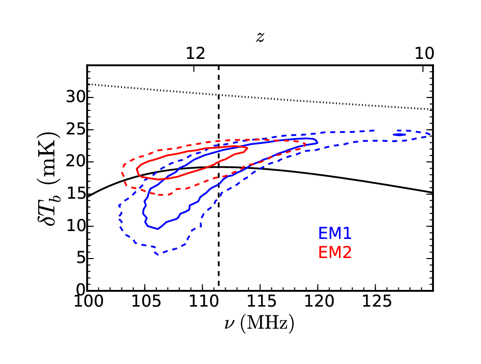
Now, back to the simplest model of Harker et al. [33] (EM1 in Table 1). This calculation assumed a single sky region, 100 hours of integration, and a third-order polynomial for the galactic foreground44 4 It seems likely that in practice a higher order polynomial will be needed to fit out instrumental effects [6, e.g.,]. However, here our synthetic datasets contain foregrounds with no structure beyond a polynomial of order three (or four), meaning third and fourth order polynomials can fit the foreground perfectly (by construction).. Harker et al. [33] investigated the generic case of an idealized instrument (a flat 85% response function), though this could easily be modified to enable forecasting for non-ideal instruments. The foreground and astrophysical signal were simultaneously fit using the parallel-tempering sampler in the publicly available emcee code55 5 http://dan.iel.fm/emcee/current/ [18], a python implementation of the affine-invariant MCMC sampler of Goodman & Weare [27], from which constraints on the positions of the turning points followed straightforwardly. The errors on the turning points are in general not Gaussian, and are often correlated with one another, though for the purposes of our fitting, we approximate the errors as 1-D independent Gaussians since covariances are likely to depend on the choice of signal parameterization. In addition to EM1, we also investigate the results of a fit using a 4th order log-polynomial for the foreground model, which we refer to as EM2. Table 1 summarizes the different signal extraction models, while Figure 3 illustrates the primary difference between the two extraction models graphically.
II.3. Parameter Estimation
With a physical model for the global 21-cm signal (§II.1) and a set of constraints on the turning point positions (§II.2), we then explore the posterior probability distribution function (PDF) for the model parameters, , given the data, . That is, we evaluate Bayes’ theorem,
| (13) |
The log-likelihood is given by
| (14) |
where is the “measurement” with errors (i.e., the values listed in columns 3 and 4 of Table 1), and represents a vector of turning point positions extracted from the model global 21-cm signal generated with parameters . This “two-stage approach” to fitting the global 21-cm signal – the first stage having been conducted by Harker et al. [33] – is much more tractable computationally than a direct “one-stage” fit to a mock dataset using a physical model. Note that the brightness temperature of turning point B, , is tightly coupled to its frequency, so we are effectively only using 5 independent data points in our fits.
| Parameter | Description | Input | Min | Max |
|---|---|---|---|---|
| Min. virial temp. of star-forming haloes | ||||
| Ly- efficiency | 969 | |||
| X-ray efficiency | 0.02 | |||
| Ionizing efficiency | 40 |
Note. — Parameter space explored for results presented in §III. The first two columns indicate the parameter name and a brief description, the third column is the “true value” of the parameter in our reference model, while the last two columns indicate the bounds of the priors for each parameter, all of which are assumed to be uninformative, i.e., modeled as uniform distributions between the minimum and maximum allowed values.
To explore this four-dimensional space, we use emcee. We assume broad, uninformative priors on all parameters (listed in Table 2), but note that our physical model implicitly imposes three additional constraints on the astrophysical signal:
- 1.
We neglect exotic heat sources at high-, which confines turning point B to a narrow “track” at MHz.
- 2.
We assume that the Universe cannot cool faster than the Hubble expansion, which sets a redshift-dependent lower limit on the strength of the absorption signal (lower dotted curve in all panels of Figure 1).
- 3.
We assume the mean density of the IGM we observe is the universal mean density, i.e., it has , which prevents the signal from exceeding the “saturated limit,” in which and (upper dotted curve in all panels of Figure 1).
Our code could be generalized to accommodate exotic heating models, though this is beyond the scope of this paper. Bullets 2 and 3 above are manifestly true for gas at the cosmic mean density (via Equation 8), though imaging campaigns will likely see patches of IGM whose brightness temperatures exceed (in absolute value) these limits, owing to over-densities .
For all calculations presented in this work, we use 384 walkers, each of which take a 150 step burn-in, at which point they are re-initialized in a tight ball centered on the region of highest likelihood identified during the burn-in. We then run for 150 steps more (per walker), resulting in MCMC chains with 57,600 links. The mean acceptance fraction, i.e., the number of proposed steps that are actually taken during our MCMC runs, is . The runs are well-converged, as we see no qualitative differences in the posterior distributions when we compare the last two 10,000 element subsets of the full chain.
III. Results
Each MCMC fit yields 57,600 samples of the posterior distribution, which is a 4-dimensional distribution in space. However, we also analyze each realization of the global 21-cm signal on-the-fly as the MCMC runs, saving IGM quantities of interest every between , as well as at the turning points. To build upon the analytical arguments presented in Paper I, which provided a basis for interpreting the turning points in terms of IGM properties, we start with an analysis of the inferred IGM properties at the turning points in §III.1, deferring a full analysis of the IGM history to future work. Readers interested only in the constraints on our four-parameter model can proceed directly to §III.2.
III.1. Constraints on the Intergalactic Medium
We begin by showing our mock constraints on properties of the IGM at the redshifts of turning points B, C, and D in Figures 4, 5, and 6, respectively66 6 Note that our choice to derive constraints on the IGM parameters at the turning points, rather than at a fixed series of redshifts, is in part responsible for some of the behavior in Figures 5 and 6. This seemed a natural choice given that we fit our model to the turning points alone. Constraints at an arbitrary redshift could be extracted in future studies, for example to compare to independent measurements that do not coincide with the redshifts of the turning points..
Because turning point B primarily probes the background, we focus only on its ability to constrain in Figure 4. The input value is recovered to , with relatively tight error-bars limiting to within a factor of 2. Use of EM2 has little effect on this constraint as its main improvement over EM1 is at frequencies MHz.

Figure 5 shows constraints on the background and thermal history at the redshift of turning point C. In the Myr separating turning points B and C, the background intensity, , has risen by a factor of , though we still constrain its value to within a factor of (panel f). The IGM temperature is limited to , and would otherwise be K at this redshift in the absence of heat sources. There are noticeable degeneracies in the 2-D PDFs, which are not necessarily obvious intuitively.
Let us first focus on the anti-correlations in the - and planes (panels a and d in Figure 5). For this exercise – and those that follow – it will be useful to consider slight excursions away from our reference model. We can see from the lower right panel of Figure 1 that a small increase in will shift turning point B to slightly higher redshifts (lower frequencies) holding all other parameters fixed. Turning point C will also occur earlier than in our reference model (since a stronger background can couple to more rapidly ) and be deeper, since there has been less time for X-rays to heat the IGM, leading to increased contrast between the IGM and the CMB. Panels (a) and (d) in Figure 5 now make sense: the anti-correlations in the - and planes arise because measurement errors permit slight excursions away from the reference model, which if achieved through enhancements to , shift turning points B and C to slightly earlier – and thus cooler – times.
One could also counteract a mild increase in with a corresponding increase in , which enhances heating and thus leads to shallower absorption troughs. However, increasing shifts turning point C to shallower depths and lower frequencies, thus exacerbating the leftward shift caused by larger values of . As a result, would also need to be increased in order to delay the onset of Wouthuysen-Field coupling and heating. Indeed, we will find this series of positive correlations among the physical parameters of our model in the §III.2.
Before moving on to the IGM constraints associated with turning point D, we note that the correlation between and (panel b) is simply because , and is monotonic. Also, apparently the improvement at the highest frequencies offered by EM2 also acts to slightly bias constraints on and relative to their input values. Referring back to Figure 3, we do see a slight bias in the EM2 PDF for turning point D toward larger amplitude, which would require more rapid heating at earlier times. In fact, this is precisely the sense of the bias we see in Figure 5: slightly larger values of at turning point C, and a corresponding downward shift in as described above.

And finally, Figure 6 shows constraints on the ionization and thermal histories at the redshift of turning point D, which occurs at in our input model. The behavior here is complex, as the signal is not yet saturated (i.e., is a poor approximation) and the mean ionized fraction is non-zero (i.e., ). This means the global 21-cm signal depends on both the ionization history and the thermal history, which we may parameterize in terms of the volume filling factor of ionized gas, , the IGM temperature, , and their time-derivatives77 7 Although we use the symbol , we caution that our values should not be compared to extrapolations of constraints on from the forest at . The latter is a probe of the meta-galactic ionizing background (i.e., large-scale backgrounds), whereas our values of probe the growth rate of ionized regions, and thus should be considered a probe of radiation fields near galaxies. A more detailed cosmological radiative transfer treatment could in principle reconcile the two tracers of ionizing sources. and . We may, however, neglect the history at this stage, since is accurate to high precision, rendering any constraints on completely parameterization-dependent (i.e., can be anything, so long as it is large enough to drive ).
It is once again useful to consider excursions away from the reference model. At fixed thermal history, a slight increase in will act to decrease the amplitude of turning point D and shift it to slightly higher redshift. With less time to heat the IGM between turning points C and D, the IGM is cooler at the redshift of turning point D in this scenario and as a result, the emission signal is weaker than that of our reference model. This line of reasoning explains the anti-correlations between the ionization and thermal history parameters in Figure 6. As in Figure 5, positive correlations occur by construction, since state quantities like and are just integrals of and , which are both monotonically increasing with decreasing redshift.
The advantages of EM2 over EM1 are also clear in Figure 6. This improvement occurs because EM1 does not detect turning point D with significance away from the saturated limit or within the assumed band ( MHz), whereas the EM2 fit does both at the level. Perhaps most notably, this leads to a strong detection of the early stages of reionization ( at ; green PDF in panel j).

Lastly, we note that although the amplitude of the signal is set by , a volume-averaged ionized fraction, we only show constraints on , as never reaches values above at in any of our calculations. As a result, it has a negligible impact on the ionization history. However, even mild ionization of the bulk IGM enhances the efficiency of heating rather substantially since the fraction of photo-electron energy deposited as heat (as opposed to ionization or excitation) is a strong function of the electron density [67, 23, e.g.], which means the value of can have a considerable effect on the thermal history of the IGM. Our choice of a mean X-ray photon energy of keV, in lieu of a detailed solution to the radiative transfer equation, drives this result. More detailed calculations that solve the RTE [44, e.g.] could enable scenarios in which the bulk IGM is ionized substantially prior to the overlap phase of reionization, which could have interesting observational signatures. We defer a more detailed treatment of this effect to future work.
III.2. Constraints on the Physical Model
Our main results are illustrated in Figures 7, 8, and 9, which analyze the full 4-D constraints on our reference model and the implications for UV and X-ray sources, respectively. In this section, we’ll examine each in turn.

It is perhaps most intuitive to begin with the panels along the diagonal of Figure 7, which show the marginalized 1-D constraints on the parameters of our reference model. As predicted, given its broad-band influence on the signal, (panel d) is most tightly constrained, with error bars of order dex. Therefore, an idealized instrument observing a single sky region for 100 hours can rule out star-formation in molecular halos (onto which gas collapses more slowly; see Figure 2), at least at levels sufficient to affect all three turning points. Errors on and are comparable (panels i and j), though the positive error-bars are larger at dex. The errors on are more asymmetric, at dex (panel g).
Strong degeneracies are also apparent, particularly in panels (a), (b), and (h), which show 2-D constraints in the –, –, and – planes, respectively. The first two are straightforward to understand. An increase in drives an enhancement in production per unit star-formation, which can be counteracted by a reduction in the star-formation rate density. In our modeling framework, a reduction in the SFRD is achieved by increasing , confining star formation to more massive and thus more rare halos. If were allowed to vary, it too could limit the SFRD, though the change would be systematic, whereas varying affects both the normalization and the redshift evolution. The same line of reasoning explains the relationship between and .
The – degeneracy is slightly more complex. An increase in seeds a stronger background (holding fixed), which in turn shifts turning point B to lower frequencies (see the lower right panel of Figure 1), which measurement error permits to some degree. This will result in a deeper (and earlier) absorption trough unless is increased, causing a shallower trough (see upper right panel of Figure 1). Once again, measurement error sets the degree to which an increase in can compensate for an increase in . As discussed in §III.1, slight excursions in cannot completely correct for changes in , and will require changes in as well, especially if the measurement errors are small. In the limit of very large error-bars, however, confidence contours would not close and instead we would have large “bands” through parameter space, signifying an insurmountable degeneracy between two parameters. Our results indicate that observations of a single sky region for 100 hours, albeit with an idealized instrument, are precise enough to close these contours, and recover all input values to within confidence. We will revisit this claim in §IV.


At this stage it may seem like we have just traded constraints on one set of phenomenological parameters (the parameters of the tanh model; Equation 12) for another ( and the ’s). However, if we assume that and probe the same stellar population, their ratio is independent of the star-formation history (which is set by and , which we assume are time-independent), and thus constrains the spectral energy distribution (SED) of galaxies modulo a factor of the escape fraction88 8 We assume the escape fraction of LW photons is 100%, though in reality this is only likely to be true in the smallest halos [35, e.g.,]. For simplicity, we neglect this complication and defer a more thorough treatment to future work., i.e. (following Equations 5 and 6),
| (15) |
To compute , we take model spectral energy distributions directly from Leitherer et al. [38]. We focus on those assuming an instantaneous burst of star-formation with nebular emission included (their Figures 1, 3, and 5), and find the cumulative number of photons emitted in the LW and hydrogen-ionizing bands, which typically plateaus around Myr after the initial burst. The results, as a function of metallicity and stellar initial mass function (IMF), are shown in the left panel of Figure 8. While the values of and vary by factors of over the metallicity range , their ratio changes by only over this same interval in metallicity. The more important dependence is on the stellar IMF: a standard Salpeter IMF, with and an upper mass cutoff of , yields for all (blue circles in the left panel of Figure 8), whereas mass functions with fewer massive stars, whether that be achieved with steeper power-law indices (; green squares in Figure 8) or by reducing the upper cutoff (; red triangles in Figure 8), yield .
In the right panel of Figure 8, we compare our constraints in the plane with the stellar population models described above. The red, green, and blue bands in the right panel correspond to the stellar population models denoted by filled points of the same color in the left panel. We also show the case of a pure K blackbody spectrum in the cross-hatched region. The width of each band corresponds to a factor of two change in the escape fraction, .
Our mock constraints on given 100 hours of integration on a single sky region (EM1) can only rule out rather extreme cases. For example, this scenario rules out the K toy stellar population with at one extreme, and bottom-heavy IMFs with escape fractions below at the other extreme. A stronger detection of turning point D, achieved by EM2, tightens these constraints considerably. The pure K stellar population would require , while a stellar population with an over-abundance of lower mass stars would require . Note that the surface temperatures of PopIII stars are expected to be K, which only strengthens our limits quoted for the K population. Our reference model assumes a typical PopII stellar population, so it is reassuring to see that our constraints coincide with the blue diagonal band, which represents a standard Salpeter IMF.
Synthesis models for black hole populations are growing in maturity, though still only loosely constrained by observations, especially at low metallicities [5, e.g.,]. An immediate interpretation of will thus be very challenging barring progress on this front in the coming years, given that we cannot eliminate the degeneracy with the SFRD as we did previously by looking at the ratio , rather than either quantity independently. For simplicity, we assume an power-law spectrum above 0.2 keV consistent with the findings of Mineo et al. [41], and . The 1-D marginalized PDFs for for EM1 and EM2 are shown in Figure 9. Factor of a few enhancements are allowed out to [13, 3], though the redshifts probed by the global 21-cm signal are far beyond the reach of the techniques used to establish such limits (the cosmic X-ray background and image stacking, respectively). All signal extraction models considered here rule out factor of 2 enhancements to at the level assuming . We will revisit this type of constraint in §IV.

Our reference model is seemingly inconsistent with star formation in molecular halos and a stellar IMF that yields more high-mass X-ray binaries than average (per unit star formation). This does not rule out star formation in molecular halos or a top-heavy IMF, it just rules out such sources as important drivers of the turning points. If we assume that PopIII stars have , a SFRD of would be required to match the constraint on provided by turning point B (following Eq. 17 of Paper I), which corresponds to in K halos. Such a population would have to die out rapidly in order for turning point C to be unaffected. Put another way, if PopIII stars do form relatively efficiently at , and continue to do so for more than Myr, we should expect the position of turning point C to change (relative to our reference model) due to a stronger background and potentially a stronger X-ray background, depending on the properties of PopIII remnants.
IV. Discussion
Our results suggest that simultaneous fits to the three spectral turning points of the global 21-cm signal can yield powerful constraints on the properties of the Universe’s first galaxies. A simple 4-parameter model can be constrained quite well in only 100 hours of integration on a single sky region, provided an ideal instrument. The parameters place interesting constraints on the properties of the first generations of stars and black holes, while constraints on the characteristic redshift-dependent mass of star-forming galaxies follows immediately from constraints on . In this section, we discuss these findings within a broader context, focusing in particular on how our results depend on the assumed measurement (§IV.1) and model (§IV.2), and how our fitting procedure might be improved to maximize the return from ongoing and near-future observing campaigns (§IV.3).
IV.1. Are all three points necessary?
Our forecasts have so far assumed that all three spectral features in the window are detected and characterized reasonably well, apart from the EM1 detection of turning point D which was only marginal. Given practical limitations in constructing an instrument with a broad-band response, the ionospheric challenges at low frequencies, and a weak emission feature potentially plagued by terrestrial radio frequency interference (RFI), it is worth asking: must we detect all three features at once to constrain even the simplest of galaxy formation models?
Figures 10 and 11 show the constraints on our 4-parameter model assuming only a subset of the turning points are detected. We consider all possible cases, except a scenario in which only turning point B is detected, as it seems unlikely that one could recover this feature from the foreground without help from neighboring spectral structure, given its amplitude of mK. Note that the black contours in each plot are identical to the 95% confidence regions in Figure 7, though the x and y scales of each individual panel here are much broader than those in Figure 7 due to the reduced quality of constraints. Blue contours denote fits including two turning points, while green cross-hatched regions correspond to fits including only a single turning point. Because the PDFs for the one- and two-point fits are broad, they tend to become noisy. This behavior is expected: by design, walkers spend less time in low-likelihood regions. If those regions of parameter space are large (which they are for the one- and two-point fits), it will take a long time to properly explore them.

In Figure 10, we focus on the case in which the emission maximum, turning point D, is not used in the fit. In the most optimistic case, both turning points B and C are still detected, and give rise to the constraints shown in blue. As expected, constraints on are virtually nil except for a weak upper limit (panel g). However, constraints on , , and remain largely intact. The subtle detours away from the black contours in panels b, f, and h toward small values of are real: they indicate scenarios in which heating is negligible and turning point C is induced by ionization (see §3.2.2 in Paper I). Such models would likely lead to an early end to the EoR and thus a large value of the Thomson optical depth, , though without a detection of turning point D or a prior on such scenarios remain allowed. In a more pessimistic scenario in which only the absorption minimum, turning point C, is detected, constraints span orders of magnitude (green contours and cross-hatched regions), though still rule-out large regions of currently permitted parameter space.

In the event that the lowest frequency feature, turning point B, is not detected, we instead arrive at the constraints shown in Figure 11. Provided that turning points C and D are both still detected, we obtain the blue contours, which are broader by order of magnitude in each dimension except for , though they still close within the broad space defined by our priors. If only the emission maximum is detected, we instead derive the contours in green. is unconstrained in this scenario, and only limits are available for each parameter when marginalizing over the others.
The results shown in Figures 10 and 11 are almost certainly optimistic since it is the spectral structure which makes signal extraction possible in the first place. With a narrow-band measurement of the global 21-cm signal that only includes two features, we should then expect the errors on the positions of those turning points to be larger than those quoted in Table 1. Even so, such constraints would still be a big step forward, ruling out large regions of currently permitted parameter space and providing priors for next-generation experiments.
IV.2. Assumptions Underlying the Physical Model
Our constraints on the four-parameter model of course assume that this model is “correct,” i.e., its parameters are assumed to be physically meaningful. In this section, we describe the assumptions and approximations at the heart of this model and the circumstances in which they may deteriorate. This will provide a basis for our final piece of discussion regarding the use of independent constraints and model selection techniques, to follow in §IV.3.
IV.2.1 The Star Formation History
Our -based recipe for the global 21-cm signal is certainly not unique in its ability to model the first galaxies and the high- IGM. For example, it would not be unreasonable to employ a more flexible “multi-population” model [20, e.g.,] in which the , soft UV, and X-ray backgrounds are produced by distinct sources, whose redshift evolution, photon production rates, and/or spectral energy distributions are allowed to be different. This approach may be warranted, given that the radiative properties and formation efficiencies (with time) of PopII and PopIII stars are expected to be different.
Some authors have instead used empirical constraints on the SFRD at high- to model the global 21-cm signal [77]. While in principle such models are capable of more varied star-formation histories than our own, and can more seamlessly be compared to pre-existing empirical constraints on the SFRD in the post-EoR Universe (from which such SFRD models were first born), they have more free parameters and potentially obfuscate the dominant mode of star formation, which is of primary interest in this study. It would be straightforward to generalize our code to test empirically-calibrated parameterizations, which have the greatest strength at the lowest redshifts (), thus complementing the approach, which is likely most accurate at the highest redshifts.
Such changes to the underlying model would prevent some of the analysis so far presented. For example, our constraints on the stellar IMF and escape fraction relied on the assumption of a single population well described by time-independent values of , the IMF (which we model implicitly through and ), and . Such analyses could still be applied for a single-population model with an empirical SFRD, but for any kind of multi-population model, Equation 15 no longer applies. In addition, the value of may take on a new meaning, since it could probe of PopIII stars that induce turning point B, and the of more ordinary PopII star-forming galaxies responsible for driving turning point D.
IV.2.2 Stellar Population Models
Even with perfect knowledge of the SFRD, properly interpreting in terms of the stellar population requires robust predictions from synthesis codes, which aim to generate model SEDs as a function of time. Despite a long history and plenty of observational datasets to compare to, such codes are still being revised to account for updates in e.g., stellar atmosphere models [55, e.g., line blanketing and NLTE effects ] and evolutionary tracks [14, 24]. Such changes are pertinent to the reionization community, given their effects on the ionizing photon production efficiency per unit star formation [37, 71]. However, further revision of stellar population synthesis models may not change how we model the global 21-cm signal, but rather change how we interpret constraints on the parameters of our model, particularly and . We will revisit this point in §IV.3.
IV.2.3 Stellar Remnants and X-ray Emission
A complete stellar synthesis code would model the remnants of stars, in addition to stars themselves, if a comparison to datasets in the X-ray band were of interest. This is because neutron stars and black holes, when in binary systems, are known to dominate the X-ray luminosity of star-forming galaxies [30, 25, 41, without active nuclei;], while supernovae can provide yet another source of X-rays, either via inverse Compton scattering off hot electrons in the remnant [51], or indirectly by mechanically heating the interstellar medium (ISM) which then emits thermal bremsstrahlung radiation [42]. While we are not in the business of comparing model and measured X-ray spectra, we are concerned with modeling the X-ray SED of galaxies insofar as it affects the thermal history of the IGM.
The modeling of compact object populations has become a growing industry in recent years, motivated in large part by the development of gravitational wave observatories, continued interest in ultra-luminous X-ray sources [4, 5], and the likely importance of compact objects in reheating of the high- IGM [60, 43, 59, 19]. As in the case of stellar population modeling, the number of compact objects and their mass distribution is expected to depend strongly on the metallicity. Unfortunately, the observational data is sparse, especially at low metallicities, making it difficult to calibrate the models to local analogs of high- galaxies.
Whereas our forecast for the stellar IMF and escape fraction relied on the assumption of time-independent (but free to vary) values for and , our ability to constrain was intimately linked to the precise value of . Without more robust predictions for the X-ray yields of stellar populations, interpretation of will hinge on assumptions, or hopefully independent constraints, on the efficiency of star formation in high- galaxies. Even if -SFR does not evolve much with redshift, uncertainties in the SED of X-ray sources will cloud inferences drawn from the global 21-cm [44]. Disentangling the normalization and spectral shape of the X-ray background will likely require independent measurements of the 21-cm power spectrum [62, 53].
IV.2.4 Cosmology and the Mass Function of Dark Matter Halos
We have fixed cosmological parameters as well as parameters governing the halo mass function, adopting the most up-to-date values from Planck and the Sheth & Tormen [66] form of the mass function throughout [47, computed using hmf-calc;]. Variations in the cosmological parameters alone should be a secondary effect to all astrophysical processes we consider, but potentially discernible with observations of the dark ages ( MHz), prior to first-light. Variations in the cosmological parameters will also influence the abundance of halos, though discrepancies in the halo mass function in the literature are known to be primarily due to differences in calibration of the fitting functions rather than uncertainties in cosmological parameters [48], at least at low redshifts (). Calibration of the mass function at high redshifts and for low-mass halos in which the first objects form is limited given the dynamic range needed to resolve small halos in large volumes. If the mass function at deviates significantly from the Sheth & Tormen [66] form, it would certainly affect the way we interpret , and thus should be considered an important avenue for future work.
IV.2.5 The Two-Zone IGM Formalism
Our entire procedure hinges on the ability to rapidly generate model realizations of the global 21-cm signal, which has led us to a simple two-phase IGM formalism rather than more detailed (and expensive) numerical or semi-numerical simulations. Whereas simple models have been compared to numerical simulations in the context of the 21-cm power spectrum [79], and found to agree quite well, no such comparison has been conducted for global models. As far as we can tell, this is because there has yet to be a single numerical simulation capable of self-consistently generating a synthetic global 21-cm signal. Doing so will require high dynamic range, capable of resolving the first star-forming halos, the radiation backgrounds they seed, in a domain large enough to be considered a global volume element.
Without a suite of numerical simulations to calibrate against, we have not attempted to attach any intrinsic uncertainty associated with our model, as was done recently by Greig & Mesinger [29] in the context of the 21-cm power spectrum. However, we do expect this formalism to be accurate over nearly the entire redshift range covered by our calculations (i.e., we do not use it solely out of computational necessity). The two-zone formalism operates best when HII regions are distinct and have sharp edges, and the heating and is well-modeled by a uniform background. At turning point D, overlap between bubbles is likely minimal given that the volume filling factor of HII regions is small (). In addition, their edges are likely sharp since is at most a few, in which case X-ray binaries do not enhance ionization and heating by much on small scales [36]. As a result, we do not have reason to suspect a breakdown in the formalism, at least for the reference model we have chosen.
IV.3. Priors and the Prospects for Model Selection
Changes to the physical model, like those discussed in the previous section, generally fall into two categories: they either (1) change how we interpret the constraints on model parameters of interest, or (2) fundamentally change the characteristics of the modeled signal. For example, improvements to synthesis models of stars and black holes will change how the parameters relate to the stellar IMF and properties of stellar remnants, and thus change how we interpret values. But, so long as we still employ the four-parameter model, our constraints on the values of will not change. If instead we introduced new parameters that allowed or to evolve with redshift, we have then enhanced the flexibility of the model enough that we may now be capable of generating realizations of the global 21-cm that our previous approach simply could not have.
A “double reionization” scenario, which could lead to two emission features rather than our single “turning point D,” is an implausible [21] but illustrative example to consider in this context. Our four-parameter model simply could not produce two emission features. One could imagine less drastic changes that might still have new and potentially discernible effects on the signal through modulations of its shape, such as redshift-dependent and , feedback, and/or multiple distinct source populations.
We should expect that more complex model parameterizations will only have an easier time fitting the turning points, and thus a fit to the turning points alone may not enable one to constrain additional parameters. Use of a more complex parameterization may still be warranted if independent constraints on one or more of the model parameters are available to be used as priors in the fit. However, if we do a “single-stage” fit, in which we fit a physical model directly to the data rather than using a computationally inexpensive intermediary to extract the turning points, we may find that a more complex model is required by the data. In order to justify the additional parameters rigorously, more advanced inference tools are required [16, 31, e.g., multinest,PolyChord;] to compute the Bayesian evidence.
To date, there has only been one paper on model selection for global 21-cm datasets [32]. The evidence is expensive enough to compute that Harker [32] was limited to relatively low-dimensional spaces and simplistic signal models. In the future, such tests will be required in order to test whether or not more complex models (i.e., those more complex than our four-parameter reference model) are required by the data. This presents a unique and challenging problem for ongoing and upcoming experiments and their associated signal extraction pipelines.
V. Conclusions
This work represents the first attempt to forecast constraints on astrophysical parameters of interest from mock observations of the global 21-cm signal. There is clearly much still to be learned, even from synthetic datasets, about how observations in space translate to constraints on the properties of the IGM and/or the properties of high- galaxies. Assuming an idealized instrument, signal recovery consistent with the values quoted in Table 1, and the validity of our four-parameter model for the global 21-cm signal, we find that:
- 1.
Constraints on the turning points constrain the model parameters well (to dex each, on average), with factor of improvements within reach of experiments viewing multiple sky regions and employing more complex foreground parameterizations (Figure 7). Such measurements would simultaneously constrain the ionization and thermal state of the IGM (Figures 5-6), perhaps most notably providing strong evidence for the beginning of the EoR at .
- 2.
Our fiducial realization of the signal is inconsistent with star-formation in halos with virial temperatures below K at the 2- level for the most pessimistic signal extraction scenario we consider. Such constraints are enabled in large part by a broad-band measurement of the signal, since affects all three turning points in the MHz interval (Figures 1, 2, and 7).
- 3.
In the simplest case, in which all model parameters are assumed to be constant in time, we can provide limits on both the escape fraction and the stellar IMF, primarily ruling out scenarios in which UV photons originate in extreme environments with very top-heavy IMFs or very high escape fractions (Figure 8).
- 4.
Our constraints on X-ray sources are comparable to those achieved at via stacking and the cosmic X-ray background, though at to which the aforementioned techniques are insensitive (Figure 9). In the absence of independent information, this constraint requires an assumption about the star formation efficiency and X-ray SED of galaxies, however.
- 5.
With only a subset of the turning points, constraints on our reference model are considerably worse (Figures 10 and 11). The lowest frequency features (turning points B and C) hold the most power to constrain , which will make it difficult to constrain and with observations confined to the highest frequencies. Isolated detection of the absorption feature is the most valuable single-point measurement, as it leads to confidence contours which close over the prior space, except in the case of .
The authors would like to thank Abhi Datta and Brian Crosby for useful conversations, and the anonymous referee for many insightful comments that helped improve this paper. J.M. acknowledges support through the NASA Earth and Space Science Fellowship program, grant number NNX14AN79H. G.J.A.H is supported through the People Program (Marie Curie Actions) of the European Union’s Seventh Framework Program (FP7/2007-2013) under REA grant agreement no. 327999. The authors also wish to acknowledge funding through the LUNAR consortium, which was funded by the NASA Lunar Science Institute (via Cooperative Agreement NNA09DB30A) to investigate concepts for astrophysical observatories on the Moon, and additional support provided by the Director’s Office at the NASA Ames Research Center (grant number NNX15AD20A). This work utilized the Janus supercomputer, which is supported by the National Science Foundation (award number CNS-0821794) and the University of Colorado Boulder. The Janus supercomputer is a joint effort of the University of Colorado Boulder, the University of Colorado Denver and the National Center for Atmospheric Research.
References
- [1] Ali, Z. S. et al. 2015, arXiv.org, 6016
- [2] Barkana, R. & Loeb, A. 2005, ApJ, 626, 1
- [3] Basu-Zych, A. R. et al. 2013, ApJ, 762, 45
- [4] Belczynski, K., Kalogera, V., & Bulik, T. 2002, ApJ, 572, 407
- [5] Belczynski, K., Kalogera, V., Rasio, F. A., Taam, R. E., Zezas, A., Bulik, T., Maccarone, T. J., & Ivanova, N. 2008, ApJS, 174, 223
- [6] Bernardi, G., McQuinn, M., & Greenhill, L. J. 2015, ApJ, 799, 90
- [7] Bouwens, R. J., Illingworth, G. D., Oesch, P. A., Caruana, J., Holwerda, B., Smit, R., & Wilkins, S. 2015, arXiv.org
- [8] Bowman, J. D. & Rogers, A. E. E. 2010, Nature, 468, 796
- [9] Burns, J. O. et al. 2012, Advances in Space Research, 49, 433
- [10] Collaboration, P. et al. 2015, arXiv.org, 1589
- [11] Datta, A., Bradley, R., Burns, J. O., Harker, G., Komjathy, A., & Lazio, T. J. W. 2014, ArXiv e-prints
- [12] de Oliveira-Costa, A., Tegmark, M., Gaensler, B. M., Jonas, J., Landecker, T. L., & Reich, P. 2008, MNRAS, 388, 247
- [13] Dijkstra, M., Gilfanov, M., Loeb, A., & Sunyaev, R. 2012, MNRAS, 421, 213
- [14] Ekström, S. et al. 2012, A&A, 537, A146
- [15] Ellis, R. S. et al. 2013, ApJ, 763, L7
- [16] Feroz, F., Hobson, M. P., & Bridges, M. 2009, MNRAS, 398, 1601
- [17] Field, G. B. 1958, Proceedings of the IRE, 46, 240
- [18] Foreman-Mackey, D., Hogg, D. W., Lang, D., & Goodman, J. 2013, PASP, 125, 306
- [19] Fragos, T., Lehmer, B. D., Naoz, S., Zezas, A., & Basu-Zych, A. R. 2013, preprint (astroph/13061405)
- [20] Furlanetto, S. R. 2006, MNRAS, 371, 867
- [21] Furlanetto, S. R. & Loeb, A. 2005, ApJ, 634, 1
- [22] Furlanetto, S. R., Oh, S. P., & Briggs, F. H. 2006, Physics Reports, 433, 181
- [23] Furlanetto, S. R. & Stoever, S. J. 2010, MNRAS, 404, 1869
- [24] Georgy, C. et al. 2013, A&A, 558, A103
- [25] Gilfanov, M., Grimm, H. J., & Sunyaev, R. 2004, Monthly Notices of the Royal Astronomical Society, 347, L57
- [26] Gnedin, N. Y. & Shaver, P. A. 2004, ApJ, 608, 611
- [27] Goodman, J. & Weare, J. 2010, Commun. Appl. Math. Comput. Sci., 5, 65
- [28] Greenhill, L. J. & Bernardi, G. 2012, ArXiv e-prints
- [29] Greig, B. & Mesinger, A. 2015, arXiv.org
- [30] Grimm, H.-J., Gilfanov, M., & Sunyaev, R. 2003, MNRAS, 339, 793
- [31] Handley, W. J., Hobson, M. P., & Lasenby, A. N. 2015, MNRAS, 450, L61
- [32] Harker, G. J. A. 2015, MNRASL, 449, L21
- [33] Harker, G. J. A., Mirocha, J., Burns, J., , & Pritchard, J. 2015, in prep.
- [34] Harker, G. J. A., Pritchard, J. R., Burns, J. O., & Bowman, J. D. 2012, MNRAS, 419, 1070
- [35] Kitayama, T., Yoshida, N., Susa, H., & Umemura, M. 2004, ApJ, 613, 631
- [36] Knevitt, G., Wynn, G. A., Power, C., & Bolton, J. S. 2014, MNRAS
- [37] Leitherer, C., Ekström, S., Meynet, G., Schaerer, D., Agienko, K. B., & Levesque, E. M. 2014, ApJS, 212, 14
- [38] Leitherer, C. et al. 1999, ApJS, 123, 3
- [39] Liu, A., Pritchard, J. R., Tegmark, M., & Loeb, A. 2013, Physical Review D, 87, 043002
- [40] Madau, P., Meiksin, A., & Rees, M. J. 1997, ApJ, 475, 429
- [41] Mineo, S., Gilfanov, M., & Sunyaev, R. 2012a, MNRAS, 419, 2095
- [42] —. 2012b, MNRAS, 426, 1870
- [43] Mirabel, I. F., Dijkstra, M., Laurent, P., Loeb, A., & Pritchard, J. R. 2011, preprint (astroph/11021891), astro-ph.CO
- [44] Mirocha, J. 2014, MNRAS, 443, 1211
- [45] Mirocha, J., Harker, G. J. A., & Burns, J. O. 2013, ApJ, 777, 118
- [46] Mirocha, J., Skory, S., Burns, J. O., & Wise, J. H. 2012, ApJ, 756, 94
- [47] Murray, S. G., Power, C., & Robotham, A. S. G. 2013, Astronomy and Computing, 3, 23
- [48] Murray, S. G., Power, C., & Robotham, A. S. G. 2013, Monthly Notices of the Royal Astronomical Society: Letters, 434, L61
- [49] Oesch, P. A. et al. 2012, ApJ, 759, 135
- [50] Oesch, P. A. et al. 2013, The Astrophysical Journal, 773, 75
- [51] Oh, S. P. 2001, ApJ, 553, 499
- [52] O’Shea, B. W., Wise, J. H., Xu, H., & Norman, M. L. 2015, ArXiv e-prints
- [53] Pacucci, F., Mesinger, A., Mineo, S., & Ferrara, A. 2014, MNRAS, 443, 678
- [54] Parsons, A. R. et al. 2014, The Astrophysical Journal, 788, 106
- [55] Pauldrach, A. W. A., Hoffmann, T. L., & Lennon, M. 2001, A&A, 375, 161
- [56] Petrovic, N. & Oh, S. P. 2011, MNRAS, 413, 2103
- [57] Pober, J. C. et al. 2015, arXiv.org, 45
- [58] —. 2014, The Astrophysical Journal, 782, 66
- [59] Power, C., James, G., Combet, C., & Wynn, G. 2013, The Astrophysical Journal, 764, 76
- [60] Power, C., Wynn, G. A., Combet, C., & Wilkinson, M. I. 2009, Monthly Notices of the Royal Astronomical Society, 395, 1146
- [61] Presley, M., Liu, A., & Parsons, A. 2015, arXiv.org, 1633
- [62] Pritchard, J. R. & Furlanetto, S. R. 2007, MNRAS, 376, 1680
- [63] Pritchard, J. R. & Loeb, A. 2010, Physical Review D, 82, 23006
- [64] Robertson, B. E., Ellis, R. S., Furlanetto, S. R., & Dunlop, J. S. 2015, ApJ, 802, L19
- [65] Shaver, P. A., Windhorst, R. A., Madau, P., & de Bruyn, A. G. 1999, A&A, 345, 380
- [66] Sheth, R. K. & Tormen, G. 1999, MNRAS, 308, 119
- [67] Shull, J. M. & van Steenberg, M. E. 1985, ApJ, 298, 268
- [68] Singh, S., Subrahmanyan, R., Udaya Shankar, N., & Raghunathan, A. 2015, ArXiv e-prints
- [69] Sokolowski, M. et al. 2015, arXiv.org
- [70] Switzer, E. R. & Liu, A. 2014, ApJ, 793, 102
- [71] Topping, M. W. & Shull, J. M. 2015, ApJ, 800, 97
- [72] Trenti, M., Stiavelli, M., Bouwens, R. J., Oesch, P., Shull, J. M., Illingworth, G. D., Bradley, L. D., & Carollo, C. M. 2010, ApJ, 714, L202
- [73] Vedantham, H. K. et al. 2014, arXiv.org, 4244
- [74] Vedantham, H. K., Koopmans, L. V. E., de Bruyn, A. G., Wijnholds, S. J., Ciardi, B., & Brentjens, M. A. 2013, preprint (astroph/13062172)
- [75] Voytek, T. C., Natarajan, A., Jáuregui García, J. M., Peterson, J. B., & López-Cruz, O. 2014, The Astrophysical Journal Letters, 782, L9
- [76] Wise, J. H., Demchenko, V. G., Halicek, M. T., Norman, M. L., Turk, M. J., Abel, T., & Smith, B. D. 2014, MNRAS, 442, 2560
- [77] Yajima, H. & Khochfar, S. 2015, MNRAS, 448, 654
- [78] Zackrisson, E. et al. 2012, MNRAS, 427, 2212
- [79] Zahn, O., Mesinger, A., McQuinn, M., Trac, H., Cen, R., & Hernquist, L. E. 2011, MNRAS, 414, 727
- [80] Zheng, W. et al. 2012, Nature, 489, 406
- [81] Zygelman, B. 2005, ApJ, 622, 1356