A Mathematical Theory for Clustering in Metric Spaces

Cheng-Shang Chang Wanjiun Liao Yu-Sheng Chen and Li-Heng Liou ^†^†thanks: C. S. Chang and L. H. Liou are with the Institute of Communications Engineering, National Tsing Hua University, Hsinchu 300, Taiwan, R.O.C. email: cschang@ee.nthu.edu.tw, dacapo1142@gmail.com^†^†thanks: W. Liao and Y.-S. Chen are with Department of Electrical Engineering, National Taiwan University, Taipei, Taiwan, R.O.C. email: {wjliao,r01921042}@ntu.edu.tw.

Abstract

Clustering is one of the most fundamental problems in data analysis and it has been studied extensively in the literature. Though many clustering algorithms have been proposed, clustering theories that justify the use of these clustering algorithms are still unsatisfactory. In particular, one of the fundamental challenges is to address the following question:

What is a cluster in a set of data points?

In this paper, we make an attempt to address such a question by considering a set of data points associated with a distance measure (metric). We first propose a new cohesion measure in terms of the distance measure. Using the cohesion measure, we define a cluster as a set of points that are cohesive to themselves. For such a definition, we show there are various equivalent statements that have intuitive explanations. We then consider the second question:

How do we find clusters and good partitions of clusters under such a definition?

For such a question, we propose a hierarchical agglomerative algorithm and a partitional algorithm. Unlike standard hierarchical agglomerative algorithms, our hierarchical agglomerative algorithm has a specific stopping criterion and it stops with a partition of clusters. Our partitional algorithm, called the $K$ -sets algorithm in the paper, appears to be a new iterative algorithm. Unlike the Lloyd iteration that needs two-step minimization, our $K$ -sets algorithm only takes one-step minimization.

One of the most interesting findings of our paper is the duality result between a distance measure and a cohesion measure. Such a duality result leads to a dual $K$ -sets algorithm for clustering a set of data points with a cohesion measure. The dual $K$ -sets algorithm converges in the same way as a sequential version of the classical kernel $K$ -means algorithm. The key difference is that a cohesion measure does not need to be positive semi-definite.

Index Terms:

Clustering, hierarchical algorithms, partitional algorithms, convergence,

K

-sets, duality

I Introduction

Clustering is one of the most fundamental problems in data analysis and it has a lot of applications in various fields, including Internet search for information retrieval, social network analysis for community detection, and computation biology for clustering protein sequences. The problem of clustering has been studied extensively in the literature (see e.g., the books [1, 2] and the historical review papers [3, 4]). For a clustering problem, there is a set of data points (or objects) and a similarity (or dissimilarity) measure that measures how similar two data points are. The aim of a clustering algorithm is to cluster these data points so that data points within the same cluster are similar to each other and data points in different clusters are dissimilar.

As stated in [4], clustering algorithms can be divided into two groups: hierarchical and partitional. Hierarchical algorithms can further be divided into two subgroups: agglomerative and divisive. Agglomerative hierarchical algorithms, starting from each data point as a sole cluster, recursively merge two similar clusters into a new cluster. On the other hand, divisive hierarchical algorithms, starting from the whole set as a single cluster, recursively divide a cluster into two dissimilar clusters. As such, there is a hierarchical structure of clusters from either a hierarchical agglomerative clustering algorithm or a hierarchical divisive clustering algorithm.

Partitional algorithms do not have a hierarchical structure of clusters. Instead, they find all the clusters as a partition of the data points. The $K$ -means algorithm is perhaps the simplest and the most widely used partitional algorithm for data points in an Euclidean space, where the Euclidean distance serves as the natural dissimilarity measure. The $K$ -means algorithm starts from an initial partition of the data points into $K$ clusters. It then repeatedly carries out the Lloyd iteration [5] that consists of the following two steps: (i) generate a new partition by assigning each data point to the closest cluster center, and (ii) compute the new cluster centers. The Lloyd iteration is known to reduce the sum of squared distance of each data point to its cluster center in each iteration and thus the $K$ -means algorithm converges to a local minimum. The new cluster centers can be easily found if the data points are in a Euclidean space (or an inner product space). However, it is in general much more difficult to find the representative points for clusters, called medoids, if data points are in a non-Euclidean space. The refined $K$ -means algorithms are commonly referred as the $K$ -medoids algorithm (see e.g., [6, 1, 7, 8]). As the $K$ -means algorithm (or the $K$ -medoids algorithm) converges to a local optimum, it is quite sensitive to the initial choice of the partition. There are some recent works that provide various methods for selecting the initial partition that might lead to performance guarantees [9, 10, 11, 12, 13]. Instead of using the Lloyd iteration to minimize the sum of squared distance of each data point to its cluster center, one can also formulate a clustering problem as an optimization problem with respect to a certain objective function and then solve the optimization problem by other methods. This then leads to kernel and spectral clustering methods (see e.g., [14, 15, 16, 17, 18] and [19, 20] for reviews of the papers in this area). Solving the optimization problems formulated from the clustering problems are in general NP-hard and one has to resort to approximation algorithms [21]. In [21], Balcan et al. introduced the concept of approximation stability that assumes all the partitions (clusterings) that have the objective values close to the optimum ones are close to the target partition. Under such an assumption, they proposed efficient algorithms for clustering large data sets.

Refer to caption — Fig. 1: A consistent change of 5 clusters.

Though there are already many clustering algorithms proposed in the literature, clustering theories that justify the use of these clustering algorithms are still unsatisfactory. As pointed out in [22], there are three commonly used approaches for developing a clustering theory: (i) an axiomatic approach that outlines a list of axioms for a clustering function (see e.g., [23, 24, 25, 26, 27, 28]), (ii) an objective-based approach that provides a specific objective for a clustering function to optimize (see e.g., [29, 21], and (iii) a definition-based approach that specifies the definition of clusters (see e.g, [30, 31, 32]). In [26], Kleinberg adopted an axiomatic approach and showed an impossibility theorem for finding a clustering function that satisfies the following three axioms:

(i): Scale invariance: if we scale the dissimilarity measure by a constant factor, then the clustering function still outputs the same partition of clusters.
(ii): Richness: for any specific partition of the data points, there exists a dissimilarity measure such that the clustering function outputs that partition.
(iii): Consistency: for a partition from the clustering function with respect to a specific dissimilarity measure, if we increase the dissimilarity measure between two points in different clusters and decrease the dissimilarity measure between two points in the same cluster, then the clustering function still outputs the same partition of clusters. Such a change of a dissimilarity measure is called a consistent change.

The impossibility theorem is based on the fundamental result that the output of any clustering function satisfying the scale invariance property and the consistency property is in a collection of antichain partitions, i.e., there is no partition in that collection that in turn is a refinement of another partition in that collection. As such, the richness property cannot be satisfied. In [29], it was argued that the impossibility theorem is not an inherent feature of clustering. The key point in [29] is that the consistency property may not be a desirable property for a clustering function. This can be illustrated by considering a consistent change of 5 clusters in Figure 1. The figure is redrawn from Figure 1 in [29] that originally consists of 6 clusters. On the left hand side of Figure 1, it seems reasonable to have a partition of 5 clusters. However, after the consistent change, a new partition of 3 clusters might be a better output than the original partition of 5 clusters. As such, they abandoned the three axioms for clustering functions and proposed another three similar axioms for Clustering-Quality Measures (CGM) (for measuring the quality of a partition). They showed the existence of a CGM that satisfies their three axioms for CGMs.

As for the definition-based approach, most of the definitions of a single cluster in the literature are based on loosely defined terms [1]. One exception is [30], where Ester et al. provided a precise definition of a single cluster based on the concept of density-based reachability. A point $p$ is said to be directly density-reachable from another point $q$ if point $p$ lies within the $\epsilon$ -neighborhood of point $q$ and the $\epsilon$ -neighborhood of point $q$ contains at least a minimum number of points. A point is said to be density-reachable from another point if they are connected by a sequence of directly density-reachable points. Based on the concept of density-reachability, a cluster is defined as a maximal set of points that are density-reachable from each other. An intuitive way to see such a definition for a cluster in a set of data points is to convert the data set into a graph. Specifically, if we put a directed edge from one point $p$ to another point $q$ if point $p$ is directly density-reachable from point $q$ , then a cluster simply corresponds to a strongly connected component in the graph. One of the problems for such a definition is that it requires specifying two parameters, $\epsilon$ and the minimum number of points in a $\epsilon$ -neighborhood. As pointed out in [30], it is not an easy task to determine these two parameters.

In this paper, we make an attempt to develop a clustering theory in metric spaces. In Section II, we first address the question:

What is a cluster in a set of data points in metric spaces?

For this, we first propose a new cohesion measure in terms of the distance measure. Using the cohesion measure, we define a cluster as a set of points that are cohesive to themselves. For such a definition, we show in Theorem 7 that there are various equivalent statements and these statements can be explained intuitively. We then consider the second question:

How do we find clusters and good partitions of clusters under such a definition?

For such a question, we propose a hierarchical agglomerative algorithm in Section III and a partitional algorithm Section IV. Unlike standard hierarchical agglomerative algorithms, our hierarchical agglomerative algorithm has a specific stopping criterion. Moreover, we show in Theorem 9 that our hierarchical agglomerative algorithm returns a partition of clusters when it stops. Our partitional algorithm, called the $K$ -sets algorithm in the paper, appears to be a new iterative algorithm. Unlike the Lloyd iteration that needs two-step minimization, our $K$ -sets algorithm only takes one-step minimization. We further show in Theorem 14 that the $K$ -sets algorithm converges in a finite number of iterations. Moreover, for $K=2$ , the $K$ -sets algorithm returns two clusters when the algorithm converges.

One of the most interesting findings of our paper is the duality result between a distance measure and a cohesion measure. In Section V, we first provide a general definition of a cohesion measure. We show that there is an induced distance measure, called the dual distance measure, for each cohesion measure. On the other hand, there is also an induced cohesion measure, called the dual cohesion measure, for each distance measure. In Theorem 18, we further show that the dual distance measure of a dual cohesion measure of a distance measure is the distance measure itself. Such a duality result leads to a dual $K$ -sets algorithm for clustering a set of data points with a cohesion measure. The dual $K$ -sets algorithm converges in the same way as a sequential version of the classical kernel $K$ -means algorithm. The key difference is that a cohesion measure does not need to be positive semi-definite.

In Table I, we provide a list of notations used in this paper.

TABLE I: List of Notations

$\Omega=\{x_{1},x_{2},\ldots,x_{n}\}$	The set of all data points
$n$	The total number of data points
$d(x,y)$	The distance between two points $x$ and $y$
${\bar{d}}(S_{1},S_{2})$	The average distance between two sets $S_{1}$ and $S_{2}$ in (10)
$\mbox{RD}(x\|\|y)=d(x,y)-{\bar{d}}(\{x\},\Omega)$	The relative distance from $x$ to $y$
$\mbox{RD}(y)={\bar{d}}(\Omega,\{y\})-{\bar{d}}(\Omega,\Omega)$	The relative distance from a random point to $y$
$\mbox{RD}(S_{1}\|\|S_{2})={\bar{d}}(S_{1},S_{2})-{\bar{d}}(S_{1},\Omega)$	The relative distance from a set $S_{1}$ to another set $S_{2}$
$\gamma(x,y)=\mbox{RD}(y)-\mbox{RD}(x\|\|y)$	The cohesion measure between two points $x$ and $y$
$\gamma(S_{1},S_{2})=\sum_{x\in S_{1}}\sum_{y\in S_{2}}\gamma(x,y)$	The cohesion measure between two sets $S_{1}$ and $S_{2}$
$\Delta(x,S)=2{\bar{d}}(\{x\},S)-{\bar{d}}(S,S)$	The triangular distance from a point $x$ to a set $S$
$Q=\sum_{k=1}^{K}\gamma(S_{k},S_{k})$	The modularity for a partition $S_{1},S_{2},\ldots,S_{K}$ of $\Omega$
$R=\sum_{k=1}^{K}\gamma(S_{k},S_{k})/\|S_{k}\|$	The normalized modularity for a partition $S_{1},S_{2},\ldots,S_{K}$ of $\Omega$

II Clusters in metric spaces

II-A What is a cluster?

As pointed out in [4], one of the fundamental challenges associated with clustering is to address the following question:

What is a cluster in a set of data points?

In this paper, we will develop a clustering theory that formally define a cluster for data points in a metric space. Specifically, we consider a set of $n$ data points, $\Omega=\{x_{1},x_{2},\ldots,x_{n}\}$ and a distance measure $d(x,y)$ for any two points $x$ and $y$ in $\Omega$ . The distance measure $d(\cdot,\cdot)$ is assumed to a metric and it satisfies

(D1): $d(x,y)\geq 0$ ;
(D2): $d(x,x)=0$ ;
(D3): (Symmetric) $d(x,y)=d(y,x)$ ;
(D4): (Triangular inequality) $d(x,y)\leq d(x,z)+d(z,y)$ .

Such a metric assumption is stronger than the usual dissimilarity (similarity) measures [33], where the triangular inequality in general does not hold. We also note that (D2) is usually stated as a necessary and sufficient condition in the literature, i.e., $d(x,y)=0$ if and only if $x=y$ . However, we only need the sufficient part in this paper. Our approach begins with a definition-based approach. We first give a specific definition of what a cluster is (without the need of specifying any parameters) and show those axiom-like properties are indeed satisfied under our definition of a cluster.

II-B Relative distance and cohesion measure

One important thing that we learn from the consistent change in Figure 1 is that a good partition of clusters should be looked at a global level and the relative distances among clusters should be considered as an important factor. The distance measure between any two points only gives an absolute value and it does not tell us how close these two points are relative to the whole set of data points. The key idea of defining the relative distance from one point $x$ to another point $y$ is to choose another random point $z$ as a reference point and compute the relative distance as the average of $d(x,y)-d(x,z)$ for all the points $z$ in $\Omega$ . This leads to the following definition of relative distance.

Definition 1

(Relative distance) The relative distance from a point $x$ to another point $y$ , denoted by $\mbox{RD}(x||y)$ , is defined as follows:

	$\displaystyle\mbox{RD}(x\|\|y)$	$\displaystyle=$	$\displaystyle{1\over n}\sum_{z\in\Omega}(d(x,y)-d(x,z))$		(1)
		$\displaystyle=$	$\displaystyle d(x,y)-{1\over n}\sum_{z\in\Omega}d(x,z).$		(1)

The relative distance (from a random point) to a point $y$ , denoted by $\mbox{RD}(y)$ , is defined as the average relative distance from a random point to $y$ , i.e.,

	$\displaystyle\mbox{RD}(y)$	$\displaystyle=$	$\displaystyle{1\over n}\sum_{z\in\Omega}\mbox{RD}(z\|\|y)$		(2)
		$\displaystyle=$	$\displaystyle{1\over n}\sum_{z_{2}\in\Omega}d(z_{2},y)-{1\over n^{2}}\sum_{z_{2}\in\Omega}\sum_{z_{1}\in\Omega}d(z_{2},z_{1}).$		(2)

Note from (1) that in general $\mbox{RD}(x||y)$ is not symmetric, i.e., $\mbox{RD}(x||y)\neq\mbox{RD}(y||x)$ . Also, $\mbox{RD}(x||y)$ may not be nonnegative. In the following, we extend the notion of relative distance from one point to another point to the relative distance from one set to another set.

Definition 2

(Relative distance) The relative distance from a set of points $S_{1}$ to another set of points $S_{2}$ , denoted by $\mbox{RD}(S_{1}||S_{2})$ , is defined as the average relative distance from a random point in $S_{1}$ to another random point in $S_{2}$ , i.e.,

\mbox{RD}(S_{1}||S_{2})={1\over{|S_{1}|\cdot|S_{2}|}}\sum_{x\in S_{1}}\sum_{y\in S_{2}}\mbox{RD}(x||y).

(3)

Based on the notion of relative distance, we define a cohesion measure for two points $x$ and $y$ below.

Definition 3

(Cohesion measure between two points) Define the cohesion measure between two points $x$ and $y$ , denoted by $\gamma(x,y)$ , as the difference of the relative distance to $y$ and the relative distance from $x$ to $y$ , i.e.,

\gamma(x,y)=\mbox{RD}(y)-\mbox{RD}(x||y).

(4)

Two points $x$ and $y$ are said to be cohesive (resp. incohesive) if $\gamma(x,y)\geq 0$ (resp. $\gamma(x,y)\leq 0$ ).

In view of (4), two points $x$ and $y$ are cohesive if the relative distance from $x$ to $y$ is not larger than the relative distance (from a random point) to $y$ .

Note from (1) and (2) that

$\displaystyle\gamma(x,y)$	$\displaystyle=$	$\displaystyle\mbox{RD}(y)-\mbox{RD}(x\|\|y)$	(5)
	$\displaystyle=$	$\displaystyle{1\over n}\sum_{z_{2}\in\Omega}d(z_{2},y)+{1\over n}\sum_{z_{1}\in\Omega}d(x,z_{1})$
		$\displaystyle\quad\quad-{1\over n^{2}}\sum_{z_{2}\in\Omega}\sum_{z_{1}\in\Omega}d(z_{2},z_{1})-d(x,y)$
	$\displaystyle=$	$\displaystyle{1\over n^{2}}\sum_{z_{2}\in\Omega}\sum_{z_{1}\in\Omega}\Big(d(x,z_{1})+d(z_{2},y)$
		$\displaystyle\quad\quad-d(z_{1},z_{2})-d(x,y)\Big).$	(6)

Though there are many ways to define a cohesion measure for a set of data points in a metric space, our definition of the cohesion measure in Definition 3 has the following four desirable properties. Its proof is based on the representations in (5) and (6) and it is given in Appendix A.

Proposition 4

(i): (Symmetry) The cohesion measure is symmetric, i.e., $\gamma(x,y)=\gamma(y,x)$ .
(ii): (Self-cohesiveness) Every data point is cohesive to itself, i.e., $\gamma(x,x)\geq 0$ .
(iii): (Self-centredness) Every data point is more cohesive to itself than to another point, i.e., $\gamma(x,x)\geq\gamma(x,y)$ for all $y\in\Omega$ .
(iv): (Zero-sum) The sum of the cohesion measures between a data point to all the points in $\Omega$ is zero, i.e., $\sum_{y\in\Omega}\gamma(x,y)=0$ .

These four properties can be understood intuitively by viewing a cohesion measure between two points as a “binding force” between those two points. The symmetric property ensures that the binding force is reciprocated. The self-cohesiveness property ensures that each point is self-binding. The self-centredness property further ensures that the self binding force is always stronger than the binding force to the other points. In view of the zero-sum property, we know for every point $x$ there are points that are incohesive to $x$ and each of these points has a negative binding force to $x$ . Also, there are points that are cohesive to $x$ (including $x$ itself from the self-cohesiveness property) and each of these points has a positive force to $x$ . As such, the binding force will naturally “push” points into “clusters.”

To further understand the intuition of the cohesion measure, we can think of $z_{1}$ and $z_{2}$ in (6) as two random points that are used as reference points. Then two points $x$ and $y$ are cohesive if $d(x,z_{1})+d(z_{2},y)\geq d(z_{1},z_{2})+d(x,y)$ for two reference points $z_{1}$ and $z_{2}$ that are randomly chosen from $\Omega$ . In Figure 2, we show an illustrating example for such an intuition in ${\cal R}^{2}$ . In Figure 2(a), point $x$ is close to one reference point $z_{1}$ and point $y$ is close to the other reference point $z_{2}$ . As such, $d(x,z_{1})+d(z_{2},y)\leq d(z_{1},z_{2})$ and thus these two points $x$ and $y$ are incohesive. In Figure 2(b), point $x$ is not that close to $z_{1}$ and point $y$ is not that close to $z_{2}$ . However, $x$ and $y$ are on the two opposite sides of the segment between the two reference points $z_{1}$ and $z_{2}$ . As such, there are two triangles in this graph: the first triangle consists of the three points $x,z_{1}$ , and $w$ , and the second triangle consists of the three points $y,z_{2}$ , and $w$ . From the triangular inequality, we then have $d(w,z_{1})+d(x,w)\geq d(x,z_{1})$ and $d(y,w)+d(w,z_{2})\geq d(y,z_{2})$ . Since $d(w,z_{1})+d(w,z_{2})=d(z_{1},z_{2})$ and $d(x,w)+d(y,w)=d(x,y)$ , it then follows that $d(z_{1},z_{2})+d(x,y)\geq d(x,z_{1})+d(y,z_{2})$ . Thus, points $x$ and $y$ are also incohesive in Figure 2(b). In Figure 2(c), point $x$ is not that close to $z_{1}$ and point $y$ is not that close to $z_{2}$ as in Figure 2(b). Now $x$ and $y$ are on the same side of the segment between the two reference points $z_{1}$ and $z_{2}$ . There are two triangles in this graph: the first triangle consists of the three points $x,y$ , and $w$ , and the second triangle consists of the three points $z_{1},z_{2}$ , and $w$ . From the triangular inequality, we then have $d(x,w)+d(w,y)\geq d(x,y)$ and $d(w,z_{1})+d(w,z_{2})\geq d(z_{1},z_{2})$ . Since $d(x,w)+d(w,z_{1})=d(x,z_{1})$ and $d(w,y)+d(w,z_{2})=d(z_{2},y)$ , it then follows that $d(x,z_{1})+d(y,z_{2})\geq d(z_{1},z_{2})+d(x,y)$ . Thus, points $x$ and $y$ are cohesive in Figure 2(c). In view of Figure 2(c), it is intuitive to see that two points $x$ and $y$ are cohesive if they both are far away from the two reference points and they both are close to each other.

The notions of relative distance and cohesion measure are also related to the notion of relative centrality in our previous work [34]. To see this, suppose that we sample two points $x$ and $y$ from $\Omega$ according to the following bivariate distribution:

p(x,y)={{e^{-\theta d(x,y)}}\over{\sum_{u\in\Omega}\sum_{v\in\Omega}e^{-\theta d(u,v)}}},\quad\theta>0.

(7)

Let $P_{X}(x)=\sum_{y\in\Omega}p(x,y)$ and $P_{Y}(y)=\sum_{x\in\Omega}p(x,y)$ be the two marginal distributions. Then one can verify that the covariance $p(x,y)-P_{X}(x)P_{Y}(y)$ is proportional to the cohesion measure $\gamma(x,y)$ when $\theta\downarrow 0$ . Intuitively, two points $x$ and $y$ are cohesive if they are positively correlated according to the sampling in (7) when $\theta$ is very small.

Now we extend the cohesion measure between two points to the cohesion measure between two sets.

Definition 5

(Cohesion measure between two sets) Define the cohesion measure between two sets $S_{1}$ and $S_{2}$ , denoted by $\gamma(S_{1},S_{2})$ , as the sum of the cohesion measures of all the pairs of two points (with one point in $S_{1}$ and the other point in $S_{2}$ ), i.e.,

\gamma(S_{1},S_{2})=\sum_{x\in S_{1}}\sum_{y\in S_{2}}\gamma(x,y).

(8)

Two sets $S_{1}$ and $S_{2}$ are said to be cohesive (resp. incohesive) if $\gamma(S_{1},S_{2})\geq 0$ (resp. $\gamma(S_{1},S_{2})\leq 0$ ).

II-C Equivalent statements of clusters

Now we define what a cluster is in terms of the cohesion measure.

Definition 6

(Cluster) A nonempty set $S$ is called a cluster if it is cohesive to itself, i.e.,

\gamma(S,S)\geq 0.

(9)

In the following, we show the first main theorem of the paper. Its proof is given in Appendix B.

Theorem 7

Consider a nonempty set $S$ that is not equal to $\Omega$ . Let $S^{c}=\Omega\backslash S$ be the set of points that are not in $S$ . Also, let ${\bar{d}}(S_{1},S_{2})$ be the average distance between two randomly selected points with one point in $S_{1}$ and another point in $S_{2}$ , i.e.,

{\bar{d}}(S_{1},S_{2})={1\over{|S_{1}|\times{|S_{2}|}}}\sum_{x\in S_{1}}\sum_{y\in S_{2}}d(x,y).

(10)

The following statements are equivalent.

(i): The set $S$ is a cluster, i.e., $\gamma(S,S)\geq 0$ .
(ii): The set $S^{c}$ is a cluster, i.e., $\gamma(S^{c},S^{c})\geq 0$ .
(iii): The two sets $S$ and $S^{c}$ are incohesive, i.e., $\gamma(S,S^{c})\leq 0$ .
(iv): The set $S$ is more cohesive to itself than to $S^{c}$ , i.e., $\gamma(S,S)\geq\gamma(S,S^{c})$ .
(v): $2{\bar{d}}(S,\Omega)-{\bar{d}}(\Omega,\Omega)-{\bar{d}}(S,S)\geq 0$ .
(vi): The relative distance from $\Omega$ to $S$ is not smaller than the relative distance from $S$ to $S$ , i.e., $\mbox{RD}(\Omega||S)\geq\mbox{RD}(S||S)$ .
(vii): The relative distance from $S^{c}$ to $S$ is not smaller than the relative distance from $S$ to $S$ , i.e., $\mbox{RD}(S^{c}||S)\geq\mbox{RD}(S||S)$ .
(viii): $2{\bar{d}}(S,S^{c})-{\bar{d}}(S,S)-{\bar{d}}(S^{c},S^{c})\geq 0$ .
(ix): The relative distance from $S$ to $S^{c}$ is not smaller than the relative distance from $\Omega$ to $S^{c}$ , i.e., $\mbox{RD}(S||S^{c})\geq\mbox{RD}(\Omega||S^{c})$ .
(x): The relative distance from $S^{c}$ to $S$ is not smaller than the relative distance from $\Omega$ to $S$ , i.e., $\mbox{RD}(S^{c}||S)\geq\mbox{RD}(\Omega||S)$ .

One surprise finding in Theorem 7(ii) is that the set $S^{c}$ is also a cluster. This shows that the points inside $S$ are cohesive and the points outside $S$ are also cohesive. Thus, there seems a boundary between $S$ and $S^{c}$ from the cohesion measure. Another surprise finding is in Theorem 7(viii). One usually would expect that a cluster $S$ should satisfy ${\bar{d}}(S,S)\leq{\bar{d}}(S,S^{c})$ . But it seems our definition of a cluster is much weaker than that. Regarding the scale invariance property, it is easy to see from Theorem 7(viii) that the inequality there is still satisfied if we scale the distance measure by a constant factor. Thus, a cluster of data points is still a cluster after scaling the distance measure by a constant factor. Regarding the richness property, we argue that there exists a distance measure such that any subset of points in $\Omega$ is a cluster. To see this, we simple let the distance between any two points in the subset be equal to 0 and the distance between a point outside the subset to a point in the subset be equal to 1. Since a point $x$ itself is a cluster, i.e., $\gamma(x,x)\geq 0$ , we then have $\gamma(x,y)=\gamma(x,x)\geq 0$ for any two points $x$ and $y$ in the subset. From (9), the subset is a cluster under such a choice of the distance measure. Furthermore, one can also see from Theorem 7(vii) that for a cluster $S$ , if we decrease the relative distance between two points in $S$ and increase the relative distance between one point in $S$ and another point in $S^{c}$ , then the set $S$ is still a cluster under such a ”consistent” change.

We also note that in our proof of Theorem 7 we only need $d(\cdot,\cdot)$ to be symmetric. As such, the results in Theorem 7 also hold even when the triangular inequality is not satisfied.

III A hierarchical agglomerative algorithm

Once we define what a cluster is, our next question is

How do we find clusters and good partitions of clusters?

For this, we turn to an objective-based approach. We will show that clusters can be found by optimizing two specific objective functions by a hierarchical algorithm in Section III and a partitional algorithm in Section IV.

In the following, we first define a quality measure for a partition of $\Omega$ .

Definition 8

(Modularity) Let $S_{k}$ , $k=1,2,\ldots,K$ , be a partition of $\Omega=\{x_{1},x_{2},\ldots,x_{n}\}$ , i.e., $S_{k}\cap S_{k^{\prime}}$ is an empty set for $k\neq k^{\prime}$ and $\cup_{k=1}^{K}S_{k}=\Omega$ . The modularity index $Q$ with respect to the partition $S_{k}$ , $k=1,2,\ldots,K$ , is defined as follows:

Q=\sum_{k=1}^{K}\gamma(S_{k},S_{k}).

(11)

ALGORITHM 1 The Hierarchical Agglomerative Algorithm

Input: A data set

\Omega=\{x_{1},x_{2},\ldots,x_{n}\}

and a distance measure

d(\cdot,\cdot)

Output: A partition of clusters

\{S_{1},S_{2},\ldots,S_{K}\}

Initially,

K=n

;

S_{i}=\{x_{i}\}

i=1,2,\ldots,n

;

Compute the cohesion measures

\gamma(S_{i},S_{j})=\gamma(x_{i},x_{j})

for all

i,j=1,2,\ldots,n

;

while there exists some $i$ and $j$ with $\gamma(S_{i},S_{j})>0$ do

Merge

S_{i}

and

S_{j}

into a new set

S_{k}

, i.e.,

S_{k}=S_{i}\cup S_{j}

;

\gamma(S_{k},S_{k})=\gamma(S_{i},S_{i})+2\gamma(S_{i},S_{j})+\gamma(S_{j},S_{j})

;

for each $\ell\neq k$ do

\gamma(S_{k},S_{\ell})=\gamma(S_{\ell},S_{k})=\gamma(S_{i},S_{\ell})+\gamma(S_{j},S_{\ell})

;

end for

K=K-1

;

end while

Reindex the

K

remaining sets to

\{S_{1},S_{2},\ldots,S_{K}\}

;

Based on such a quality measure, we can thus formulate the clustering problem as an optimization problem for finding a partition $S_{1},S_{2},\ldots,S_{K}$ (for some unknown $K$ ) that maximizes the modularity index $Q$ . Note that

	$\displaystyle Q=\sum_{k=1}^{K}\gamma(S_{k},S_{k})=\sum_{k=1}^{K}\sum_{x\in S_{k}}\sum_{y\in S_{k}}\gamma(x,y)$
	$\displaystyle=\sum_{x\in\Omega}\sum_{y\in\Omega}\gamma(x,y)\delta_{c(x),c(y)},$		(12)

where $c(x)$ is the cluster of $x$ and $\delta_{c(x),c(y)}=1$ if $x$ and $y$ are in the same cluster. In view of (12), another way to look at the optimization problem is to find the assignment of each point to a cluster. However, it was shown in [35] that finding the optimal assignment for modularity maximization is NP-complete in the strong sense and thus heuristic algorithms, such as hierarchical algorithms and partitional algorithms are commonly used in the literature for solving the modularity maximization problem.

In Algorithm 1, we propose a hierarchical agglomerative clustering algorithm that converges to a local optimum of this objective. The algorithm starts from $n$ clusters with each point itself as a cluster. It then recursively merges two disjoint cohesive clusters to form a new cluster until either there is a single cluster left or all the remaining clusters are incohesive. There are two main differences between a standard hierarchical agglomerative clustering algorithm and ours:

(i): Stopping criterion: in a standard hierarchical agglomerative clustering algorithm, such as single linkage or complete linkage, there is no stopping criterion. Here our algorithm stops when all the remaining clusters are incohesive.
(ii): Greedy selection: our algorithm only needs to select a pair of cohesive clusters to merge. It does not need to be the most cohesive pair. This could potentially speed up the algorithm in a large data set.

In the following theorem, we show that the modularity index $Q$ in (11) is non-decreasing in every iteration of the hierarchical agglomerative clustering algorithm and it indeed produces clusters. Its proof is given in Appendix C.

Theorem 9

(i): Every set returned by the hierarchical agglomerative clustering algorithm is indeed a cluster.
(ii): For the hierarchical agglomerative clustering algorithm, the modularity index is non-decreasing in every iteration and thus converges to a local optimum.

As commented before, our algorithm only requires to find a pair of cohesive clusters to merge in each iteration. This is different from the greedy selection in [1], Chapter 13, and [36]. Certainly, our hierarchical agglomerative clustering algorithm can also be operated in a greedy manner. As in [36], in each iteration we can merge the two clusters that result in the largest increase of the modularity index, i.e., the most cohesive pair. It is well-known (see e.g., the book [2]) that a näive implementation of a greedy hierarchical agglomerative clustering algorithm has $O(n^{3})$ computational complexity and the computational complexity can be further reduced to $O(n^{2}\log(n))$ if priority queues are implemented for the greedy selection. We also note that there are several hierarchical agglomerative clustering algorithms proposed in the literature for community detection in networks (see e.g., [37, 38, 39, 40]). These algorithms are also based on “modularity” maximization. Among them, the fast unfolding algorithm in [38] is the fast one as there is a second phase of building a new (and much smaller) network whose nodes are the communities found during the previous phase. The Newman and Girvan modularity in [37] is based on a probability measure from a random selection of an edge in a network (see [34] for more detailed discussions) and this is different from the distance metric used in this paper.

In the following, we provide an illustrating example for our hierarchical agglomerative clustering algorithm by using the greedy selection of the most cohesive pair.

Example 10

(Zachary’s karate club) As in [37, 42], we consider the Zachary’s karate club friendship network [41] in Figure 3. The set of data was observed by Wayne Zachary [41] over the course of two years in the early 1970s at an American university. During the course of the study, the club split into two groups because of a dispute between its administrator (node 34 in Figure 3) and its instructor (node 1 in Figure 3).

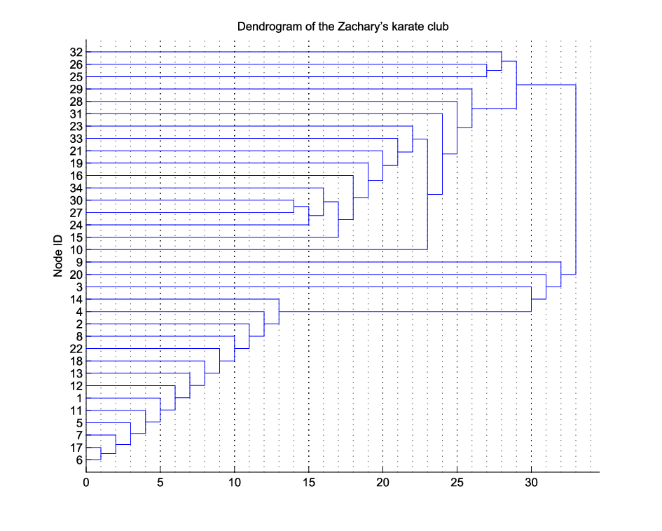
In Figure 6, we show the dendrogram generated by using our hierarchical agglomerative clustering algorithm with the greedy selection of the most cohesive pair in each iteration. The distance measure is the geodesic distance of the graph in Figure 3. The algorithm stops when there are three incohesive clusters left, one led by the administrator (node 34), one led by the instructor (node 1), and person number 9 himself. According to [41], there was an interesting story for person number 9. He was a weak supporter for the administrator. However, he was only three weeks away from a test for black belt (master status) when the split of the club occurred. He would have had to give up his rank if he had joined the administrator’s club. He ended up with the instructor’s club. We also run an additional step for our algorithm (to merge the pair with the largest cohesive measure) even though the remaining three clusters are incohesive. The additional step reveals that person number 9 is clustered into the instructor’s club.

IV A partitional algorithm

IV-A Triangular distance

In this section, we consider another objective function.

Definition 11

(normalized modularity) Let $S_{k}$ , $k=1,2,\ldots,K$ , be a partition of $\Omega=\{x_{1},x_{2},\ldots,x_{n}\}$ , i.e., $S_{k}\cap S_{k^{\prime}}$ is an empty set for $k\neq k^{\prime}$ and $\cup_{k=1}^{K}S_{k}=\Omega$ . The normalized modularity index $R$ with respect to the partition $S_{k}$ , $k=1,2,\ldots,K$ , is defined as follows:

R=\sum_{k=1}^{K}{1\over{|S_{k}|}}\gamma(S_{k},S_{k}).

(13)

Unlike the hierarchical agglomerative clustering algorithm in the previous section, in this section we assume that $K$ is fixed and known in advance. As such, we may use an approach similar to the classical $K$ -means algorithm by iteratively assigning each point to the nearest set (until it converges). Such an approach requires a measure that can measure how close a point $x$ to a set $S$ is. In the $K$ -means algorithm, such a measure is defined as the square of the distance between $x$ and the centroid of $S$ . However, there is no centroid for a set in a non-Euclidean space and we need to come up with another measure.

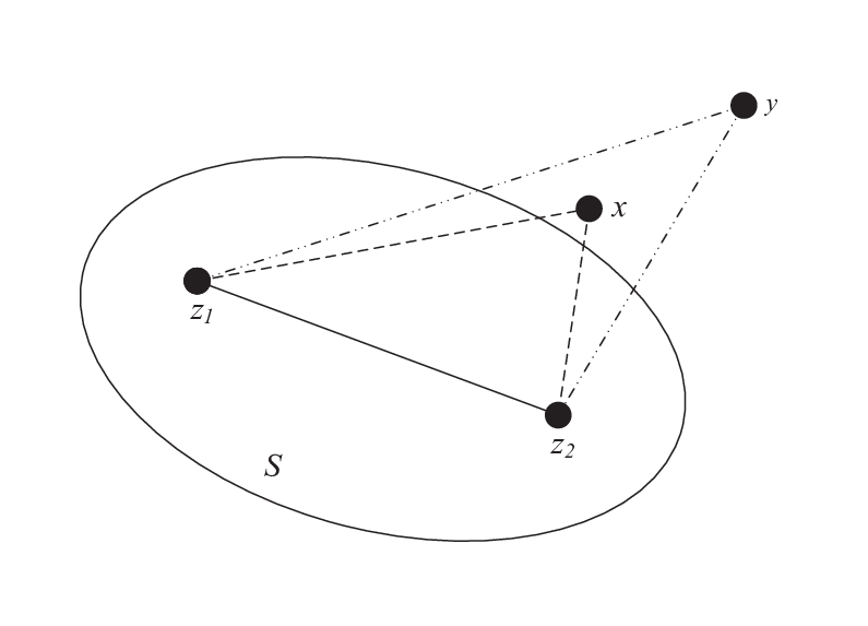
Our idea for measuring the distance from a point $x$ to a set $S$ is to randomly choose two points $z_{1}$ and $z_{2}$ from $S$ and consider the three sides of the triangle $x$ , $z_{1}$ and $z_{2}$ . Note that the triangular inequality guarantees that $d(x,z_{1})+d(x,z_{2})-d(z_{1},z_{2})\geq 0$ . Moreover, if $x$ is close to $z_{1}$ and $z_{2}$ , then $d(x,z_{1})+d(x,z_{2})-d(z_{1},z_{2})$ should also be small. We illustrate such an intuition in Figure 5, where there are two points $x$ and $y$ and a set $S$ in ${\cal R}^{2}$ . Such an intuition leads to the following definition of triangular distance from a point $x$ to a set $S$ .

Definition 12

(Triangular distance) The triangular distance from a point $x$ to a set $S$ , denoted by $\Delta(x,S)$ , is defined as follows:

\Delta(x,S)={1\over{|S|^{2}}}\sum_{z_{1}\in S}\sum_{z_{2}\in S}\Big(d(x,z_{1})+d(x,z_{2})-d(z_{1},z_{2})\Big).

(14)

In the following lemma, we show several properties of the triangular distance and its proof is given in Appendix D.

Lemma 13

(i)

\Delta(x,S)=2{\bar{d}}(\{x\},S)-{\bar{d}}(S,S)\geq 0.

(15)

(ii)

\Delta(x,S)=\gamma(x,x)-{2\over|S|}\gamma(\{x\},S)+{1\over{|S|^{2}}}\gamma(S,S).

(16)

(iii)

Let $S_{k}$ , $k=1,2,\ldots,K$ , be a partition of $\Omega=\{x_{1},x_{2},\ldots,x_{n}\}$ . Then

\sum_{k=1}^{K}\sum_{x\in S_{k}}\Delta(x,S_{k})=\sum_{x\in\Omega}\gamma(x,x)-R.

(17)

(iv)

Let $S_{k}$ , $k=1,2,\ldots,K$ , be a partition of $\Omega=\{x_{1},x_{2},\ldots,x_{n}\}$ and $c(x)$ be the index of the set to which $x$ belongs, i.e., $x\in S_{c(x)}$ . Then

	$\displaystyle\sum_{k=1}^{K}\sum_{x\in S_{k}}\Delta(x,S_{k})$	$\displaystyle=$	$\displaystyle\sum_{k=1}^{K}\sum_{x\in S_{k}}{\bar{d}}(\{x\},S_{k})$		(18)
		$\displaystyle=$	$\displaystyle\sum_{x\in\Omega}{\bar{d}}(\{x\},S_{c(x)}).$		(18)

The first property of this lemma is to represent triangular distance by the average distance. The second property is to represent the triangular distance by the cohesion measure. Such a property plays an important role for the duality result in Section V. The third property shows that the optimization problem for maximizing the normalized modularity $R$ is equivalent to the optimization problem that minimizes the sum of the triangular distance of each point to its set. The fourth property further shows that such an optimization problem is also equivalent to the optimization problem that minimizes the sum of the average distance of each point to its set. Note that ${\bar{d}}(\{x\},S_{k})={1\over{|S_{k}|}}\sum_{y\in S_{k}}d(x,y)$ . The objective for maximizing the normalized modularity $R$ is also equivalent to minimize

\sum_{k=1}^{K}{1\over{|S_{k}|}}\sum_{x\in S_{k}}\sum_{y\in S_{k}}d(x,y).

This is different from the $K$ -median objective, the $K$ -means objective and the min-sum objective addressed in [21].

IV-B The $K$ -sets algorithm

In the following, we propose a partitional clustering algorithm, called the $K$ -sets algorithm in Algorithm 2, based on the triangular distance. The algorithm is very simple. It starts from an arbitrary partition of the data points that contains $K$ disjoint sets. Then for each data point, we assign the data point to the closest set in terms of the triangular distance. We repeat the process until there is no further change. Unlike the Lloyd iteration that needs two-step minimization, the $K$ -sets algorithm only takes one-step minimization. This might give the $K$ -sets algorithm the computational advantage over the $K$ -medoids algorithms [6, 1, 7, 8].

ALGORITHM 2 The K-sets Algorithm

Input: A data set

\Omega=\{x_{1},x_{2},\ldots,x_{n}\}

, a distance measure

d(\cdot,\cdot)

, and the number of sets

K

Output: A partition of sets

\{S_{1},S_{2},\ldots,S_{K}\}

(0) Initially, choose arbitrarily

K

disjoint nonempty sets

S_{1},\ldots,S_{K}

as a partition of

\Omega

(1) for $i=1,2,\ldots,n$ do

Compute the triangular distance

\Delta(x_{i},S_{k})

for each set

S_{k}

by using (15).

Find the set to which the point

x_{i}

is closest in terms of the triangular distance.

Assign point

x_{i}

to that set.

end for

(2) Repeat from (1) until there is no further change.

In the following theorem, we show the convergence of the $K$ -sets algorithm. Moreover, for $K=2$ , the $K$ -sets algorithm yields two clusters. Its proof is given in Appendix E.

Theorem 14

(i): In the $K$ -sets algorithm based on the triangular distance, the normalized modularity is increasing when there is a change, i.e., a point is moved from one set to another. Thus, the algorithm converges to a local optimum of the normalized modularity.
(ii): Let $S_{1},S_{2},\ldots,S_{K}$ be the $K$ sets when the algorithm converges. Then for all $i\neq j$ , the two sets $S_{i}$ and $S_{j}$ are two clusters if these two sets are viewed in isolation (by removing the data points not in $S_{i}\cup S_{j}$ from $\Omega$ ).

An immediate consequence of Theorem 14 (ii) is that for $K=2$ , the two sets $S_{1}$ and $S_{2}$ are clusters when the algorithm converges. However, we are not able to show that for $K\geq 3$ the $K$ sets, $S_{1},S_{2},\ldots,S_{K}$ , are clusters in $\Omega$ . On the other hand, we are not able to find a counterexample either. All the numerical examples that we have tested for $K\geq 3$ yield $K$ clusters.

IV-C Experiments

In this section, we report several experimental results for the $K$ -sets algorithm: including the dataset with two rings in Section IV-C1, the stochastic block model in Section IV-C2, and the mixed National Institute of Standards and Technology dataset in Section IV-C3.

IV-C1 Two rings

In this section, we first provide an illustrating example for the $K$ -sets algorithm.

In Figure 6, we generate two rings by randomly placing 500 points in ${\cal R}^{2}$ . The outer (resp. inner) ring consists of 300 (resp. 200) points. The radius of a point in the outer (resp. inner) ring is uniformly distributed between 20 and 22 (resp. 10 and 12). The angle of each point is uniformly distributed between 0 and $2\pi$ . In Figure 6(a), we show a typical clustering result by using the classical $K$ -means algorithm with $K=2$ . As the centroids of these two rings are very close to each other, it is well-known that the $K$ -means algorithm does not perform well for the two rings. Instead of using the Euclidean distance as the distance measure for our $K$ -sets algorithm, we first convert the two rings into a graph by adding an edge between two points with the Euclidean distance less than 5. Then the distance measure between two points is defined as the geodesic distance of these two points in the graph. By doing so, we can then easily separate these rings by using the $K$ -sets algorithm with $K=2$ as shown in Figure 6(b).

The purpose of this example is to show the limitation of the applicability of the $K$ -means algorithm. The data points for the $K$ -means algorithm need to be in some Euclidean space. On the other hand, the data points for the $K$ -sets algorithms only need to be in some metric space. As such, the distance matrix constructed from a graph cannot be directly applied by the $K$ -means algorithm while it is still applicable for the $K$ -sets algorithm.

IV-C2 Stochastic block model

The stochastic block model (SBM), as a generalization of the Erdös-Rényi random graph [43], is a commonly used method for generating random graphs that can be used for benchmarking community detection algorithms [44, 45]. In a stochastic block model with $q$ blocks (communities), the total number of nodes in the random graph are evenly distributed to these $q$ blocks. The probability that there is an edge between two nodes within the same block is $p_{in}$ and the probability that there is an edge between two nodes in two different blocks is $p_{out}$ . These edges are generated independently. Let $c_{in}=n\cdot p_{in}$ , $c_{out}=n\cdot p_{out}$ . Then it is known [44] that these $q$ communities can be detected (in theory for a large network) if

|c_{in}-c_{out}|>q\sqrt{\text{mean degree}}.

(19)

In this paper, we use MODE-NET [45] to run SBM. Specifically, we consider a stochastic block model with two blocks. The number of nodes in the stochastic block model is 1,000 with 500 nodes in each of these two blocks. The average degree of a node is set to be 3. The values of $c_{in}-c_{out}$ of these graphs are in the range from 2.5 to 5.9 with a common step of 0.1. We generate 20 graphs for each $c_{in}-c_{out}$ . Isolated vertices are removed. Thus, the exact numbers of vertices used in this experiment are slightly less than than 1,000.

We compare our $K$ -sets algorithm with some other community detection algorithms, such as OSLOM2 [46], infomap [47, 48], and fast unfolding [38]. The metric used for the $K$ -sets algorithm for each sample of the random graph is the resistance distance, and this is pre-computed by NumPy [49]. The resistance distance matrix (denoted by $R=(R_{i,j})$ ) can be derived from the pseudo inverse of the adjacency matrix (denoted by $\Gamma=(\Gamma_{i,j})$ ) as follows: [50]:

R_{i,j}=\begin{cases}0,&\quad\text{if }i=j,\\ \Gamma_{i,i}+\Gamma_{j,j}-\Gamma_{i,j}-\Gamma_{j,i},&\quad\text{otherwise}.\\ \end{cases}

The $K$ -sets algorithm and OSLOM2 are implemented in C++, and the others are all taken from igraph [51] and are implemented in C with python wrappers. In Table II, we show the average running times for these four algorithms over 700 trials. The pre-computation time for the $K$ -sets algorithm is the time to compute the distance matrix. Except infomap, the other three algorithms are very fast. In Figure 7, we compute the normalized mutual information measure (NMI) by using a built-in function in igraph [51] for the results obtained from these four algorithms. Each point is averaged over 20 random graphs from the stochastic block model. The error bars are the 95% confidence intervals. In this stochastic block model, the theoretical phase transition threshold from (19) is $c_{in}-c_{out}=3.46$ . It seems that the $K$ -sets algorithm is able to detect these two blocks when $c_{in}-c_{out}\geq 4.5$ . Its performance in that range is better than infomap [47, 48], fast unfolding [38] and OSLOM2 [46]. We note that the comparison is not exactly fair as the other three algorithms do not have the information of the number of blocks (communities).

TABLE II: Average running time (in seconds).

pre-computation	0	0	0	2.3096
	infomap	fast unfolding	OSLOM2	$K$ -sets
running	0.7634	0.0074	0.0059	0.0060
total	0.7634	0.0074	0.0059	2.3156

IV-C3 Mixed National Institute of Standards and Technology dataset

In this section, we consider a real-world dataset, the mixed National Institute of Standards and Technology dataset (the MNIST dataset) [52]. The MNIST dataset contains 60,000 samples of hand-written digits. These samples are 28 $\times$ 28 pixels grayscale images (i.e., each of the image is a 784 dimensional data point). For our experiments, we select the first 1,000 samples from each set of the digit 0 to 9 to create a total number of 10,000 samples.

To fairly evaluate the performance of the $K$ -sets algorithm, we compare the $K$ -sets algorithm with two clustering algorithms in which the number of clusters is also known a priori, i.e., the $K$ -means++ algorithm [53] and the $K$ -medoids algorithm [54]. For the MNIST dataset, the number of clusters is 10 (for the ten digits, $0,1,2,\ldots,9$ ). The $K$ -means++ algorithm is an improvement of the standard $K$ -means algorithm with a specific method to choose the initial centroids of the $K$ clusters. Like the $K$ -sets algorithm, the $K$ -medoids algorithm is also a clustering algorithm that uses a distance measure. The key difference between the $K$ -sets algorithm and the $K$ -medoids algorithm is that we use the triangular distance to a set for the assignment of each data point and the $K$ -medoids algorithm uses the distance to a medoid for such an assignment. The Euclidean distance between two data points (samples from the MNIST dataset) for the $K$ -medoids algorithm and the $K$ -sets algorithm are pre-computed by NumPy [49]. The $K$ -sets algorithm is implemented in C++, and the others are implemented in C with python wrappers. All the programs are executed on an Acer Altos-T350-F2 machine with two Intel(R) Xeon(R) CPU E5-2690 v2 processors. In order to have a fair comparison of their running times, the parallelization of each program is disabled, i.e., only one core is used in these experiments. We assume that the input data is already stored in the main memory and the time consumed for I/O is not recorded.

In Table III, we show the average running times for these three algorithms over 100 trials. Both the $K$ -medoids algorithm and the $K$ -sets algorithm need to compute the distance matrix and this is shown in the row marked with the pre-computation time. The total running times for these three algorithms are roughly the same for this experiment. In Figure 8, we compute the normalized mutual information measure (NMI) by using a built-in function in igraph [51] for the results obtained from these three algorithms. Each point is averaged over 100 trials. The error bars are the 95% confidence intervals. In view of Figure 8, the $K$ -sets algorithm outperforms the $K$ -means++ algorithm and the $K$ -medoids algorithm for the MNIST dataset. One possible explanation for this is that both the the $K$ -means++ algorithm and the $K$ -medoids algorithm only select a single representative data point for a cluster and that representative data point may not be able to represent the whole cluster well enough. On the other hand, the $K$ -sets algorithm uses the triangular distance that takes the distance to every point in a cluster into account.

TABLE III: Average running time (in seconds).

	$K$ -means++	$K$ -medoids	$K$ -sets
pre-computation	0	36.981	36.981
running	49.940	1.228	1.801
total	49.940	38.209	38.782

V Duality between a cohesion measure and a distance measure

V-A The duality theorem

In this section, we show the duality result between a cohesion measure and a distance measure. In the following, we first provide a general definition for a cohesion measure.

Definition 15

A measure between two points $x$ and $y$ , denoted by $\beta(x,y)$ , is called a cohesion measure for a set of data points $\Omega$ if it satisfies the following three properties:

(C1)

(Symmetry) $\beta(x,y)=\beta(y,x)$ for all $x,y\in\Omega$ .

(C2)

(Zero-sum) For all $x\in\Omega$ , $\sum_{y\in\Omega}\beta(x,y)=0$ .

(C3)

(Triangular inequality) For all $x,y,z$ in $\Omega$ ,

\beta(x,x)+\beta(y,z)-\beta(x,z)-\beta(x,y)\geq 0.

(20)

In the following lemma, we show that the specific cohesion measure defined in Section II indeed satisfies (C1)–(C3) in Definition 15. Its proof is given in Appendix F.

Lemma 16

Suppose that $d(\cdot,\cdot)$ is a distance measure for $\Omega$ , i.e., $d(\cdot,\cdot)$ satisfies (D1)–(D4). Let

	$\displaystyle\beta(x,y)$	$\displaystyle=$	$\displaystyle{1\over n}\sum_{z_{2}\in\Omega}d(z_{2},y)+{1\over n}\sum_{z_{1}\in\Omega}d(x,z_{1})$		(21)
			$\displaystyle\quad-{1\over n^{2}}\sum_{z_{2}\in\Omega}\sum_{z_{1}\in\Omega}d(z_{2},z_{1})-d(x,y).$		(21)

Then $\beta(x,y)$ is a cohesion measure for $\Omega$ .

We know from (5) that the cohesion measure $\gamma(\cdot,\cdot)$ defined in Section II has the following representation:

	$\displaystyle\gamma(x,y)={1\over n}\sum_{z_{2}\in\Omega}d(z_{2},y)+{1\over n}\sum_{z_{1}\in\Omega}d(x,z_{1})$
	$\displaystyle\quad-{1\over n^{2}}\sum_{z_{2}\in\Omega}\sum_{z_{1}\in\Omega}d(z_{2},z_{1})-d(x,y).$

As a result of Lemma 16, it also satisfies (C1)–(C3) in Definition 15. As such, we call the cohesion measure $\gamma(\cdot,\cdot)$ defined in Section II the dual cohesion measure of the distance measure $d(\cdot,\cdot)$ .

On the other hand, if $\beta(x,y)$ is a cohesion measure for $\Omega$ , then there is an induced distance measure and it can be viewed as the dual distance measure of the cohesion measure $\beta(x,y)$ . This is shown in the following lemma and its proof is given in Appendix G.

Lemma 17

Suppose that $\beta(\cdot,\cdot)$ is a cohesion measure for $\Omega$ . Let

d(x,y)=(\beta(x,x)+\beta(y,y))/2-\beta(x,y).

(22)

Then $d(\cdot,\cdot)$ is a distance measure that satisfies (D1)–(D4).

In the following theorem, we show the duality result. Its proof is given in Appendix H.

Theorem 18

Consider a set of data points $\Omega$ . For a distance measure $d(\cdot,\cdot)$ that satisfies (D1)–(D4), let

	$\displaystyle d^{*}(x,y)={1\over n}\sum_{z_{2}\in\Omega}d(z_{2},y)+{1\over n}\sum_{z_{1}\in\Omega}d(x,z_{1})$
	$\displaystyle\quad-{1\over n^{2}}\sum_{z_{2}\in\Omega}\sum_{z_{1}\in\Omega}d(z_{2},z_{1})-d(x,y)$		(23)

be the dual cohesion measure of $d(\cdot,\cdot)$ . On the other hand, For a cohesion measure $\beta(\cdot,\cdot)$ that satisfies (C1)–(C3), let

\beta^{*}(x,y)=(\beta(x,x)+\beta(y,y))/2-\beta(x,y)

(24)

be the dual distance measure of $\beta(\cdot,\cdot)$ . Then $d^{**}(x,y)=d(x,y)$ and $\beta^{**}(x,y)=\beta(x,y)$ for all $x,y\in\Omega$ .

V-B The dual $K$ -sets algorithm

For the $K$ -sets algorithm, we need to have a distance measure. In view of the duality theorem between a cohesion measure and a distance measure, we propose the dual $K$ -sets algorithm in Algorithm 3 that uses a cohesion measure. As before, for a cohesion measure $\gamma(\cdot,\cdot)$ between two points, we define the cohesion measure between two sets $S_{1}$ and $S_{2}$ as

\gamma(S_{1},S_{2})=\sum_{x\in S_{1}}\sum_{y\in S_{2}}\gamma(x,y).

(25)

Also, note from (16) that the triangular distance from a point $x$ to a set $S$ can be computed by using the cohesion measure as follows:

\Delta(x,S)=\gamma(x,x)-{2\over{|S|}}\gamma(\{x\},S)+{1\over{|S|^{2}}}\gamma(S,S).

(26)

ALGORITHM 3 The dual K-sets Algorithm

Input: A data set

\Omega=\{x_{1},x_{2},\ldots,x_{n}\}

, a cohesion measure

\gamma(\cdot,\cdot)

, and the number of sets

K

Output: A partition of sets

\{S_{1},S_{2},\ldots,S_{K}\}

(0) Initially, choose arbitrarily

K

disjoint nonempty sets

S_{1},\ldots,S_{K}

as a partition of

\Omega

(1) for $i=1,2,\ldots,n$ do

Compute the triangular distance

\Delta(x_{i},S_{k})

for each set

S_{k}

by using (26).

Find the set to which the point

x_{i}

is closest in terms of the triangular distance.

Assign point

x_{i}

to that set.

end for

(2) Repeat from (1) until there is no further change.

As a direct result of the duality theorem in Theorem 18 and the convergence result of the $K$ -sets algorithm in Theorem 14, we have the following convergence result for the dual $K$ -sets algorithm.

Corollary 19

As in (13), we define the normalized modularity as $\sum_{k=1}^{K}{1\over{|S_{k}|}}\gamma(S_{k},S_{k})$ . For the dual $K$ -sets algorithm, the normalized modularity is increasing when there is a change, i.e., a point is moved from one set to another. Thus, the algorithm converges to a local optimum of the normalized modularity. Moreover, for $K=2$ , the dual $K$ -sets algorithm yields two clusters when the algorithm converges.

V-C Connections to the kernel $K$ -means algorithm

In this section, we show the connection between the dual $K$ -sets algorithm and the kernel $K$ -means algorithm in the literature (see e.g., [55]). Let us consider the $n\times n$ matrix $\Gamma=(\gamma_{i,j})$ with $\gamma_{i,j}=\gamma(x_{i},x_{j})$ being the cohesion measure between $x_{i}$ and $x_{j}$ . Call the matrix $\Gamma$ the cohesion matrix (corresponding to the cohesion measure $\gamma(\cdot,\cdot)$ ). Since $\gamma(x_{i},x_{j})=\gamma(x_{j},x_{i})$ , the matrix $\Gamma$ is symmetric and thus have real eigenvalues $\lambda_{k},k=1,2,\ldots,n$ . Let $\bf I$ be the $n\times n$ identity matrix and $\sigma\geq-\min_{1\leq k\leq n}{\lambda_{k}}$ . Then the matrix $\tilde{\Gamma}=\sigma{\bf I}+\Gamma$ is positive semi-definite as its $n$ eigenvalues $\tilde{\lambda}_{k}=\sigma+\lambda_{k}$ , $k=1,2,\ldots,N$ are all nonnegative. Let $v_{k}=(v_{k,1},v_{k,2},\ldots,v_{k,n})^{T}$ , $k=1,2,\ldots,n$ be the eigenvector of $\Gamma$ corresponding to the eigenvalue $\lambda_{k}$ . Then $v_{k}$ is also the eigenvector of $\tilde{\Gamma}$ corresponding to the eigenvalue $\tilde{\lambda}_{k}$ . Thus, we can decompose the matrix $\tilde{\Gamma}$ as follows:

\tilde{\Gamma}=\sum_{k=1}^{n}\tilde{\lambda}_{k}v_{k}v_{k}^{T},

(27)

where $v_{k}^{T}$ is the transpose of $v_{k}$ . Now we choose the mapping $\phi:\Omega\mapsto{\cal R}^{n}$ as follows:

\phi(x_{i})=\Big(\sqrt{\tilde{\lambda}_{1}}v_{1,i},\sqrt{\tilde{\lambda}_{2}}v_{2,i},\ldots,\sqrt{\tilde{\lambda}_{n}}v_{n,i}\Big)^{T},

(28)

for $i=1,2\ldots,n$ . Note that

	$\displaystyle\phi(x_{i})^{T}\cdot\phi(x_{j})$	$\displaystyle=$	$\displaystyle\sum_{k=1}^{n}\tilde{\lambda}_{k}v_{k,i}v_{k,j}$		(29)
		$\displaystyle=$	$\displaystyle(\tilde{\Gamma})_{i,j}=\sigma\delta_{i,j}+\gamma(x_{i},x_{j}),$		(29)

where $\delta_{i,j}=1$ if $i=j$ and 0 otherwise.

The “centroid” of a set $S$ can be represented by the corresponding centroid in ${\cal R}^{n}$ , i.e.,

{1\over|S|}\sum_{y\in S}\phi(y),

(30)

and the square of the “distance” between a point $x$ and the “centroid” of a set $S$ is

	$\displaystyle\Big(\phi(x)-{1\over{\|S\|}}\sum_{y\in S}\phi(y)\Big)^{T}\cdot\Big(\phi(x)-{1\over{\|S\|}}\sum_{y\in S}\phi(y)\Big)$
	$\displaystyle=\phi(x)^{T}\cdot\phi(x)-{2\over{\|S\|}}\sum_{y\in S}\phi(x)^{T}\cdot\phi(y)$
	$\displaystyle\quad\quad+{1\over{\|S\|^{2}}}\sum_{y_{1}\in S}\sum_{y_{2}\in S}\phi(y_{1})^{T}\cdot\phi(y_{2})$
	$\displaystyle=\gamma(x,x)+\sigma-{2\over{\|S\|}}\sum_{y\in S}\gamma(x,y)-{{2\sigma}\over{\|S\|}}1_{\{x\in S\}}$
	$\displaystyle\quad\quad+{1\over{\|S\|^{2}}}\sum_{y_{1}\in S}\sum_{y_{2}\in S}\gamma(y_{1},y_{2})+{{\|S\|\sigma}\over{\|S\|^{2}}}$
	$\displaystyle=(1-{{2}\over{\|S\|}}1_{\{x\in S\}}+{1\over{\|S\|}})\sigma+\gamma(x,x)-{2\over{\|S\|}}\gamma(\{x\},S)$
	$\displaystyle\quad\quad+{1\over{\|S\|^{2}}}\gamma(S,S),$		(31)

where $1_{\{x\in S\}}$ is the indicator function that has value 1 if $x$ is in $S$ and 0 otherwise. In view of (16), we then have

	$\displaystyle\Big(\phi(x)-{1\over{\|S\|}}\sum_{y\in S}\phi(y)\Big)^{T}\cdot\Big(\phi(x)-{1\over{\|S\|}}\sum_{y\in S}\phi(y)\Big)$
	$\displaystyle=(1-{{2}\over{\|S\|}}1_{\{x\in S\}}+{1\over{\|S\|}})\sigma+\Delta(x,S),$		(32)

where $\Delta(x,S)$ is the triangular distance from a point $x$ to a set $S$ . Thus, the square of the “distance” between a point $x$ and the “centroid” of a set $S$ is $(1-{1\over{|S|}})\sigma+\Delta(x,S)$ for a point $x\in S$ and $(1+{1\over{|S|}})\sigma+\Delta(x,S)$ for a point $x\not\in S$ . In particular, when $\sigma=0$ , the dual $K$ -sets algorithm is the same as the sequential kernel $K$ -means algorithm for the kernel $\tilde{\Gamma}$ . Unfortunately, the matrix $\tilde{\Gamma}$ may not be positive semi-definite if $\sigma$ is chosen to be 0. As indicated in [55], a large $\sigma$ decreases (resp. increases) the distance from a point $x$ to a set $S$ that contains (resp. does not contain) that point. As such, a point is more unlikely to move from one set to another set and the kernel $K$ -means algorithm is thus more likely to be trapped in a local optimum.

To summarize, the dual $K$ -sets algorithm operates in the same way as a sequential version of the classical kernel $K$ -means algorithm by viewing the matrix $\Gamma$ as a kernel. However, there are two key differences between the dual $K$ -sets algorithm and the classical kernel $K$ -means algorithm: (i) the dual $K$ -sets algorithm guarantees the convergence even though the matrix $\Gamma$ from a cohesion measure is not positive semi-definite, and (ii) the dual $K$ -sets algorithm can only be operated sequentially and the kernel $K$ -means algorithm can be operated in batches. To further illustrate the difference between these two algorithms, we show in the following two examples that a cohesion matrix may not be positive semi-definite and a positive semi-definite matrix may not be a cohesion matrix.

Example 20

In this example, we show there is a cohesion matrix $\Gamma$ that is not a positive semi-definite matrix.

{\Gamma}=\left(\begin{array}[]{rrrrr}0.44&0.04&0.04&0.04&-0.56\\ 0.04&0.64&-0.36&-0.36&0.04\\ 0.04&-0.36&0.64&-0.36&0.04\\ 0.04&-0.36&-0.36&0.64&0.04\\ -0.56&0.04&0.04&0.04&0.44\end{array}\right).

(33)

The eigenvalues of this matrix are $-0.2$ , $0$ , $1$ , $1$ , and $1$ .

Example 21

In this example, we show there is a positive semi-definite matrix $M=(m_{i,j})$ that is not an cohesion matrix.

M=\left(\begin{array}[]{rrrr}0.375&-0.025&-0.325&-0.025\\ -0.025&0.875&-0.025&-0.825\\ -0.325&-0.025&0.375&-0.025\\ -0.025&-0.825&-0.025&0.875\end{array}\right).

(34)

The eigenvalues of this matrix are $0$ , $0.1$ , $0.7$ , and $1.7$ . Even though the matrix $M$ is symmetric and has all its row sums and column sums being 0, it is still not a cohesion matrix as $m_{1,1}-m_{1,2}-m_{1,4}+m_{2,4}=-0.4<0$ .

V-D Constructing a cohesion measure from a similarity measure

A similarity measure is in general defined as a bivariate function of two distinct data points and it is often characterized by a square matrix without specifying the diagonal elements. In the following, we show how one can construct a cohesion measure from a symmetric bivariate function by further specifying the diagonal elements. Its proof is given in Appendix I.

Proposition 22

Suppose a bivariate function $\beta_{0}:\Omega\times\Omega\mapsto{\cal R}$ is symmetric, i.e., $\beta_{0}(x,y)=\beta_{0}(y,x)$ . Let $\beta_{1}(x,y)=\beta_{0}(x,y)$ for all $x\neq y$ and specify $\beta_{1}(x,x)$ such that

\beta_{1}(x,x)\geq\max_{x\neq y\neq z}[\beta_{1}(x,z)+\beta_{1}(x,y)-\beta_{1}(y,z)].

(35)

Also, let

	$\displaystyle\beta(x,y)=\beta_{1}(x,y)-{1\over n}\sum_{z_{1}\in\Omega}\beta_{1}(z_{1},y)$
	$\displaystyle\quad-{1\over n}\sum_{z_{2}\in\Omega}\beta_{1}(x,z_{2})+{1\over{n^{2}}}\sum_{z_{1}\in\Omega}\sum_{z_{2}\in\Omega}\beta_{1}(z_{1},z_{2}).$		(36)

Then $\beta(x,y)$ is a cohesion measure for $\Omega$ .

We note that one simple choice for specifying $\beta_{1}(x,x)$ in (35) is to set

\beta_{1}(x,x)=2\beta_{\max}-\beta_{\min},

(37)

where

\beta_{\max}=\max_{x\neq y}\beta(x,y),

(38)

and

\beta_{\min}=\min_{x\neq y}\beta(x,y).

(39)

In particular, if the similarity measure $\beta(x,y)$ only has values 0 and 1 as in the adjacency matrix of a simple undirected graph, then one can simply choose $\beta_{1}(x,x)=2$ for all $x$ .

Example 23

(A cohesion measure for a graph) As an illustrating example, suppose $A=(a_{i,j})$ is the $n\times n$ adjacency matrix of a simple undirected graph with $a_{i,j}=1$ if there is an edge between node $i$ and node $j$ and 0 otherwise. Let $k_{i}=\sum_{j=1}^{n}a_{i,j}$ be the degree of node $i$ and $m={1\over 2}\sum_{i=1}^{n}k_{i}$ be the total number of edges in the graph. Then one can simply let $\beta_{1}(i,j)=2\delta_{i,j}+a_{i,j}$ , where $\delta_{i,j}=1$ if $i=j$ and 0 otherwise. By doing so, we then have the following cohesion measure

\beta(i,j)=2\delta_{i,j}+a_{i,j}-{{2+k_{i}}\over n}-{{2+k_{j}}\over n}+{{2m+2n}\over{n^{2}}}.

(40)

We note that such a cohesion measure is known as the deviation to indetermination null model in [56].

VI Conclusions

In this paper, we developed a mathematical theory for clustering in metric spaces based on distance measures and cohesion measures. A cluster is defined as a set of data points that are cohesive to themselves. The hierarchical agglomerative algorithm in Algorithm 1 was shown to converge with a partition of clusters. Our hierarchical agglomerative algorithm differs from a standard hierarchical agglomerative algorithm in two aspects: (i) there is a stopping criterion for our algorithm, and (ii) there is no need to use the greedy selection. We also proposed the $K$ -sets algorithm in Algorithm 2 based on the concept of triangular distance. Such an algorithm appears to be new. Unlike the Lloyd iteration, it only takes one-step minimization in each iteration and that might give the $K$ -sets algorithm the computational advantage over the $K$ -medoids algorithms. The $K$ -sets algorithm was shown to converge with a partition of two clusters when $K=2$ . Another interesting finding of the paper is the duality result between a distance measure and a cohesion measure. As such, one can perform clustering either by a distance measure or a cohesion measure. In particular, the dual $K$ -sets algorithm in Algorithm 3 converges in the same way as a sequential version of the kernel $K$ -means algorithm without the need for the cohesion matrix to positive semi-definite.

There are several possible extensions for our work:

(i) Asymmetric distance measure: One possible extension is to remove the symmetric property in (D3) for a distance measure. Our preliminary result shows that one only needs $d(x,x)=0$ in (D2) and the triangular inequality in (D4) for the $K$ -sets algorithm to converge. The key insight for this is that one can replace the original distance measure $d(x,y)$ by a new distance measure $\tilde{d}(x,y)=d(x,y)+d(y,x)$ . By doing so, the new distance measure is symmetric.

(ii) Distance measure without the triangular inequality: Another possible extension is to remove the triangular inequality in (D4). However, the $K$ -sets algorithm does not work properly in this setting as the triangular distance is no longer nonnegative. In order for the $K$ -sets algorithm to converge, our preliminary result shows that one can adjust the value of the triangular distance based on a weaker notion of cohesion measure. Results along this line will be reported separately.

(iii) Performance guarantee: Like the $K$ -means algorithm, the output of the $K$ -sets algorithm also depends on the initial partition. It would be of interest to see if it is possible to derive performance guarantee for the $K$ -sets algorithm (or the optimization problem for the normalized modularity). In particular, the approach by approximation stability in [21] might be applicable as their threshold graph lemma seems to hold when one replaces the distance from a point $x$ to its center $c$ , i.e., $d(x,c)$ , by the average distance of a point $x$ to its set, i.e., ${\bar{d}}(x,S)$ .

(iv) Local clustering: The problem of local clustering is to find a cluster that contains a specific point $x$ . Since we already define what a cluster is, we may use the hierarchical agglomerative algorithm in Algorithm 1 to find a cluster that contains $x$ . One potential problem of such an approach is the output cluster might be very big. Analogous to the concept of community strength in [34], it would be of interest to define a concept of cluster strength and stop the agglomerative process when the desired cluster strength can no longer be met.

(v) Reduction of computational complexity: Note that the computation complexity for each iteration within the FOR loop of the $K$ -sets algorithm is $O(Kn^{2})$ as it takes $O(Kn)$ steps to compute the triangular distance for each point and there are $n$ points that need to be assigned in each iteration. To further reduce the computational complexity for such an algorithm, one might exploit the idea of “sparsity” and this can be done by the transformation of distance measure.

Acknowledgement

This work was supported in part by the Excellent Research Projects of National Taiwan University, under Grant Number AE00-00-04, and in part by National Science Council (NSC), Taiwan, under Grant Numbers NSC102-2221-E-002-014-MY2 and 102-2221-E-007 -006 -MY3.

References

[1] Sergios Theodoridis and Konstantinos Koutroumbas. Pattern Recognition. Elsevier Academic press, USA, 2006.
[2] Anand Rajaraman, Jure Leskovec, and Jeffrey David Ullman. Mining of massive datasets. Cambridge University Press, 2012.
[3] Anil K Jain, M Narasimha Murty, and Patrick J Flynn. Data clustering: a review. ACM computing surveys (CSUR), 31(3):264–323, 1999.
[4] Anil K Jain. Data clustering: 50 years beyond k-means. Pattern Recognition Letters, 31(8):651–666, 2010.
[5] Stuart Lloyd. Least squares quantization in pcm. Information Theory, IEEE Transactions on, 28(2):129–137, 1982.
[6] Leonard Kaufman and Peter J Rousseeuw. Finding groups in data: an introduction to cluster analysis, volume 344. John Wiley & Sons, 2009.
[7] Mark Van der Laan, Katherine Pollard, and Jennifer Bryan. A new partitioning around medoids algorithm. Journal of Statistical Computation and Simulation, 73(8):575–584, 2003.
[8] Hae-Sang Park and Chi-Hyuck Jun. A simple and fast algorithm for k-medoids clustering. Expert Systems with Applications, 36(2):3336–3341, 2009.
[9] Sariel Har-Peled and Bardia Sadri. How fast is the k-means method? Algorithmica, 41(3):185–202, 2005.
[10] David Arthur and Sergei Vassilvitskii. k-means++: The advantages of careful seeding. In Proceedings of the eighteenth annual ACM-SIAM symposium on Discrete algorithms, pages 1027–1035. Society for Industrial and Applied Mathematics, 2007.
[11] Bahman Bahmani, Benjamin Moseley, Andrea Vattani, Ravi Kumar, and Sergei Vassilvitskii. Scalable k-means++. Proceedings of the VLDB Endowment, 5(7):622–633, 2012.
[12] Ragesh Jaiswal and Nitin Garg. Analysis of k-means++ for separable data. In Approximation, Randomization, and Combinatorial Optimization. Algorithms and Techniques, pages 591–602. Springer, 2012.
[13] Manu Agarwal, Ragesh Jaiswal, and Arindam Pal. k-means++ under approximation stability. In Theory and Applications of Models of Computation, pages 84–95. Springer, 2013.
[14] Jianbo Shi and Jitendra Malik. Normalized cuts and image segmentation. Pattern Analysis and Machine Intelligence, IEEE Transactions on, 22(8):888–905, 2000.
[15] Asa Ben-Hur, David Horn, Hava T Siegelmann, and Vladimir Vapnik. Support vector clustering. The Journal of Machine Learning Research, 2:125–137, 2002.
[16] Chris Ding and Xiaofeng He. K-means clustering via principal component analysis. In Proceedings of the twenty-first international conference on Machine learning, page 29. ACM, 2004.
[17] Francesco Camastra and Alessandro Verri. A novel kernel method for clustering. Pattern Analysis and Machine Intelligence, IEEE Transactions on, 27(5):801–805, 2005.
[18] Wen-Yen Chen, Yangqiu Song, Hongjie Bai, Chih-Jen Lin, and Edward Y Chang. Parallel spectral clustering in distributed systems. Pattern Analysis and Machine Intelligence, IEEE Transactions on, 33(3):568–586, 2011.
[19] Ulrike Von Luxburg. A tutorial on spectral clustering. Statistics and computing, 17(4):395–416, 2007.
[20] Maurizio Filippone, Francesco Camastra, Francesco Masulli, and Stefano Rovetta. A survey of kernel and spectral methods for clustering. Pattern recognition, 41(1):176–190, 2008.
[21] Maria-Florina Balcan, Avrim Blum, and Anupam Gupta. Clustering under approximation stability. Journal of the ACM (JACM), 60(2):8, 2013.
[22] Ulrike Von Luxburg and Shai Ben-David. Towards a statistical theory of clustering. In Pascal workshop on statistics and optimization of clustering. Citeseer, 2005.
[23] Nicholas Jardine and Robin Sibson. Mathematical taxonomy. London etc.: John Wiley, 1971.
[24] William E Wright. A formalization of cluster analysis. Pattern Recognition, 5(3):273–282, 1973.
[25] Jan Puzicha, Thomas Hofmann, and Joachim M Buhmann. A theory of proximity based clustering: Structure detection by optimization. Pattern Recognition, 33(4):617–634, 2000.
[26] Jon Kleinberg. An impossibility theorem for clustering. Advances in neural information processing systems, pages 463–470, 2003.
[27] Reza Bosagh Zadeh and Shai Ben-David. A uniqueness theorem for clustering. In Proceedings of the twenty-fifth conference on uncertainty in artificial intelligence, pages 639–646. AUAI Press, 2009.
[28] Gunnar Carlsson, Facundo Mémoli, Alejandro Ribeiro, and Santiago Segarra. Hierarchical quasi-clustering methods for asymmetric networks. arXiv preprint arXiv:1404.4655, 2014.
[29] Shai Ben-David and Margareta Ackerman. Measures of clustering quality: A working set of axioms for clustering. In Advances in neural information processing systems, pages 121–128, 2009.
[30] Martin Ester, Hans-Peter Kriegel, Jörg Sander, and Xiaowei Xu. A density-based algorithm for discovering clusters in large spatial databases with noise. In Kdd, volume 96, pages 226–231, 1996.
[31] Antonio Cuevas, Manuel Febrero, and Ricardo Fraiman. Cluster analysis: a further approach based on density estimation. Computational Statistics & Data Analysis, 36(4):441–459, 2001.
[32] Maria Halkidi and Michalis Vazirgiannis. A density-based cluster validity approach using multi-representatives. Pattern Recognition Letters, 29(6):773–786, 2008.
[33] David Liben-Nowell and Jon Kleinberg. The link prediction problem for social networks. In Proceedings of the twelfth international conference on Information and knowledge management, pages 556–559. ACM, 2003.
[34] Cheng-Shang Chang, Chih-Jung Chang, Wen-Ting Hsieh, Duan-Shin Lee, Li-Heng Liou, and Wanjiun Liao. Relative centrality and local community detection. Network Science, FirstView:1–35, 8 2015.
[35] Ulrik Brandes, Daniel Delling, Marco Gaertler, Robert Gorke, Martin Hoefer, Zoran Nikoloski, and Dorothea Wagner. On modularity clustering. Knowledge and Data Engineering, IEEE Transactions on, 20(2):172–188, 2008.
[36] Mark EJ Newman. Fast algorithm for detecting community structure in networks. Physical review E, 69(6):066133, 2004.
[37] Mark EJ Newman and Michelle Girvan. Finding and evaluating community structure in networks. Physical review E, 69(2):026113, 2004.
[38] Vincent D Blondel, Jean-Loup Guillaume, Renaud Lambiotte, and Etienne Lefebvre. Fast unfolding of communities in large networks. Journal of Statistical Mechanics: Theory and Experiment, 2008(10):P10008, 2008.
[39] Renaud Lambiotte. Multi-scale modularity in complex networks. In Modeling and Optimization in Mobile, Ad Hoc and Wireless Networks (WiOpt), 2010 Proceedings of the 8th International Symposium on, pages 546–553. IEEE, 2010.
[40] J-C Delvenne, Sophia N Yaliraki, and Mauricio Barahona. Stability of graph communities across time scales. Proceedings of the National Academy of Sciences, 107(29):12755–12760, 2010.
[41] Wayne W Zachary. An information flow model for conflict and fission in small groups. Journal of anthropological research, pages 452–473, 1977.
[42] Cheng-Shang Chang, Chin-Yi Hsu, Jay Cheng, and Duan-Shin Lee. A general probabilistic framework for detecting community structure in networks. In IEEE INFOCOM ’11, April 2011.
[43] P. Erdös and A. Rényi. On random graphs. Publ. Math. Debrecen, 6:290–297, 1959.
[44] Alaa Saade, Florent Krzakala, and Lenka Zdeborová. Spectral clustering of graphs with the bethe hessian. In Advances in Neural Information Processing Systems, pages 406–414, 2014.
[45] Lenka Zdeborova Aurelien Decelle, Florent Krzakala and Pan Zhang. Mode-net: Modules detection in networks, 2012.
[46] Andrea Lancichinetti, Filippo Radicchi, José J Ramasco, Santo Fortunato, et al. Finding statistically significant communities in networks. PloS one, 6(4):e18961, 2011.
[47] M. Rosvall and C. T. Bergstrom. Maps of information flow reveal community structure in complex networks. Technical report, Citeseer, 2007.
[48] Martin Rosvall, Daniel Axelsson, and Carl T Bergstrom. The map equation. The European Physical Journal Special Topics, 178(1):13–23, 2010.
[49] Stefan Van Der Walt, S Chris Colbert, and Gael Varoquaux. The numpy array: a structure for efficient numerical computation. Computing in Science & Engineering, 13(2):22–30, 2011.
[50] Ravindra B Bapat, Ivan Gutmana, and Wenjun Xiao. A simple method for computing resistance distance. Zeitschrift für Naturforschung A, 58(9-10):494–498, 2003.
[51] Gabor Csardi and Tamas Nepusz. The igraph software package for complex network research. InterJournal, Complex Systems:1695, 2006.
[52] Yann LeCun and Corinna Cortes. MNIST handwritten digit database. http://yann.lecun.com/exdb/mnist/, 2010.
[53] F. Pedregosa, G. Varoquaux, A. Gramfort, V. Michel, B. Thirion, O. Grisel, M. Blondel, P. Prettenhofer, R. Weiss, V. Dubourg, J. Vanderplas, A. Passos, D. Cournapeau, M. Brucher, M. Perrot, and E. Duchesnay. Scikit-learn: Machine learning in Python. Journal of Machine Learning Research, 12:2825–2830, 2011.
[54] Kyle A Beauchamp, Gregory R Bowman, Thomas J Lane, Lutz Maibaum, Imran S Haque, and Vijay S Pande. Msmbuilder2: Modeling conformational dynamics on the picosecond to millisecond scale. Journal of chemical theory and computation, 7(10):3412–3419, 2011.
[55] Inderjit Dhillon, Yuqiang Guan, and Brian Kulis. A unified view of kernel k-means, spectral clustering and graph cuts. Computer Science Department, University of Texas at Austin, 2004.
[56] Romain Campigotto, Patricia Conde Céspedes, and Jean-Loup Guillaume. A generalized and adaptive method for community detection. arXiv preprint arXiv:1406.2518, 2014.

Appendix A

In this section, we prove Proposition 4.

(i) Since the distance measure $d(\cdot,\cdot)$ is symmetric, we have from (5) that $\gamma(x,y)=\gamma(y,x)$ . Thus, the cohesion measure between two points is symmetric.

(ii) We note from (6) that

	$\displaystyle\gamma(x,x)$	$\displaystyle=$	$\displaystyle{1\over n^{2}}\sum_{z_{2}\in\Omega}\sum_{z_{1}\in\Omega}\Big(d(x,z_{1})+d(z_{2},x)$		(41)
			$\displaystyle\quad\quad-d(z_{1},z_{2})-d(x,x)\Big).$		(41)

Since $d(x,x)=0$ , we have from the triangular inequality that $\gamma(x,x)\geq 0$ .

(iii) Note from (41) and (6) that

	$\displaystyle\gamma(x,x)-\gamma(x,y)$
	$\displaystyle={1\over n}\sum_{z_{2}\in\Omega}\Big(d(z_{2},x)-d(x,x)+d(x,y)-d(z_{2},y)\Big).$

Since $d(x,x)=0$ , we have from the triangular inequality that

\gamma(x,x)\geq\gamma(x,y).

(iv) This can be easily verified by summing $y$ in (5).

Appendix B

In this section, we prove Theorem 7.

We first list several properties for the average distance that will be used in the proof of Theorem 7.

Fact 24

(i)

${\bar{d}}(S_{1},S_{2})\geq 0$ ;

(ii)

(Symmetry) ${\bar{d}}(S_{1},S_{2})={\bar{d}}(S_{2},S_{1})$ ;

(iii)

(Weighted average) Suppose that $S_{2}$ and $S_{3}$ are two disjoint subsets of $\Omega$ . Then

	$\displaystyle{\bar{d}}(S_{1},S_{2}\cup S_{3})$
	$\displaystyle={{\|S_{2}\|}\over{\|S_{2}\|+{\|S_{3}\|}}}{\bar{d}}(S_{1},S_{2})+{{\|S_{3}\|}\over{\|S_{2}\|+{\|S_{3}\|}}}{\bar{d}}(S_{1},S_{3}).$

Now we can use the average distance to represent the relative distance and the cohesion measure.

Fact 25

(i)

From (5), one can represent the cohesion measure between two points in terms of the average distance as follows:

\gamma(x,y)={\bar{d}}(\Omega,y)+{\bar{d}}(x,\Omega)-{\bar{d}}(\Omega,\Omega)-d(x,y).

(43)

(ii)

From (8) and (43), one can represent the cohesion measure between two sets in terms of the average distance as follows:

	$\displaystyle\gamma(S_{1},S_{2})$	$\displaystyle=$	$\displaystyle\|S_{1}\|\cdot\|S_{2}\|\cdot\Big({\bar{d}}(\Omega,S_{2})+{\bar{d}}(S_{1},\Omega)$		(44)
			$\displaystyle\quad-{\bar{d}}(\Omega,\Omega)-{\bar{d}}(S_{1},S_{2})\Big).$		(44)

(iii)

From (1), one can represent the relative distance from $x$ to $y$ in terms of the average distance as follows:

\mbox{RD}(x||y)=d(x,y)-{\bar{d}}(x,\Omega).

(45)

(iv)

From (45) and (3), one can represent the relative distance from set $S_{1}$ to another set $S_{2}$ in terms of the average distance as follows:

\mbox{RD}(S_{1}||S_{2})={\bar{d}}(S_{1},S_{2})-{\bar{d}}(S_{1},\Omega).

(46)

Using the representation of the cohesion measure by the average distance, we show some properties for the cohesion measure between two sets in the following proposition.

Proposition 26

(i)

(Symmetry) For any two sets $S_{1}$ and $S_{2}$ ,

\gamma(S_{1},S_{2})=\gamma(S_{2},S_{1}).

(47)

(ii)

(Zero-sum) Any set $S$ is both cohesive and incohesive to $\Omega$ , i.e., $\gamma(\Omega,S)=\gamma(S,\Omega)=0$ .

(iii)

(Union of two disjoint sets) Suppose that $S_{2}$ and $S_{3}$ are two disjoint subsets of $\Omega$ . Then for any set $S_{1}$

\gamma(S_{1},S_{2}\cup S_{3})=\gamma(S_{1},S_{2})+\gamma(S_{1},S_{3}).

(48)

(iv)

(Union of two disjoint sets) Suppose that $S_{2}$ and $S_{3}$ are two disjoint subsets of $\Omega$ . Then for any set $S_{1}$

\gamma(S_{2}\cup S_{3},S_{1})=\gamma(S_{2},S_{1})+\gamma(S_{3},S_{1}).

(49)

(v)

Suppose that $S$ is a nonempty set and it is not equal to $\Omega$ . Let $S^{c}=\Omega\backslash S$ be the set of points that are not in $S$ . Then

\gamma(S,S)=-\gamma(S^{c},S)=\gamma(S^{c},S^{c}).

(50)

Proof. (i) The symmetric property follows from the symmetric property of $\gamma(x,y)$ .

(ii) That $\gamma(\Omega,S)=0$ follows trivially from (44).

(iii) This is a direct consequence of the definition in (8).

(iv) That (49) holds follows from the symmetric property in (i) and the identity in (48).

(v) Note from (ii) of this proposition that $\gamma(\Omega,S)=\gamma(S\cup S^{c},S)=0$ . Using (49) yields

\gamma(S,S)+\gamma(S^{c},S)=0.

Thus, we have

\gamma(S,S)=-\gamma(S^{c},S).

(51)

From (51), we also have

\gamma(S^{c},S^{c})=-\gamma(S,S^{c}).

(52)

From the symmetric property in (i) of this proposition, we have $\gamma(S^{c},S)=\gamma(S,S^{c})$ . As a result of (51) and (52), we then have

\gamma(S,S)=\gamma(S^{c},S^{c}).

Using the representations of the relative distance and the cohesion measure by the average distance, we show some properties for the relative distance in the following proposition.

Proposition 27

(i)

(Zero-sum) The relative distance from any set $S$ to $\Omega$ is 0, i.e., $\mbox{RD}(S||\Omega)=0$ .

(ii)

(Union of two disjoint sets) Suppose that $S_{2}$ and $S_{3}$ are two disjoint subsets of $\Omega$ . Then for any set $S_{1}$

	$\displaystyle\mbox{RD}(S_{1}\|\|S_{2}\cup S_{3})={{\|S_{2}\|}\over{\|S_{2}\|+{\|S_{3}\|}}}\mbox{RD}(S_{1}\|\|S_{2})$
	$\displaystyle\quad\quad+{{\|S_{3}\|}\over{\|S_{2}\|+{\|S_{3}\|}}}\mbox{RD}(S_{1}\|\|S_{3}).$		(53)

(iii)

(Union of two disjoint sets) Suppose that $S_{2}$ and $S_{3}$ are two disjoint subsets of $\Omega$ . Then for any set $S_{1}$

	$\displaystyle\mbox{RD}(S_{2}\cup S_{3}\|\|S_{1})={{\|S_{2}\|}\over{\|S_{2}\|+{\|S_{3}\|}}}\mbox{RD}(S_{2}\|\|S_{1})$
	$\displaystyle\quad\quad+{{\|S_{3}\|}\over{\|S_{2}\|+{\|S_{3}\|}}}\mbox{RD}(S_{3}\|\|S_{1}).$		(54)

(iv)

(Reciprocity) For any two sets $S_{1}$ and $S_{2}$ ,

	$\displaystyle\mbox{RD}(\Omega\|\|S_{2})-\mbox{RD}(S_{1}\|\|S_{2})$
	$\displaystyle=\mbox{RD}(\Omega\|\|S_{1})-\mbox{RD}(S_{2}\|\|S_{1}).$		(55)

(v)

The cohesion measure can be represented by the relative distance as follows:

\gamma(S_{1},S_{2})=|S_{1}|\cdot|S_{2}|\cdot\Big(\mbox{RD}(\Omega||S_{2})-\mbox{RD}(S_{1}||S_{2})\Big).

(56)

Proof. (i) This is trivial from (46).

(ii) and (iii) follows from ((iii)) and (46).

(iv) Note from the symmetric property of ${\bar{d}}(\cdot,\cdot)$ that

	$\displaystyle\mbox{RD}(\Omega\|\|S_{2})-\mbox{RD}(S_{1}\|\|S_{2})$
	$\displaystyle={\bar{d}}(\Omega,S_{2})-{\bar{d}}(\Omega,\Omega)-({\bar{d}}(S_{1},S_{2})-{\bar{d}}(S_{1},\Omega))$
	$\displaystyle={\bar{d}}(\Omega,S_{1})-{\bar{d}}(\Omega,\Omega)-({\bar{d}}(S_{2},S_{1})-{\bar{d}}(S_{2},\Omega))$
	$\displaystyle=\mbox{RD}(\Omega\|\|S_{1})-\mbox{RD}(S_{2}\|\|S_{1})$

(v) This is a direct consequence of (44) and (46).

Proof. (Theorem 7) (i) $\Rightarrow$ (ii): If $\gamma(S,S)\geq 0$ , we then have from (50) that

\gamma(S^{c},S^{c})=\gamma(S,S)\geq 0.

(57)

(ii) $\Rightarrow$ (iii): If $\gamma(S^{c},S^{c})\geq 0$ , then it follows from (50) that

\gamma(S^{c},S)=-\gamma(S^{c},S^{c})\leq 0.

(58)

(iii) $\Rightarrow$ (iv): If $\gamma(S^{c},S)\leq 0$ , then we have from (50) that $\gamma(S,S)=-\gamma(S^{c},S)\geq 0$ . Thus, $\gamma(S,S)\geq\gamma(S,S^{c})$ .

(iv) $\Rightarrow$ (v): If $\gamma(S,S)\geq\gamma(S,S^{c})$ , then it follows from (58) that

\gamma(S,S)\geq\gamma(S,S^{c})=-\gamma(S,S).

This then leads to $\gamma(S,S)\geq 0$ . From (44), we know that

\gamma(S,S)=|S|^{2}\cdot\Big(2{\bar{d}}(S,\Omega)-{\bar{d}}(\Omega,\Omega)-{\bar{d}}(S,S)\Big)\geq 0.

(59)

Thus, $2{\bar{d}}(S,\Omega)-{\bar{d}}(\Omega,\Omega)-{\bar{d}}(S,S)\geq 0$ .

(v) $\Rightarrow$ (vi): Note from (46) that

	$\displaystyle\mbox{RD}(\Omega\|\|S)-\mbox{RD}(S\|\|S)$
	$\displaystyle={\bar{d}}(\Omega,S)-{\bar{d}}(\Omega,\Omega)-({\bar{d}}(S,S)-{\bar{d}}(S,\Omega))$
	$\displaystyle=2{\bar{d}}(S,\Omega)-{\bar{d}}(\Omega,\Omega)-{\bar{d}}(S,S).$

Thus, if $2{\bar{d}}(S,\Omega)-{\bar{d}}(\Omega,\Omega)-{\bar{d}}(S,S)\geq 0$ , then $\mbox{RD}(\Omega||S)\geq\mbox{RD}(S||S)$ .

(vi) $\Rightarrow$ (vii): From (54) in Proposition 27(iii), we have

\mbox{RD}(\Omega||S)=\mbox{RD}(S\cup S^{c}||S)={{|S|}\over n}\mbox{RD}(S||S)+{{|S^{c}|}\over n}\mbox{RD}(S^{c}||S).

Thus,

\mbox{RD}(\Omega||S)-\mbox{RD}(S||S)={{|S^{c}|}\over n}\Big(\mbox{RD}(S^{c}||S)-\mbox{RD}(S||S)\Big).

Clearly, if $\mbox{RD}(\Omega||S)\geq\mbox{RD}(S||S)$ , then $\mbox{RD}(S^{c}||S)\geq\mbox{RD}(S||S)$ .

(vii) $\Rightarrow$ (viii): Note from ((iii)) and (46) that

	$\displaystyle\mbox{RD}(S^{c}\|\|S)-\mbox{RD}(S\|\|S)$
	$\displaystyle={\bar{d}}(S^{c},S)-{\bar{d}}(S^{c},\Omega)-({\bar{d}}(S,S)-{\bar{d}}(S,\Omega))$
	$\displaystyle={\bar{d}}(S^{c},S)-{\bar{d}}(S^{c},S\cup S^{c})-{\bar{d}}(S,S)+{\bar{d}}(S,S\cup S^{c})$
	$\displaystyle={{(n-\|S\|)}\over{n}}\Big(2{\bar{d}}(S,S^{c})-{\bar{d}}(S,S)-{\bar{d}}(S^{c},S^{c})\Big).$

Thus, if $\mbox{RD}(S^{c}||S)\geq\mbox{RD}(S||S)$ , then $2{\bar{d}}(S,S^{c})-{\bar{d}}(S,S)-{\bar{d}}(S^{c},S^{c})\geq 0$ .

(viii) $\Rightarrow$ (ix): Note from ((iii)) and (46) that

	$\displaystyle\mbox{RD}(S\|\|S^{c})-\mbox{RD}(\Omega\|\|S^{c})$
	$\displaystyle={\bar{d}}(S,S^{c})-{\bar{d}}(S,\Omega)-({\bar{d}}(\Omega,S^{c})-{\bar{d}}(\Omega,\Omega))$
	$\displaystyle={\bar{d}}(S,S^{c})-{\bar{d}}(S,S\cup S^{c})-{\bar{d}}(S\cup S^{c},S^{c})$
	$\displaystyle\quad\quad+{\bar{d}}(S\cup S^{c},S\cup S^{c})$
	$\displaystyle={{\|S\|\times(n-\|S\|)}\over{n^{2}}}\Big(2{\bar{d}}(S,S^{c})-{\bar{d}}(S,S)-{\bar{d}}(S^{c},S^{c})\Big).$

Thus, if $2{\bar{d}}(S,S^{c})-{\bar{d}}(S,S)-{\bar{d}}(S^{c},S^{c})\geq 0$ , then $\mbox{RD}(S||S^{c})\geq\mbox{RD}(\Omega||S^{c})$ .

(ix) $\Rightarrow$ (x): Note from (55) in Proposition 27(iv) that

\mbox{RD}(S^{c}||S)-\mbox{RD}(\Omega||S)=\mbox{RD}(S||S^{c})-\mbox{RD}(\Omega||S^{c}).

Thus, if $\mbox{RD}(S||S^{c})\geq\mbox{RD}(\Omega||S^{c})$ , then $\mbox{RD}(S^{c}||S)\geq\mbox{RD}(\Omega||S)$ .

(x) $\Rightarrow$ (i): Note from (50) and (56) that

\gamma(S,S)=-\gamma(S,S^{c})=-|S|\cdot|S^{c}|\cdot\Big(\mbox{RD}(\Omega||S)-\mbox{RD}(S^{c}||S)\Big).

Thus, if $\mbox{RD}(S^{c}||S)\geq\mbox{RD}(\Omega||S)$ , then $\gamma(S,S)\geq 0$ .

Appendix C

In this section, we prove Theorem 9.

(i) We prove this by induction. Since $\gamma(x,x)\geq 0$ , every point is a cluster by itself. Thus, all the initial $n$ sets are disjoint clusters. Assume that all the remaining sets are clusters as our induction hypothesis. In each iteration, we merge two disjoint cohesive clusters. Suppose that $S_{i}$ and $S_{j}$ are merged to form $S_{k}$ . It then follows from (48) and (49) in Proposition 26(iii) and (iv) that

\gamma(S_{k},S_{k})=\gamma(S_{i},S_{i})+2\gamma(S_{i},S_{j})+\gamma(S_{j},S_{j}).

(60)

As both $S_{i}$ and $S_{j}$ are clusters from our induction hypothesis, we have $\gamma(S_{i},S_{i})\geq 0$ and $\gamma(S_{j},S_{j})\geq 0$ . Also, since $S_{i}$ and $S_{j}$ are cohesive, i.e., $\gamma(S_{i},S_{j})\geq 0$ , we then have from (60) that $\gamma(S_{k},S_{k})\geq 0$ and the set $S_{k}$ is also a cluster.

(ii) To see that the modularity index is non-decreasing in every iteration, note from (60) and $\gamma(S_{i},S_{j})\geq 0$ that

\gamma(S_{k},S_{k})\geq\gamma(S_{i},S_{i})+\gamma(S_{j},S_{j}).

As such, the algorithm converges to a local optimum.

Appendix D

In this appendix, we prove Lemma 13.

(i) From the triangular inequality, it is easy to see from the definition of the triangular distance in (14) that $\Delta(x,S)\geq 0$ . Note that

{1\over{|S|^{2}}}\sum_{z_{1}\in S}\sum_{z_{2}\in S}d(x,z_{1})={1\over{|S|}}\sum_{z_{1}\in S}d(x,z_{1})={\bar{d}}(\{x\},S).

Similarly,

{1\over{|S|^{2}}}\sum_{z_{1}\in S}\sum_{z_{2}\in S}d(x,z_{2})={\bar{d}}(\{x\},S).

Thus, the triangular distance in (14) can also be written as $\Delta(x,S)=2{\bar{d}}(\{x\},S)-{\bar{d}}(S,S)$ .

(ii) Recall from (44) that

	$\displaystyle\gamma(S_{1},S_{2})$	$\displaystyle=$	$\displaystyle\|S_{1}\|\cdot\|S_{2}\|\cdot\Big({\bar{d}}(\Omega,S_{2})+{\bar{d}}(S_{1},\Omega)$
			$\displaystyle\quad\quad-{\bar{d}}(\Omega,\Omega)-{\bar{d}}(S_{1},S_{2})\Big).$

Thus,

	$\displaystyle\gamma(x,x)-{2\over\|S\|}\gamma(\{x\},S)+{1\over{\|S\|^{2}}}\gamma(S,S)$
	$\displaystyle=2{\bar{d}}(\{x\},\Omega)-{\bar{d}}(\Omega,\Omega)-2\Big({\bar{d}}(\{x\},\Omega)+{\bar{d}}(S,\Omega)$
	$\displaystyle\quad\quad-{\bar{d}}(\Omega,\Omega)-{\bar{d}}(\{x\},S)\Big)$
	$\displaystyle\quad\quad+\Big(2{\bar{d}}(\Omega,S)-{\bar{d}}(\Omega,\Omega)-{\bar{d}}(S,S)\Big)$
	$\displaystyle=2{\bar{d}}(\{x\},S)-{\bar{d}}(S,S)=\Delta(x,S),$

where we use (i) of the lemma in the last equality.

(iii) Note from (ii) that

	$\displaystyle\sum_{k=1}^{K}\sum_{x\in S_{k}}\Delta(x,S_{k})$
	$\displaystyle=\sum_{k=1}^{K}\sum_{x\in S_{k}}\Big(\gamma(x,x)-{2\over\|S_{k}\|}\gamma(\{x\},S_{k})$
	$\displaystyle\quad\quad\quad\quad+{1\over{\|S_{k}\|^{2}}}\gamma(S_{k},S_{k})\Big)$
	$\displaystyle=\sum_{k=1}^{K}\sum_{x\in S_{k}}\gamma(x,x)-\sum_{k=1}^{K}{1\over{\|S_{k}\|}}\gamma(S_{k},S_{k})$
	$\displaystyle=\sum_{x\in\Omega}\gamma(x,x)-R.$		(61)

(iv) From (i) of this lemma, we have

\sum_{k=1}^{K}\sum_{x\in S_{k}}\Delta(x,S_{k})=\sum_{k=1}^{K}\sum_{x\in S_{k}}(2{\bar{d}}(\{x\},S_{k})-{\bar{d}}(S_{k},S_{k})).

Observe that

\sum_{x\in S_{k}}{\bar{d}}(\{x\},S_{k})=|S_{k}|{\bar{d}}(S_{k},S_{k}).

Thus,

	$\displaystyle\sum_{k=1}^{K}\sum_{x\in S_{k}}\Delta(x,S_{k})=\sum_{k=1}^{K}\|S_{k}\|\cdot(2{\bar{d}}(S_{k},S_{k})-{\bar{d}}(S_{k},S_{k}))$
	$\displaystyle=\sum_{k=1}^{K}\|S_{k}\|\cdot{\bar{d}}(S_{k},S_{k})=\sum_{k=1}^{K}\sum_{x\in S_{k}}{\bar{d}}(\{x\},S_{k})$
	$\displaystyle=\sum_{x\in\Omega}{\bar{d}}(x,S_{c(x)}).$

Appendix E

In this section, we prove Theorem 14. For this, we need to prove the following two inequalities.

Lemma 28

For any set $S$ and any point $x$ that is not in $S$ ,

\sum_{y\in S\cup\{x\}}\Delta(y,S\cup\{x\})\leq\sum_{y\in S\cup\{x\}}\Delta(y,S),

(62)

and

\sum_{y\in S}\Delta(y,S)\leq\sum_{y\in S}\Delta(y,S\cup\{x\}).

(63)

Proof. We first show that for any set $S$ and any point $x$ that is not in $S$ ,

{\bar{d}}(S\cup\{x\},S\cup\{x\})-2{\bar{d}}(S\cup\{x\},S)+{\bar{d}}(S,S)\leq 0.

(64)

From the symmetric property in Fact 24(ii) and the weighted average property in Fact 24(iii), we have

	$\displaystyle{\bar{d}}(S\cup\{x\},S\cup\{x\})={{\|S\|^{2}}\over{(\|S\|+1)^{2}}}{\bar{d}}(S,S)$
	$\displaystyle\quad+{{2\|S\|}\over{(\|S\|+1)^{2}}}{\bar{d}}(\{x\},S)+{{1}\over{(\|S\|+1)^{2}}}{\bar{d}}(\{x\},\{x\}),$

and

{\bar{d}}(S\cup\{x\},S)={{|S|}\over{|S|+1}}{\bar{d}}(S,S)+{{1}\over{|S|+1}}{\bar{d}}(\{x\},S).

Note that

{\bar{d}}(\{x\},\{x\})=d(x,x)=0.

Thus,

	$\displaystyle{\bar{d}}(S\cup\{x\},S\cup\{x\})-2{\bar{d}}(S\cup\{x\},S)+{\bar{d}}(S,S)$
	$\displaystyle={{1}\over{(\|S\|+1)^{2}}}\Big({\bar{d}}(S,S)-2{\bar{d}}(\{x\},S)\Big)\leq 0,$

where we use (15) in the last inequality.

Note from (15) that

	$\displaystyle\sum_{y\in S_{2}}\Delta(y,S_{1})=\sum_{y\in S_{2}}(2{\bar{d}}(\{y\},S_{1})-{\bar{d}}(S_{1},S_{1}))$
	$\displaystyle=\|S_{2}\|\cdot\Big(2{\bar{d}}(S_{1},S_{2})-{\bar{d}}(S_{1},S_{1})\Big).$		(65)

Using (65) yields

	$\displaystyle\sum_{y\in S\cup\{x\}}\Delta(y,S\cup\{x\})-\sum_{y\in S\cup\{x\}}\Delta(y,S)$
	$\displaystyle=\|S\cup\{x\}\|\cdot\Big(2{\bar{d}}(S\cup\{x\},S\cup\{x\})$
	$\displaystyle\quad\quad-{\bar{d}}(S\cup\{x\},S\cup\{x\})\Big)$
	$\displaystyle\quad\quad-\|S\cup\{x\}\|\cdot\Big(2{\bar{d}}(S,S\cup\{x\})-{\bar{d}}(S,S)\Big)$
	$\displaystyle=\|S\cup\{x\}\|\cdot\Big({\bar{d}}(S\cup\{x\},S\cup\{x\})$
	$\displaystyle\quad\quad-2{\bar{d}}(S,S\cup\{x\})+{\bar{d}}(S,S)\Big).$		(66)

As a result of (64), we then have

\sum_{y\in S\cup\{x\}}\Delta(y,S\cup\{x\})-\sum_{y\in S\cup\{x\}}\Delta(y,S)\leq 0.

Similarly, using (65) and (64) yields

	$\displaystyle\sum_{y\in S}\Delta(y,S)-\sum_{y\in S}\Delta(y,S\cup\{x\})$
	$\displaystyle=\|S\|\cdot\Big(2{\bar{d}}(S,S)-{\bar{d}}(S,S)\Big)$
	$\displaystyle\quad\quad-\|S\|\cdot\Big(2{\bar{d}}(S\cup\{x\},S)-{\bar{d}}(S\cup\{x\},S\cup\{x\})\Big)$
	$\displaystyle=\|S\|\cdot\Big({\bar{d}}(S\cup\{x\},S\cup\{x\})$
	$\displaystyle\quad\quad-2{\bar{d}}(S\cup\{x\},S)+{\bar{d}}(S,S)\Big)$
	$\displaystyle\leq 0$		(67)

Proof. (Theorem 14) (i) Let $S_{k}$ (resp. $S^{\prime}_{k}$ ), $k=1,2,\ldots,K$ , be the partition before (resp. after) the change. Also let $c(x)$ be the index of the set to which $x$ belongs. Suppose that $\Delta(x_{i},S_{k^{*}})<\Delta(x_{i},S_{c(x_{i})})$ and $x_{i}$ is moved from $S_{c(x_{i})}$ to $S_{k^{*}}$ for some point $x_{i}$ and some $k^{*}$ . In this case, we have $S^{\prime}_{k^{*}}=S_{k^{*}}\cup\{x_{i}\}$ , $S^{\prime}_{c(x_{i})}=S^{\prime}_{c(x_{i})}\backslash\{x\}$ and $S^{\prime}_{k}=S_{k}$ for all $k\neq c(x_{i}),k^{*}$ . It then follows from $\Delta(x_{i},S_{k^{*}})<\Delta(x_{i},S_{c(x_{i})})$ that

	$\displaystyle\sum_{k=1}^{K}\sum_{x\in S_{k}}\Delta(x,S_{k})$
	$\displaystyle=\sum_{k\neq c(x_{i}),k^{*}}\sum_{x\in S_{k}}\Delta(x,S_{k})$
	$\displaystyle\quad+\sum_{x\in S_{c(x_{i})}}\Delta(x,S_{c(x_{i})})+\sum_{x\in S_{k^{}}}\Delta(x,S_{k^{}})$
	$\displaystyle=\sum_{k\neq c(x_{i}),k^{*}}\sum_{x\in S_{k}}\Delta(x,S_{k})+\sum_{x\in S_{c(x_{i})}\backslash\{x_{i}\}}\Delta(x,S_{c(x_{i})})$
	$\displaystyle\quad+\Delta(x_{i},S_{c(x_{i})})+\sum_{x\in S_{k^{}}}\Delta(x,S_{k^{}})$
	$\displaystyle>\sum_{k\neq c(x_{i}),k^{*}}\sum_{x\in S_{k}}\Delta(x,S_{k})+\sum_{x\in S_{c(x_{i})}\backslash\{x_{i}\}}\Delta(x,S_{c(x_{i})})$
	$\displaystyle\quad+\Delta(x_{i},S_{k^{}})+\sum_{x\in S_{k^{}}}\Delta(x,S_{k^{*}})$
	$\displaystyle=\sum_{k\neq c(x_{i}),k^{*}}\sum_{x\in S_{k}^{\prime}}\Delta(x,S_{k}^{\prime})+\sum_{x\in S_{c(x_{i})}\backslash\{x_{i}\}}\Delta(x,S_{c(x_{i})})$
	$\displaystyle\quad+\sum_{x\in S_{k^{}}\cup\{x_{i}\}}\Delta(x,S_{k^{}}),$		(68)

where we use the fact that $S^{\prime}_{k}=S_{k}$ for all $k\neq c(x_{i}),k^{*}$ , in the last equality. From (62) and $S^{\prime}_{k^{*}}=S_{k^{*}}\cup\{x_{i}\}$ , we know that

	$\displaystyle\sum_{x\in S_{k^{}}\cup\{x_{i}\}}\Delta(x,S_{k^{}})$	$\displaystyle\geq$	$\displaystyle\sum_{x\in S_{k^{}}\cup\{x_{i}\}}\Delta(x,S_{k^{}}\cup\{x_{i}\})$		(69)
		$\displaystyle=$	$\displaystyle\sum_{x\in S^{\prime}_{k^{}}}\Delta(x,S^{\prime}_{k^{}}).$		(69)

Also, it follows from (63) and $S^{\prime}_{c(x_{i})}=S^{\prime}_{c(x_{i})}\backslash\{x_{i}\}$ that

	$\displaystyle\sum_{x\in S_{c(x_{i})}\backslash\{x_{i}\}}\Delta(x,S_{c(x_{i})})$	$\displaystyle\geq$	$\displaystyle\sum_{x\in S_{c(x_{i})}\backslash\{x_{i}\}}\Delta(x,S_{c(x_{i})}\backslash\{x_{i}\})$		(70)
		$\displaystyle=$	$\displaystyle\sum_{x\in S^{\prime}_{c(x_{i})}}\Delta(x,S^{\prime}_{c(x_{i})}).$		(70)

Using (69) and (70) in (68) yields

	$\displaystyle\sum_{k=1}^{K}\sum_{x\in S_{k}}\Delta(x,S_{k})$
	$\displaystyle>\sum_{k\neq c(x_{i}),k^{}}\sum_{x\in S_{k}^{\prime}}\Delta(x,S_{k}^{\prime})+\sum_{x\in S^{\prime}_{k^{}}}\Delta(x,S^{\prime}_{k^{*}})$
	$\displaystyle\quad\quad+\sum_{x\in S^{\prime}_{c(x_{i})}}\Delta(x,S^{\prime}_{c(x_{i})})$
	$\displaystyle=\sum_{k=1}^{K}\sum_{x\in S^{\prime}_{k}}\Delta(x,S^{\prime}_{k}).$		(71)

In view of (17) and (71), we then conclude that the normalized modularity is increasing when there is a change. Since there is only a finite number of partitions for $\Omega$ , the algorithm thus converges to a local optimum of the normalized modularity.

(ii) The algorithm converges when there are no further changes. As such, we know for any $x\in S_{i}$ and $j\neq i$ , $\Delta(x,S_{i})\leq\Delta(x,S_{j})$ . Summing up all the points $x\in S_{i}$ and using (15) yields

	$\displaystyle 0\geq\sum_{x\in S_{i}}\Big(\Delta(x,S_{i})-\Delta(x,S_{j})\Big)$
	$\displaystyle=\sum_{x\in S_{i}}\Big(2{\bar{d}}(\{x\},S_{i})-{\bar{d}}(S_{i},S_{i})\Big)$
	$\displaystyle\quad\quad-\sum_{x\in S_{i}}\Big(2{\bar{d}}(\{x\},S_{j})-{\bar{d}}(S_{j},S_{j})\Big)$
	$\displaystyle=\|S_{i}\|\cdot\Big({\bar{d}}(S_{i},S_{i})-2{\bar{d}}(S_{i},S_{j})+{\bar{d}}(S_{j},S_{j})\Big).$		(72)

When the two sets $S_{i}$ and $S_{j}$ are viewed in isolation (by removing the data points not in $S_{i}\cup S_{j}$ from $\Omega$ ), we have $S_{j}=S_{i}^{c}$ . Thus,

{\bar{d}}(S_{i},S_{i})-2{\bar{d}}(S_{i},S_{i}^{c})+{\bar{d}}(S_{i}^{c},S_{i}^{c})\leq 0.

As a result of Theorem 7(viii), we conclude that $S_{i}$ is a cluster when the two sets $S_{i}$ and $S_{j}$ are viewed in isolation. Also, Theorem 7(ii) implies that $S_{j}=S_{i}^{c}$ is also a cluster when the two sets $S_{i}$ and $S_{j}$ are viewed in isolation.

Appendix F

In this section, we prove Lemma 16.

We first show (C1). Since $d(x,y)=d(y,x)$ for all $x\neq y$ , we have from (21) that $\beta(x,y)=\beta(y,x)$ for all $x\neq y$ .

To verify (C2), note from (21) that

$\displaystyle\sum_{y\in\Omega}\beta(x,y)$	$\displaystyle=$	$\displaystyle{1\over n}\sum_{y\in\Omega}\sum_{z_{2}\in\Omega}d(z_{2},y)+\sum_{z_{1}\in\Omega}d(x,z_{1})$	(73)
	$\displaystyle-$	$\displaystyle{1\over n}\sum_{z_{2}\in\Omega}\sum_{z_{1}\in\Omega}d(z_{2},z_{1})-\sum_{y\in\Omega}d(x,y)$
	$\displaystyle=$	$\displaystyle 0.$

Now we show (C3). Note from (21) that

	$\displaystyle\beta(x,x)+\beta(y,z)-\beta(x,z)-\beta(x,y)$
	$\displaystyle=-d(x,x)-d(y,z)+d(x,z)+d(x,y).$		(74)

Since $d(x,x)=0$ , it then follows from the triangular inequality for $d(\cdot,\cdot)$ that

\beta(x,x)+\beta(y,z)-\beta(x,z)-\beta(x,y)\geq 0.

Appendix G

In this section, we prove Lemma 17.

Clearly, $d(x,x)=0$ from (22) and thus (D2) holds trivially. That (D3) holds follows from the symmetric property in (C1) of Definition 15.

To see (D1), choosing $z=y$ in (20) yields

0\leq\beta(x,x)+\beta(y,y)-\beta(x,y)-\beta(x,y)=2d(x,y).

For the triangular inequality in (D4), note from (22) and (20) in (C3) that

	$\displaystyle d(x,z)+d(z,y)-d(x,y)$
	$\displaystyle={{(\beta(x,x)+\beta(z,z))}\over 2}-\beta(x,z)+{{(\beta(z,z)+\beta(y,y))}\over 2}$
	$\displaystyle\quad\quad\quad-\beta(z,y)-{{(\beta(x,x)+\beta(y,y))}\over 2}+\beta(x,y)$
	$\displaystyle=\beta(z,z)+\beta(x,y)-\beta(z,x)-\beta(z,y)\geq 0.$

Appendix H

In this section, we prove Theorem 18.

We first show that $d^{**}(x,y)=d(x,y)$ for a distance measure $d(\cdot,\cdot)$ . Note from (23) and $d(x,x)=0$ that

	$\displaystyle d^{*}(x,x)={1\over n}\sum_{z_{2}\in\Omega}d(z_{2},x)+{1\over n}\sum_{z_{1}\in\Omega}d(x,z_{1})$
	$\displaystyle\quad-{1\over n^{2}}\sum_{z_{2}\in\Omega}\sum_{z_{1}\in\Omega}d(z_{2},z_{1}).$		(75)

From the symmetric property of $d(\cdot,\cdot)$ , it then follows that

d^{*}(x,x)={2\over n}\sum_{z_{1}\in\Omega}d(x,z_{1})-{1\over n^{2}}\sum_{z_{2}\in\Omega}\sum_{z_{1}\in\Omega}d(z_{2},z_{1}).

(76)

Similarly,

d^{*}(y,y)={2\over n}\sum_{z_{2}\in\Omega}d(z_{2},y)-{1\over n^{2}}\sum_{z_{2}\in\Omega}\sum_{z_{1}\in\Omega}d(z_{2},z_{1}).

(77)

Using (23), (76) and (77) in (24) yields

d^{**}(x,y)=(d^{*}(x,x)+d^{*}(y,y))/2-d^{*}(x,y)=d(x,y).

(78)

Now we show that $\beta^{**}(x,y)=\beta(x,y)$ for a cohesion measure $\beta(\cdot,\cdot)$ . Note from (24) that

	$\displaystyle\beta^{}(z_{2},y)+\beta^{}(x,z_{1})-\beta^{}(z_{1},z_{2})-\beta^{}(x,y)$
	$\displaystyle=-\beta(z_{2},y)-\beta(x,z_{1})+\beta(z_{1},z_{2})+\beta(x,y).$		(79)

Also, we have from (23) that

	$\displaystyle\beta^{**}(x,y)$
	$\displaystyle={1\over n}\sum_{z_{2}\in\Omega}\beta^{}(z_{2},y)+{1\over n}\sum_{z_{1}\in\Omega}\beta^{}(x,z_{1})$
	$\displaystyle\quad\quad-{1\over n^{2}}\sum_{z_{2}\in\Omega}\sum_{z_{1}\in\Omega}\beta^{}(z_{2},z_{1})-\beta^{}(x,y)$
	$\displaystyle={1\over{n^{2}}}\sum_{z_{2}\in\Omega}\sum_{z_{1}\in\Omega}\Big(\beta^{}(z_{2},y)+\beta^{}(x,z_{1})$
	$\displaystyle\quad\quad-\beta^{}(z_{1},z_{2})-\beta^{}(x,y)\Big).$		(80)

Using (79) in (80) yields

	$\displaystyle\beta^{**}(x,y)$
	$\displaystyle={1\over{n^{2}}}\sum_{z_{2}\in\Omega}\sum_{z_{1}\in\Omega}\Big(\beta(x,y)+\beta(z_{1},z_{2})$
	$\displaystyle\quad\quad-\beta(x,z_{1})-\beta(z_{2},y)\Big)$
	$\displaystyle=\beta(x,y)+{1\over{n^{2}}}\sum_{z_{2}\in\Omega}\sum_{z_{1}\in\Omega}\beta(z_{1},z_{2})-{1\over n}\sum_{z_{1}\in\Omega}\beta(x,z_{1})$
	$\displaystyle\quad\quad-{1\over n}\sum_{z_{1}\in\Omega}\beta(z_{2},y).$		(81)

Since $\beta(\cdot,\cdot)$ is a cohesion measure that satisfies (C1)–(C3), we have from (C1) and (C2) that the last three terms in (81) are all equal to 0. Thus, $\beta^{**}(x,y)=\beta(x,y)$ .

Appendix I

In this section, we prove Proposition 22.

We first show (C1). Since $\beta_{1}(x,y)=\beta_{0}(x,y)$ for all $x\neq y$ , we have from the symmetric property of $\beta_{0}(\cdot,\cdot)$ that $\beta_{1}(x,y)=\beta_{1}(y,x)$ for all $x\neq y$ . In view of (36), we then also have $\beta(x,y)=\beta(y,x)$ for all $x\neq y$ .

To verify (C2), note from (36) that

$\displaystyle\sum_{y\in\Omega}\beta(x,y)$	$\displaystyle=$	$\displaystyle\sum_{y\in\Omega}\beta_{1}(x,y)-{1\over n}\sum_{y\in\Omega}\sum_{z_{1}\in\Omega}\beta_{1}(z_{1},y)$	(82)
	$\displaystyle-$	$\displaystyle\sum_{z_{2}\in\Omega}\beta_{1}(x,z_{2})+{1\over{n}}\sum_{z_{1}\in\Omega}\sum_{z_{2}\in\Omega}\beta_{1}(z_{1},z_{2})$
	$\displaystyle=$	$\displaystyle 0.$

Now we show (C3). Note from (36) that

	$\displaystyle\beta(x,x)+\beta(y,z)-\beta(x,z)-\beta(x,y)$
	$\displaystyle=\beta_{1}(x,x)+\beta_{1}(y,z)-\beta_{1}(x,z)-\beta_{1}(x,y).$		(83)

It then follows from (35) that for all $x\neq y\neq z$ that

\beta(x,x)+\beta(y,z)-\beta(x,z)-\beta(x,y)\geq 0.

(84)

If either $x=y$ or $x=z$ , we also have

\beta(x,x)+\beta(y,z)-\beta(x,z)-\beta(x,y)=0.

Thus, it remains to show the case that $y=z$ and $x\neq y$ . For this case, we need to show that

\beta(x,x)+\beta(y,y)-\beta(x,y)-\beta(x,y)\geq 0.

(85)

Note from (84) that

\displaystyle\beta(y,y)+\beta(x,z)-\beta(y,z)-\beta(y,x)\geq 0.

(86)

Summing the two inequalities in (84) and (86) and using the symmetric property of $\beta(\cdot,\cdot)$ yields the desired inequality in (85).

	$\displaystyle\Big(\phi(x)-{1\over{\|S\|}}\sum_{y\in S}\phi(y)\Big)^{T}\cdot\Big(\phi(x)-{1\over{\|S\|}}\sum_{y\in S}\phi(y)\Big)$
	$\displaystyle=\phi(x)^{T}\cdot\phi(x)-{2\over{\|S\|}}\sum_{y\in S}\phi(x)^{T}\cdot\phi(y)$
	$\displaystyle\quad\quad+{1\over{\|S\|^{2}}}\sum_{y_{1}\in S}\sum_{y_{2}\in S}\phi(y_{1})^{T}\cdot\phi(y_{2})$
	$\displaystyle=\gamma(x,x)+\sigma-{2\over{\|S\|}}\sum_{y\in S}\gamma(x,y)-{{2\sigma}\over{\|S\|}}1_{\{x\in S\}}$
	$\displaystyle\quad\quad+{1\over{\|S\|^{2}}}\sum_{y_{1}\in S}\sum_{y_{2}\in S}\gamma(y_{1},y_{2})+{{\|S\|\sigma}\over{\|S\|^{2}}}$
	$\displaystyle=(1-{{2}\over{\|S\|}}1_{\{x\in S\}}+{1\over{\|S\|}})\sigma+\gamma(x,x)-{2\over{\|S\|}}\gamma(\{x\},S)$
	$\displaystyle\quad\quad+{1\over{\|S\|^{2}}}\gamma(S,S),$		(31)

	$\displaystyle\beta^{**}(x,y)$
	$\displaystyle={1\over n}\sum_{z_{2}\in\Omega}\beta^{}(z_{2},y)+{1\over n}\sum_{z_{1}\in\Omega}\beta^{}(x,z_{1})$
	$\displaystyle\quad\quad-{1\over n^{2}}\sum_{z_{2}\in\Omega}\sum_{z_{1}\in\Omega}\beta^{}(z_{2},z_{1})-\beta^{}(x,y)$
	$\displaystyle={1\over{n^{2}}}\sum_{z_{2}\in\Omega}\sum_{z_{1}\in\Omega}\Big(\beta^{}(z_{2},y)+\beta^{}(x,z_{1})$
	$\displaystyle\quad\quad-\beta^{}(z_{1},z_{2})-\beta^{}(x,y)\Big).$		(80)

A Mathematical Theory for Clustering in Metric Spaces

Abstract

Index Terms:

I Introduction

II Clusters in metric spaces

II-A What is a cluster?

II-B Relative distance and cohesion measure

Definition 1

Definition 2

Definition 3

Proposition 4

Definition 5

II-C Equivalent statements of clusters

Definition 6

Theorem 7

III A hierarchical agglomerative algorithm

Definition 8

Theorem 9

Example 10

IV A partitional algorithm

IV-A Triangular distance

Definition 11

Definition 12

Lemma 13

IV-B The KK-sets algorithm

Theorem 14

IV-C Experiments

IV-C1 Two rings

IV-C2 Stochastic block model

IV-C3 Mixed National Institute of Standards and Technology dataset

V Duality between a cohesion measure and a distance measure

V-A The duality theorem

Definition 15

Lemma 16

Lemma 17

Theorem 18

V-B The dual KK-sets algorithm

Corollary 19

V-C Connections to the kernel KK-means algorithm

Example 20

Example 21

V-D Constructing a cohesion measure from a similarity measure

Proposition 22

Example 23

VI Conclusions

Acknowledgement

References

Appendix A

Appendix B

Fact 24

Fact 25

Proposition 26

Proposition 27

Appendix C

Appendix D

Appendix E

Lemma 28

Appendix F

Appendix G

Appendix H

Appendix I

IV-B The $K$ -sets algorithm

V-B The dual $K$ -sets algorithm

V-C Connections to the kernel $K$ -means algorithm