A brief note on the Karhunen-Loève expansion

The purpose of this brief note is to provide a self-contained coverage of the idea of the Karhunen–Loève (KL) expansion of a stochastic process. The writing of this note was motivated by being exposed to the many applications of the KL expansion in uncertainty propagation through dynamical systems with random parameter functions; see e.g., [3, 1, 10, 8]. Since a clear and at the same time rigorous coverage of the KL exapnsion is not so simple to find in the literature, here we provide a simple account of the theoretical basis for the KL expansion, including a detailed proof of convergence. We will see that the KL expansion is obtained through an interesting application of the Spectral Theorem for compact normal operators, in conjunction with Mercer’s theorem which connects the spectral representation of a Hilbert-Schmidt integral operator to the corresponding Hilbert-Schmidt kernel.

We begin by recalling some functional analytic basics on compact operators in Section 2. The material in that section are classical and can be found in many standard textbooks on the subject; see e.g., [5] for an accessible presentation. Next, Mercer’s Theorem is recalled in Section 3. Then, we recall some basics regarding stochastic processes in Section 4. In that section, a basic result stating the equivalence of mean-square continuity of a stochastic process and the continuity of the corresponding autocorrelation function is mentioned also. In Section 5, we discuss in detail KL expansions of centered mean-square continuous stochastic processes including a proof of convergence. Finally, in Section 6, we provide a numerical example where the KL expansion of a Gaussian random field is studied.

Let us begin by recalling the notion of precompact and relatively compact sets.

The following Theorem shows that when we are working in a complete metric space, precompactness and relative compactness are equivalent.

Then, we define a compact operator as below.

By the above definition 2.4, if $E\subset X$ is a bounded set, then $\overline{T(E)}$ is compact in $Y$. The following basic result shows a couple of different ways of looking at compact operators.

Let us denote by $B[X]$ the set of all bounded linear operators on a normed linear space space $X$:

Note that equipped by the operator norm $B[X]$ is a normed linear space. It is simple to show that compact operators form a subspace of $B[X]$. The following result (cf. [5] for a proof) shows that the set of compact normal operators is in fact a closed subspace of $B[X]$.

Another interesting fact regarding compact linear operators is that they form an ideal of the ring of bounded linear mappings $B[X]$. This follows from the following basic result whose simple proof is also included for reader’s convenience.

Let $D=[a,b]\subset\mathbb{R}$. We have seen that given a continuous kernel $k:D\times D\to\mathbb{R}$, we can define a Hilbert-Schmidt operator through (1) which is compact and has a complete set of eigenvectors in $L^{2}(D)$. The following result by Mercer provides a series representation for the kernel $k$ based on spectral representation of the corresponding Hilbert-Schmidt operator $K$. A proof of this result can be found for example in [2].

In what follows we consider a probability space $(\Omega,\mathcal{F},P)$, where $\Omega$ is a sample space, $\mathcal{F}$ is an appropriate $\sigma$-algebra on $\Omega$ and $P$ is a probability measure. A real valued random variable $X$ on $(\Omega,\mathcal{F},P)$ is an $\mathcal{F}/\mathcal{B}(\mathbb{R})$-measurable mapping $X:(\Omega,\mathcal{F},P)\to(\mathbb{R},\mathcal{B}(\mathbb{R}))$. The expectation and variance of a random variable $X$ is denoted by,

$L^{2}(\Omega,\mathcal{F},P)$ denotes the Hilbert space of (equivalence classes) of real valued square integrable random variables on $\Omega$:

with inner product, $\left\langle{X},{Y}\right\rangle={\mathrm{E}}\left[{XY}\right]=\int_{\Omega}XY\,dP$ and norm $||{X}||=\left\langle{X},{X}\right\rangle^{1/2}$.

Let $D\subseteq\mathbb{R}$, a stochastic prcess is a mapping $X:D\times\Omega\to\mathbb{R}$, such that $X(t,\cdot)$ is measurable for every $t\in D$; alternatively, we may define a stochastic process as a family of random variables, $X_{t}:\Omega\to\mathbb{R}$ with $t\in D$, and refer to $X$ as $\{X_{t}\}_{x\in D}$. Both of these points of view of a stochastic process are useful and hence we will be switching between them as appropriate.

A stochastic process is called centered if ${\mathrm{E}}\left[{X_{t}}\right]=0$ for all $t\in D$. Let $\{Y_{t}\}_{t\in D}$ be an arbitrary stochastic process. We note that

where $X_{t}=Y_{t}-{\mathrm{E}}\left[{Y_{t}}\right]$ and $\{X_{t}\}_{t\in D}$ is a centered stochastic process. Therefore, without loss of generality, we will focus our attention to centered stochastic processes.

We say a stochastic process is mean-square continuous if

The following definition is also useful.

For more details on theory of stochastic processes please consult [9, 6, 7].

Let $D\subseteq\mathbb{R}$. In this section, we assume that $X:D\times\Omega\to\mathbb{R}$ is a centered mean-square continuous stochastic process such that $X\in L^{2}(D\times\Omega)$. With the technical tools from the previous sections, we are now ready to derive the KL expansion of $X$.

Define the integral operator $K:L^{2}(D)\to L^{2}(D)$ by

The following lemma summarizes the properties of the operator $K$.

Now, let $K$ be defined as in (4) the previous lemma allows us to invoke the spectral theorem for compact self-adjoint operators to conclude that $K$ has a complete set of eigenvectors $\{e_{i}\}$ in $L^{2}(D)$ and real eigenvalues $\{\lambda_{i}\}$:

Moreover, since $K$ is positive, the eigenvalues $\lambda_{i}$ are non-negative (and have zero as the only possible accumulation point). Now, the stochastic process $X$ which we fixed in the beginning of this section is assumed to be square integrable on $D\times\Omega$ and thus, we may use the basis $\{e_{i}\}$ of $L^{2}(D)$ to expand $X_{t}$ as follows,

The above equality is to be understood in mean square sense. To be most specific, at this point we have that the realizations $\hat{X}$ of the stochastic process $X$ admit the expansion

where the convergence is in $L^{2}(D\times\Omega)$. We will see shortly that the result is in fact stronger, and we have

uniformly in $D$, and thus, as a consequence, we have that (6) holds for all $t\in D$. Before proving this, we examine the coefficients $x_{i}$ in (6). Note that $x_{i}$ are random variables on $\Omega$. The following lemma summarizes the properties of the coefficients $x_{i}$.

Now, we have the technical tools to prove the following:

In the view of the above remark, we can normalize the coefficients $x_{i}$ in a KL expansion and define $\xi_{i}=\frac{1}{\sqrt{\lambda_{i}}}x_{i}$. This leads to the following, more familiar, version of Theorem 5.3.

The KL expansion of a Gaussian process has the further property that $\xi_{i}$ are independent standard normal random variables (see e.g. [3, 1]). The latter is a useful property in practical applications; for instance, this is used extensively in the method of stochastic finite element [1]. Moreover, in the case of a Gaussian process, the series representation in (10) converges almost surely [4].

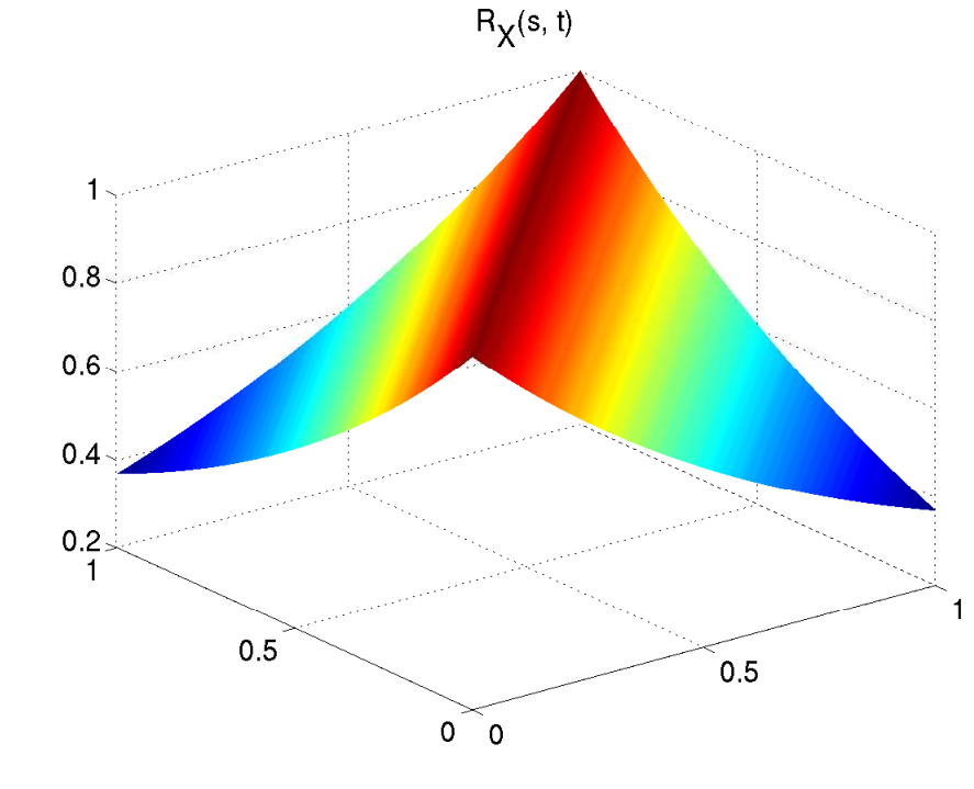
Here we consider the KL decomposition of a Gaussian random field $X$, which is characterized by its variance $\sigma^{2}$ and an autocorrelation function $R_{X}(s,t)$ given by,

We show in Figure 1(a) a plot of $R_{X}(s,t)$ over $[0,1]\times[0,1]$.

References

- [1] Roger G. Ghanem and Pol D. Spanos. Stochastic finite elements: a spectral approach. Springer-Verlag New York, Inc., New York, NY, USA, 1991.
- [2] Israel Gohberg, Seymour Goldberg, and M. A. Kaashoek. Basic classes of linear operators. 2004.
- [3] Olivier P. Le Maitre and Omar M. Knio. Spectral Methods for Uncertainty Quantification With Applications to Computational Fluid Dynamics. Scientific Computation. Springer, 2010.
- [4] Michel Loeve. Probability theory I, volume 45 of Graduate Texts in Mathematics. New York, Heidelberg, Berlin: Springer-Verlag, 1977.
- [5] Arch W. Naylor and George Sell. Linear operator theory in engineering and science. Springer-Verlag, New York, 1982.
- [6] L.C.G. Rogers and David Williams. Diffusions, Markov Processes, and Martingales: Volume 1, Foundations. Cambridge University Press, 2000.
- [7] L.C.G. Rogers and David Williams. Diffusions, Markov processes and martingales: Volume 2, Itô calculus. Cambridge university press, 2000.
- [8] Ralph C. Smith. Uncertainty Quantification: Theory, Implementation, and Applications, volume 12. SIAM, 2013.
- [9] David Williams. Probability with martingales. Cambridge Mathematical Textbooks. Cambridge University Press, Cambridge, 1991.
- [10] Dongbin Xiu. Numerical methods for stochastic computations: a spectral method approach. Princeton University Press, 2010.