Dark Photons from the Center of the Earth:
Smoking-Gun Signals of Dark Matter

Dark matter particles are captured when elastic scattering off nuclei $N$ in the Earth reduces their velocity below the escape velocity. The elastic scattering process $XN\to XN$ is mediated by $t$-channel $A^{\prime}$ exchange. The most relevant scattering targets, $N$, are iron and nickel; these and other elements are listed in Table 1. In the center-of-mass frame, the cross section is

where $E_{N}$, $Z_{N}$, $m_{N}$, and $F_{N}$ are the energy, electric charge, mass, and nuclear form factor of target nucleus $N$, and $\boldsymbol{p}$ is the center-of-mass 3-momentum of the dark matter. Since the collision is non-relativistic, $\boldsymbol{p}$ is negligible everywhere in Eq. (7), except possibly the denominator. The cross section may then be simplified to

where $\mu_{N}\equiv m_{N}m_{X}/(m_{N}+m_{X})$ is the reduced mass of the $X$–$N$ system.

It is tempting to simplify the denominator by neglecting $\boldsymbol{p}$, and reducing the $A^{\prime}$ exchange to a contact interaction. However, it is not always true that $m_{A^{\prime}}^{2}\gg\boldsymbol{p}^{2}$ so that the latter term may be neglected. The typical size of the momentum is $\boldsymbol{p}^{2}\sim\mu_{N}^{2}w^{2}$, where $w$ is the $X$ velocity in the lab frame. Since capture typically occurs only for very small asymptotic dark matter velocities, a reasonable choice would be $w=v_{\oplus}(r_{N})\approx 5\times 10^{-5}$, the escape velocity at the radius $r_{N}$ that maximizes the radial number density $n_{N}(r)r^{2}$ of target nucleus $N$. With these values, the contact interaction limit fails for $m_{A^{\prime}}\lesssim 3~\text{MeV}$. Rather than neglecting the momentum term altogether, a slightly more sophisticated approach would be to make the substitution $\boldsymbol{p}^{2}(1-\cos\theta_{\text{CM}})\to\mu_{N}^{2}w^{2}$. In this work, however, we keep the full $\boldsymbol{p}$ dependence in the propagator and evaluate the capture rate numerically so that our results are valid throughout parameter space. We have confirmed that our results reproduce those in the literature in the corners of parameter space where simplifying assumptions are valid. For example, they match Ref. [48] in the large-$m_{A^{\prime}}$, point-like cross section limit.

To determine capture rates, it is convenient to re-express the differential cross section as a function of recoil energy $E_{R}=\mu_{N}^{2}w^{2}(1-\cos\theta_{\text{CM}})/m_{N}$ in the lab frame. In the non-relativistic limit the expression simplifies to [49]

For $F_{N}$, we adopt the Helm form factor [50],

where $E_{N}\equiv 0.114~\text{GeV}/A_{N}^{5/3}$ is a characteristic energy scale for a target nucleus with atomic mass number $A_{N}$.

From this fundamental cross section we can determine the capture rate. The differential rate of dark matter particles scattering off nuclei with incident velocity $w$ at radius $r$ from the center of the Earth and imparting recoil energy between $E_{R}$ and $E_{R}+dE_{R}$ is given by

where $n_{X}=(0.3\text{ GeV}/\text{cm}^{3})/m_{X}$ and $n_{N}(r)$ are the dark matter and target nucleus number densities, respectively, and $f_{\oplus}(w,r)$ is the velocity distribution of incident dark matter at radius $r$, which is distorted from the free-space Maxwell–Boltzmann distribution, $f(u)$, by the Earth’s motion and gravitational potential. We follow the velocity notation introduced by Gould [13, 14, 16] where $v_{\oplus}(r)$ is the escape velocity at radius $r$ and $u$ is the dark matter velocity asymptotically far from the Earth.

The total capture rate is obtained by integrating Eq. (11) over the region of parameter space where the final state dark matter particle has energy less than $m_{X}v_{\oplus}^{2}(r)/2$ and is thus gravitationally captured. The escape velocity $v_{\oplus}(r)$ and number densities $n_{N}(r)$ are determined straightforwardly from the density data enumerated in the Preliminary Reference Earth Model [51]. Following Edsjö and Lundberg [20], the target number densities are modeled by dividing the Earth into two layers, the core and the mantle, with constant densities and elemental compositions given in Table 1. The capture rate is then $C_{\text{cap}}=\sum_{N}C_{\text{cap}}^{N}$, where the rate on target $N$ is

Here $\Theta(\Delta E)=\Theta(E_{\text{max}}-E_{\text{min}})$ imposes the constraint that capture is kinematically possible by enforcing that the minimum energy transfer, $E_{\text{min}}$, to gravitationally capture the dark matter particle is smaller than the maximum recoil energy kinematically allowed, $E_{\text{max}}$, corresponding to $\cos\theta_{\text{CM}}=-1$. Explicitly, these energies are

To make further progress, we must determine the distribution $f_{\oplus}(w,r)$. A simple approach is to only include the effect of the Earth’s gravitational potential. However, the Earth is within the gravitational influence of the Sun, and one might expect the acceleration of dark matter by the sun to suppress or eliminate the capture of heavy dark matter particles by the Earth. In 1991, however, Gould argued that the interactions of dark matter with other planets leads to diffusion of the dark matter population between bound and unbound orbits and one could thus ignore the impact of the Sun’s gravitational field and treat the Earth in the “free-space” approximation to reasonable accuracy [53].

More recently, however, this simple picture has been refined with both potentially positive and negative implications. In numerical work, both Lundberg and Edsjö [20] and Peter [21, 22, 23] have investigated the influence of the Sun, Earth, Jupiter, and Venus in more detail, tracking the possibility that the Earth’s dark matter population is suppressed when particles are kicked out of the solar system or captured by the Sun. For the case of supersymmetric WIMPs—that is, dark matter with weak-scale mediators—they have found that these effects can reduce the Earth’s capture rate by one order of magnitude or more, depending on the dark matter mass. On the other hand, simulations of galaxies with baryons have shown that dark matter substructures may be pulled into the disk and create a significant and relatively cold enhancement of the local dark matter density known as a “dark disk” [54, 55]. For the case of WIMP dark matter, this population may enhance indirect detection signals from the Earth by up to three orders of magnitude [24, 56]. Note that the dark disk has a velocity relative to our solar system that is $\sim 1/5$ that of the ordinary dark matter halo [57]. It is thus plausible that the dark disk populates a region in phase space more amenable to Earth capture without significantly enhancing the direct detection rate.

As we show below, the dark photon case differs significantly from WIMPs, because both the capture and annihilation rates are highly velocity dependent. One consequence of this is that $\tau_{\oplus}$ is typically larger than $\tau$ in Eq. (6), as opposed to the conventional wisdom that the Earth has not reached its WIMP capacity. It is therefore not possible to simply extrapolate the conclusions of WIMP studies to the present framework. In addition, as our analysis is valid for general dark matter and dark photon masses, inaccuracies in the particle physics modeling are greatly reduced, and the astrophysical uncertainties from dark disk and other effects are very likely the dominant uncertainties entering the signal rate derivation. These astrophysical phenomena are therefore clearly interesting and important, but are beyond the scope of the present work. Here, we use the free-space approximation, not because it is the last word, but because it provides a simple “middle ground” estimate, with both suppressions and enhancements possible.

With the free-space assumption, we proceed as follows. By energy conservation, $w$ and $u$, the incident dark matter particle’s velocities in the Earth’s and galactic frame, respectively, are related by

The capture rate for a general $d\sigma_{N}/dE_{R}$ can then be rewritten as

Here $f_{\oplus}(u)$ is defined to be the angular-averaged and annual-averaged velocity distribution in the rest frame of the Earth [58],

where $V_{\odot}\simeq 220~\text{km}/\text{s}$ is the velocity of the Sun relative to the galactic center, $V_{\oplus}\simeq 29.8~\text{km}/\text{s}$ is the velocity of the Earth relative to the Sun, and $\cos\gamma\approx 0.51$ is the angle of inclination of the Earth’s orbital plane relative to the Sun’s orbit. Many-body simulations and other considerations suggest a dark matter velocity distribution in the galactic rest frame of the form [59, 60, 61, 62, 63, 64]

where $N_{0}$ is a normalization constant, $v_{\text{gal}}$ is the escape velocity from the galaxy, and the parameters describing the distribution have typical values in the ranges [48, 65]

We use the midpoint values of each of these, namely, $u_{0}=245~\text{km}/\text{s}$, $v_{\text{gal}}=550~\text{km}/\text{s}$, and $k=2.5$. The truncated Maxwell–Boltzmann distribution is recovered for $k=0$.

Upon inserting Eq. (9), the $dE_{R}$ integral in Eq. (15) evaluates to

where we use the substitution variable $x_{N}$ and exponential integral function [66],

The total rate is $C_{\text{cap}}=\sum C_{\text{cap}}^{N}=32\pi^{3}\varepsilon^{2}\alpha_{X}\alpha n_{X}\sum_{N}Z_{N}^{2}(m_{N}E_{N})^{-1}\text{exp}\left(\frac{m_{A^{\prime}}^{2}}{2m_{N}E_{N}}\right)c_{\text{cap}}^{N}$, where

The capture rates $C_{\text{cap}}^{N}$ for various nuclei $N$ at a representative point in parameter space are shown in Table 1.

Once a dark matter particle is captured by the Earth, it repeatedly re-scatters, drops to the center of the Earth, and eventually thermalizes with the surrounding matter. In the case of the Sun, the dark matter thermalizes within the age of the Sun for $X$–proton spin-independent scattering cross sections greater than $10^{-51}$, $10^{-50}$, and $10^{-47}~\text{cm}^{2}$ for $m_{X}=100~\text{GeV}$, 1 TeV, and 10 TeV, respectively [23]. Similar studies of Earth capture are not available. However, we will find that, for the range of parameters where an observable indirect signal is possible, the direct detection $X$–proton cross sections are at least $\sigma_{p}\sim 10^{-48}~\text{cm}^{2}$, corresponding to $X$–iron cross sections of $\sigma_{\text{Fe}}\sim Z_{\text{Fe}}^{2}(m_{\text{Fe}}/m_{p})^{2}\sigma_{p}\sim 10^{-42}~\text{cm}^{2}$, many orders of magnitude larger than required for thermalization in the Sun. We therefore expect dark matter to be thermalized in the Earth to an excellent approximation.

For thermalized dark matter, the annihilation rate parameter $C_{\text{ann}}$ is [48]

where $\rho_{\oplus}\approx 13~\text{g}/\text{cm}^{3}$ and $T_{\oplus}\approx 5700~\text{K}$ are the matter density and temperature at the center of the Earth, respectively, $\sigma_{\text{ann}}$ is the cross section for $XX\to A^{\prime}A^{\prime}$, and $v$ is the relative velocity of the interacting particles, which is double the velocity of either interacting particle in the center-of-mass frame.

The thermally-averaged cross section is

where

is the tree-level cross section [67], and $\langle S_{S}\rangle$ is the thermal average of the $S$-wave Sommerfeld enhancement factor. This Sommerfeld enhancement factor [68] has been determined with various degrees of refinement. An analytic expression that includes the resonance behavior present for non-zero $m_{A^{\prime}}$ can be derived by approximating the Yukawa potential by the Hulthén potential [69, 70, 71]. The resulting Sommerfeld factor is

where $a=v/(2\alpha_{X})$ and $c=6\alpha_{X}m_{X}/(\pi^{2}m_{A^{\prime}})$. The thermal average is, then,

where $v_{0}=\sqrt{2T_{\oplus}/m_{X}}$.

In Fig. 2 we present results for the equilibrium timescale $\tau=(C_{\text{cap}}C_{\text{ann}})^{-1/2}$ in the $(m_{A^{\prime}},\varepsilon)$ plane for $m_{X}=100~\text{GeV}$ without Sommerfeld enhancement, and $m_{X}=100~\text{GeV},1~\text{TeV},10~\text{TeV}$ with Sommerfeld enhancement. The dark coupling $\alpha_{X}$ is fixed by the thermal relic density. For $m_{A^{\prime}}\ll m_{X}$, the parametric dependence of $\tau$ on $\varepsilon$ and $m_{A^{\prime}}$ enters dominantly through $C_{\text{ann}}$ and is $\tau\sim C_{\text{ann}}^{-1/2}\sim m_{A^{\prime}}^{2}/\varepsilon$. This can be seen in the baseline values of the contours in Fig. 2. The bumps in the contours reflect the resonance structure of the Sommerfeld enhancement factor $\langle S_{S}\rangle$.

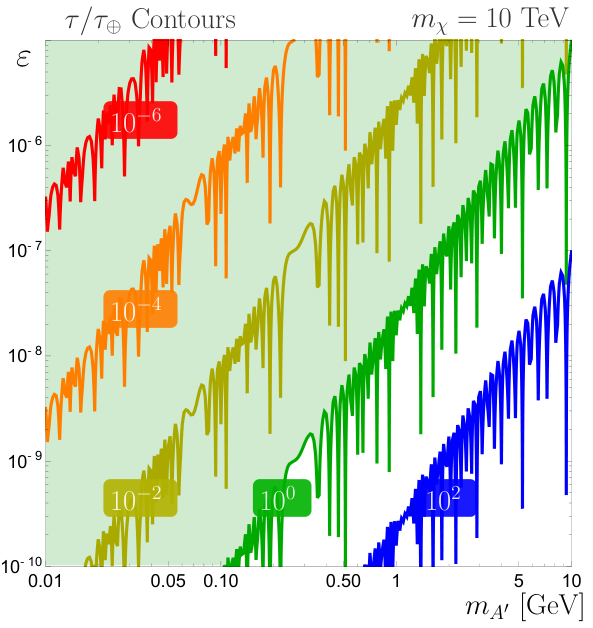
In the shaded green (upper left) parts of the figures, the Earth’s dark matter population has reached its maximal (equilibrium) value, and so the annihilation rate is essentially determined by the capture rate, with $\Gamma_{\text{ann}}\approx\frac{1}{2}C_{\text{cap}}$. As one moves down and to the right, however, the equilibrium timescale grows, and the population is eventually not maximal. We will see that when the population is not at its maximal value, the signal quickly becomes undetectable.

The Sommerfeld enhancement plays an essential role in reducing the equilibrium timescale and making the signal detectable in large regions of the $(m_{A^{\prime}},\varepsilon)$ plane. For capture, the typical velocity that enters has an irreducible contribution from the gravitational potential that accelerates dark matter as it falls into the Earth. Capture interactions, therefore, occur at the typical escape velocity in the Earth’s core, $v_{\text{esc}}\approx 5.0\times 10^{-5}$. However, after the dark matter particles are captured, they sink to the core, and come into thermal equilibrium with the normal matter. As a result, the population of dark matter particles at the center of the Earth is even colder, with relative velocities $v_{0}\approx 1.0\times 10^{-6}\,[\text{TeV}/m_{X}]^{1/2}$. In the $m_{A^{\prime}}\ll\alpha_{X}m_{X}$ limit, the Sommerfeld factor of Eq. (25) becomes

For thermal relics, $S_{0}$ is therefore typically $\sim 2\pi\alpha_{X}/v\sim 10^{4}-10^{6}$. Sommerfeld enhancement therefore reduces the equilibrium timescale by factors of $\sim 100$ for $m_{X}\sim 100~\text{GeV}$, as can be seen in Fig. 2 by comparing the top right and top left panels. This reduction on $\tau$ goes to $\sim 1000$ for $m_{X}\sim 10~\text{TeV}$. The Sommerfeld factor therefore plays an essential role in boosting the current Earth’s dark matter population and the dark matter signal [26].

Dark photons may be detected in IceCube if they decay in IceCube or just below it. Decays $A^{\prime}\to e^{+}e^{-},q\bar{q}$ will be seen as showers, and for $m_{A^{\prime}}\gtrsim 300~\text{MeV}$, typically 15% – 40% of the decays will be to muons [46] and be seen as tracks. The number of dark photon decays that can be detected by IceCube is

where the factor of 2 results from the fact that each annihilation produces two dark photons, $A_{\text{eff}}$ is the effective area of detector,

is the probability that the dark photon decays after traveling a distance between $R_{\oplus}$ and $R_{\oplus}+D$, where $D$ is the effective depth of the detector, and $T$ is the live time of the experiment.

To very roughly estimate the detection rates for IceCube, we expect that for $m_{X}\sim 1~\text{TeV}$, all dark photons that decay within the instrumented volume of IceCube are detected, and so we take $A_{\text{eff}}\approx 1~\text{km}^{2}$ and $D\approx 1~\text{km}$. For lighter dark matter, say, $m_{X}\sim 100~\text{GeV}$, the decay products may be lost between the photomultiplier strings of IceCube. But these should be seen with high efficiency in DeepCore [72], the subset of IceCube with finer string spacings and lower threshold, and so we also present results for the instrumented volume of DeepCore, with $A_{\text{eff}}\approx 0.067~\text{km}^{2}$ and $D\approx 0.55~\text{km}$.

In Fig. 3 we present the number of signal events for $m_{X}=100~\text{GeV}$, 1 TeV, and 10 TeV in the $(m_{A^{\prime}},\varepsilon)$ plane. The bumpy features and closed contours are real physical features resulting from Sommerfeld enhancement resonances. Also shown are the regions of parameter space disfavored by existing bounds on dark-photon-mediated $XN\to XN$ scattering from direct detection experiments, such as PANDAX-II [73, 78], and $X$-independent bounds on dark photons from beam dump experiments and supernovae [74, 75, 5, 76, 77, 79]. We use the recently updated supernova cooling bounds in Ref. [79].

We see that the indirect detection signal discussed here probes regions of parameter space that are so far inaccessible by other methods. As anticipated in Sec. II, the indirect detection signal is largest for $\varepsilon\sim 10^{-10}-10^{-8}$, where the $A^{\prime}$ decay length is comparable to $R_{\oplus}$. For $m_{X}\sim 10~\text{TeV}$ and $\varepsilon\sim 10^{-8}$, for example, $N_{\text{sig}}\sim 1,000$ events over 10 years are possible in regions of parameter space that are otherwise currently viable. IceCube has collected roughly 7 years of data already, and so detailed analyses will either exclude large new regions of the $(m_{A^{\prime}},\varepsilon)$ parameter space or discover dark matter.

For $m_{X}\sim 100~\text{GeV}$, the indirect and direct detection sensitivities are comparable for $\alpha_{X}$ between $\alpha_{X}^{\text{th}}$ and $\alpha_{X}^{\text{max}}$. The indirect and direct detection sensitivities are shown in the conventional $(m_{X},\sigma_{Xn})$ plane in Fig. 4, where $\sigma_{Xn}$ is the spin-independent $X$–nucleon cross section: $\mu_{T}^{2}A_{T}^{2}\sigma_{Xn}=\mu_{n}^{2}\sigma_{XT}$ with $T=\text{Xe}$. The indirect detection signal is suppressed for both large $\sigma_{Xn}$ (large $\varepsilon$, dark photons decay too soon) and small $\sigma_{Xn}$ (small $\varepsilon$, dark matter capture is too slow and the captive population does not equilibrate). Of course, the large $\sigma_{Xn}$ are already excluded by direct detection experiments. Focusing on the small $\sigma_{Xn}$ region, for $m_{X}>100~\text{GeV}$, the indirect detection signals probe cross sections as much as three orders of magnitude below the current bounds from direct detection experiments, such as XENON and LUX.

Since $\sigma_{Xn}\sim\alpha_{X}\varepsilon^{2}$, a given $\sigma_{Xn}$ corresponds to a larger value of $\varepsilon$ when assuming the thermal $\alpha_{X}^{\text{th}}$ versus maximal $\alpha_{X}^{\text{max}}$ dark sector coupling. For this reason, the dashed $\alpha_{X}^{\text{max}}$ curves on the left-hand plot in Fig. 4 are sometimes above the solid $\alpha_{X}^{\text{th}}$ curves on the $(m_{X},\sigma_{Xn})$ plane. This is because when going from $\alpha_{X}^{\text{th}}$ to $\alpha_{X}^{\text{max}}$, the additional $\varepsilon$ reach gained in indirect detection experiments is less than that in direct detection experiments. The reason for this is straightforward: the lower bound on the IceCube reach is set by the condition that the $\tanh^{2}(\tau_{\oplus}/\tau)$ in Eq. (6) is ‘saturated’ near unity, i.e. that dark matter capture and annihilation are in equilibrium. This is why the lower contours of Fig. 3 display the same resonances as Fig. 2. Since this condition is set by the geometric mean of the capture and annihilation rates, it scales differently from direct detection experiments which has the same parametric dependence as the capture rate.

The detector’s effective area $A_{\text{eff}}$ and depth $D$ are, of course, dependent on the energy and type of the dark photon decay products, and a more detailed study of detector response is required to estimate these more accurately. This is beyond the scope of the present work, but we note here some basic considerations. Muons with energies $E_{\mu}\sim 100~\text{GeV}-\text{TeV}$ lose energy primarily through ionization and travel a distance

before their energy drops below a threshold energy $E_{\text{th}}$, where $\rho=1~\text{g}/\text{cm}^{3}$, $\alpha\simeq 2.0~\text{MeV}~\text{cm}^{2}/\text{g}$, and $\beta\simeq 4.2\times 10^{-6}~\text{cm}^{2}/\text{g}$ [84]. For $E_{\mu}=1~\text{TeV}$ and $E_{\text{th}}=50~\text{GeV}$, on average muons travel a distance $L_{\mu}=2.5~\text{km}$. Dark photons that decay to muons a km or two below IceCube may therefore be detected in IceCube, and so the effective depth of IceCube is a bit larger than 1 km. For $m_{X}\sim 10~\text{TeV}$, the effective depth is larger still, although less than a naive application of Eq. (32) would indicate, as such high energy muons lose energy primarily through radiative processes. At TeV energies, the experimental angular resolution for muon tracks is less than a degree, providing a powerful handle to reduce background. For the case of showers from electrons or hadrons, the angular resolution is worse, but still sufficient to identify showers as up-going to within tens of degrees. In addition, because dark photons decay completely to visible particles, contained events are mono-energetic, with the total energy equal to $m_{X}$. The angle and energy distributions of tracks and showers are therefore completely different from astrophysical sources, and provide powerful handles for differentiating signal from background.

The dark photon signal has two primaries, which could in principle be identified as a smoking-gun signal for the dark sector. In Figs. 5 and 6 we show histograms of the velocity difference (time delay) and opening angle (track separation) of the two muons produced in a dark photon decay. Details of the distributions are presented in the Appendix. Parallel tracks have been considered previously in the context of slepton production from high energy neutrinos in Refs. [85, 86] and have recently been searched for by IceCube [87]. As a benchmark for IceCube reach, the parameters $m_{X}=1~\text{TeV}$, $m_{A^{\prime}}=500~\text{MeV}$, and $\varepsilon=5\times 10^{-9}$ gives an expected 40 muon events in 10 live years. The center panels of Figs. 5 and 6 then show that over $\sim 2.5~\text{km}$ between the $A^{\prime}$ decay point and the maximal detection distance, one expects a few events with timing separation of $\sim 0.03$ ns and $\sim 20$ m track separation.

The timing separation is below the IceCube Digital Optical Module timing resolution of $\sim 5$ ns [88]. The track separations are less than the $\sim 100~\text{m}$ separations probed by current analyses [87], but they are also much larger than the $\sim 1~\text{m}$ separations from SM neutrino-induced charm production. These results motivate looking for parallel muon tracks with ${\cal O}(10~\text{m})$ separations, which would be an unambiguous signal of physics beyond the SM, and a spectacular signal of dark photons and dark matter. One step in this direction is the proposed PINGU upgrade which would densely instrument a subset of the IceCube/DeepCore detector [89]. However, for the proposed dark photon search, this comes at a large cost in available volume and propagation distance. A possible alternative direction to improve sensitivity to these parallel muon signals is to increase the detector density of the IceTop surface array.

The dark photon decay products may also be detected by space-based cosmic ray detectors, such as Fermi-LAT and AMS-02. Though these are far smaller than IceCube, the dark photon may decay anywhere between the Earth’s surface and the detector, providing a partially-compensating enhancement to the rate. For Fermi and AMS, we follow the formalism described above, but now use $A_{\text{eff}}=1~\text{m}^{2}$. Both Fermi and AMS are in low Earth orbit, flying 550 and 400 km above the ground, respectively. We choose $D=550~\text{km}$ in Eq. (31). Note that, after the dark photon decays, the resulting charged particles are bent in the Earth’s magnetic field by an angle

where $p$ is the particle’s momentum, $L$ is the distance it travels, and we have normalized the Earth’s magnetic field $B$ to an average value at the surface of the Earth. For $m_{X}\gtrsim\text{TeV}$, this deflection is less than the dispersion from the dark matter’s spatial distribution at the center of the Earth given in Eq. (28), but for $m_{X}\sim 100~\text{GeV}$, this deflection may be significant, and the signal may arrive at an angle as large as $5^{\circ}$ relative to straight down.

The resulting event rates for such space-based detectors are given in Fig. 7 for a live time of 10 years. The parameter space that can be probed largely overlaps with that already probed by direct detection, but Fermi and AMS may set bounds complementary to the existing direct detection experiments. As a benchmark, consider the parameters $m_{X}=1~\text{TeV}$, $m_{A^{\prime}}=400~\text{MeV}$, and $\varepsilon=10^{-8}$, for which one expects $N_{\text{sig}}=10$ signal events in 10 live years. The velocity difference and opening angle distributions are shown in the center panels of Figs. 5 and 6. For a primary propagation distance of $\sim 300~\text{km}$, this yields timing separations of up to tens of nanoseconds and separations of up to a kilometer. We therefore do not expect to see both primary particles from dark photon decay in Fermi or AMS. Of course, this is still possible: the $A^{\prime}$ may decay near Fermi or AMS; secondary photons from hadronic final states my happen to have little transverse momentum; or the $A^{\prime}$ may decay far from the detectors to two charged particles, which are both bent by the magnetic field into the detectors. Although possible, all of these are highly improbable, and two-particle events are a small fraction of the total number of single-particle signal events. An alternative possibility is when there is a small splitting between $m_{A^{\prime}}$ and $2m_{f}$. In this case the decay products have small transverse momentum by Eq. (29), at the cost of a reduced branching ratio.

Last, the number of signal events $N_{\text{sig}}$ does not take into account experimental efficiencies associated with each apparatus. For example, we have assumed that the volume of the International Space Station between the Earth and AMS does not affect the dark photon primaries, and, further, that the hadronic products of the dark photons are detectable. A more complete analysis of the Fermi/AMS reach will require more realistic modeling and different triggers.

References

- [1] I. Y. Kobzarev, L. Okun, and I. Y. Pomeranchuk, “On the possibility of experimental observation of mirror particles,” Sov.J.Nucl.Phys. 3 (1966) 837–841.
- [2] L. B. Okun, “Limits of Electrodynamics: Paraphotons?,” Sov. Phys. JETP 56 (1982) 502. [Zh. Eksp. Teor. Fiz.83,892(1982)].
- [3] B. Holdom, “Two U(1)’s and Epsilon Charge Shifts,” Phys.Lett. B166 (1986) 196.
- [4] B. Holdom, “Searching for Charges and a New U(1),” Phys. Lett. B178 (1986) 65.
- [5] R. Essig et al., “Working Group Report: New Light Weakly Coupled Particles,” in Community Summer Study 2013: Snowmass on the Mississippi (CSS2013) Minneapolis, MN, USA, July 29-August 6, 2013. 2013. arXiv:1311.0029 [hep-ph].
- [6] R. Foot, “Mirror dark matter: Cosmology, galaxy structure and direct detection,” Int.J.Mod.Phys. A29 (2014) 1430013, arXiv:1401.3965 [astro-ph.CO].
- [7] K. Freese, “Can Scalar Neutrinos Or Massive Dirac Neutrinos Be the Missing Mass?,” Phys. Lett. B167 (1986) 295.
- [8] W. H. Press and D. N. Spergel, “Capture by the Sun of a Galactic Population of Weakly Interacting Massive Particles,” Astrophys.J. 296 (1985) 679–684.
- [9] J. Silk, K. A. Olive, and M. Srednicki, “The Photino, the Sun and High-Energy Neutrinos,” Phys. Rev. Lett. 55 (1985) 257–259.
- [10] L. M. Krauss, M. Srednicki, and F. Wilczek, “Solar System Constraints and Signatures for Dark Matter Candidates,” Phys. Rev. D33 (1986) 2079–2083.
- [11] K. Griest and D. Seckel, “Cosmic Asymmetry, Neutrinos and the Sun,” Nucl.Phys. B283 (1987) 681.
- [12] T. K. Gaisser, G. Steigman, and S. Tilav, “Limits on Cold Dark Matter Candidates from Deep Underground Detectors,” Phys. Rev. D34 (1986) 2206.
- [13] A. Gould, “WIMP Distribution in and Evaporation From the Sun,” Astrophys.J. 321 (1987) 560.
- [14] A. Gould, “Resonant Enhancements in WIMP Capture by the Earth,” Astrophys.J. 321 (1987) 571.
- [15] A. Gould, “Direct and indirect capture of weakly interacting massive particles by the earth,”Astrophys. J. 328 (May, 1988) 919–939.
- [16] A. Gould, “Cosmological density of WIMPs from solar and terrestrial annihilations,” Astrophys.J. 388 (1992) 338–344.
- [17] T. Damour and L. M. Krauss, “A New solar system population of WIMP dark matter,” Phys. Rev. Lett. 81 (1998) 5726–5729, arXiv:astro-ph/9806165 [astro-ph].
- [18] T. Damour and L. M. Krauss, “A New WIMP population in the solar system and new signals for dark matter detectors,” Phys. Rev. D59 (1999) 063509, arXiv:astro-ph/9807099 [astro-ph].
- [19] A. Gould and S. M. Khairul Alam, “Can heavy WIMPs be captured by the earth?,” Astrophys. J. 549 (2001) 72–75, arXiv:astro-ph/9911288 [astro-ph].
- [20] J. Lundberg and J. Edsjo, “WIMP diffusion in the solar system including solar depletion and its effect on earth capture rates,” Phys. Rev. D69 (2004) 123505, arXiv:astro-ph/0401113 [astro-ph].
- [21] A. H. G. Peter, “Dark matter in the solar system I: The distribution function of WIMPs at the Earth from solar capture,” Phys. Rev. D79 (2009) 103531, arXiv:0902.1344 [astro-ph.HE].
- [22] A. H. G. Peter, “Dark matter in the solar system II: WIMP annihilation rates in the Sun,” Phys. Rev. D79 (2009) 103532, arXiv:0902.1347 [astro-ph.HE].
- [23] A. H. G. Peter, “Dark matter in the solar system III: The distribution function of WIMPs at the Earth from gravitational capture,” Phys. Rev. D79 (2009) 103533, arXiv:0902.1348 [astro-ph.HE].
- [24] T. Bruch, A. H. G. Peter, J. Read, L. Baudis, and G. Lake, “Dark Matter Disc Enhanced Neutrino Fluxes from the Sun and Earth,” Phys. Lett. B674 (2009) 250–256, arXiv:0902.4001 [astro-ph.HE].
- [25] S. M. Koushiappas and M. Kamionkowski, “Galactic Substructure and Energetic Neutrinos from the Sun and the Earth,” Phys. Rev. Lett. 103 (2009) 121301, arXiv:0907.4778 [astro-ph.CO].
- [26] C. Delaunay, P. J. Fox, and G. Perez, “Probing Dark Matter Dynamics via Earthborn Neutrinos at IceCube,” JHEP 05 (2009) 099, arXiv:0812.3331 [hep-ph].
- [27] P. Schuster, N. Toro, and I. Yavin, “Terrestrial and Solar Limits on Long-Lived Particles in a Dark Sector,” Phys. Rev. D81 (2010) 016002, arXiv:0910.1602 [hep-ph].
- [28] P. Schuster, N. Toro, N. Weiner, and I. Yavin, “High Energy Electron Signals from Dark Matter Annihilation in the Sun,” Phys. Rev. D82 (2010) 115012, arXiv:0910.1839 [hep-ph].
- [29] P. Meade, S. Nussinov, M. Papucci, and T. Volansky, “Searches for Long Lived Neutral Particles,” JHEP 06 (2010) 029, arXiv:0910.4160 [hep-ph].
- [30] B. Batell, M. Pospelov, A. Ritz, and Y. Shang, “Solar Gamma Rays Powered by Secluded Dark Matter,” Phys. Rev. D81 (2010) 075004, arXiv:0910.1567 [hep-ph].
- [31] The Fermi LAT Collaboration, M. Ajello et al., “Constraints on Dark Matter Models from a Fermi Lat Search for High-Energy Cosmic-Ray Electrons from the Sun,” Phys. Rev. D84 (2011) 032007, arXiv:1107.4272 [astro-ph.HE].
- [32] I. F. M. Albuquerque, C. Perez de Los Heros, and D. S. Robertson, “Constraints on self interacting dark matter from IceCube results,” JCAP 1402 (2014) 047, arXiv:1312.0797 [astro-ph.CO].
- [33] J. Chen, Z.-L. Liang, Y.-L. Wu, and Y.-F. Zhou, “Long-Range Self-Interacting Dark Matter in the Sun,” arXiv:1505.04031 [hep-ph].
- [34] J. Berger, Y. Cui, and Y. Zhao, “Detecting Boosted Dark Matter from the Sun with Large Volume Neutrino Detectors,” JCAP 1502 (2015) 005, arXiv:1410.2246 [hep-ph].
- [35] M. Vogelsberger, J. Zavala, and A. Loeb, “Subhaloes in Self-Interacting Galactic Dark Matter Haloes,” Mon. Not. R. Astron. Soc. 423 (2012) 3740, arXiv:1201.5892 [astro-ph.CO].
- [36] M. Rocha, A. H. G. Peter, J. S. Bullock, M. Kaplinghat, S. Garrison-Kimmel, J. Onorbe, and L. A. Moustakas, “Cosmological Simulations with Self-Interacting Dark Matter I: Constant Density Cores and Substructure,” Mon. Not. R. Astron. Soc. 430 (2013) 81–104, arXiv:1208.3025 [astro-ph.CO].
- [37] A. H. G. Peter, M. Rocha, J. S. Bullock, and M. Kaplinghat, “Cosmological Simulations with Self-Interacting Dark Matter Ii: Halo Shapes Vs. Observations,” Mon. Not. R. Astron. Soc. 430 (2013) 105, arXiv:1208.3026 [astro-ph.CO].
- [38] J. Zavala, M. Vogelsberger, and M. G. Walker, “Constraining Self-Interacting Dark Matter with the Milky Way’s Dwarf Spheroidals,” Mon. Not. R. Astro. Soc. 431 (2013) L20–L24, arXiv:1211.6426 [astro-ph.CO].
- [39] S. Tulin, H.-B. Yu, and K. M. Zurek, “Beyond Collisionless Dark Matter: Particle Physics Dynamics for Dark Matter Halo Structure,” Phys. Rev. D87 (2013) 115007, arXiv:1302.3898 [hep-ph].
- [40] M. Collie and R. Foot, “Neutrino masses in the SU(5) x SU(5)-prime mirror symmetric model,” Phys.Lett. B432 (1998) 134–138, arXiv:hep-ph/9803261 [hep-ph].
- [41] M. Kaplinghat, T. Linden, and H.-B. Yu, “Galactic Center Excess in Rays from Annihilation of Self-Interacting Dark Matter,” Phys. Rev. Lett. 114 (2015) 211303, arXiv:1501.03507 [hep-ph].
- [42] J. A. Adams, S. Sarkar, and D. W. Sciama, “CMB anisotropy in the decaying neutrino cosmology,” Mon. Not. Roy. Astron. Soc. 301 (1998) 210–214, arXiv:astro-ph/9805108 [astro-ph].
- [43] X.-L. Chen and M. Kamionkowski, “Particle decays during the cosmic dark ages,” Phys. Rev. D70 (2004) 043502, arXiv:astro-ph/0310473 [astro-ph].
- [44] N. Padmanabhan and D. P. Finkbeiner, “Detecting dark matter annihilation with CMB polarization: Signatures and experimental prospects,” Phys. Rev. D72 (2005) 023508, arXiv:astro-ph/0503486 [astro-ph].
- [45] T. R. Slatyer, “Indirect Dark Matter Signatures in the Cosmic Dark Ages I. Generalizing the Bound on s-wave Dark Matter Annihilation from Planck,” arXiv:1506.03811 [hep-ph].
- [46] M. Buschmann, J. Kopp, J. Liu, and P. A. N. Machado, “Lepton Jets from Radiating Dark Matter,” JHEP 07 (2015) 045, arXiv:1505.07459 [hep-ph].
- [47] A. R. Zentner, “High-Energy Neutrinos From Dark Matter Particle Self-Capture Within the Sun,” Phys. Rev. D80 (2009) 063501, arXiv:0907.3448 [astro-ph.HE].
- [48] P. Baratella, M. Cirelli, A. Hektor, J. Pata, M. Piibeleht, et al., “PPPC 4 DM : a Poor Particle Physicist Cookbook for Neutrinos from Dark Matter Annihilations in the Sun,” JCAP 1403 (2014) 053, arXiv:1312.6408 [hep-ph].
- [49] N. Fornengo, P. Panci, and M. Regis, “Long-Range Forces in Direct Dark Matter Searches,” Phys. Rev. D84 (2011) 115002, arXiv:1108.4661 [hep-ph].
- [50] J. Lewin and P. Smith, “Review of Mathematics, Numerical Factors, and Corrections for Dark Matter Experiments Based on Elastic Nuclear Recoil,” Astropart.Phys. 6 (1996) 87–112.
- [51] A. M. Dziewonski and D. L. Anderson, “Preliminary reference Earth model,” Physics of The Earth and Planetary Interiors 25 (1981) 297–356.
- [52] H. D. Holland and K. K. Turekian, Treatise on Geochemistry. Pergamon [Imprint], 2003.
- [53] A. Gould, “Gravitational diffusion of solar system WIMPs,” ApJ 368 (1991) 610–615.
- [54] J. I. Read, L. Mayer, A. M. Brooks, F. Governato, and G. Lake, “A dark matter disc in three cosmological simulations of Milky Way mass galaxies,” Mon. Not. R. Astro. Soc. 397 (2009) 44–51, arXiv:0902.0009.
- [55] J. I. Read, G. Lake, O. Agertz, and V. P. Debattista, “Thin, thick and dark discs in CDM,” Mon. Not. R. Astro. Soc. 389 (2008) 1041–1057, arXiv:0803.2714.
- [56] C. W. Purcell, J. S. Bullock, and M. Kaplinghat, “The Dark Disk of the Milky Way,” Astrophys. J. 703 (2009) 2275–2284, arXiv:0906.5348 [astro-ph.GA].
- [57] A. Peter, “Dark Matter Bound to the Solar System: Consequences for Annihilation Searches,” in Proceedings, 44Th Rencontres De Moriond on Electroweak Interactions and Unified Theories, pp. 359–366. 2009. arXiv:0905.2456 [astro-ph.HE].
- [58] J. D. Vergados, “Modulation effect in the differential rate for supersymmetric dark matter detection,” Phys. Rev. D58 (1998) 103001, arXiv:hep-ph/9802253 [hep-ph].
- [59] M. Vogelsberger, A. Helmi, V. Springel, S. D. White, J. Wang, et al., “Phase-Space Structure in the Local Dark Matter Distribution and Its Signature in Direct Detection Experiments,” Mon. Not. R. Astron. Soc. 395 (2009) 797–811, arXiv:0812.0362 [astro-ph].
- [60] M. Fairbairn and T. Schwetz, “Spin-Independent Elastic WIMP Scattering and the Dama Annual Modulation Signal,” JCAP 0901 (2009) 037, arXiv:0808.0704 [hep-ph].
- [61] M. Kuhlen, N. Weiner, J. Diemand, P. Madau, B. Moore, et al., “Dark Matter Direct Detection with Non-Maxwellian Velocity Structure,” JCAP 1002 (2010) 030, arXiv:0912.2358 [astro-ph.GA].
- [62] F. Ling, E. Nezri, E. Athanassoula, and R. Teyssier, “Dark Matter Direct Detection Signals Inferred from a Cosmological N-Body Simulation with Baryons,” JCAP 1002 (2010) 012, arXiv:0909.2028 [astro-ph.GA].
- [63] M. Lisanti, L. E. Strigari, J. G. Wacker, and R. H. Wechsler, “The Dark Matter at the End of the Galaxy,” Phys. Rev. D83 (2011) 023519, arXiv:1010.4300 [astro-ph.CO].
- [64] Y.-Y. Mao, L. E. Strigari, R. H. Wechsler, H.-Y. Wu, and O. Hahn, “Halo-To-Halo Similarity and Scatter in the Velocity Distribution of Dark Matter,” Astrophys.J. 764 (2013) 35, arXiv:1210.2721 [astro-ph.CO].
- [65] K. Choi, C. Rott, and Y. Itow, “Impact of the Dark Matter Velocity Distribution on Capture Rates in the Sun,” JCAP 1405 (2014) 049, arXiv:1312.0273 [astro-ph.HE].
- [66] M. Abramowitz and I. Stegun, Handbook of Mathematical Functions: With Formulas, Graphs, and Mathematical Tables. Applied mathematics series. Dover Publications, 1964.
- [67] J. Liu, N. Weiner, and W. Xue, “Signals of a Light Dark Force in the Galactic Center,” JHEP 08 (2015) 050, arXiv:1412.1485 [hep-ph].
- [68] A. Sommerfeld, “Über die Beugung und Bremsung der Elektronen,” Ann. der Physik 403 (1931) 257.
- [69] S. Cassel, “Sommerfeld factor for arbitrary partial wave processes,” J.Phys. G37 (2010) 105009, arXiv:0903.5307 [hep-ph].
- [70] T. R. Slatyer, “The Sommerfeld enhancement for dark matter with an excited state,” JCAP 1002 (2010) 028, arXiv:0910.5713 [hep-ph].
- [71] J. L. Feng, M. Kaplinghat, and H.-B. Yu, “Sommerfeld Enhancements for Thermal Relic Dark Matter,” Phys. Rev. D82 (2010) 083525, arXiv:1005.4678 [hep-ph].
- [72] IceCube Collaboration, R. Abbasi et al., “The Design and Performance of IceCube DeepCore,” Astropart. Phys. 35 (2012) 615–624, arXiv:1109.6096 [astro-ph.IM].
- [73] E. Del Nobile, M. Kaplinghat, and H.-B. Yu, “Direct Detection Signatures of Self-Interacting Dark Matter with a Light Mediator,” arXiv:1507.04007 [hep-ph].
- [74] J. B. Dent, F. Ferrer, and L. M. Krauss, “Constraints on Light Hidden Sector Gauge Bosons from Supernova Cooling,” arXiv:1201.2683 [astro-ph.CO].
- [75] H. K. Dreiner, J.-F. Fortin, C. Hanhart, and L. Ubaldi, “Supernova constraints on MeV dark sectors from annihilations,” Phys. Rev. D89 (2014) 105015, arXiv:1310.3826 [hep-ph].
- [76] D. Kazanas, R. N. Mohapatra, S. Nussinov, V. L. Teplitz, and Y. Zhang, “Supernova Bounds on the Dark Photon Using its Electromagnetic Decay,” Nucl.Phys. B890 (2014) 17–29, arXiv:1410.0221 [hep-ph].
- [77] E. Rrapaj and S. Reddy, “Nucleon-nucleon bremsstrahlung of dark gauge bosons and revised supernova constraints,” arXiv:1511.09136 [nucl-th].
- [78] PandaX-II Collaboration, X. Cui et al., “Dark Matter Results From 54-Ton-Day Exposure of PandaX-II Experiment,” arXiv:1708.06917 [astro-ph.CO].
- [79] C. Mahoney, A. K. Leibovich, and A. R. Zentner, “Updated Constraints on Self-Interacting Dark Matter from Supernova 1987A,” Phys. Rev. D96 (2017) no. 4, 043018, arXiv:1706.08871 [hep-ph].
- [80] LUX Collaboration, D. S. Akerib et al., “First Results from the Lux Dark Matter Experiment at the Sanford Underground Research Facility,” Phys. Rev. Lett. 112 (2014) 091303, arXiv:1310.8214 [astro-ph.CO].
- [81] M. Kaplinghat, S. Tulin, and H.-B. Yu, “Direct Detection Portals for Self-interacting Dark Matter,” Phys. Rev. D89 (2014) 035009, arXiv:1310.7945 [hep-ph].
- [82] H. An, M. Pospelov, J. Pradler, and A. Ritz, “Direct Detection Constraints on Dark Photon Dark Matter,” Phys. Lett. B747 (2015) 331–338, arXiv:1412.8378 [hep-ph].
- [83] J. Billard, L. Strigari, and E. Figueroa-Feliciano, “Implication of Neutrino Backgrounds on the Reach of Next Generation Dark Matter Direct Detection Experiments,” Phys. Rev. D89 (2014) no. 2, 023524, arXiv:1307.5458 [hep-ph].
- [84] Particle Data Group Collaboration, K. A. Olive et al., “Review of Particle Physics,” Chin. Phys. C38 (2014) 090001.
- [85] I. Albuquerque, G. Burdman, and Z. Chacko, “Neutrino telescopes as a direct probe of supersymmetry breaking,” Phys. Rev. Lett. 92 (2004) 221802, arXiv:hep-ph/0312197 [hep-ph].
- [86] I. F. M. Albuquerque, G. Burdman, and Z. Chacko, “Direct detection of supersymmetric particles in neutrino telescopes,” Phys. Rev. D75 (2007) 035006, arXiv:hep-ph/0605120 [hep-ph].
- [87] S. Kopper, “Search for Neutrino-Induced Double Tracks as an Exotic Physics Signature in IceCube,” Proceedings of ‘The 34th International Cosmic Ray Conference’ (2015) . PoS (ICRC2015) 1104.
- [88] F. Halzen and S. R. Klein, “Icecube: an Instrument for Neutrino Astronomy,” Rev.Sci.Instrum. 81 (2010) 081101, arXiv:1007.1247 [astro-ph.HE].
- [89] IceCube PINGU Collaboration, M. G. Aartsen et al., “Letter of Intent: The Precision IceCube Next Generation Upgrade (PINGU),” arXiv:1401.2046 [physics.ins-det].
- [90] J. L. Feng, J. Smolinsky, and P. Tanedo, “Detecting dark matter through dark photons from the Sun: Charged particle signatures,” Phys. Rev. D93 (2016) no. 11, 115036, arXiv:1602.01465 [hep-ph].
- [91] Wolfram Research, Inc., Mathematica, Version 10.2. Champaign, Illinois, 2015.