Percolation thresholds for discrete–continuous models with non-uniform probabilities of bond formation
Abstract
We consider a family of percolation models in which geometry and connectivity are defined by two independent random processes. Such models merge characteristics of discrete and continuous percolation. We develop an algorithm allowing effective computation of both universal and model-specific percolation quantities in the case when both random processes are Poisson processes. The algorithm extends percolation algorithm by Newman and Ziff (M.E.J. Newman and R.M. Ziff, Phys Rev E, 64(1):016706, 2001) to handle inhomogeneous lattices. In particular, we use the proposed method to compute critical exponents and cluster density distribution in two and three dimensions for the model of parallel random tubes connected randomly by bonds, which models the connectivity properties of activated carbon.
pacs
64.60.ah PercolationI Introduction
Two basic types of percolation models are discrete and continuous percolation [1, 2]. In the discrete case, a lattice is given and its bonds (edges) are open, or its sites (vertices) are occupied, with a probability , which is the relevant parameter of the model. Depending on the case, we speak of bond percolation or site percolation. The local random variables, which determine bond openness or site occupations, define global connections and the main focus of the theory is the phenomenon of percolation, i.e. the appearance of an infinite cluster (or, in some models: of infinite clusters) of connected bonds or sites.
In continuum models the positions of percolating objects themselves are chosen at random in space and the connections are determined solely by the realization of the objects [3]. A parameter playing a role analogous to is usually defined as the expected value of the local density of the objects. We will usually refer to or as the model parameters. In the discrete approach, one can also generate the lattice randomly, and then open its edges with the same probability, independently of the random geometry. Classical examples of discrete and continuum percolation are presented in Fig. 1.


a) discrete percolation b) continuum percolation
However, there are instances when complexities of percolation phenomena are beyond the scope of these two basic types of percolation model. A simple example is a system of roads, in which width of a road is describe by the weight of the corresponding edge and the traffic intensity corresponds to the percolation parameter. In this situation the probability of a road connection between two points being open is a function of both these parameters [4, 5]. Another interesting case, so-called radio tower model [6], is obtained by modifying the disc percolation model [7]. In this model we first randomly distribute in the plane points (towers) which are the centers of discs with fixed radius . The different towers cannot communicate beyond the distance , which is the parameter of the model. We set the probability that a connection (an open bond) exists between a pair of towers as , where is a distance between two points. We look for the critical value of at which an infinite cluster appears.
These models have two things in common: their geometry is random and the possible connections in the system are determined by a random variable, whose distribution is defined by both the geometry and the model parameter. Models of such discrete-continuous class are thus described by a random graph with weighted edges, where the probability of a connection depends both on the percolation parameter, and on the weight of edges, dictated by the geometry of the graph realization.
In the present paper we introduce a class of discrete-continuous percolation models, consisting of parallel random tubes connected randomly by bonds. These models merge the characteristics of both discrete and continuous types of percolation, and are proposed to describe some connectivity properties of activated carbon [8, 9]. In order to compute such properties, however, efficient algorithms for discrete-continuous types of percolation models have to be developed. To meet this challenge, in particular to handle inhomogeneous lattices, we extend an efficient percolation algorithm by Newman and Ziff [10].
Motivations for using such an inhomogeneous tube-based model to simulate percolative properties of activated carbon originate from wood processing science. In the process of wood gasification the material is first transformed into charcoal containing approximately one-third of its initial mass, and then into various stages of activated carbon. Finally the structure of the material breaks down making the material collapse into fine dust, which burns into a small amount of ash [11, 12]. Fragmentation, which is a phenomenon closely related to percolation, is observed during thermal conversion of charcoal [12, 11]. In this process the initial structure (skeleton) of wood, composed of parallel cylinders, persists, but the hemicellulose, cellulose and lignin that form walls of the cylinders are transformed into more carbonic compounds. In this way, although the initial skeleton persists, the microscopic structure of its walls becomes much more complex. Fine micro-porous substructures [13] are formed, and lead to a rapid increase of internal surface (specific surface area), when charcoal is transformed into activated carbon. Several models were developed to explain the complicated micro-structures observed in charcoal and activated carbon [14]. In particular, various forms of carbon potentially building such micro-structures were considered: graphene ribbons (model of Jenkins-Kawamura), fullerenes (Harris model [15, 16]), stacked graphite [17] or graphene [14], carbon onions [18] and nanotubes [19, 8, 9]. In the present paper we explore percolation properties of a tube-based model, representing a nanopipe micro-structure of activated carbon [19, 20, 8, 9]. We assume that the skeleton walls are made of a collection of parallel tubes representing nanopipes of varying lengths. These nanopipes form an inhomogeneous lattice bound together by amorphous carbon connections. We assume that during gasification with CO2 and H2O, the amorphous carbon is reacting with these gasification agents, and the bonds are removed. The bond removal leaves more and more nanopipes disconnected, leading to disintegration of small clusters and, finally, to the breakdown on the percolating skeleton. Potential applications of the introduced class of percolation models and the developed algorithm are beyond this particular tube-based description of activated carbon, including also above mentioned models of road networks and radio towers, as well as other discrete-continuous percolation systems.
In Section II we describe a tube-based percolation model. We then introduce an extension of the well-knows percolation algorithm by Newman and Ziff [10], which allows us to treat the inhomogeneity of the lattice inherent in our model (Section III). We validate the extended algorithm in Section IV, comparing its results with the known exact solutions for two-dimensional percolation, and use it to obtain new results for the three dimensional problem in the final Section V.
II Percolation model
Here we present the tube-based model. To define the model precisely in two-dimensions, we proceed in three steps:
- •
we start from parallel (vertical, for definiteness) lines of length .
- •
we use independent Poisson processes with the same parameter to divide the lines into segments, called tubes.
- •
we introduce bonds between each pair of adjacent lines and in this manner the connections between tubes are established. The bonds are generated by independent Poisson processes with parameter .
The resulting graph is presented in Fig. 2.

A three dimensional model is defined similarly. First, we introduce a set of lines of length passing through the points of a square lattice and perpendicular to plane of this lattice. Then we follow the procedure for 2D case, dividing lines into segments and generating bonds between each pair of adjacent lines. “Adjacent” is defined here using the nearest-neighbor connections on the underlying square lattice, so that in the 2D case a line not lying on the boundary has two adjacent lines while in the 3D case it has four.
The resulting discrete-continuous model consists of parallel tubes of random length connected randomly by bonds whose distribution is defined by the spatial location of the tubes and by the model parameter.
The resulting random graph model is described by four parameters , defining the size of the model ( and ), length of the tubes described by Poisson processes with the parameter and with bonds between these tubes generated by independent Poisson processes with the parameter . Under rescaling in the direction of the lines, the resulting graph is equivalent to the system with parameters . We thus put and , so in the limit when and go to infinity at the same rate the model has only one parameter . For simplicity in most of the simulations we put .
By definition, different segments (tubes) of the same line are not connected to each other. Only tubes lying on adjacent lines may be connected, if one or more open bonds between them are established. A single open bond is sufficient to connect two tubes. This allows one to calculate a connection probability between two adjacent tubes in terms of their relative position as follows. Two tubes lying on adjacent lines may only be connected if there is a nonzero overlap between their vertical positions as shown in Fig. 3. The probability that two such tubes have open bonds is given by the Poisson distribution with parameter . That is,
| (1) |
Tubes are disconnected () with probability and thus they are connected with probability .

A sample realization of the two dimensional model is presented in Fig. 4. Groups of connected tubes form clusters marked in Fig. 4 by a single color.

III The algorithm
III.1 Percolation threshold
For any percolation model on a square lattice one defines the crossing probability as the probability that there is an open connection between the left boundary and the right boundary. The crossing probability depends on the size of the lattice and on the model parameter . In the limit , converges to for and to when . The critical value is called the percolation threshold or the critical point, and depends on the type of lattice (e.g. square, triangular, etc. [2]). For a finite lattice, the transition is not sharp and many approximations of the critical point are used. Examples are the point , where the crossing probability is equal to 0.5 [1, 2], the point where the slope of (as a function of ) is largest, or, as used in this paper,
| (2) |
The term can be interpreted as the probability that the graph begins to percolate for a value of the model parameter in the interval . Thus is the expected value of at the onset of percolation [2]. Similarly, a measure of the width of the transition region can be defined as the variance
| (3) |
These quantities satisfy the scaling relations [2]:
| (4a) | |||
| (4b) | |||
where is the (universal) critical length exponent. For additional discussion see also [21, 22]. This leads to an asymptotic linear relation between and :
| (5) |
where is a proportionality constant. Equation 5 provides a simple method of extrapolating results obtained for finite lattices to the infinite one.
III.2 Algorithms for the homogeneous lattice
For the simplest example of an algorithm computing the critical density, consider the bond percolation model on a regular, homogeneous lattice. We assign to each bond a random number , sampled from the uniform distribution on the interval . To simulate a realization with density , we open the bonds for which . We then check for existence of an open connection between the opposite sides of the lattice. Applying this with different (for the same realization of the ), we approximate as the value of at which the connection first forms for a given realization. The consecutive values of are selected as in the binary search algorithm. Repeating the whole procedure many times for different sets of random numbers , we obtain a set of values . This allows us to estimate by the empirical mean value of and as its empirical variance. Such procedure is the basis of many more advanced methods of computing the percolation threshold, such as Hoshen-Kopelman [23] and Leath-Alexandrowicz [24, 25] algorithms. We propose to follow a different approach, which is a modification of the Newman-Ziff algorithm [10], computing the value of at which an open connection appears for a given realization in a single run. Unlike in the original Newman-Ziff approach which used ‘micro-canonical ensemble’ [26, 10], we use ‘canonical ensemble’. The main advantage of the modified approach is its applicability to more general graphs, where probabilities vary from bond to bond. We note that the transformation between ‘micro-canonical’ and ‘canonical’ ensemble representations is complicated and impractical in this generality. From the point of view of computing percolation threshold on homogeneous lattices both algorithms are equivalent, as explained in detail below.
The idea of the so-called Rising Water algorithm, inspired by a remark in [1] is again to assign a random number to every bond, as described above. To determine the value of at which percolation sets in, consecutive bonds are open in the order of the increasing . Assuming that random numbers assigned to different bonds are different, at each stage we obtain the same graph as when using the simplest method described above with . The algorithm stops when a connection linking a fixed pair of opposite sides of the square is established. The estimate of is equal to the value of the last added bond. The results of applying the two algorithms are identical. Indeed, the first algorithm applied with , where is a result of the Rising Water algorithm, and the same sequence of will find a connection. On the other hand, for () no connection will be found, which shows that the two algorithms indeed yield the same result.
III.3 Extension of the algorithm
In case of the general model studied here, in which probabilities of connections depend on both the geometry and the model parameter, both Newman-Ziff and Rising Water algorithms need further modifications.
In the simplest algorithm applied to the tube-based model we have to generate random values for all pairs of adjacent tubes and connect a pair of tubes with an overlap when the following condition is fulfilled:
| (6) |
To define an extension of the Rising Water Algorithm we have to compute, for every bond , the smallest value of model parameter for which the equation 6 is fulfilled. We denote this value , thus
| (7) |
When i-th bond is closed, and when i-th bond is open.
Then, as in the homogeneous case we sort the set of in the increasing order and we open the bonds in the graph in this order. We estimate the critical value of parameter called by the first value of at which a connection between two fixed opposite sides of a square forms.
The algorithm introduced by Newman and Ziff and the extended algorithm proposed in this paper are summarized in Table 1.
| Newman-Ziff | extended algorithm |
|---|---|
| 1. create a table to store statistic | 1. for a given set of values of model parameter (where ) create a table to store statistic |
| 2. run K times for k=1:K | 2. run K times for k=1:K |
| a) create a list of all bonds | a) create a list of all bonds |
| b) generate a permutation of connections: means that j-th bond will be added in i-th step | b) assign a random number to every connection and compute value of model parameter ( from Eqn. 7) for which we add the bond. Sort connections in order of increasing . Let denote a sorting permutation |
| c) initialize the list of clusters so that each site is an a cluster of exactly one site | c) initialize the list of clusters so that each site is an a cluster of exactly one site |
| d) for i=1:N do | d) for i=1:N do |
| - look at bond connecting sites and . If these sites belong to different clusters A and B, merge both clusters | - look at bond connecting sites and . If these sites belong to different clusters A and B, merge both clusters |
| - check for spanning: for the first occurrence save iteration number as | - check for spanning, for the first occurrence save number as |
| - refresh the statistics in merged cluster and table | - refresh the statistics in merged cluster and if for any , , update the statistics |
| 3. compute the percolation threshold using the values of | 3. compute the percolation threshold and its variance using as follows: and |
| 4. compute the transformation from microcanonical to canonical using the following formula (8) |
The important parts of these algorithms are two main operations:
- •
finding the cluster containing a given site;
- •
connecting two clusters.
To make these operations efficient Newman and Ziff have proposed to represent the connections within a graph by a so-called “union-find” (or “disjoint-set”) data structure [27]. It stores information about connections in the form of trees where every site points either to another site from the same cluster, or to itself. The element pointing to itself, is the root of the tree and provides the cluster’s identification. To find the cluster containing a given site, we follow the path indicated by the pointers until we reach the root. If for two sites we get the same root, both sites belong to the same cluster. To connect two different clusters we add a pointer between their roots. Two main modifications are commonly used. The first one is to always point from the smaller tree to the bigger one (“balancing”). It requires storing the information about each cluster’s size. The second is called path compression: having found the root of an element’s cluster, we re-track the path from the element to the root again, changing the parent of each site along the way to the root. Using such union-find data structure makes operations of adding an edge and checking whether two sites belong to the same cluster very fast.
Beside pointer to the parent and size of the subtree, one can store additional information in each site’s record, such as moment of inertia, position, or the information about the cluster’s connection to boundaries. The last one is a simple way to check for whether the opposite parts of the boundary are connected.
The position of a site can be used to check whether the cluster is wrapped around the torus [26, 10].
The amortized computational cost of using it is proportional to the inverse Ackermann function and thus it can be considered as a small constant for practical purposes [27].
III.4 Percolation statistics
In contrast to older approaches, the important novelty of Newman-Ziff algorithm [26, 10], as shown in Table 1 (step 4), is its ability to simultaneously calculate a model characteristic of a given configuration for different values of the model parameter . While standard methods need runs of the algorithm to compute values of a model characteristic for a given set of model parameters (), in our approach, as in that of Newman and Ziff, all values values are obtained simultaneously in a single run. Both methods can obtain many important characteristics of the model, for example average cluster size, average moment of inertia and so on, with constant computational cost in every run of the algorithm. Other parameters like histogram of cluster-size distribution with bins can be calculated with an additional cost proportional to the number of points in the realization () and to the number of bins. Let us consider a quantity . According to the Newman-Ziff algorithm we calculate which is a value of after adding the i-th bond. The values are then averaged over different realizations, where the value of depends on the required accuracy. As the next step we transform the result to the canonical value using Eqn. 8. In the Rising Water algorithm we calculate , the values of for a chosen collection of values of model parameters and take the obtained in the last step of the algorithm (described in Table 1 as a step 4) for which we had . In our method the possibility of effectively achieving statistics is related to the operation on clusters. Efficiency of our algorithm relies on fast updates of , using operations on clusters rather than having to run through the whole graph at each step.
For example, we consider the cluster size. The size of cluster () obtained as a union of two clusters and is equal to:
| (9) |
similarly for the calculation of the moment of inertia for clusters we use the stored quantities: sizes of clusters , masses of clusters , centers of mass and previous moments of inertia . For unions of clusters we obtain:
| (10a) | |||
| (10b) | |||
| (10c) | |||
Note that Eqn. 10c is the parallel axis theorem (Steiner law). In our method, if we store in memory information about the clusters, all these operations have only a constant cost per operation. For example to get a mean value of the moment of inertia we additionally store in memory the sum of the moments of inertia of the clusters and update this sum.
III.5 Critical exponents
When the percolation threshold is computed, a postprocessing algorithm gathers statistics about the distribution of clusters (including the size of the largest cluster, cluster-size moments, cluster-volume moments). These statistics are determined for in a vicinity of . This allows computing several critical exponents of the model. In particular the cluster-size distribution near the percolation threshold allows to compute the Fisher exponent . The exponent is computed from the size of the maximal cluster. From data acquired in the algorithm outlined in Sec. III.3 exponent in Eqn. 4bcan be computed using the scaling relation (Eqn. 4b).
IV Results in the two-dimensional case
IV.1 Percolation threshold
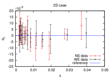
The simulation was run for several square lattices with size ranging from to . The estimators of and were acquired for mutually perpendicular directions, denoted by NS (top to bottom) and WE (left to right). The percolation threshold for the infinite lattice () was computed by fitting the data to the scaling properties described by Eqn. 5 as presented in Fig. 5. The results for the infinite lattice based on the intercept of the fitted linear function are the following:
| (11a) | ||||
| (11b) | ||||
It is worth noting that values converge to from both directions, as presented in Fig. 5. The obtained value of equal is clearly model-specific, as discussed in Section IV.2.

a)
b)
IV.2 Duality and exact analytic result
We consider a realization of the two dimensional graph defined by presented in Fig. 6a. We define the graph dual to the initial one according to the following procedure:
- •
dual lines are introduced, each line is placed between two existing lines;
- •
dual lines are divided into tubes (dual tubes) by the bonds of initial graph (vertical segments marked in Fig. 6b);
- •
at the positions on breaks between initial tubes the dual bonds connecting dual tubes are introduced (horizontal lines marked in Fig. 6b).
The two graphs, initial and dual, are shown in Fig 6a and c.

a) original graph b) construction c) dual graph
New tubes and bonds are generated in the same way as the original ones, with the two Poisson process parameters interchanged. Notice that the two graphs have no intersections. We either have a connection from top to bottom, using tubes and bonds of the original graph, or we can draw a line through the empty spaces and breaks between the tubes from left to right, that does not cross any bonds or tubes. In the latter case, there is a connection from left to right in the dual graph. Similarly, exactly one of the two alternatives occurs: either there is a connection from left to right by bonds and tubes of the original graph, or there is a connection from top to bottom in the dual graph— an unbroken path through empty spaces. A given realization starts to percolate when the dual graph stops percolating, so for a pair of dual graphs.
We know that the percolation threshold in the limit depends only on the ratio . Increasing results in more (shorter) tubes and thus makes percolation more difficult, while increasing makes for more connections between tubes, which facilitates it. Together with the duality described above, this indicates that , i.e. is the percolation threshold, thus explaining the numerical result (11a) and (11), and giving further support to our method. We emphasize that a rigorous proof that the critical value of equals requires a more careful argument. The first result of this type (for the square lattice) was proven in [28]. Simpler arguments developed later can be found in [1]. They can be adapted to cover the present case as well.
IV.3 Critical exponents
Based on the scaling law (Eqn. 4a and 4b) we obtain the correlation length exponent : . The exact value is known to be .
We determined two characteristics of the clusters: the first one, presented in Fig. 7 a), based on size of clusters and the second one, presented in Fig. 7 b), based on volume of clusters.
The Fisher exponent , is determined based on cluster size distribution presented in Fig. 7 a) as . The exact value is [2]. The agreement of the results with the known values of critical exponents supports the validity of the algorithm.
Moreover, we show that the slopes of lines fitted in Figs. 7 a) and b) are the same, thus the Fisher exponent determined based on cluster size distribution and the exponent which based on cluster volume distribution are also the same. This observation confirms the duality relation of percolation models on a given and dual graphs, discussed in Section IV.2.

a) Normalized number of clusters of size .

b) Normalized number of clusters of volume .
V Results in three dimensions
The simulation was run for cubic lattices with size ranging from to . The estimators of and were acquired for perpendicular directions, denoted by NS, WE and TB (top to bottom). As in (IV) we use scaling properties described by the Eqn. 4b to compute the percolation threshold for infinite lattice. The results are as follows:
| (12a) | ||||
| (12b) | ||||
| (12c) | ||||
The results obtained by fitting independently three linear functions, as presented in 8 a), can be improved using the following constraints:
- •
the lines fitted to the results perpendicular to tubes (NS and WE) have the same slope and intercept ;
- •
the line fitted to the results parallel to tubes (TB) have the same intercept .
Thus the improved estimated value of the percolation threshold is:
| (13a) | ||||
It is worth noting that, exactly as in the two-dimensional case, which we discussed in Section (IV.2), the values converge to from both directions. This is clearly visible in Fig. 8.

a)

b)
VI Discussion
VI.1 Computational cost
The computational cost of determining an approximate value of the critical point depends on the size of the lattice and on the desired accuracy of calculation which can be expressed in terms of standard deviation . Analysis of this computational complexity allows us to know what accuracy can be achieved in a given time. The obtained value of is approximated by the Monte Carlo estimator , which takes into account all runs of the algorithm:
| (14) |
where denotes the number of repetitions of the Rising Water algorithm. Thus , the final accuracy of , depends on the number of runs of the algorithm and on the variance as follows:
| (15) |
From the Eqn. 4b we know that depends on the size of the domain . The computational cost is proportional to the number of times the Rising Water algorithm is repeated and to the cost of a single run (of the order of , where is the dimensionality of the problem). Thus the computational cost to obtain the result with the accuracy is
| (16) |
The exponent depends on the dimension of the problem. For the two-dimensional case it is , while in three dimensions it equals approximately 0.72. The logarithmic factor in the expression for the computational cost (Eqn. 16) is due to sorting of random numbers in step 2c in Section 1. One method to avoid this is to use so-called bucket sort, which is a linear-time sorting algorithm using information about data distribution [27]. Due to statistical behavior of the random values we can create a set of disjoint intervals that cover all possible values of and have approximately the same expected number of random values in each interval. Let us denote this expected number of random variables in one interval (“bucket”) by . For every generated random () we can compute in constant time to which bucket it should be assigned. When all numbers are generated and classified, in each bucket we have a set of . numbers, and we need to sort it. The computational cost of generating random variables and sorting buckets of size is and it is linear in because it is always possible to generate enough intervals to keep M constant. After that, the cost of running the algorithm times is
and cost of running the algorithm to get desired accuracy is
Here is the Ackerman function and can be considered constant. Despite better asymptotic behavior of the bucket sort, it does not give a better performance except for very big lattices.
VII Conclusions
In summary, three goals have been achieved in this work:
- •
We have defined a family of discrete-continuous percolation models motivated by the physics of activated carbon. These models deal with tubes of random length connected by random bonds; as such they should describe well situations in which complicated micro-structures observed in activated carbon have approximately linear textures: graphene ribbons (model of Jenkins-Kawamura) and nanotubes [19]. In cases the structures are neither 1D nor quasi-1D (fullerenes (Harris model [15, 16]), stacked graphite [17], or graphene [14], carbon onions [18]), the concrete models considered here provide only a “caricature” of the real situation. Still we expect that even in these cases they capture some qualitative aspects of the underlying physics.
- •
We have extended the standard algorithm of Newman and Ziff [10] to handle inhomogeneous lattices. This extension is non-trivial, and we have analyzed in detail its convergence properties.
- •
We applied the extended algorithm to the family of models in question, calculating critical parameters and cluster density distributions in two and three dimensions.
Possibilities for further studies include: i) applications of the present models to experimental data, suggesting geometry formed by parallel random tubes/ribbons connected randomly by bonds; ii) development of concrete models with geometry formed by parallel random flakes/patches connected randomly by bonds; iii) application of the method to such models, calculation of their properties, and direct comparison with experiments.
It is worth mentioning that the problem of quantum aspects of the carbon activation process is also to a great extent open. This suggests to study quantum versions of the family of the discrete-continuous models discussed in this paper. The interplay of discrete and continuous aspects may lead to quantitatively novel effects. It is worth noting that such quantum disordered models can in principle be simulated, quantum simulated, by a system of ultracold atoms (see, for instance, [29]): an array of random length 1D Bose condensed gases with controlled random connections between them.
Acknowledgements.
This work has been partially supported by the Iuventus Plus programme founded by the Polish Ministry of Science and Higher Education (IP2014 024373). M.L. acknowledges Spanish MINECO Project FOQUS (FIS2013-46768), ERC AdG OSYRIS, EU IP SIQS, EU STREP EQuaM, and EU FETPROACT QUIC. J.W. has been partially funded by NSF grant DMS 131271.References
- [1] G. R. Grimmett, Percolation (Grundlehren der mathematischen Wissenschaften) (Springer: Berlin, Germany, 2010).
- [2] A. Aharony and D. Stauffer, Introduction to percolation theory (Taylor & Francis, United Kingdom, 2003).
- [3] R. Meester and R. Roy, Continuum percolation, Cambridge Tracts in Mathematics, Vol. 119 (Cambridge University Press, Cambridge, 1996).
- [4] Z. Wu, L. A. Braunstein, S. Havlin, and H. E. Stanley, Phys. Rev. Lett. 96, 148702 (2006).
- [5] D. Li, B. Fu, Y. Wang, G. Lu, Y. Berezin, H. E. Stanley, and S. Havlin, Proceedings of the National Academy of Sciences 112, 669 (2015), http://www.pnas.org/content/112/3/669.full.pdf .
- [6] M. Franceschetti, L. Booth, M. Cook, R. Meester, and J. Bruck, Journal of Statistical Physics 118, 721 (2005).
- [7] L. Booth, J. Bruck, M. Franceschetti, and R. Meester, The Annals of Applied Probability 13, pp. 722 (2003).
- [8] S. Furmaniak, A. P. Terzyk, P. A. Gauden, P. Kowalczyk, and P. J. Harris, Journal of Physics: Condensed Matter 26, 485006 (2014).
- [9] S. Furmaniak, A. P. Terzyk, P. A. Gauden, and P. Kowalczyk, Microporous and Mesoporous Materials 154, 51 (2012).
- [10] M. E. Newman and R. M. Ziff, Physical Review E 64, 016706 (2001).
- [11] B. Feng and S. K. Bhatia, Energy and Fuels 14, 297 (2000).
- [12] K. Kwiatkowski, K. Bajer, A. Celińska, M. Dudyński, J. Korotko, and M. Sosnowska, Fuel 132, 125 (2014).
- [13] H. Marsh, Activated carbon compendium: a collection of papers from the journal carbon 1996-2000 (Gulf Professional Publishing, 2001).
- [14] M. Pawlyta, Materials Science and Engineering 63, 58 (2013).
- [15] P. J. Harris, Chemistry and physics of carbon 28 (2003).
- [16] H. Marsh and F. R. Reinoso, Activated carbon (Elsevier, 2006).
- [17] G. Jenkins and K. Kawamura, Nature 231, 175 (1971).
- [18] Y. Chen, C. Liu, F. Li, and H.-M. Cheng, Journal of Porous Materials 13, 141 (2006).
- [19] P. J. Harris, Journal of Materials Science 48, 565 (2013).
- [20] X. Wang, G. Sun, and P. Chen, Frontiers in Energy Research 2, 33 (2014).
- [21] L. Berlyand and J. Wehr, Communications in Mathematical Physics 185, 73 (1997).
- [22] L. Berlyand and J. Wehr, Journal of Physics A: Mathematical and General 28, 7127 (1995).
- [23] J. Hoshen and R. Kopelman, Physical Review B 14, 3438 (1976).
- [24] Z. Alexandrowicz, Physics Letters A 80, 284 (1980).
- [25] P. Leath, Physical Review B 14, 5046 (1976).
- [26] M. E. J. Newman and R. M. Ziff, Phys. Rev. Lett. 85, 4104 (2000).
- [27] T. H. Cormen, Introduction to algorithms (MIT press, 2009).
- [28] H. Kesten, Communications in Mathematical Physics 74, 41 (1980).
- [29] M. Lewenstein, A. Sanpera, and V. Ahufinger, Ultracold atoms in optical lattices: Simulating quantum many-body systems (Oxford University Press, Oxford, 2012).