\ttitle

References

[1] I. Bierenbaum, S. Buchta, P. Draggiotis, I. Malamos, and G. Rodrigo, “Tree-Loop Duality Relation beyond simple poles”, JHEP 1303 (2013) 025, arXiv:1211.5048.
[2] S. Buchta, G. Chachamis, P. Draggiotis, I. Malamos, and G. Rodrigo, “On the singular behaviour of scattering amplitudes in quantum field theory”, JHEP 1411 (2014) 014, arXiv:1405.7850.
[3] S. Buchta, G. Chachamis, and G. Rodrigo in preparation.
[4] I. Bierenbaum, P. Draggiotis, S. Buchta, G. Chachamis, I. Malamos, et al., “News on the Loop-tree Duality”, Acta Phys.Polon. B44 (2013) 2207–2213.
[5] S. Buchta, G. Chachamis, I. Malamos, I. Bierenbaum, P. Draggiotis, et al., “The loop-tree duality at work”, PoS LL2014 (2014) 066, arXiv:1407.5865.
[6] S. Buchta, G. Chachamis, I. Malamos, P. Draggiotis, and G. Rodrigo, “Towards a Numerical Implementation of the Loop-Tree Duality Method”, Nucl.Part.Phys.Proc. 258-259 (2015) 33–36.
[7] F. Englert and R. Brout, “Broken Symmetry and the Mass of Gauge Vector Mesons”, Phys.Rev.Lett. 13 (1964) 321–323.
[8] P. W. Higgs, “Broken symmetries, massless particles and gauge fields”, Phys.Lett. 12 (1964) 132–133.
[9] G. Guralnik, C. Hagen, and T. Kibble, “Global Conservation Laws and Massless Particles”, Phys.Rev.Lett. 13 (1964) 585–587.
[10] A. H. Peter, “Dark Matter: A Brief Review”, arXiv:1201.3942.
[11] P. Fisher, B. Kayser, and K. S. McFarland, “Neutrino mass and oscillation”, Ann.Rev.Nucl.Part.Sci. 49 (1999) 481–528, arXiv:hep-ph/9906244.
[12] M. E. Peskin and D. V. Schroeder, “An Introduction to quantum field theory”, Westview Press, 1995.
[13] Particle Data Group Collaboration, J. Beringer et al., “Review of Particle Physics (RPP)”, Phys.Rev. D86 (2012) 010001.
[14] H. Fritzsch, M. Gell-Mann, and H. Leutwyler, “Advantages of the Color Octet Gluon Picture”, Phys.Lett. B47 (1973) 365–368.
[15] C.-N. Yang and R. L. Mills, “Conservation of Isotopic Spin and Isotopic Gauge Invariance”, Phys.Rev. 96 (1954) 191–195.
[16] K. G. Wilson, “Confinement of Quarks”, Phys.Rev. D10 (1974) 2445–2459.
[17] D. J. Gross and F. Wilczek, “Ultraviolet Behavior of Nonabelian Gauge Theories”, Phys.Rev.Lett. 30 (1973) 1343–1346.
[18] H. D. Politzer, “Reliable Perturbative Results for Strong Interactions?”, Phys.Rev.Lett. 30 (1973) 1346–1349.
[19] A. Salam and J. C. Ward, “Electromagnetic and weak interactions”, Phys.Lett. 13 (1964) 168–171.
[20] S. Weinberg, “A Model of Leptons”, Phys.Rev.Lett. 19 (1967) 1264–1266.
[21] A. Salam, “Weak and Electromagnetic Interactions”, Conf.Proc. C680519 (1968) 367–377.
[22] S. Glashow, “Partial Symmetries of Weak Interactions”, Nucl.Phys. 22 (1961) 579–588.
[23] J. S. Schwinger, “Quantum electrodynamics. I A covariant formulation”, Phys.Rev. 74 (1948) 1439.
[24] R. Feynman, “Relativistic cutoff for quantum electrodynamics”, Phys.Rev. 74 (1948) 1430–1438.
[25] R. Feynman, “Space - time approach to quantum electrodynamics”, Phys.Rev. 76 (1949) 769–789.
[26] ATLAS Collaboration, G. Aad et al., “Observation of a new particle in the search for the Standard Model Higgs boson with the ATLAS detector at the LHC”, Phys.Lett. B716 (2012) 1–29, arXiv:1207.7214.
[27] CMS Collaboration, S. Chatrchyan et al., “Observation of a new boson at a mass of 125 GeV with the CMS experiment at the LHC”, Phys.Lett. B716 (2012) 30–61, arXiv:1207.7235.
[28] Z. Bern, L. J. Dixon, D. C. Dunbar, and D. A. Kosower, “Fusing gauge theory tree amplitudes into loop amplitudes”, Nucl.Phys. B435 (1995) 59–101, arXiv:hep-ph/9409265.
[29] Z. Bern, L. J. Dixon, and D. A. Kosower, “On-Shell Methods in Perturbative QCD”, Annals Phys. 322 (2007) 1587–1634, arXiv:0704.2798.
[30] C. Anastasiou, R. Britto, B. Feng, Z. Kunszt, and P. Mastrolia, “Unitarity cuts and Reduction to master integrals in d dimensions for one-loop amplitudes”, JHEP 0703 (2007) 111, arXiv:hep-ph/0612277.
[31] G. Ossola, C. G. Papadopoulos, and R. Pittau, “Reducing full one-loop amplitudes to scalar integrals at the integrand level”, Nucl.Phys. B763 (2007)a 147–169, arXiv:hep-ph/0609007.
[32] G. Ossola, C. G. Papadopoulos, and R. Pittau, “Numerical evaluation of six-photon amplitudes”, JHEP 0707 (2007)b 085, arXiv:0704.1271.
[33] V. A. Smirnov, “Analytical result for dimensionally regularized massless on shell double box”, Phys.Lett. B460 (1999) 397–404, arXiv:hep-ph/9905323.
[34] J. Tausk, “Nonplanar massless two loop Feynman diagrams with four on-shell legs”, Phys.Lett. B469 (1999) 225–234, arXiv:hep-ph/9909506.
[35] T. Binoth and G. Heinrich, “An automatized algorithm to compute infrared divergent multiloop integrals”, Nucl.Phys. B585 (2000) 741–759, arXiv:hep-ph/0004013.
[36] T. Binoth and G. Heinrich, “Numerical evaluation of multiloop integrals by sector decomposition”, Nucl.Phys. B680 (2004) 375–388, arXiv:hep-ph/0305234.
[37] J. Carter and G. Heinrich, “SecDec: A general program for sector decomposition”, Comput.Phys.Commun. 182 (2011) 1566–1581, arXiv:1011.5493.
[38] S. Borowka, G. Heinrich, S. Jones, M. Kerner, J. Schlenk, et al., “SecDec-3.0: numerical evaluation of multi-scale integrals beyond one loop”, arXiv:1502.06595.
[39] C. Berger, Z. Bern, L. J. Dixon, F. Febres Cordero, D. Forde, et al., “Precise Predictions for $W$ + 3 Jet Production at Hadron Colliders”, Phys.Rev.Lett. 102 (2009) 222001, arXiv:0902.2760.
[40] K. Melnikov and G. Zanderighi, “W+3 jet production at the LHC as a signal or background”, Phys.Rev. D81 (2010) 074025, arXiv:0910.3671.
[41] G. Bevilacqua, M. Czakon, C. Papadopoulos, R. Pittau, and M. Worek, “Assault on the NLO Wishlist: pp — $>$ t anti-t b anti-b”, JHEP 0909 (2009) 109, arXiv:0907.4723.
[42] A. Bredenstein, A. Denner, S. Dittmaier, and S. Pozzorini, “NLO QCD Corrections to Top Anti-Top Bottom Anti-Bottom Production at the LHC: 2. full hadronic results”, JHEP 1003 (2010) 021, arXiv:1001.4006.
[43] S. Catani and M. Seymour, “A General algorithm for calculating jet cross-sections in NLO QCD”, Nucl.Phys. B485 (1997) 291–419, arXiv:hep-ph/9605323.
[44] S. Catani and M. Seymour, “The Dipole formalism for the calculation of QCD jet cross-sections at next-to-leading order”, Phys.Lett. B378 (1996) 287–301, arXiv:hep-ph/9602277.
[45] S. Frixione, Z. Kunszt, and A. Signer, “Three jet cross-sections to next-to-leading order”, Nucl.Phys. B467 (1996) 399–442, arXiv:hep-ph/9512328.
[46] A. Gehrmann-De Ridder, T. Gehrmann, and E. N. Glover, “Antenna subtraction at NNLO”, JHEP 0509 (2005) 056, arXiv:hep-ph/0505111.
[47] S. Catani and M. Grazzini, “An NNLO subtraction formalism in hadron collisions and its application to Higgs boson production at the LHC”, Phys.Rev.Lett. 98 (2007) 222002, arXiv:hep-ph/0703012.
[48] S. Catani, T. Gleisberg, F. Krauss, G. Rodrigo, and J.-C. Winter, “From loops to trees by-passing Feynman’s theorem”, JHEP 0809 (2008) 065, arXiv:0804.3170.
[49] I. Bierenbaum, S. Catani, P. Draggiotis, and G. Rodrigo, “A Tree-Loop Duality Relation at Two Loops and Beyond”, JHEP 1010 (2010) 073, arXiv:1007.0194.
[50] UA1 Collaboration, G. Arnison et al., “Experimental Observation of Isolated Large Transverse Energy Electrons with Associated Missing Energy at s**(1/2) = 540-GeV”, Phys.Lett. B122 (1983)a 103–116.
[51] UA1 Collaboration, G. Arnison et al., “Experimental Observation of Lepton Pairs of Invariant Mass Around 95-GeV/c**2 at the CERN SPS Collider”, Phys.Lett. B126 (1983)b 398–410.
[52] TASSO Collaboration, R. Brandelik et al., “Evidence for Planar Events in e+ e- Annihilation at High-Energies”, Phys.Lett. B86 (1979) 243.
[53] D. Barber, U. Becker, H. Benda, A. Boehm, J. Branson, et al., “Discovery of Three Jet Events and a Test of Quantum Chromodynamics at PETRA Energies”, Phys.Rev.Lett. 43 (1979) 830.
[54] PLUTO Collaboration, C. Berger et al., “Evidence for Gluon Bremsstrahlung in e+ e- Annihilations at High-Energies”, Phys.Lett. B86 (1979) 418.
[55] JADE Collaboration, W. Bartel et al., “Observation of Planar Three Jet Events in e+ e- Annihilation and Evidence for Gluon Bremsstrahlung”, Phys.Lett. B91 (1980) 142.
[56] SLAC-SP-017 Collaboration, J. Augustin et al., “Discovery of a Narrow Resonance in e+ e- Annihilation”, Phys.Rev.Lett. 33 (1974) 1406–1408.
[57] E598 Collaboration, J. Aubert et al., “Experimental Observation of a Heavy Particle J”, Phys.Rev.Lett. 33 (1974) 1404–1406.
[58] CDF Collaboration, F. Abe et al., “Observation of top quark production in $\bar{p}p$ collisions”, Phys.Rev.Lett. 74 (1995) 2626–2631, arXiv:hep-ex/9503002.
[59] D0 Collaboration, S. Abachi et al., “Search for high mass top quark production in $p\bar{p}$ collisions at $\sqrt{s}=1.8$ TeV”, Phys.Rev.Lett. 74 (1995) 2422–2426, arXiv:hep-ex/9411001.
[60] D. Hanneke, S. Fogwell, and G. Gabrielse, “New Measurement of the Electron Magnetic Moment and the Fine Structure Constant”, Phys.Rev.Lett. 100 (2008) 120801, arXiv:0801.1134.
[61] T. Kinoshita and D. Yennie, “High precision tests of quantum electrodynamics: An Overview”, Adv.Ser.Direct.High Energy Phys. 7 (1990) 1–14.
[62] ALEPH, DELPHI, L3, OPAL, SLD, LEP Electroweak Working Group, SLD Electroweak Group, SLD Heavy Flavour Group Collaboration, S. Schael et al., “Precision electroweak measurements on the $Z$ resonance”, Phys.Rept. 427 (2006) 257–454, arXiv:hep-ex/0509008.
[63] L. Faddeev and V. Popov, “Feynman Diagrams for the Yang-Mills Field”, Phys.Lett. B25 (1967) 29–30.
[64] S. Weinzierl, “Automated calculations for multi-leg processes”, PoS ACAT (2007) 005, arXiv:0707.3342.
[65] Z. Bern and D. A. Kosower, “Color decomposition of one loop amplitudes in gauge theories”, Nucl.Phys. B362 (1991) 389–448.
[66] F. A. Berends and W. Giele, “Recursive Calculations for Processes with n Gluons”, Nucl.Phys. B306 (1988) 759.
[67] F. Cachazo, P. Svrcek, and E. Witten, “MHV vertices and tree amplitudes in gauge theory”, JHEP 0409 (2004) 006, arXiv:hep-th/0403047.
[68] R. Britto, F. Cachazo, and B. Feng, “New recursion relations for tree amplitudes of gluons”, Nucl.Phys. B715 (2005) 499–522, arXiv:hep-th/0412308.
[69] S. Weinzierl, “Introduction to theoretical elementary particle physics”, Lecture held at the Johannes Gutenberg-University of Mainz, 2012.
[70] S. Weinzierl, “Introduction to Monte Carlo methods”, arXiv:hep-ph/0006269.
[71] T. Hahn, “CUBA: A Library for multidimensional numerical integration”, Comput.Phys.Commun. 168 (2005) 78–95, arXiv:hep-ph/0404043.
[72] T. Gleisberg, “Automating methods to improve precision in Monte-Carlo event generation for particle colliders”, Ph.D. Thesis, 2007 Dresden.
[73] G. Rodrigo, S. Catani, T. Gleisberg, F. Krauss, and J.-C. Winter, “From multileg loops to trees (by-passing Feynman’s Tree Theorem)”, Nucl.Phys.Proc.Suppl. 183 (2008) 262–267, arXiv:0807.0531.
[74] R. Feynman, “Quantum theory of gravitation”, Acta Phys.Polon. 24 (1963) 697–722.
[75] R. Feynman, “Closed Loop and Tree Diagrams. (Talk) in Magic Without Magic, ed. J. R. Klauder, (Freeman, San Francisco), p. 355, in Selected papers of Richard Feynman, ed. L. M. Brown (World Scientific, Singapore, 2000) p. 867.”, 1972.
[76] I. Bierenbaum, “Towards a Loop-Tree Duality at Two Loops and Beyond”, Nucl.Phys.Proc.Suppl. 205-206 (2010) 164–169, arXiv:1007.0213.
[77] K. Chetyrkin and F. Tkachov, “Integration by Parts: The Algorithm to Calculate beta Functions in 4 Loops”, Nucl.Phys. B192 (1981) 159–204.
[78] V. Smirnov, “Feynman integral calculus”, Springer, 2006.
[79] A. Smirnov, “Algorithm FIRE – Feynman Integral REduction”, JHEP 0810 (2008) 107, arXiv:0807.3243.
[80] A. von Manteuffel and C. Studerus, “Reduze 2 - Distributed Feynman Integral Reduction”, arXiv:1201.4330.
[81] C. W. Bauer, A. Frink, and R. Kreckel, “Introduction to the GiNaC framework for symbolic computation within the C++ programming language”, arXiv:cs/0004015.
[82] J. Gluza, K. Kajda, and D. A. Kosower, “Towards a Basis for Planar Two-Loop Integrals”, Phys.Rev. D83 (2011) 045012, arXiv:1009.0472.
[83] W. Gong, Z. Nagy, and D. E. Soper, “Direct numerical integration of one-loop Feynman diagrams for N-photon amplitudes”, Phys.Rev. D79 (2009) 033005, arXiv:0812.3686.
[84] Z. Nagy and D. E. Soper, “Numerical integration of one-loop Feynman diagrams for N-photon amplitudes”, Phys.Rev. D74 (2006) 093006, arXiv:hep-ph/0610028.
[85] M. Kramer and D. E. Soper, “Next-to-leading order numerical calculations in Coulomb gauge”, Phys.Rev. D66 (2002) 054017, arXiv:hep-ph/0204113.
[86] D. E. Soper, “Choosing integration points for QCD calculations by numerical integration”, Phys.Rev. D64 (2001) 034018, arXiv:hep-ph/0103262.
[87] D. E. Soper, “Techniques for QCD calculations by numerical integration”, Phys.Rev. D62 (2000) 014009, arXiv:hep-ph/9910292.
[88] D. E. Soper, “QCD calculations by numerical integration”, Phys.Rev.Lett. 81 (1998) 2638–2641, arXiv:hep-ph/9804454.
[89] S. Becker and S. Weinzierl, “Direct contour deformation with arbitrary masses in the loop”, Phys.Rev. D86 (2012) 074009, arXiv:1208.4088.
[90] S. Becker and S. Weinzierl, “Direct numerical integration for multi-loop integrals”, Eur.Phys.J. C73 (2013), no. 2, 2321, arXiv:1211.0509.
[91] S. Mandelstam, “Unitarity Condition Below Physical Thresholds in the Normal and Anomalous Cases”, Phys.Rev.Lett. 4 (1960) 84–87.
[92] H. Rechenberg and E. Sudarshan, “Analyticity in quantum field theory. 1. The triangle graph revisited”, Nuovo Cim. A12 (1972) 541–568.
[93] S. Catani, D. de Florian, and G. Rodrigo, “The Triple collinear limit of one loop QCD amplitudes”, Phys.Lett. B586 (2004) 323–331, arXiv:hep-ph/0312067.
[94] G. F. Sborlini, D. de Florian, and G. Rodrigo, “Double collinear splitting amplitudes at next-to-leading order”, JHEP 1401 (2014) 018, arXiv:1310.6841.
[95] J. Berntsen, T. O. Espelid, and A. Genz, “An Adaptive Algorithm for the Approximate Calculation of Multiple Integrals”, ACM Trans. Math. Softw. 17 (1991)a 437–451.
[96] J. Berntsen, T. O. Espelid, and A. Genz, “ An Adaptive Multidimensional Integration Routine for a Vector of Integrals”, ACM Trans. Math. Softw. 17 (1991)b 452–456.
[97] I. Wolfram Research, “Mathematica”, Wolfram Research, Inc., version 8.0 ed., 2010.
[98] T. Hahn, “Generating and calculating one loop Feynman diagrams with FeynArts, FormCalc, and LoopTools”, arXiv:hep-ph/9905354.

\univname

Doctoral Thesis

\ttitle

Author:

\authornames

Supervisor:
\supname

3026 Programa Oficial de Doctorado en Física

\deptname\groupname

June 2015

Abstract

La Dualidad Loop-Árbol (LTD) representa un nuevo método perturbativo en Teoria Cuántica de Campos que establece una relación entre amplitudes de dispersión virtuales y de árbol. Se logra hacer esto por aplicación directa del Teorema de los Residuos a la integratión de la componente de energía. El resultado es la suma de todos los cortes simples posibles del diagrama de Feynman considerado integrada sobre un espacio fásico modificado. Estas integrales de corte simple, denominadas Contribuciones Duales, de hecho son objetos de tipo árbol y por lo tanto dan lugar a la oportunidad de combinar las contribuciones virtuales y de árbol con el motivo de tratarlas simultáneamente en un generador de eventos de Monte Carlo. A pesar de ser introducido inicialmente para integrales escalares de un loop, la practicabilidad de la LTD fue extendida tremendamente. En esta tesis demonstramos como aplicar la LTD a diagramas con polos de multiplicidad elevada utilizando relaciones de Integración Por Partes (IBP). Además, examinamos la cancelación de singularidades entre Contribuciones Duales tanto como entre correcciones reales y virtuales. Por primera vez una implementación numérica de la LTD fue realizada en forma de un programa de ordenador que calcula diagramas de dispersión. Presentamos detalles sobre la deformación de contorno empleada y los resultados de integrales escalares hasta el nivel de pentágono y de integrales tensoriales hasta el nivel de hexágono.

I certify that I have read this dissertation and that, in
my opinion it is fully adequate in scope and quality as a
dissertation for the degree Doctor of Philosophy.

Germán Rodrigo

(Supervisor)

Author:

Supervisor:

Co-Supervisors:

Sebastian Buchta
Germán Rodrigo
Stefano Catani
Grigorios Chachamis

\Declaration

I, \authornames, declare that this thesis titled, ’\ttitle’ and the work presented in it are my own. I confirm that:

$\blacksquare$

This work is original and was done wholly or mainly while in candidature for a research degree at this University.
$\blacksquare$

Where any part of this thesis has previously been submitted for a degree or any other qualification at this University or any other institution, this has been clearly stated.
$\blacksquare$

Where I have consulted the published work of others, this is always clearly attributed.
$\blacksquare$

Where I have quoted from the work of others, the source is always given. With the exception of such quotations, this thesis is entirely my own work.
$\blacksquare$

I have acknowledged all main sources of help.
$\blacksquare$

Where the thesis is based on work done by myself jointly with others, I have made clear exactly what was done by others and what I have contributed myself.

Signed:

Date:

This thesis is based on the author’s work conducted at the IFIC (Instituto de Física Corpuscular, Universitat de València, Consejo Superior de Investigaciones Científicas). Parts of it have already been published in articles and proceedings earlier.

Articles

Proceedings

\addtotoc

Abstract

Acknowledgements.

First and foremost, I would like to express my deep gratitude to Dr. Germán Rodrigo, my research supervisor, for his patient guidance and astute advice throughout this project. In particular, I am grateful for his continuous support, encouragement and his way of thinking outside the box. Especially I would like to thank my co-supervisor Dr. Grigorios Chachamis for investing a lot of time into discussions and detailed explanations as well as answering countless questions inside and outside of physics. I further thank my colleagues Dr. Petros Draggiotis and Dr. Ioannis Malamos for frequently helping me on with the difficulties I faced at work. I would also like to thank Daniel Götz, who explained me how to use the Cuba library in C++. Special thanks go to Dr. Sophia Borowka and Dr. Gudrun Heinrich for all the help they provided me while I was using SecDec to produce reference values to compare to. I do appreciate the financial support that I received and which allowed me to freely carry out my studies. In particular, this has been

•

the position as an Early Stage Researcher within the LHCPhenoNet during the first year, and
•

the JAE Predoc 2011 fellowship for the rest of the Ph.D.

Also in this context, I highly value the unique possibilities that being a part of the LHCPhenoNet offered me in terms of conferences, summer schools and general exposure to the scientific community.

Finally, I am grateful for the unconditional support of my family during the entirety of my Ph.D.

Chapter 0 Introduction

The Large Hadron Collider (LHC), the largest and most complex machine ever built by mankind, gives particle physicists a powerful tool at hand to verify existing models and probe the fundamental laws at very high energies. The aim of the LHC is: First, to investigate whether the Standard Model (SM) is still valid at the collider’s energies. Second, to shed light on the electroweak symmetry breaking mechanism and to find or exclude a particle that fits the SM description of the Higgs boson [7, 8, 9]. Third, to search for Beyond Standard Model (BSM) physics like supersymmetry or extra-dimensions or particles that could be Dark Matter candidates. In the first run of the LHC, a Higgs-like particle has been found with a mass of 125 GeV. Apart from that, several other discoveries have been made including the first creation of a quark-gluon plasma or the rare $\text{B}_{S}$ -decay. In the second run, in which the center-of-mass energies will be increased even further, signals of BSM physics are hoped to be detected and the properties of the Higgs further explored.
Despite the existence of observations which the SM cannot accommodate at the moment, e.g. the existence Dark Matter [10] or neutrino oscillations [11], it is still the only established theory of particle physics to date that describes experimental data, a great theoretical achievement of its own. Leaving out gravity, for which there is no quantum theory available yet, it successfully describes (almost) all relevant particle physical observables.
The SM is a relativistic quantum field theory with an $SU(3)\times SU(2)\times U(1)$ gauge symmetry. It describes three of the four fundamental forces of nature at microscopic distances, namely electromagnetism, strong and weak force.¹¹ 1 For a full review of the Standard Model, see for example [12, 13].
The $SU(3)$ symmetry accounts for the strong force and the corresponding quantum field theory is called QCD (Quantum Chromodynamics, [14]). It describes the interactions between quarks and gluons. Quarks are, besides leptons, the fundamental matter constituents and come in six different flavors. Gluons are massless spin 1 particles (bosons) carrying an $SU(3)$ colour charge and act as the mediators of the strong force. Because the gauge group is non-Abelian [15], QCD features two remarkable properties: Confinement [16] and Asymptotic Freedom [17, 18].
Confinement accounts for the fact that physical objects are always colour-neutral at low energies, in particular no individual free quarks or gluons are observed. Nonetheless, an analytical proof of this property is still missing.
Asymptotic Freedom is a property of the theory. It means that due to the running of the strong coupling $\alpha_{s}$ , the strong force becomes small at high energies (equivalentely, small distances), a fact that permits the employment of perturbative techniques.
The weak force describes processes such as the decay of nuclei and the interaction of neutrinos with matter. In the modern context, it is better understood within the framework of the electroweak sector. By electroweak sector, we mean the unification of weak and electromagnetic forces [19, 20, 21, 22] by Weinberg, Salam and Glashow, a major success which allowed to understand both forces in the common framework of the Electroweak Symmetry Breaking mechanism. Very similar to the strong force, its gauge group is the non-Abelian $SU(2)$ . Contrary to QCD, the $W^{\pm}$ - and $Z^{0}$ -gauge bosons of the weak interaction are not only massive, but with masses of 80 GeV and 91 GeV respectively, they are quite heavy. Hence it is a short distance interaction and appears to be ‘weak’.
Finally, $U(1)$ is the gauge group of Quantum Electrodynamics (QED) [23] which is the quantum field theory describing the electromagnetic force. Its gauge boson, the photon, is massless and due to the Abelian nature of $U(1)$ , photons do not interact with each other and the force is of unlimited range.
What we today know as the Standard Model of particle physics is QCD together with the electroweak sector. It has undergone countless checks and investigations over many different aspects and it has been exceptionally successful in making correct and accurate predictions for a wide range of physical observables.
However, the SM is believed to be a mere low-energy approximation to a still to be constructed unified field theory which would describe all four forces at all energy regimes. The SM-Lagrangian encodes all previosly known symmetry principles, for example conservation laws. Although its mathematical formulation is very simple, we cannot analytically solve the equations of motion. Only in certain parts of phase-space we can perform reliable theoretical calculations which are all based on perturbation theory. The underlying idea is that when the coupling of the interaction term is small, one can do a series expansion in which every term can be represented in a pictorial form. This is done by the so-called Feynman diagrams [24, 25]. Due to its clarity and predictive power, the diagrammatical approach is the most popular for theoretical calculations. The first term of the expansion usually gives an estimate of the order of magnitude whereas in order to obtain the first proper estimate, one has formally to go to next-to-leading order (NLO) precision. More and more processes processes demand next-to-next-to-leading order (NNLO) precision to match the precision of the experimental data.
The discovery of the Higgs-like boson in 2012 has been a huge success [26, 27]. At the moment of writing this thesis, the LHC is warming up for its second phase with a center-of-mass energy of up to 13 TeV. In this second phase, as previously mentioned, it will be of great importance to measure as many properties of the discovered particle as possible and to continue the hunt for physics beyond the Standard Model. So far, the absence of signals hinting to BSM physics is a little disappointing as it does not define a clear direction for the theorists to follow.
The high quality of LHC data raises the need for high-precision theoretical predictions. The processes at the LHC are rather challenging to calculate because they typically involve many particles and because QCD plays the dominant role at the LHC. Furthermore, higher orders of the perturbation expansion have to be calculated in order to match the experimental precision. This has led to considerable progress in the analytical and numerical techniques for the calculation of Standard Model cross-sections. Apart from the usual diagrammatic approach, there are other methods, some of the most popular ones being Unitarity Methods [28, 29, 30], the OPP-Method [31, 32], Mellin-Barnes Representations [33, 34] and Sector Decomposition [35, 36, 37, 38]. Thanks to these techniques, 2 $\to$ 4 processes at NLO are the standard nowadays, and even higher multiplicities are becoming more accessible [39, 40, 41, 42]. They have achieved an incredible feat: The computation of Feynman graphs up to NNLO-level and in some cases even beyond. Still, many important issues remain. When calculating cross-sections one needs to consider tree- and loop-contributions separately. Thus, a lot of effort has to be put into cancelling infrared singularities between real and virtual corrections [43, 44, 45, 46, 47]. Additional difficulties arise from threshold singularities that lead to numerical instabilities.
Recently, a new method called the Loop–Tree Duality (LTD) [48] has been developed, which is designed to attack these problems. The basic concept at one-loop is to directly apply the Cauchy Residue Theorem to the Feynman integrals. The outcome is a sum of tree level objects in which each represents all possible single cuts of the considered diagram. This form is called the ‘dual integral’, which closely resembles the real corrections. The idea is to then combine the dual integral with the tree-level contributions in order to treat them simultaneously in a common Monte Carlo event generator. While initially the technique was limited to one-loop graphs, it has been greatly expanded since then. In [49] it has been shown how to extend it to diagrams with an arbitrary number of loops and in [1] how to deal with graphs which involve propagators that are raised to higher powers (higher order poles).

1 Outline

The remainder of this thesis is organised as follows: In Chapter 1, we establish the fundamentals of this work. In Chapter 2 we introduce the Loop–Tree Duality method alongside some illustrative examples. In Chapter 3, we formalize the notation and extend the Loop–Tree Duality to double and higher order loop graphs. in Chapter 4 we show how to deal with poles of higher multiplicities. In Chapter 5 we report on the cancellation of singularities among dual contributions as well as between real and virtual corrections for massless internal lines. In Chapter 6, we present details on the numerical implementation of the Loop–Tree Duality for scalar one-loop integrals. This is the first time that the LTD has been applied to explicitly calculate Feynman diagrams and constitutes the main result of this thesis. In Chapter 7, we demonstrate that the computer program used in Chapter 6 is also able to deal with tensor integrals. We conclude the thesis with Chapter 8 in which we give a summary and our future plans.

Chapter 1 Standard Model Phenomenology

The Standard Model is a theory of particle physics that has been refined continuously over the past, so that it is nowadays able to describe almost all particle reaction processes that we observe in the laboratory (particle colliders) as well as in space. Its tremendous success is threefold:

•

The SM has the ability to explain a wide variety of experimental results.
•

The SM repeatedly predicted the existence of particles before their experimental discovery. This has been the case for the $W^{\pm}$ and $Z^{0}$ bosons [50, 51], the gluon [52, 53, 54, 55] and the charm [56, 57] and top quarks [58, 59] and very recently the Higgs boson [27, 26]. For each of these particles, experiments later confirmed the predicted properties with good precision.
•

The SM has passed a huge number of precision tests with flying colours, the most famous one being the anomalous magnetic dipole moment of the electron [60]: The agreement between theory and measurement is up to the 13th digit, which is a unique achievement not only in particle physics, but in all science. Other examples of precisely predicted quantities are the Neutron Compton Wavelength [61] or the mass of the $Z^{0}$ boson [62].

All of these accomplishments have strengthend the confidence in the SM as the proper theory for the description of the behaviour of elementary particles excluding gravity.
We dedicate the next section to an instructive review of the basic principles of the SM.

1 The Standard Model of Particle Physics

The Standard Model of particle physics is a quantum field theory which nowadays allows us to correctly describe almost all physical processes with high precision on a fundamental level. It is based on the gauge group

\displaystyle SU(3)\times SU(2)\times U(1)

(1)

where $SU(3)$ is the gauge group of the strong interaction, $SU(2)$ the gauge group of the weak isospin, and $U(1)$ the gauge group of the hypercharge which is not identical with the gauge group of QED. To avoid confusion, the notations $U(1)_{Y}$ and $U(1)_{EM}$ with subscripts hinting to either the hypercharge ( $Y$ ) or QED ( $EM$ ) will be used.
Despite the interacting constituents being fields, the SM’s perturbative description is carried out almost entirely in the particle picture. We imagine the force between two matter particles to be mediated via exchange particles. All interactions have in common that the matter fields are spin $\frac{1}{2}$ fermions and the exchange particles spin $1$ bosons, with the exception of the Higgs boson which has spin $0$ .

1 QCD

The QCD, Quantum ChromoDynamics, is a non-Abelian gauge theory with the action

\displaystyle S=\int d^{4}x\left\{\bar{\psi}(i\not{D}-m)\psi-\frac{1}{4}\text{tr}F_{\mu\nu}F^{\mu\nu}\right\}~,

(2)

and the symmetry group $SU(3)$ . The fermion fields $\psi$ transform under its fundamental representation. They are, apart from the gluons, the dynamical degrees of freedom of the theory. There are six flavors of quarks, each with a different mass. $D$ is the so-called covariant derivative, defined as

\displaystyle D_{\mu}=\partial_{\mu}-ig_{s}A_{\mu}~,

(3)

with $A_{\mu}=A_{\mu}^{a}T^{a}$ being the gluon field, which lives in the adjoint representation of the gauge group. The group $SU(N)$ has $N^{2}-1$ generators, hence $SU(3)$ has eight of them. They span the Lie algebra $\mathfrak{su}(3)$ and are normalised by $\text{tr}(T^{a}T^{b})=\delta^{ab}$ and $[T^{a},T^{b}]=if^{abc}T^{c}$ . $F_{\mu\nu}$ is the field strength tensor. It is an algebra-valued two-form defined by

\displaystyle F_{\mu\nu}=\frac{1}{ig_{s}}[D_{\mu},D_{\nu}]=\partial_{\mu}A_{\nu}-\partial_{\nu}A_{\mu}+ig_{s}[A_{\mu},A_{\nu}].

(4)

The first two terms are a four-dimensional rotation known from QED; the third term is typical for non-Abelian symmetry groups and the origin of the gluon self-interaction.
Considering QCD in the absence of quarks, the only thing left is the gluon self-interaction. This branch is called pure Yang-Mills theory. As we mentined in the Introduction, QCD has two special properties, Confinement and Asymptotic Freedom. They mainly have to do with the running coupling $\alpha_{s}(Q)$ of QCD. By running coupling we mean that the coupling is dependent on the energy at which the process happens [12]:

\displaystyle\alpha_{s}(Q)=\frac{2\pi}{(11-2n_{f}/3)\ln(Q/\Lambda_{QCD})}~.

(5)

Confinement takes place at low energies at which the coupling is strong. Physical states are always color singlets: As a consequence of the non-Abelian gauge symmetry, the energy cost grows proportionally to the distance, if one tries to separate the particles of a color singlet. At some point it is energetically favorable for a new quark-antiquark pair to appear. Hence, neither free quarks nor free gluons are observed in nature.
Asymptotic freedom describes the phenomenon that the coupling of the theory becomes weaker as the energy increases. At very high energies, quarks and gluons are almost able to move as if they were free particles. In this energy regime, perturbation theory is applicable. However, one has to quantise the action first, a good method to do so is the one by Faddeev and Popov [63]. An unwanted side effect of the method is the introduction of ghost fields into the theory. They are called ghosts because of their incorrect spin-statistic relation and therefore are unphysical. To get rid of them, one can choose the axial gauge, in which ghosts and gluons decouple and the gauge of the action is fixed. From the gauge fixed action one can extract the propagators and vertices which allow to calculate the contributions to the perturbation series via the Feynman diagram approach. These diagarams are pictorial representations of the terms of the perturbation series. To calculate an amplitude of arbitrary order in $\alpha_{s}$ , one draws all the Feynman diagrams that contribute to the process, contracts them with the outer polarisation vectors and spinors and finally sums them up.

	$\frac{i}{\not{p}-m}\delta_{ij}$
	$-\frac{i}{p^{2}}g^{\mu\nu}\delta^{ab}$

Figure 1: QCD propagators in Feynman gauge, without ghosts.

	$ig\gamma^{\mu}T^{a}$
	$gf^{abc}[g^{\mu\nu}(p-k)^{\rho}$ $\hskip 23.49976pt\,\,\,\,+g^{\nu\rho}(q-p)^{\mu}$ $\hskip 23.49976pt\,\,\,\,+g^{\rho\mu}(k-q)^{\nu}]$
	$-ig^{2}[f^{abe}f^{cde}(g^{\mu\rho}g^{\nu\sigma}-g^{\mu\sigma}g^{\nu\rho})$ $\,\,\,\hskip 11.74988pt+f^{ade}f^{bce}(g^{\mu\nu}g^{\rho\sigma}-g^{\mu\rho}g^{\nu\sigma})$ $\hskip 11.74988pt\,\,\,+f^{ace}f^{bde}(g^{\mu\nu}g^{\rho\sigma}-g^{\mu\sigma}g^{\nu\rho})]$

Figure 2: QCD vertices in Feynman gauge, without ghosts. All momenta outgoing.

A downside of this approach is that it consumes a lot of computational power. For example, the number of Feynman diagrams that contribute to the $n$ -gluon amplitude grows faster than $n$ ![64]. Techniques like color-ordered amplitudes [65] and (tree-level) recurrence relations [66, 67, 68] have been developed to deal with that problem.

2 Electroweak Interaction

Until 1967, QED and weak interaction were two separate theories. In that year, Salam, Weinberg and Glashow succeeded in understanding both interactions as special cases of one unified theory called Electroweak theory [19, 20, 21, 22]. The reason why both interactions appear to be so different is the spontaneously broken symmetry of the Electroweak theory.
The corresponding action resembles the one of the QCD:

\displaystyle S=\int d^{4}x\left\{\bar{\psi}(i\not{D}-m)\psi-\frac{1}{4}\text{tr}W_{\mu\nu}W^{\mu\nu}-\frac{1}{4}\text{tr}B_{\mu\nu}B^{\mu\nu}\right\}+(D_{\mu}\phi)^{\dagger}D^{\mu}\phi-m^{2}\phi^{\dagger}\phi+\frac{\lambda}{4}(\phi^{\dagger}\phi)^{2}~.

The matter fields $\psi$ of the electroweak interaction are the six leptons, but quarks do carry a weak charge as well. They can be organised into three generations. Electron, muon and tau participate in both the weak and the electromagnetic interactions. The corresponding neutrinos interact exclusively weakly. Within the SM, they are supposed to be massless, though recent experiments show that they actually have a small nonzero mass. This allows to solve the solar neutrino problem using the concept of neutrino oscillations [11]. The operator $D$ is defined as:

\displaystyle D_{\mu}=\partial_{\mu}-igW_{\mu}^{a}\sigma^{a}-\frac{ig^{\prime}}{2}B_{\mu}Y~.

(6)

The underlying symmetry group of the electroweak interaction is the $SU(2)\times U(1)_{Y}$ . In Eq. (6), the $\sigma^{a}$ are the generators of the $SU(2)$ and the hypercharge $Y$ is the generator of the $U(1)_{Y}$ . Because of the direct product of the two groups, they carry different coupling constants $g$ and $g^{\prime}$ .
The fields $W$ and $B$ are the gauge fields of the theory. $W$ is a field similar gluons of QCD with respect to their non-Abelian character. The corresponding field strength tensor is obtained by replacing $A$ with $W$ in equation (4). The field $B$ transforms under the Abelian symmetry group $U(1)_{Y}$ . Thus its field strength tensor does not have a commutator.
According to the way $B$ and $W$ appear in the Lagrangian, they are massless. However, experiments show that the $W$ and $Z$ bosons indeed have a mass. To get rid of this flaw of the theory, one introduces an additional field $\phi$ , the so-called Higgs-field, that couples to the gauge bosons by the term $(D_{\mu}\phi)D^{\mu}\phi$ . The a priori unphysical and massless fields $B$ and $W$ now obtain their masses via the Higgs-mechanism. By transforming the unphysical fields $B$ and $W$ in physical ones, the $SU(2)\times U(1)_{Y}$ -symmetry is broken down to a $U(1)_{EM}$ -symmetry. Simultaneously the Lagrangian picks up the correct mass terms for the $W$ and $Z$ bosons as well as the photon. The other terms of the Langrangian represent the potential of the Higgs field. This is illustrated in greater detail in the next subsection.
Despite the similarities between QCD and electroweak interaction, the latter one does not display the phenomenon “Confinement”. The reason for this is that the exchange bosons of the electroweak interaction are very heavy, namely 80 GeV for the $W^{\pm}$ and 91 GeV for the $Z^{0}$ , which does not allow for bound states. “Asymptotic Freedom”, however, is observed for the weak interaction just as in QCD.

3 Higgs Boson and Electroweak Symmetry Breaking

In the Standard Model, the gauge group $SU(2)\times U(1)_{Y}$ is spontaneously broken. The left-over symmetry is $U(1)_{EM}$ . One assumes the existence of an additional complex scalar field which transforms under SU(2) and has hypercharge $Y=1$ . In the space of weak isospin, it can be represented by a two-component vector with complex entries [69].

\displaystyle\phi(x)=\begin{pmatrix}\phi^{+}(x)\\ \frac{1}{\sqrt{2}}(v+H(x)+i\chi(x))\end{pmatrix}~,

(7)

$\phi^{+}(x)$ is a complex field, i.e. it is composed of two components. The three components $\phi^{+}(x)$ and $\chi(x)$ are absorbed into the longitudinal modes of $W^{\pm}_{\mu}$ and $Z_{\mu}$ . $H(x)$ is the actual physical Higgs-field. The Lagrangian of the Higgs-sector then reads

\displaystyle\mathcal{L}_{\text{Higgs}}=(D_{\mu}\phi)^{\dagger}(D^{\mu}\phi)\underbrace{-m^{2}\phi^{\dagger}\phi+\frac{\lambda}{4}(\phi^{\dagger}\phi)^{2}}_{V(\phi)}+\mathcal{L}_{\text{Yukawa}}~,

(8)

For the theory to be bound from below, $\lambda$ has to be greater than zero, $\lambda>0$ , and furthermore $m^{2}<0$ for the symmetry to be spontaneously broken. The covariant derivative is given by Eq. (6). The Higgs-dublet has hypercharge $Y=1$ ; from the minimization of the potential $V(\phi)$ follows

\displaystyle|\phi_{\text{min}}|^{2}=\frac{2m^{2}}{\lambda}=\frac{v^{2}}{2}\Rightarrow v=2\sqrt{\frac{m^{2}}{\lambda}}~.

(9)

In the next step, the physical contributions to $(D_{\mu}\phi)^{\dagger}D^{\mu}\phi$ will be calculated.

	$\displaystyle(D_{\mu}\phi)^{\dagger}(D^{\mu}\phi)\|_{\text{phys}}$	$\displaystyle=\frac{1}{2}\partial_{\mu}H\partial^{\mu}H+\frac{1}{2}\left(\frac{gv}{2}\right)^{2}(W_{\mu}^{1}W^{1\mu}+W_{\mu}^{2}W^{2\mu})+$
		$\displaystyle+\frac{1}{8}(B_{\mu},W_{\mu}^{3})\begin{pmatrix}g^{\prime 2}&-gg^{\prime}\\ -gg^{\prime}&g^{2}\end{pmatrix}\begin{pmatrix}B^{\mu}\\ W^{3\mu}\end{pmatrix}$		(10)

$H$ is already a physical field, but $B$ and $W$ are not. They are transformed to physical fields by virtue of the transformations

\displaystyle W_{\mu}^{\pm}=\frac{1}{\sqrt{2}}(W_{\mu}^{1}\mp W_{\mu}^{2})

(11)

and

\displaystyle\begin{pmatrix}A_{\mu}\\ Z_{\mu}\end{pmatrix}=\begin{pmatrix}\cos\theta_{W}&\sin\theta_{W}\\ -\sin\theta_{W}&\cos\theta_{W}\end{pmatrix}\begin{pmatrix}B_{\mu}\\ W_{\mu}^{3}\end{pmatrix}~.

(12)

Here, $\sin\theta_{W}$ and $\cos\theta_{W}$ are given by

\displaystyle\cos\theta_{W}=\frac{g}{\sqrt{g^{2}+g^{\prime 2}}}\qquad\text{and}\qquad\sin\theta_{W}=\frac{g^{\prime}}{\sqrt{g^{2}+d^{\prime 2}}}~.

(13)

This way, one can rewrite the part of the Lagrangian of equation (10) as

	$\displaystyle(D_{\mu}\phi)^{\dagger}(D^{\mu}\phi)\|_{\text{phys}}$	$\displaystyle=\frac{1}{2}\partial_{\mu}H\partial^{\mu}H+\frac{1}{2}\left(\frac{gv}{2}\right)^{2}(W_{\mu}^{+}W^{+\mu}+W_{\mu}^{-}W^{-\mu})$
		$\displaystyle+\frac{1}{2}\left(\frac{v}{2}\sqrt{g^{2}+g^{\prime 2}}\right)^{2}(A_{\mu},Z_{\mu})\begin{pmatrix}0&0\\ 0&1\end{pmatrix}\begin{pmatrix}A^{\mu}\\ Z^{\mu}\end{pmatrix}~.$		(14)

Now, the masses of the $W$ - and $Z$ -bosons can be read off easily:

\displaystyle m_{W}=\frac{v}{2}g\qquad\text{and}\qquad m_{Z}=\frac{v}{2}\sqrt{g^{2}+g^{\prime 2}}~.

(15)

The couplings $g$ and $g^{\prime}$ are related to the elementary charge $e$ by

\displaystyle e=\frac{gg^{\prime}}{\sqrt{g^{2}+g^{\prime 2}}}\quad\text{or}\quad g=\frac{e}{\sin\theta_{W}}\quad\text{and}\quad g^{\prime}=\frac{e}{\cos\theta_{W}}\quad\text{respectively.}

(16)

Within this framework, it is possible to have massive gauge bosons which otherwise are forbidden by unbroken gauge symmetries.

2 Particle Phenomenology

Phenomenology is the branch of particle physics that deals with the calculation of physical observables that can then be compared to experimental measurements. In order to test a theory, solutions have to be compared to experimental data. For the SM, there are two established ways to calculate them: Lattice calculations and perturbation theory. Since lattice techniques lie beyond the scope of this thesis, we focus on the latter. As mentioned in Section 1, perturbation theory (in the coupling) is employed at high energies when the coupling of the theory becomes small. Usually, Feynman diagrams are used to calculate the individual contributions to the perturbation series. We distinguish betweeen two main types of diagrams: Tree and loop diagrams. The the leading order term is a tree-level contribution. Beyond leading order, a Feynman diagram gets dressed with more lines. These can connect two existing lines, thus leading to a loop or they connect to only one existing line resulting in an additional external leg. We use the terms next-to-leading order (NLO, one-loop) or next-to-next-to-leading order (NNLO, two-loops) to indicate the accuracy up to which a certain calculation has been performed. Today, the quality of data collected at colliders like the LHC has reached a level that makes the inclusion of terms beyond the leading order of perturbation theory necessary in order to provide theoretical estimates of similar precision. Apart from the cancellation of singularities between tree and loop corrections and phase-space integrations with many external legs, loop diagrams are the bottleneck when calculating scattering amplitudes. Hence, theorists are looking for ways to efficiently calculate NLO and NNLO corrections. The last decade in particular has seen a huge progress in the development of calculational techniques to tackle computations at NLO and also some progress at NNLO accuracy. In the LHC era, this is important, because of the availability of large amounts of data to which theoretical predictions can be compared to. Still, the task of obtaining theoretical estimates that can be compared with LHC-data is not easy. Tree and loop contributions have to be evaluated independently before bringing them together. The Loop–Tree Duality method, which will be introduced in Chapter 2 and which is at the heart of this thesis, reexpresses loop-level objects in terms of tree-level objects. Thus it allows to directly combine the two, in order to evaluate them simultaneously. This evaluation is carried out using numerical integration. In the latter chapters of the thesis, we present results of the of the first implementation of the Loop–Tree Duality method as a computer progam. This program calculates one-loop integrals using a numerical integrator (Cuhre or VEGAS). Since the numerical integrator is employed as a black box, we recapitulate the basics of numerical integration in Section 3.

3 Numerical Integration Techniques

1 Motivation for employing numerical techniques

In Chapters 6 and 7, we are going to calculate a certain type of three-dimensional integral.
Usually one is interested in knowing the value of an integral up to a certain accuracy and wants to obtain the result within an acceptable amount of time. Hence, a numerical integrator in the form of a computer program is the proper tool for this task.
Our long-term goal is to set up a fully automated program which is able to calculate (N)NLO cross-sections for arbitrary kinematics. In this thesis, we do the first step by addressing the virtual part.

2 Classical numerical integration

For the rest of this chapter, we closely follow the paper [70] by Weinzierl, which is a nice introduction to the subject and is recommended to readers with further interest in the matter.

Quadrature rules have been known for a long time. The numerical integrator “Cuhre”, part of the Cuba-library [71], uses quadrature rules to estimate the integral, therefore their idea shall be illustrated here. One distinguishes between formulae that evaluate the integrand at equally spaced abscissas (Newton-Cotes type) and formulae which evaluate the integrand at carefully selected, but non-equally spaced abscissas (Gaussian quadrature rules). The simplest example of a Newton-Cotes type rule is the so-called trapezoidal rule:

\int\limits_{x_{0}}^{x_{0}+\Delta x}dxf(x)=\frac{\Delta x}{2}[f(x_{0})+f(x_{0}+\Delta x)]-\frac{(\Delta x)^{3}}{12}f^{\prime\prime}(\xi)~,

(17)

where $x_{0}\leq\xi\leq x_{0}+\Delta x$ . To approximate an integral over a finite interval $[x_{0},x_{n}]$ with the help of this formula, one divides the interval into $n$ sub-intervals of length $\Delta x$ and applies the trapezoidal rule to each sub-interval. With the notation $x_{j}=x_{0}+j\cdot\Delta x$ , one arrives at the compound formula

\int\limits_{x_{0}}^{x_{n}}dxf(x)=\frac{x_{n}-x_{0}}{n}\sum\limits_{j=0}^{n}w_{j}f(x_{j})-\frac{1}{12}\frac{(x_{n}-x_{0})^{3}}{n^{2}}\tilde{f}^{\prime\prime}

(18)

with $w_{0}=w_{n}=1/2$ and $w_{j}=1$ for $1\leq j\leq n-1$ . Further

\tilde{f}^{\prime\prime}=\frac{1}{n}\sum\limits_{j=1}^{n}f^{\prime\prime}(\xi_{j}),

(19)

where $\xi_{j}$ is somewhere in the interval $[x_{j-1},x_{j}]$ . Since the position of the $\xi_{j}$ cannot be known without knowing the integral exactly, the last term in Eq. (18) is usually neglected and introduces an error in the numerical evaluation. This error is proportional to $1/n^{2}$ and one has to evaluate the function $f(x)$ roughly $n$ -times.
An improvement is given by Simpson’s rule, which evaluates the function at three points:

\int\limits_{x_{0}}^{x_{2}}dxf(x)=\frac{\Delta x}{3}[f(x_{0})+4f(x_{1})+f(x_{2})]-\frac{(\Delta x)^{5}}{90}f^{(4)}(\xi).

(20)

This yields the compound formula

\int\limits_{x_{0}}^{x_{2}}dxf(x)=\frac{x_{n}-x_{0}}{n}\sum\limits_{j=0}^{n}w_{j}f(x_{j})-\frac{1}{180}\frac{(x_{n}-x_{0})^{5}}{n^{4}}\tilde{f}^{(4)}

(21)

where $n$ is an even number, $w_{0}=w_{n}=1/3$ , and for $1\leq j\leq n$ we have $w_{j}=4/3$ if $j$ is odd and $w_{j}^{\prime}$ if $j=2/3$ is even. The error estimate scales now as $1/n^{4}$ .

As mentioned earlier, there are also rules involving non-equally spaced abscissas. A well known representative is the main formula of Gaussian quadrature.
If $w(x)$ is a weight function on $[a,b]$ , then there exist weights $w_{j}$ and abscissas $x_{j}$ for $1\leq j\leq n$ such that

\int\limits_{a}^{b}dx\,w(x)\,f(x)=\sum\limits_{j=1}^{n}w_{j}f(x_{j})+\frac{f^{(2n)}(\xi)}{(2n)!}\int\limits_{a}^{b}dx\,w(x)\,[\Pi(x)]^{2}

(22)

with

		$\displaystyle\Pi(x)=(x-x_{1})(x-x_{2})\dots(x-x_{n}),$
		$\displaystyle a\leq x_{1}<x_{2}<\dots<x_{n}\leq b,\quad a<\xi<b$		(23)

The abscissas are given by the zeros of the orthogonal polynomial of degree $n$ associated to the weight function $w(x)$ . In order to find them numerically, it is useful to know that they all lie in the interval $[a,b]$ . The weights are given by the (weighted) integral over the Lagrange polynomials:

\displaystyle w_{j}=\int\limits_{a}^{b}dx\,w(x)l_{j}^{n}(x)

(24)

where the fundamental Lagrange polynomials are given by

\displaystyle l_{i}^{n}(x)=\frac{(x-x_{0})\dots(x-x_{i-1})(x-x_{i+1})\dots(x-x_{n})}{(x_{i}-x_{0})\dots(x_{i}-x_{i-1})(x_{i}-x_{i+1})\dots(x_{i}-x_{n})}

(25)

3 Monte Carlo techniques

Monte Carlo integration is one of the two methods to perform the integrations in Chapters 6 and 7, although we also present only the results of CI. This is common for the evaluation of multi-dimensional integrals. Generally speaking one is looking for an algorithm that meets a certain set of properties. It should

•

give a numerical estimate of the integral together with an estimate of the error,
•

yield the result in a reasonable amount of time, e.g. at low computational cost,
•

be able to handle multidimensional integrals.

Monte Carlo integration delivers on all points of the list. In particular, as will be shown later, its error scales like $1/\sqrt{N}$ , independent of the number of dimensions. This makes Monte Carlo integration the preferred method for integrals in high dimensions.

Another integrator provided by the Cuba-library [71] is “VEGAS”. It is a Monte Carlo integrator paired with variance reducing techniques. These two concepts shall be shown in the following subsection.
Quadrature rules are inefficient for multidimensional integrals. Therefore one resorts to Monte Carlo integration. On the plus side, its error scales like $1/\sqrt{N}$ independent of the number of dimensions. But, on the other hand, a convergence by a rate of $1/\sqrt{N}$ is pretty slow. To improve efficiency, variance reducing techniques like importance sampling are employed.
Consider the integral of a function $f(u_{1},\dots,u_{d})$ , depending on $d$ variables $u_{1},\dots,u_{d}$ over the unit hypercube $[0,1]^{d}$ . Furthermore, $f$ is assumed to be square-integrable. From now on, the short-hand notation $x=(u_{1},\dots,u_{d})$ and for the function evaluated at that point $f(x)=f(u_{1},\dots,u_{d})$ will be used. The Monte Carlo estimate for the integral

\displaystyle I=\int dxf(x)=\int d^{d}uf(u_{1},\dots,u_{d})

(26)

is given by

\displaystyle E=\frac{1}{N}\sum\limits_{n=1}^{N}f(x_{n})~.

(27)

The law of large numbers ensures that the Monte Carlo estimate converges to the true value of the integral:

\displaystyle\lim\limits_{N\rightarrow\infty}\frac{1}{N}\sum\limits_{n=1}^{N}f(x_{n})=I~.

(28)

The corresponding error $S$ reads

\displaystyle S^{2}=\frac{1}{N}\sum\limits_{n=1}^{N}(f(x_{n}))^{2}-E^{2}~.

(29)

Stratified sampling

This technique consists of dividing the full integration space into subspaces, performing a Monte Carlo integration in each subspace, and adding up partial results in the end. Mathematically, this is based on the fundamental property of the Riemann integral

\displaystyle\int\limits_{0}^{1}dxf(x)=\int\limits_{0}^{a}dxf(x)+\int\limits_{a}^{1}dxf(x),\quad 0<a<1.

(30)

More generally, one splits the integration region $M=[0,1]^{d}$ into $k$ regions $m_{j}$ where $j=1,\dots,k$ . In each region one performs a Monte Carlo integration with $n_{j}$ points. For the integral $I$ , one obtains the estimate

\displaystyle E=\sum\limits_{j=1}^{k}\frac{\operatorname{vol}(M_{j})}{N_{j}}\sum\limits_{n=1}^{N_{j}}f(x_{jn})

(31)

and instead of $S^{2}$ one has now the expression

\displaystyle\sum\limits_{j=1}^{k}\frac{\operatorname{vol}(M_{j})}{N_{j}}\cdot\left.N\cdot S^{2}\right|_{M_{j}}

(32)

If the subspaces and the number of points in each subspace are chosen carefully, this can lead to a dramatic reduction in the error compared with crude Monte Carlo, but it should be noted, that it can also lead to a larger error if the choice is not appropriate. In general, the total variance is minimized when the number of points in each sub-volume is proportional to $\left.N\cdot S^{2}\right|_{M_{j}}$ .

Importance sampling

Mathematically, importance sampling corresponds to a change of integration variables:

\displaystyle\int\limits dx\,f(x)=\int\frac{f(x)}{p(x)}p(x)dx=\int\frac{f(x)}{p(x)}dP(x)

(33)

with

\displaystyle p(x)=\frac{\partial^{d}}{\partial x_{1}\dots\partial x_{d}}P(x)

(34)

If one restricts $p(x)$ to be a positive-valued function $p(x)\geq 0$ and to be normalized to unity

\int dx\,p(x)=1

(35)

one may interpret $p(x)$ as a probability density function. If one has a random number generator corresponding to the distribution $P(x)$ at his disposal, one may estimate the integral from a sample $x_{1},\dots,x_{N}$ of random numbers distributed according to $P(x)$ :

E=\frac{1}{N}\sum\limits_{n=1}^{N}\frac{f(x)}{p(x)}.

(36)

The statistical error $S$ of the Monte Carlo integration is given by

S^{2}\left(\frac{f}{p}\right)=\frac{1}{N}\sum\limits_{n=1}{N}\left(\frac{f(x_{n})}{p(x_{n})}\right)^{2}-E^{2}.

(37)

It becomes evident that the relevant quantity is now $f(x)/p(x)$ and it will be advantageous to choose $p(x)$ as close in shape to $f(x)$ as possible. In practice, one chooses $p(x)$ such that it approximates $|f(x)|$ reasonably well in shape and such that one can generate random numbers distributed according to $P(x)$ .
One disadvantage of importance sampling is the fact, that it is dangerous to choose functions $p(x)$ , which become zero, or which approach zero quickly. If $p$ goes to zero where $f$ is not zero, $S^{2}(f/p)$ may be infinite and the usual technique of estimating the variance from the sample points may not detect this fact if the region where $p=0$ is small.

The VEGAS-algorithm

The techniques described before require some advanced knowledge of the behaviour of the function to be integrated. In many cases this information is not available and one prefers adaptive techniques, e.g. an algorithm which learns about the functions as it proceeds. In the following, the VEGAS-algorithm will be presented. It combines the basic ideas of importance sampling and stratified sampling into an iterative algorithm, which automatically concentrates evaluations of the integrand in those regions where the integrand is largest in magnitude. VEGAS starts by subdividing the integration space into a rectangular grid and performs an integration in each subspace. These results are then used to adjust the grid for the next iteration according to where the integral receives dominant contributions. In this way VEGAS uses importance sampling and tries to approximate the optimal probability density function

p_{\text{optimal}}(x)=\frac{|f(x)|}{\int dx|f(x)|}

(38)

by a step function. Due to storage requirements one has to use a separable probability density function in $d$ dimensions:

p(u_{1},\dots,u_{d})=p_{1}(u_{1})\cdot p_{2}(u_{2})\cdot\dots\cdot p_{d}(u_{d}).

(39)

Eventually after a few iterations the optimal grid is found. In order to avoid rapid destabilizing changes in the grid, the adjustment of the grid includes usually a damping term. After this initial exploratory phase, the grid may be frozen and in a second evaluation phase the integral may be evaluated with high precision according to the optimized grid. The separation in an exploratory phase and an evaluation phase allows one to use less integrand evaluations in the first phase and to ignore the numerical estimates from this phase (which will in general have a larger variance). Each iteration yields an estimate $E_{j}$ together with an estimate for the variance $S_{j}^{2}$ :

E_{j}=\frac{1}{N_{j}}\sum\limits_{n=1}^{N_{j}}\frac{f(x_{n})}{p(x_{n})},\qquad S_{j}^{2}=\frac{1}{N_{j}}\sum\limits_{n=1}^{N_{j}}\left(\frac{f(x_{n})}{p(x_{n})}\right)^{2}-E^{2}_{j}.

(40)

Here $N_{j}$ denotes the number of integrand evaluations on iteration $j$ . The results of each iteration on the evaluation phase are combined into a cumulative estimate, weighted by the number of calls $N_{j}$ and their variances:

E=\left(\sum\limits_{j=1}^{m}\frac{N_{j}}{S_{j}^{2}}\right)^{-1}\left(\sum\limits_{j=1}^{m}\frac{N_{j}E_{j}}{S_{j}^{2}}\right).

(41)

If the error estimates $S_{j}^{2}$ become unreliable (for example if the function is not square integrable), it is more appropriate to weight the partial results by the number $N_{j}$ of integrand evaluations alone. In addition VEGAS returns the $\chi^{2}$ per degree of freedom:

\chi^{2}/\operatorname{dof}=\frac{1}{m-1}\sum\limits_{j=1}^{m}\frac{(E_{j}-E)^{2}}{S_{j}^{2}}.

(42)

This allows a check whether the various estimates are consistent. One expects a $\chi^{2}/\operatorname{dof}$ not much greater than one.

Chapter 2 Loop–Tree Duality at One–Loop

This chapter serves to introduce the Loop-Tree Duality method (LTD) [72, 73] which we will be using subsequently throughout this thesis. It is a technique to numerically calculate multi-leg one-loop cross-sections in perturbative field theories. In fact, it is applicable in any quantum field theory in Minkowsky space with an arbitrary number of space-time dimensions. At its core, it establishes a relation between loop-level and tree-level amplitudes similar to the Feynman Tree Theorem (FTT) [74, 75]. Both methods allow to write basisc loop Feynman diagrams in terms of tree-level phase-space integrals which are obtained by cutting the original loop-integral. This is achieved by directly applying the Residue Theorem¹¹ 1 Within the context of loop integrals, the use of the residue theorem has been considered many times in textbooks and in the literature. . to the loop integrand. However, there are also some inportant differences between them: While the LTD produces only single cuts, the FTT also involves higher order cuts (double, triple, and so forth).

In this chapter, we closely follow Refs. [48, 49] ²² 2 Ref. [48] is a good introduction to the Duality relation. It gives further insight into its nature and its comparison to the FTT. We refer the interested reader to that paper. For the purpose of this thesis we will follow it (and [49]) only as far as necessary to understand the later chapters. to illustrate and derive the Loop–Tree Duality.

1 Notation

The FTT and the LTD can be illustrated with no loss of generality by considering their application to the basic ingredient of any one-loop Feynman diagrams, namely a generic one-loop scalar integral $L^{(1)}$ with $N$ ( $N\geq 2$ ) external legs. In the following and throughout this thesis, we assume the considered diagrams to be free from UV and IR divergencies.

Refer to caption — Figure 1: Momentum configuration of the one-loop $N$ -point scalar integral.

The momenta of the external legs are denoted by $p_{1}^{\mu},p_{2}^{\mu},\dots,p_{N}^{\mu}$ and are clockwise ordered (Fig. 1). All are taken as outgoing. To simplify the notation and the presentation, we also limit ourselves in the beginning to considering massless internal lines only. Thus, the one-loop integral $L^{(1)}$ can in general be expressed as:

L^{(1)}(p_{1},p_{2},\dots,p_{N})=-i\,\int\frac{d^{d}\ell}{(2\pi)^{d}}\;\prod_{i=1}^{N}\,\frac{1}{q_{i}^{2}+i0}\;\;,

(1)

where $\ell^{\mu}$ is the loop momentum (which flows anti-clockwise). The momenta of the internal lines are denoted by $q_{i}^{\mu}$ ; they are given by

q_{i}=\ell+\sum_{k=1}^{i}p_{k}\;\;,

(2)

and momentum conservation results in the constraint

\sum_{i=1}^{N}p_{i}=0\;\;.

(3)

The value of the label $i$ of the external momenta is defined modulo $N$ , i.e. $p_{N+i}\equiv p_{i}$ .

The number of space-time dimensions is denoted by $d$ (the convention for the Lorentz-indices adopted here is $\mu=0,1,\dots,d-1$ ) with metric tensor $g^{\mu\nu}={\rm diag}(+1,-1,\dots,-1)$ . The space-time coordinates of any momentum $k_{\mu}$ are denoted as $k_{\mu}=(k_{0},{\bf k})$ , where $k_{0}$ is the energy (time component) of $k_{\mu}$ . It is also convenient to introduce light-cone coordinates $k_{\mu}=(k_{+},\bf{k}_{\perp},k_{-})$ , where $k_{\pm}=(k_{0}\pm k_{d-1})/{\sqrt{2}}$ . Throughout the chapter we consider loop integrals and phase-space integrals. If the integrals are ultraviolet or infrared divergent, we always assume that they are regularized by using analytic continuation in the number of space-time dimensions (dimensional regularization). Therefore, $d$ is not fixed and does not necessarily have integer value.

We introduce the following shorthand notation:

-i\,\int\frac{d^{d}\ell}{(2\pi)^{d}}\;\;\bullet\equiv\int_{\ell}\;\;\bullet\;\;.

(4)

When we factorize off in a loop integral the integration over the momentum coordinate $\ell_{0}$ or $\ell_{+}$ , we write

-i\,\int_{-\infty}^{+\infty}d\ell_{0}\;\int\frac{d^{d-1}{\boldsymbol{\ell}}}{(2\pi)^{d}}\;\;\bullet\equiv\int d\ell_{0}\;\int_{\vec{\boldsymbol{\ell}}}\;\;\bullet\;\;,

(5)

and

-i\,\int_{-\infty}^{+\infty}d\ell_{+}\;\int_{-\infty}^{+\infty}d\ell_{-}\int\frac{d^{d-2}{\boldsymbol{\ell}_{\perp}}}{(2\pi)^{d}}\;\;\bullet\equiv\int d\ell_{+}\;\int_{(\ell_{-},\boldsymbol{\ell}_{\perp})}\;\;\bullet\;\;,

(6)

respectively. The customary phase-space integral of a physical particle with momentum $\ell$ (i.e. an on-shell particle with positive-definite energy: $\ell^{2}=0$ , $\ell_{0}\geq 0$ ) reads

\int\frac{d^{d}\ell}{(2\pi)^{d-1}}\;\theta(\ell_{0})\;\delta(\ell^{2})\;\;\bullet\equiv\int_{\ell}\widetilde{\delta}(\ell)\;\;\bullet\;\;,

(7)

where we have defined

{\widetilde{\delta}}(\ell)\equiv 2\pi\,i\,\theta(\ell_{0})\;\delta(\ell^{2})=2\pi\,i\;\delta_{+}(\ell^{2})\;\;.

(8)

Using this shorthand notation, the one-loop integral $L^{(1)}$ in Eq. (1) can be cast into

L^{(1)}(p_{1},p_{2},\dots,p_{N})=\int_{\ell}\;\;\prod_{i=1}^{N}\,G_{F}(q_{i})\;\;,

(9)

where $G_{F}(q)$ denotes the customary Feynman propagator,

G_{F}(q)\equiv\frac{1}{q^{2}+i0}\;\;.

(10)

We also introduce the advanced propagator $G_{A}(q)$ ,

G_{A}(q)\equiv\frac{1}{q^{2}-i0\,q_{0}}\;\;.

(11)

We recall that the Feynman and advanced propagators only differ in the position of the particle poles in the complex plane (Fig. 2). Using $q^{2}=q_{0}^{2}-{\bf q}^{2}=2q_{+}q_{-}-{\bf q}_{\perp}^{2}$ , we therefore have

\left[G_{F}(q)\right]^{-1}=0\quad\Longrightarrow\quad q_{0}=\pm{\sqrt{{\bf q}^{2}-i0}}\;\;,{\rm or}\;\;q_{\pm}=\frac{{\bf q}_{\perp}^{2}-i0}{2q_{\mp}}\;\;,

(12)

and

\left[G_{A}(q)\right]^{-1}=0\quad\Longrightarrow\quad q_{0}\simeq\pm{\sqrt{{\bf q}^{2}}}+i0\;\;,{\rm or}\;\;q_{\pm}\simeq\frac{{\bf q}_{\perp}^{2}}{2q_{\mp}}+i0\;\;.

(13)

Thus, in the complex plane of the variable $q_{0}$ (or, equivalently³³ 3 To be precise, each propagator leads to two poles in the plane $q_{0}$ and to only one pole in the plane $q_{+}$ (or $q_{-}$ )., $q_{\pm}$ ), the pole with positive (negative) energy of the Feynman propagator is slightly displaced below (above) the real axis, while both poles (independently of the sign of the energy) of the advanced propagator are slightly displaced above the real axis.

Figure 2: Location of the particle poles of the Feynman (left) and advanced (right) propagators,

G_{F}(q)

and

G_{A}(q)

, in the complex plane of the variable

q_{0}

q_{\pm}

2 The Feynman Tree Theorem

In this section we briefly recall the FTT [74, 75]. To this end, we first introduce the advanced one-loop integral $L_{A}^{(1)}$ , which is obtained from $L^{(1)}$ in Eq. (9) by replacing the Feynman propagators $G_{F}(q_{i})$ with the corresponding advanced propagators $G_{A}(q_{i})$ :

L_{A}^{(1)}(p_{1},p_{2},\dots,p_{N})=\int_{\ell}\;\;\prod_{i=1}^{N}\,G_{A}(q_{i})\;\;.

(14)

Then, we note that

L_{A}^{(1)}(p_{1},p_{2},\dots,p_{N})=0\;\;.

(15)

The proof of Eq. (15) can be carried out in an elementary way by using the Cauchy Residue Theorem and choosing a suitable integration path $C_{L}$ . We have

	$\displaystyle L_{A}^{(1)}(p_{1},p_{2},\dots,p_{N})=\int_{\vec{\boldsymbol{\ell}}}\;\;\;\int d\ell_{0}\;\;\;\prod_{i=1}^{N}\,G_{A}(q_{i})$				(16)
		$\displaystyle=$	$\displaystyle\int_{\vec{\boldsymbol{\ell}}}\;\int_{C_{L}}d\ell_{0}\;\;\;\prod_{i=1}^{N}\,G_{A}(q_{i})=-\,2\pi i\;\int_{\vec{\boldsymbol{\ell}}}\;\;\sum\;{\rm Res}_{\{{\rm Im}\;\ell_{0}<0\}}\;\left[\;\prod_{i=1}^{N}\,G_{A}(q_{i})\right]=0\;\;.$		(16)

The loop integral is evaluated by integrating first over the energy component $\ell_{0}$ . Since the integrand is convergent when $\ell_{0}\to\infty$ , the $\ell_{0}$ integration can be performed along the contour $C_{L}$ , which is closed at $\infty$ in the lower half-plane of the complex variable $\ell_{0}$ (Fig. 3–left). The only singularities of the integrand with respect to the variable $\ell_{0}$ are the poles of the advanced propagators $G_{A}(q_{i})$ , which are located in the upper half-plane. The integral along $C_{L}$ is then equal to the sum of the residues at the poles in the lower half-plane and therefore it vanishes.

The advanced and Feynman propagators are related by

G_{A}(q)=G_{F}(q)+{\widetilde{\delta}}(q)\;\;,

(17)

which can straightforwardly be obtained by using the elementary identity

\frac{1}{x\pm i0}={\rm PV}\left(\frac{1}{x}\right)\mp i\pi\,\delta(x)\;\;,

(18)

where ${\rm PV}$ denotes the principal-value prescription. Inserting Eq. (17) into the right-hand side of Eq. (14) and collecting the contributions with an equal number of factors $G_{F}(q_{i})$ and ${\widetilde{\delta}}(q_{j})$ , we obtain a relation between $L_{A}^{(1)}$ and the one-loop integral $L^{(1)}$ :

	$\displaystyle L_{A}^{(1)}(p_{1},p_{2},\dots,p_{N})=\int_{\ell}\;\;\prod_{i=1}^{N}\,\left[G_{F}(q_{i})+{\widetilde{\delta}}(q_{i})\right]$		(19)
	$\displaystyle=L^{(1)}(p_{1},p_{2},\dots,p_{N})+L_{\rm{1-cut}}^{(1)}(p_{1},p_{2},\dots,p_{N})+\dots+L_{\rm{N-cut}}^{(1)}(p_{1},p_{2},\dots,p_{N})\;\;.$

Here, the single-cut contribution is given by

L_{\rm{1-cut}}^{(1)}(p_{1},p_{2},\dots,p_{N})=\int_{\ell}\;\;\sum_{i=1}^{N}\;{\widetilde{\delta}}(q_{i})\;\prod_{\stackrel{{\scriptstyle j=1}}{{j\neq i}}}^{N}\,G_{F}(q_{j})\;\;.

(20)

In general, the $m$ -cut terms $L_{\rm{m-cut}}^{(1)}$ $(m\leq N)$ are the contributions with precisely $m$ delta functions ${\widetilde{\delta}}(q_{i})$ :

L_{\rm{m-cut}}^{(1)}(p_{1},p_{2},\dots,p_{N})=\int_{\ell}\;\;\left\{{\widetilde{\delta}}(q_{1})\dots{\widetilde{\delta}}(q_{m})\;G_{F}(q_{m+1})\dots G_{F}(q_{N})+{\rm uneq.\;perms.}\right\}\;\;,

(21)

where the sum in the curly brackets includes all the permutations of $q_{1},\dots,q_{N}$ that give unequal terms in the integrand.

Recalling that $L_{A}^{(1)}$ vanishes, cf. Eq. (15), Eq. (19) results in:

L^{(1)}(p_{1},p_{2},\dots,p_{N})=-\left[\;L_{\rm{1-cut}}^{(1)}(p_{1},p_{2},\dots,p_{N})+\dots+L_{\rm{N-cut}}^{(1)}(p_{1},p_{2},\dots,p_{N})\;\right]\;\;.

(22)

This equation is the FTT in the specific case of the one-loop integral $L^{(1)}$ . The FTT relates the one-loop integral $L^{(1)}$ to the multiple-cut⁴⁴ 4 If the number of space-time dimensions is $d$ , the right-hand side of Eq. (22) receives contributions only from the terms with $m\leq d$ ; the terms with larger values of $m$ vanish, since the corresponding number of delta functions in the integrand is larger than the number of integration variables. integrals $L_{\rm{m-cut}}^{(1)}$ . Each delta function ${\widetilde{\delta}}(q_{i})$ in $L_{\rm{m-cut}}^{(1)}$ replaces the corresponding Feynman propagator in $L^{(1)}$ by cutting the internal line with momentum $q_{i}$ . This is synonymous to setting the respective particle on shell. An $m$ -particle cut decomposes the one-loop diagram in $m$ tree diagrams: in this sense, the FTT allows us to calculate loop-level diagrams from tree-level diagrams.

In view of the discussion in the following sections, it is useful to consider the single-cut contribution $L_{\rm{1-cut}}^{(1)}$ on the right-hand side of Eq. (22). In the case of single-cut contributions, the FTT replaces the one-loop integral with the customary one-particle phase-space integral, see Eqs. (7) and (20). Using the invariance of the loop-integration measure under translations of the loop momentum $\ell$ , we can perform the momentum shift $\ell\to\ell-\sum_{k=1}^{i}p_{k}$ in the term proportional to ${\widetilde{\delta}}(q_{i})$ on the right-hand side of Eq. (20). Thus, cf. Eq. (2), we have $q_{i}\to\ell$ and $q_{j}\to\ell+(p_{i+1}+p_{i+2}+\dots+p_{i+j})$ , with $i\neq j$ . We can repeat the same shift for each of the terms $(i=1,2,\dots,N)$ in the sum on the right-hand side of Eq. (20), and we can rewrite $L_{\rm{1-cut}}^{(1)}$ as a sum of $N$ basic phase-space integrals (Fig. 4):

	$\displaystyle L_{\rm{1-cut}}^{(N)}(p_{1},p_{2},\dots,p_{N})$	$\displaystyle=$	$\displaystyle I_{\rm{1-cut}}^{(N-1)}(p_{1},p_{1}+p_{2},\dots,p_{1}+p_{2}+\dots+p_{N-1})+\,{\rm cyclic\;perms.}$		(23)
		$\displaystyle=$	$\displaystyle\sum_{i=1}^{N}\;I_{\rm{1-cut}}^{(N-1)}(p_{i},p_{i}+p_{i+1},\dots,p_{i}+p_{i+1}+\dots+p_{i+N-2})\;\;.$		(23)

We denote the basic one-particle phase-space integrals with $n$ Feynman propagators by $I_{\rm{1-cut}}^{(n)}$ . They are defined as follows:

I_{\rm{1-cut}}^{(n)}(k_{1},k_{2},\dots,k_{n})=\int_{\ell}{\widetilde{\delta}}(\ell)\;\prod_{j=1}^{n}G_{F}(\ell+k_{j})=\int_{\ell}{\widetilde{\delta}}(\ell)\;\prod_{j=1}^{n}\frac{1}{2\ell\cdot k_{j}+k_{j}^{2}+i0}\;\;.

(24)

The extension of the FTT from the one-loop integrals $L^{(1)}$ to one-loop scattering amplitudes ${\cal A}^{({\rm 1-loop})}$ (or Green’s functions) in perturbative field theories is straightforward, provided the corresponding field theory is unitary and local. The generalization of Eq. (22) to arbitrary scattering amplitudes is [74, 75]:

{\cal A}^{({\rm 1-loop})}=-\left[\;{\cal A}^{({\rm 1-loop})}_{\rm{1-cut}}+{\cal A}^{({\rm 1-loop})}_{\rm{2-cut}}+\dots\;\right]\;\;,

(25)

where ${\cal A}^{({\rm 1-loop})}_{\rm{m-cut}}$ is obtained in the same way as $L_{\rm{m-cut}}^{(N)}$ , i.e. by starting from ${\cal A}^{({\rm 1-loop})}$ and considering all possible replacements of $m$ Feynman propagators $G_{F}(q_{i})$ of its loop internal lines with the ‘cut propagators’ ${\widetilde{\delta}}(q_{i})$ .

The proof of Eq. (25) directly follows from Eq. (22): ${\cal A}^{({\rm 1-loop})}$ is a linear combination of one-loop integrals that differ from $L^{(N)}$ only by the inclusion of interaction vertices. As briefly recalled below, this difference has harmless consequences on the derivation of the FTT.

Including particle masses in the advanced and Feynman propagators has an effect on the location of the poles produced by the internal lines in the loop. However, as long as the masses are real, as in the case of unitary theories, the position of the poles in the complex plane of the variable $q_{0}$ is affected only by a translation parallel to the real axis, with no effect on the imaginary part of the poles. This translation does not interfere with the proof of the FTT as given in Eqs. (14)–(22). Therefore, the effect of a particle mass $M_{i}$ in a loop internal line with momentum $q_{i}$ simply amounts to modifying the corresponding on-shell delta function ${\widetilde{\delta}}(q_{i})$ when this line is cut to obtain ${\cal A}^{({\rm 1-loop})}_{\rm{m-cut}}$ . This modification then leads to the obvious replacement:

{\widetilde{\delta}}(q_{i})\to{\widetilde{\delta}}(q_{i})=2\pi\,i\,\theta(q_{i,0})\;\delta(q_{i}^{2}-m_{i}^{2})=2\pi\,i\;\delta_{+}(q_{i}^{2}-m_{i}^{2})\;\;.

(26)

Including interaction vertices has the effect of introducing numerator factors in the integrand of the one-loop integrals. As long as the theory is local, these numerator factors are at worst polynomials of the integration momentum $\ell$ ⁵⁵ 5 This statement is not completely true in the case of gauge theories and, in particular, in the case of gauge-dependent quantities. For the discussion of the additional issues that arise in gauge theories see Ref. [48] Section 9. . In the complex plane of the variable $\ell_{0}$ , this polynomial behavior does not lead to additional singularities at any finite values of $\ell_{0}$ . The only danger, when using the Cauchy theorem as in Eq. (16) to prove the FTT, stems from polynomials of high degree that can spoil the convergence of the $\ell_{0}$ -integration at infinity. Nonetheless, if the field theory is unitary, these singularities at infinity never occur since the degree of the polynomials in the various integrands is always sufficiently limited by the unitarity constraint.

3 The Loop–Tree Duality

In this Section we derive and illustrate the Loop–Tree Duality relation between one-loop integrals and single-cut phase-space integrals. This relation is the main general result of this chapter.

Rather than starting from $L_{A}^{(1)}$ , we directly apply the Residue Theorem to the computation of $L^{(1)}$ . We proceed exactly as in Eq. (16), and obtain

	$\displaystyle L^{(1)}(p_{1},p_{2},\dots,p_{N})=\int_{\vec{\boldsymbol{\ell}}}\;\;\;\int d\ell_{0}\;\;\;\prod_{i=1}^{N}\,G_{F}(q_{i})$				(27)
		$\displaystyle=$	$\displaystyle\int_{\vec{\boldsymbol{\ell}}}\;\int_{C_{L}}d\ell_{0}\;\;\;\prod_{i=1}^{N}\,G_{F}(q_{i})=-\,2\pi i\;\int_{\vec{\boldsymbol{\ell}}}\;\;\sum\;{\rm Res}_{\{{\rm Im}\;\ell_{0}<0\}}\;\left[\;\prod_{i=1}^{N}\,G_{F}(q_{i})\right]\;\;.$		(27)

At variance with $G_{A}(q_{i})$ , each of the Feynman propagators $G_{F}(q_{i})$ has single poles in both the upper and lower half-planes of the complex variable $\ell_{0}$ (see Fig. 3–right) and therefore the integral does not vanish as in the case of the advanced propagators. In contrast, here, the $N$ poles in the lower half-plane contribute to the residues in Eq. (27).

The calculation of these residues is elementary, but it involves several subtleties. The detailed calculation, including a discussion of its subtle points, is presented in the following.

The sum over residues in Eq. (27) receives contributions from $N$ terms, namely the $N$ residues at the poles with negative imaginary part of each of the propagators $G_{F}(q_{i})$ , with $i=1,\dots,N$ , see Eq. (12). Considering the residue at the $i$ -th pole we write

{\rm Res}_{\{i{\rm-th\;pole}\}}\;\left[\;\prod_{j=1}^{N}\,G_{F}(q_{j})\right]=\left[{\rm Res}_{\{i{\rm-th\;pole}\}}\;G_{F}(q_{i})\right]\;\left[\;\prod_{\stackrel{{\scriptstyle j=1}}{{j\neq i}}}^{N}\,G_{F}(q_{j})\right]_{\{i{\rm-th\;pole}\}}\;\;,

(28)

where we have used the fact that the propagators $G_{F}(q_{j})$ , with $j\neq i$ , are not singular at the value of the pole of $G_{F}(q_{i})$ . Therefore, they can be directly evaluated at this value.

Applying the Residue Theorem in the complex plane of the variable $\ell_{0}$ , the computation of the one-loop integral $L^{(1)}$ reduces to the evaluation of the residues at $N$ poles, according to Eqs. (27) and (28).

The evaluation of the residues in Eq. (28) is a key point in the derivation of the Loop–Tree Duality relation. To make this point as clear as possible, we first introduce the notation $q_{i,0}^{(+)}$ to explicitly denote the location of the $i$ -th pole, i.e. the location of the pole with negative imaginary part (see Eq. (12)) that is produced by the propagator $G_{F}(q_{i})$ . We further simplify our notation with respect to the explicit dependence on the subscripts that label the momenta. We write $G_{F}(q_{j})=G_{F}(q_{i}+(q_{j}-q_{i}))$ , where $q_{i}$ depends on the loop momentum while $(q_{j}-q_{i})=k_{ji}$ is a linear combination of the external momenta (see Eq. (2)). Therefore, to carry out the explicit computation of the $i$ -th residue in Eq. (28), we re-label the momenta by $q_{i}\to q$ and $q_{j}\to q+k_{j}$ , and we simply evaluate the term

\left[{\rm Res}_{\{q_{0}^{~}=q_{0}^{(+)}\}}\,G_{F}(q)\right]\;\left[\;\prod_{j}\,G_{F}(q+k_{j})\right]_{q_{0}^{~}=q_{0}^{(+)}}\;\;,

(29)

where (see Eq. (12))

q_{0}^{(+)}={\sqrt{{\bf q}^{2}-i0}}\;\;.

(30)

In the next paragraphs, separately compute the residue of $G_{F}(q)$ and its pre-factor – the associated factor arising from the propagators $G_{F}(q+k_{j})$ .

The computation of the residue of $G_{F}(q)$ gives

	$\displaystyle{\rm Res}_{\{q_{0}^{~}=q_{0}^{(+)}\}}\,G_{F}(q)$	$\displaystyle=$	$\displaystyle\lim_{q_{0}^{~}\,\to\,q_{0}^{(+)}}\;\left\{(q_{0}^{~}-q_{0}^{(+)})\,\frac{1}{q_{0}^{2}-{\bf q}^{2}+i0}\right\}=\frac{1}{2\,q_{0}^{(+)}}$		(31)
		$\displaystyle=$	$\displaystyle\frac{1}{2{\sqrt{{\bf q}^{2}}}}=\int dq_{0}\;\delta_{+}(q^{2})\;\;,$		(31)

thus leading to the result in Eq. (32). Note that the first equality in the second line of Eq. (31) is obtained by removing the $i0$ prescription from the previous expression. This is fully justified. The term $(q_{0}^{(+)})^{-1}=({\sqrt{{\bf q}^{2}-i0}})^{-1}$ becomes singular when ${\bf q}^{2}\to 0$ , and this corresponds to an end-point singularity in the integration over ${\bf q}$ : therefore the $i0$ prescription has no regularization effect on such end-point singularity. The second equality in the second line of Eq. (31) simply follows from the definition of the on-shell delta function $\delta_{+}(q^{2})$ , which we will later call the dual delta function.

Hence, the calculation of the residue of $G_{F}(q_{i})$ gives

\left[{\rm Res}_{\{i{\rm-th\;pole}\}}\;G_{F}(q_{i})\right]=\left[{\rm Res}_{\{i{\rm-th\;pole}\}}\;\frac{1}{q_{i}^{2}+i0}\right]=\int d\ell_{0}\;\delta_{+}(q_{i}^{2})\;\;.

(32)

This result shows that considering the residue of the Feynman propagator of the internal line with momentum $q_{i}$ is equivalent to cutting that line by including the corresponding on-shell propagator $\delta_{+}(q_{i}^{2})$ . The subscript $+$ of $\delta_{+}$ refers to the on-shell mode with positive definite energy, $q_{i,0}=\sqrt{{\bf q}_{i}^{2}}$ : the positive-energy mode is selected by the Feynman $i0$ prescription of the propagator $G_{F}(q_{i})$ . The insertion of Eq. (32) in Eq. (27) directly leads to a representation of the one-loop integral as a linear combination of $N$ single-cut phase-space integrals.

We now consider the evaluation of the residue pre-factor (the second square-bracket factor in Eq. (29)). We first recall that the $i0$ prescription of the Feynman propagators has played an important role in the application (see Eqs. (27) and (29)) of the Residue Theorem to the computation of the loop integral: having selected the pole with negative imaginary part, $q_{0}^{~}=q_{0}^{(+)}$ , the prescription eventually singled out the on-shell mode with positive definite energy, $q_{0}=\sqrt{{\bf q}^{2}}$ (see Eq. (31)). However, the evaluation of the one-loop integrals by the direct application of the Residue Theorem (as in Eq. (27)) involves some subtleties. The subtleties mainly concern the correct treatment of the Feynman $i0$ prescription in the calculation of the residue pre-factors. A consistent treatment requires the strict computation of the residue pre-factor in Eq. (29): the $i0$ prescription in both $G_{F}(q+k_{j})$ and $q_{0}^{(+)}$ has to be dealt with by considering the imaginary part $i0$ as a finite, though possibly small, quantity; the limit of infinitesimal values of $i0$ has to be taken only at the very end of the computation, thus leading to the interpretation of the ensuing $i0$ prescription as mathematical distribution. Applying this strict procedure, we obtain

	$\displaystyle\left[\;\prod_{j}\,G_{F}(q+k_{j})\right]_{q_{0}^{~}=q_{0}^{(+)}}=\left[\;\prod_{j}\,\frac{1}{(q+k_{j})^{2}+i0}\right]_{q_{0}^{~}=q_{0}^{(+)}}=\prod_{j}\,\frac{1}{2q_{0}^{(+)}k_{j0}-2{\bf q}\cdot{\bf k}_{j}+k_{j}^{2}}$
	$\displaystyle\quad=\prod_{j}\,\frac{1}{2\|{\bf q}\|k_{j0}-2{\bf q\cdot k}_{j}+k_{j}^{2}-i0k_{j0}/\|{\bf q}\|}=\left[\prod_{j}\,\frac{1}{2qk_{j}+k_{j}^{2}-i0k_{j0}/q_{0}}\right]_{q_{0}=\|{\bf q}\|}\;\;.$		(33)

The last equality on the first line of Eq. (33) simply follows from setting $q_{0}^{~}=q_{0}^{(+)}$ in the expression on the square-bracket (note, in particular, that $q^{2}=-i0$ ). The first equality on the second line follows from $2q_{0}^{(+)}\simeq 2|{\bf q}|-i0/|{\bf q}|$ (i.e. from expanding $q_{0}^{(+)}$ at small values of $i0$ ).

The result in Eq. (33) for the residue pre-factor is well-defined and leads to a well-defined (i.e. non singular) expression once it is inserted in Eq. (27). The possible singularities from each of the propagators $1/(q+k_{j})^{2}$ are regularized by the displacement produced by the associated imaginary amount $i0k_{j0}/q_{0}$ . Performing the limit of infinitesimal values of $i0$ , only the sign of the $i0$ prescription (and not its actual magnitude) is relevant. Therefore, since $q_{0}$ is positive, in Eq. (33) we can perform the replacement $i0k_{j0}/q_{0}\to i0\,\eta k_{j}$ , where $\eta^{\mu}$ is a future-like vector with

\eta_{\mu}=(\eta_{0},{\bf\eta})\;\;,\;\;\quad\eta_{0}\geq 0,\;\eta^{2}=\eta_{\mu}\eta^{\mu}\geq 0\;\;,

(34)

i.e. a $d$ -dimensional vector that can be either light-like $(\eta^{2}=0)$ or time-like $(\eta^{2}>0)$ with positive definite energy $\eta_{0}$ . Hence, we finally obtain

\displaystyle\left[\;\prod_{j}\,G_{F}(q+k_{j})\right]_{q_{0}^{~}=q_{0}^{(+)}}=\left[\prod_{j}\,\frac{1}{(q+k_{j})^{2}-i0\,\eta k_{j}}\right]_{q_{0}=|{\bf q}|}\;\;.

(35)

After reintroducing the original labels of the momenta of the loop integral according to the replacements $q\to q_{i}$ , $k_{j}\to q_{j}-q_{i}$ , see the discussion above Eq. (29), the calculation of the residue pre-factor on the r.h.s. of Eq. (28) yields

\left[\;\prod_{j\neq i}\,G_{F}(q_{j})\right]_{\{i{\rm-th\;pole}\}}=\left[\;\prod_{j\neq i}\,\frac{1}{q_{j}^{2}+i0}\right]_{\{i{\rm-th\;pole}\}}=\prod_{j\neq i}\;\frac{1}{q_{j}^{2}-i0\,\eta(q_{j}-q_{i})}\;\;,

(36)

Note that the calculation of the residue at the pole of the internal line with momentum $q_{i}$ changes the propagators of the other lines in the loop integral. Although the propagator of the $j$ -th internal line still has the customary form $1/q_{j}^{2}$ , its singularity at $q_{j}^{2}=0$ is regularized by a different $i0$ prescription: the original Feynman prescription $q_{j}^{2}+i0$ is modified in the new prescription $q_{j}^{2}-i0\,\eta(q_{j}-q_{i})$ , which we name the ‘dual’ $i0$ prescription or, briefly, the $\eta$ prescription. The dual $i0$ prescription arises from the fact that the original Feynman propagator $1/(q_{j}^{2}+i0)$ is evaluated at the complex value of the loop momentum $q$ , which is determined by the location of the pole at $q_{i}^{2}+i0=0$ . The $i0$ dependence from the pole has to be combined with the $i0$ dependence in the Feynman propagator to obtain the total dependence as given by the dual $i0$ prescription. The presence of the vector $\eta_{\mu}$ is a consequence of using the Residue Theorem. To apply it to the calculation of the $d$ dimensional loop integral, we have to specify a system of coordinates (e.g. space-time or light-cone coordinates) and select one of them to be integrated over at fixed values of the remaining $d-1$ coordinates. Introducing the auxiliary vector $\eta_{\mu}$ with space-time coordinates $\eta_{\mu}=(\eta_{0},{\bf 0_{\perp}},\eta_{d-1})$ , the selected system of coordinates can be denoted in a Lorentz-invariant form. Applying the Residue Theorem in the complex plane of the variable $q_{0}$ at fixed (and real) values of the coordinates ${\bf q}_{\perp}$ and $q_{d-1}^{\prime}=q_{d-1}-q_{0}\eta_{d-1}/\eta_{0}$ (to be precise, in Eq. (27) we actually used $\eta_{\mu}=(1,{\bf 0})$ ), we obtain the result in Eq. (36).

The $\eta$ dependence of the ensuing $i0$ prescription is thus a consequence of the fact that the residues at each of the poles are not Lorentz-invariant quantities. The Lorentz-invariance of the loop integral is recovered only after summing over all the residues.

Inserting the results of Eq. (28)–(36) in Eq. (27) we directly obtain the Duality relation between one-loop integrals and phase-space integrals:

L^{(1)}(p_{1},p_{2},\dots,p_{N})=-\;{\widetilde{L}}^{(1)}(p_{1},p_{2},\dots,p_{N})\;\;,

(37)

where the explicit expression of the phase-space integral ${\widetilde{L}}^{(1)}$ is (Fig. 5)

	$\displaystyle{\widetilde{L}}^{(1)}(p_{1},p_{2},\dots,p_{N})=$	$\displaystyle\int_{\ell}\;\;\sum_{i=1}^{N}\;{\widetilde{\delta}}(q_{i})\;\prod_{\stackrel{{\scriptstyle j=1}}{{j\neq i}}}^{N}\;G_{D}(q_{i};q_{j})\;\;,$		(38)
	with	$\displaystyle G_{D}(q_{i};q_{j})=\frac{1}{q_{j}^{2}-i0\,\eta k_{ji}}\quad\text{and}\quad k_{ji}=q_{j}-q_{i},$		(39)

where $\eta$ is the auxiliary vector defined in Eq. (34). Each of the $N-1$ propagators in the integrand is regularized by the dual $i0$ prescription and, thus, it is named ‘dual’ propagator. Note that the momentum difference $q_{j}-q_{i}$ is independent of the integration momentum $\ell$ : it only depends on the momenta of the external legs (see Eq. (2)).

Using the invariance of the integration measure under translations of the momentum $\ell$ , we can perform the same momentum shifts as described in Section 2. In analogy to Eq. (23), we can rewrite Eq. (38) as a sum of $N$ basic phase-space integrals (Fig. 5):

	$\displaystyle{\widetilde{L}}^{(1)}(p_{1},p_{2},\dots,p_{N})$	$\displaystyle=$	$\displaystyle I^{(N-1)}(p_{1},p_{1}+p_{2},\dots,p_{1}+p_{2}+\dots+p_{N-1})+\,{\rm cyclic\;perms.}$		(40)
		$\displaystyle=$	$\displaystyle\sum_{i=1}^{N}\;I^{(N-1)}(p_{i},p_{i}+p_{i+1},\dots,p_{i}+p_{i+1}+\dots+p_{i+N-2})\;\;.$		(40)

The basic one-particle phase-space integrals with $n$ dual propagators are denoted by $I^{(n)}$ , and are defined as follows:

I^{(n)}(k_{1},k_{2},\dots,k_{n})=\int_{\ell}{\widetilde{\delta}}(\ell)\;\;{\cal I}^{(n)}(\ell;k_{1},k_{2},\dots,k_{n})=\int_{\ell}{\widetilde{\delta}}(\ell)\;\prod_{j=1}^{n}\;\frac{1}{2\ell k_{j}+k_{j}^{2}-i0\,\eta k_{j}}\,.

(41)

We now comment on the comparison between the FTT (Eqs. (20)–(24)) and the Loop–Tree Duality (Eqs. (37)–(41)). The multiple-cut contributions $L_{\rm{m-cut}}^{(N)}$ , with $m\geq 2$ , of the FTT are completely absent from the Loop–Tree Duality relation, which only involves single-cut contributions similar to those in $L_{\rm{1-cut}}^{(N)}$ . However, the Feynman propagators present in $L_{\rm{1-cut}}^{(N)}$ are replaced by dual propagators in ${\widetilde{L}}^{(1)}$ . This compensates for the absence of multiple-cut contributions in the Loop–Tree Duality.

The $i0$ prescription of the dual propagator depends on the auxiliary vector $\eta$ . The basic dual contributions $I^{(n)}$ are well defined for arbitrary values of $\eta$ . However, when computing ${\widetilde{L}}^{(1)}$ , the future-like vector $\eta$ has to be the same across all dual contributions (propagators): only then ${\widetilde{L}}^{(1)}$ does not depend on $\eta$ .

In our derivation of the Loop–Tree Duality relation, the auxiliary vector $\eta$ originates from the use of the Residue Theorem. Independently of its origin, we can comment on the role of $\eta$ in the Duality relation. The one-loop integral $L^{(1)}(p_{1},p_{2},\dots,p_{N})$ is a function of the Lorentz-invariants $(p_{i}p_{j})$ . This function has a complicated analytic structure, with pole and branch-cut singularities (scattering singularities), in the multidimensional space of the complex variables $(p_{i}p_{j})$ . The $i0$ prescription of the Feynman propagators selects a Riemann sheet in this multidimensional space and, thus, it unambiguously defines $L^{(1)}(p_{1},p_{2},\dots,p_{N})$ as a single-valued function. Each single-cut contribution to ${\widetilde{L}}^{(1)}$ has additional (unphysical) singularities in the multidimensional complex space. The dual $i0$ prescription fixes the position of these singularities. The auxiliary vector $\eta$ correlates the various single-cut contributions in ${\widetilde{L}}^{(1)}$ , so that they are evaluated on the same Riemann sheet: this leads to the cancellation of the unphysical single-cut singularities. In contrast, in the FTT, this cancellation is produced by the introduction of the multiple-cut contributions $L_{\rm{m-cut}}^{(N)}$ .

We remark that the expression (40) of ${\widetilde{L}}^{(1)}$ as a sum of dual contributions is just a matter of notation: for massless internal particles ${\widetilde{L}}^{(1)}$ is actually a single phase-space integral whose integrand is the sum of the terms obtained by cutting each of the internal lines of the loop. In explicit form, we can write:

{\widetilde{L}}^{(1)}(p_{1},p_{2},\dots,p_{N})=\int_{\ell}{\widetilde{\delta}}(\ell)\;\sum_{i=1}^{N}\;{\cal I}^{(N-1)}(\ell;p_{i},p_{i}+p_{i+1},\dots,p_{i}+p_{i+1}+\dots+p_{i+N-2})\;\;,

(42)

where the function ${\cal I}^{(n)}$ is the integrand of the dual contribution in Eq. (41). Therefore, the Loop–Tree Duality relation (37) directly expresses the one-loop integral as the phase-space integral of a tree-level quantity. To name Eq. (37), we have introduced the term ‘duality’ precisely to point out this direct relation¹¹ 1 The word duality also suggests a stronger (possibly one-to-one) correspondence between dual integrals and loop integrals, which is further discussed in Ref. [73] Sect. 7. between the $d$ -dimensional integral over the loop momentum and the $(d-1)$ -dimensional integral over the one-particle phase-space. For the FTT, the relation between loop-level and tree-level quantities is more involved, since the multiple-cut contributions $L_{\rm{m-cut}}^{(N)}$ (with $m\geq 2$ ) contain integrals of expressions that correspond to the product of $m$ tree-level diagrams over the phase-space for different number of particles.

The simpler correspondence between loops and trees in the context of the Loop–Tree Duality relation is further exploited in Ref. [73] Sect. 10, where the Green’s functions and scattering amplitudes are discussed.

4 Explicit example: The scalar two-point function

In this Section we illustrate the application of the Loop–Tree Duality relation to the evaluation of the one-loop two-point function $L^{(2)}$ . A detailed discussion (including a comparison between FTT and Loop–Tree Duality as well as detailed results in analytic form and numerical results) of higher-point functions is found in [48] (see also Ref. [72]).

The two-point function (Fig. 6), also known as bubble function ${\rm Bub}$ , is the simplest non-trivial one-loop integral with massless internal lines:

{\rm Bub}(p_{1}^{2})\equiv L^{(2)}(p_{1},p_{2})=-i\,\int\frac{d^{d}\ell}{(2\pi)^{d}}\;\frac{1}{\left[\ell^{2}+i0\right]\left[(\ell+p_{1})^{2}+i0\right]}\;\;.

(43)

Here, we have visibly implemented momentum conservation $(p_{1}+p_{2}=0)$ and exploited Lorentz invariance ( $L^{(2)}(p_{1},p_{2})$ can only depend on $p_{1}^{2}$ , which is the sole available invariant). Since most of the one-loop calculations have been carried out in four-dimensional field theories (or in their dimensionally-regularized versions), we set $d=4-2\epsilon$ . Note, however, that we present results for arbitrary values of $\epsilon$ or, equivalently, for any value $d$ of space-time dimensions.

The result of the one-loop integral in Eq. (43) is well known:

{\rm Bub}(p^{2})=c_{\Gamma}\;\frac{1}{\epsilon(1-2\epsilon)}\;\left(-p^{2}-i0\right)^{-\epsilon}\;\;,

(44)

where $c_{\Gamma}$ is the customary $d$ -dimensional volume factor that appears from the calculation of one-loop integrals:

c_{\Gamma}\equiv\frac{\Gamma(1+\epsilon)\;\Gamma^{2}(1-\epsilon)}{\left(4\pi\right)^{2-\epsilon}\Gamma(1-2\epsilon)}\;\;.

(45)

We recall that the $i0$ prescription in Eq. (44) follows from the corresponding prescription of the Feynman propagators in the integrand of Eq. (43). The $i0$ prescription defines ${\rm Bub}(p^{2})$ as a single-value function of the real variable $p^{2}$ . In particular, it gives ${\rm Bub}(p^{2})$ an imaginary part with an unambiguous value when $p^{2}>0$ :

{\rm Bub}(p^{2})=c_{\Gamma}\;\frac{1}{\epsilon(1-2\epsilon)}\;\left(|p^{2}|\right)^{-\epsilon}\left[\,\theta(-p^{2})+\theta(p^{2})\;e^{i\pi\epsilon}\,\right]\;\;.

(46)

1 General form of single-cut integrals

To apply the Loop–Tree Duality relation, we have to compute the single-cut integrals $I_{\rm{1-cut}}^{(1)}$ and $I^{(1)}$ , respectively. Since these integrals only differ because of their $i0$ prescription, we introduce a more general regularized version, $I_{\rm reg}^{(1)}$ , of the single-cut integral. We define:

I_{\rm reg}^{(1)}(k;c(k))=\int_{\ell}{\widetilde{\delta}}(\ell)\;\frac{1}{2\ell k+k^{2}+i0\,c(k)}=\int\frac{d^{d}\ell}{(2\pi)^{d-1}}\;\delta_{+}(\ell^{2})\;\frac{1}{2\ell k+k^{2}+i0\,c(k)}\;\;.

(47)

Although $c(k)$ is an arbitrary function of $k$ , $I_{\rm reg}^{(1)}$ only depends on the sign of the $i0$ prescription, i.e. on the sign of the function $c(k)$ : setting $c(k)=+1$ we recover $I_{\rm{1-cut}}^{(1)}$ , cf. Eq. (24), while setting $c(k)=-\eta k$ we recover $I^{(1)}$ (see Eq. (41)).

The calculation of the integral in Eq. (47) is elementary, and the result is

I_{\rm reg}^{(1)}(k;c(k))=-\frac{c_{\Gamma}}{2\cos(\pi\epsilon)}\;\frac{1}{\epsilon(1-2\epsilon)}\;\left[\frac{k^{2}}{k_{0}}-i0\,k^{2}\,c(k)\right]^{-\epsilon}\;\left[k_{0}-i0\,k^{2}\,c(k)\right]^{-\epsilon}\;\;.

(48)

Note that the typical volume factor, ${\widetilde{c}}_{\Gamma}$ , of the $d$ -dimensional phase-space integral is

{\widetilde{c}}_{\Gamma}=\frac{\Gamma(1-\epsilon)\;\Gamma(1+2\epsilon)}{\left(4\pi\right)^{2-\epsilon}}\;\;.

(49)

The factor $\cos(\pi\epsilon)$ in Eq. (48) originates from the difference between ${\widetilde{c}}_{\Gamma}$ and the volume factor $c_{\Gamma}$ of the loop integral:

\frac{{\widetilde{c}}_{\Gamma}}{c_{\Gamma}}=\frac{\Gamma(1+2\epsilon)\,\Gamma(1-2\epsilon)}{\Gamma(1+\epsilon)\;\Gamma(1-\epsilon)}=\frac{1}{\cos(\pi\epsilon)}\;\;.

(50)

We also note that the result in Eq. (48) depends on the sign of the energy $k_{0}$ . This follows from the fact that the integration measure in Eq. (47) has support on the future light-cone, which is selected by the positive-energy requirement of the on-shell constraint $\delta_{+}(\ell^{2})$ .

The denominator contribution $(2\ell k+k^{2})$ in the integrand of Eq. (47) is positive definite in the kinematical region where $k^{2}>0$ and $k_{0}>0$ . In this region the $i0$ prescription is inconsequential, and $I_{\rm reg}^{(1)}$ has no imaginary part. Outside this kinematical region, $(2\ell k+k^{2})$ can vanish, leading to a singularity of the integrand. The singularity is regularized by the $i0$ prescription, which also produces a non-vanishing imaginary part. The result in Eq. (48) explicitly shows these expected features, since it can be rewritten as

	$\displaystyle I_{\rm reg}^{(1)}(k;c(k))$	$\displaystyle=$	$\displaystyle-\frac{c_{\Gamma}}{2\cos(\pi\epsilon)}\;\frac{\left(\|k^{2}\|\right)^{-\epsilon}}{\epsilon(1-2\epsilon)}\left\{\theta(-k^{2})\left[\cos(\pi\epsilon)-i\,\sin(\pi\epsilon)\;{\rm sign}(c(k))\right]\right.$		(51)
		$\displaystyle+$	$\displaystyle\left.\theta(k^{2})\left[\theta(k_{0})+\theta(-k_{0})\left(\cos(2\pi\epsilon)+i\,\sin(2\pi\epsilon)\;{\rm sign}(c(k))\right)\right]\right\}\;\;.$		(51)

We note that the functions ${\rm Bub}(k^{2})$ and $I_{\rm reg}^{(1)}(k;c(k))$ have different analyticity properties in the complex $k^{2}$ plane. The bubble function has a branch-cut singularity along the positive real axis, $k^{2}>0$ . The phase-space integral $I_{\rm reg}^{(1)}(k;c(k))$ has a branch-cut singularity along the entire real axis if $k_{0}<0$ , while the branch-cut singularity is placed along the negative real axis if $k_{0}>0$ .

2 Duality relation for the two-point function

We now consider the Loop–Tree Duality (Fig. 7) in the context of this example. The dual representation of the one-loop two-point function is given by

{\widetilde{L}}^{(2)}(p_{1},p_{2})=I^{(1)}(p_{1})+\Bigl(p_{1}\leftrightarrow-p_{1}\Bigr)\;\;,

(52)

cf. Eqs. (40) and (41). The dual contribution $I^{(1)}(k)$ is obtained by setting $c(k)=-\eta k$ in Eq. (48). Since $\eta^{\mu}$ is a future-like vector, $c(k)$ has the following important property:

{\rm sign}(\eta k)={\rm sign}(k_{0})\;\;,\quad{\rm if}\;\;k^{2}\geq 0\;\;.

(53)

Using this property, the result in Eq. (48) can be written as

I^{(1)}(k)=-\;\frac{c_{\Gamma}}{2}\;\frac{\left(-k^{2}-i0\right)^{-\epsilon}}{\epsilon(1-2\epsilon)}\left[1-i\,\frac{\sin(\pi\epsilon)}{\cos(\pi\epsilon)}\;{\rm sign}(k^{2}\eta k)\right]\;\;.

(54)

Comparing this expression with Eq. (44), we see that the imaginary contribution in the square bracket is responsible for the difference with the two-point function. However, since ${\rm sign}(-\eta k)=-{\rm sign}(\eta k)$ , this contribution is odd under the exchange $k\to-k$ and, therefore, it cancels when Eq. (54) is inserted in Eq. (52). Taken together,

{\widetilde{L}}^{(2)}(p_{1},p_{2})=I^{(1)}(p_{1})+\Bigl(p_{1}\leftrightarrow-p_{1}\Bigr)=-\;c_{\Gamma}\;\frac{\left(-p_{1}^{2}-i0\right)^{-\epsilon}}{\epsilon(1-2\epsilon)}\;\;,

(55)

which fully agrees with the Duality relation ${\widetilde{L}}^{(2)}(p_{1},p_{2})=-\,{\rm Bub}(p_{1}^{2})$ .

5 Loop–Tree Duality with generic masses

This section serves to recapitulate the chapter and give the explicit formulae for generic masses as well as some explicit example calculations to illustrate how the Loop–Tree Duality works in practice.

1 Generic masses

The Feynman propagators $G_{F}(q_{i})$ in Eq. (1) with real internal masses $m_{i}$ read:

G_{F}(q_{i})=\frac{1}{q_{i}^{2}-m_{i}^{2}+i0}~.

(56)

The derivation of the Loop–Tree Duality Theorem is exactly the same regardless of the internal lines being massive or massless ( $m_{i}=0$ ), as long as the masses are real. Non–vanishing internal real masses only account for a displacement of the poles of the propagators along the real axis, which does not change the derivation of the Duality Theorem, as will become obvious in the following. Moreover, they do not alter the relationship between Feynman, advanced, retarded and dual propagators, which is the basis of both, the Duality Theorem as a duality to the FTT.
Besides the customary Feynman propagators $G_{F}(q_{i})$ , we also encounter advanced, $G_{A}(q_{i})$ , and retarded, $G_{R}(q_{i})$ , propagators, defined by:

G_{A}(q_{i})=\frac{1}{q_{i}^{2}-m_{i}^{2}-i0\,q_{i,0}}~,\qquad G_{R}(q_{i})=\frac{1}{q_{i}^{2}-m_{i}^{2}+i0\,q_{i,0}}~.

(57)

The Feynman, advanced, and retarded propagators only differ in the position of the particle poles in the complex plane. Using $q_{i}^{2}=q_{i,0}^{2}-{\bf q}_{i}^{2}$ , we therefore find the poles of the Feynman and advanced propagators in the complex plane of the variable $q_{i,0}$ at:

\left[G_{F}(q_{i})\right]^{-1}=0\>\>\Longrightarrow\>\>q_{i,0}=\pm{\sqrt{{\bf q}_{i}^{2}-m_{i}^{2}-i0}}\;\;\>\>\>\mbox{and}\>\>\>\left[G_{A}(q_{i})\right]^{-1}=0\>\>\Longrightarrow\>\>q_{i,0}\simeq\pm{\sqrt{{\bf q}_{i}^{2}-m_{i}^{2}}}+i0~.

(58)

Thus, the pole with positive/negative energy of the Feynman propagator is slightly displaced below/above the real axis, while both poles of the advanced/retarded propagator, independently of the sign of the energy, are slightly displaced above/below the real axis (cf. Fig. 2). Similarly to the massless case, we further define

{\widetilde{\delta}}(q_{i})\equiv 2\pi\,i\,\theta(q_{i,0})\,\delta(q_{i}^{2}-m_{i}^{2})=2\pi\,i\,\delta_{+}(q_{i}^{2}-m_{i}^{2})~,

(59)

where again the subscript $+$ of $\delta_{+}$ refers to the on–shell mode with positive definite energy, $q_{i,0}\geq 0$ . Hence, the phase–space integral of a physical particle with momentum $q_{i}$ , i.e., an on–shell particle with positive–definite energy, $q_{i}^{2}=m_{i}^{2}$ , $q_{i,0}\geq 0$ , reads:

\int\frac{d^{d}\ell}{(2\pi)^{d-1}}\,\theta(q_{i,0})\,\delta(q_{i}^{2}-m_{i}^{2})\;\cdots\equiv\int_{\ell}{\widetilde{\delta}}(q_{i})\;\cdots~.

(60)

In order to derive the Duality Theorem, one directly applies the Residue Theorem to the computation of $L^{(1)}(p_{1},p_{2},\dots,p_{N})$ in Eq. (1): Each of the Feynman propagators $G_{F}(q_{i})$ has single poles in both the upper and lower half–planes of the complex variable $\ell_{0}$ . Since the integrand is convergent when $\ell_{0}\to\infty$ , by closing the contour at $\infty$ in the lower half–plane and applying the Cauchy theorem, the one–loop integral becomes the sum of $N$ contributions, each of them obtained by evaluating the loop integral at the residues of the poles with negative imaginary part belonging to the propagators $G_{F}(q_{i})$ . The calculation of the residue of $G_{F}(q_{i})$ gives

{\rm Res}[G_{F}(q_{i})]_{{\rm Im}(q_{i,0})<0}=\int d\ell_{0}\,\delta_{+}(q_{i}^{2}-m_{i}^{2})~,

(61)

with $\delta_{+}(q_{i}^{2}-m_{i}^{2})$ defined in Eq. (59). This result shows that considering the residue of the Feynman propagator of the internal line with momentum $q_{i}$ is equivalent to cutting that line by including the corresponding on–shell propagator $\delta_{+}(q_{i}^{2}-m_{i}^{2})$ . The propagators $G_{F}(q_{j})$ , with $j\neq i$ , are not singular at the value of the pole of $G_{F}(q_{i})$ and can therefore be directly evaluated at this point, yielding to

\prod_{j\neq i}\,G_{F}(q_{j})\bigg|_{\begin{subarray}{c}G_{F}(q_{i})^{-1}=0\\ {\rm Im}(q_{i,0})<0\end{subarray}}=\prod_{j\neq i}\;G_{D}(q_{i};q_{j})~,

(62)

where

G_{D}(q_{i};q_{j})=\frac{1}{q_{j}^{2}-m_{j}^{2}-i0\,\eta\cdot k_{ji}}~,

(63)

is (massive) dual propagator with $\eta$ a future–like vector, defined as in (34). i.e., a $d$ –dimensional vector that can be either light–like $(\eta^{2}=0)$ or time–like $(\eta^{2}>0)$ with positive definite energy $\eta_{0}$ and $k_{ji}=q_{j}-q_{i}$ . Collecting the results from Eq. (61) and Eq. (62), the Loop–Tree Duality Theorem at one–loop takes the final form

\displaystyle L^{(1)}(p_{1},p_{2},\dots,p_{N})\quad=\quad-\sum\limits_{i}\,\int_{\ell}\;{\widetilde{\delta}}(q_{i})\,\prod_{\begin{subarray}{c}j=1\\ j\neq i\end{subarray}}^{N}\,G_{D}(q_{i};q_{j})~.

(64)

2 Explicit example

Here we present a very simple yet fully featured example of a triangle graph with generic internal masses. The integral to calculate is

\displaystyle L^{(1)}(p_{1},p_{2},p_{3})=\int_{\ell}G_{F}(q_{1})G_{F}(q_{2})G_{F}(q_{3})~,

(65)

with the three Feynman propagators

\displaystyle G_{F}(q_{1})=\frac{1}{q_{1}^{2}-m_{1}^{2}+i0}~,\quad G_{F}(q_{2})=\frac{1}{q_{2}^{2}-m_{2}^{2}+i0}~,\quad\text{and}\quad G_{F}(q_{3})=\frac{1}{q_{3}^{2}-m_{3}^{2}+i0}

(66)

where $q_{1}=\ell+p_{1}$ , $q_{2}=\ell+p_{1}+p_{2}=\ell$ and $q_{3}=\ell$ according to the conventions established in Section 1. Applying Duality means using Eq. (38) to rewrite the integral $I$ . A triangle has three internal lines, thus $N=3$ . Integral $I$ takes the form:

$\displaystyle L^{(1)}(p_{1},p_{2},p_{3})=$	$\displaystyle\int_{\ell}{\widetilde{\delta}}(q_{1})G_{D}(q_{1};q_{2})G_{D}(q_{1};q_{3})$	first contribution
$\displaystyle+$	$\displaystyle\int_{\ell}G_{D}(q_{2};q_{1}){\widetilde{\delta}}(q_{2})G_{D}(q_{2};q_{3})$	second contribution
$\displaystyle+$	$\displaystyle\int_{\ell}G_{D}(q_{3};q_{1})G_{D}(q_{3};q_{2}){\widetilde{\delta}}(q_{3})$	third contribution	(67)

Each summand of Eq. (38) is a dual contribution. In the first dual contribution the line carrying $q_{1}$ gets cut, i.e. it becomes a dual delta function, i.e. ${\widetilde{\delta}}(q_{1})=2\pi i\;\theta(q_{1,0})\;\delta(q_{1}^{2})$ . The Feynman propagators that correspond to the other internal line get promoted to a dual propagators as in Eq. (39). The first argument of the dual propagator indicates the cut, the second one the momentum of the internal line it is assigned to.
In order to produce dual contribution two, the next internal line (the one associated with $q_{2}$ ) gets cut, and all of the other lines (= lines carrying $q_{1}$ and $q_{3}$ ) converted to dual propagators, similarly to the first dual contribution.
To evaluate the dual delta functions we take advantage of

\displaystyle\delta(g(x))=\sum\limits_{i=1}^{n}\frac{\delta(x-x_{i})}{|g^{\prime}(x_{i})|}~,

(68)

where $x_{i}$ are the zeros of $g(x)$ . Hence the dual deltas yield:

$\displaystyle{\widetilde{\delta}}(q_{1})$	$\displaystyle=\frac{\delta(\ell_{0}-(-p_{1,0}+\sqrt{(\boldsymbol{\ell}+\mathbf{p}_{1})^{2}+m_{1}^{2}}))}{2\sqrt{(\boldsymbol{\ell}+\mathbf{p}_{1})^{2}+m_{1}^{2})}}~,$
$\displaystyle{\widetilde{\delta}}(q_{2})$	$\displaystyle=\frac{\delta(\ell_{0}-(-p_{1,0}-p_{2,0}+\sqrt{(\boldsymbol{\ell}+\mathbf{p}_{1}+\mathbf{p}_{2})^{2}+m_{2}^{2}}))}{2\sqrt{(\boldsymbol{\ell}+\mathbf{p}_{1}+\mathbf{p}_{2})^{2}+m_{2}^{2})}}~,$
$\displaystyle{\widetilde{\delta}}(q_{3})$	$\displaystyle=\frac{\delta(\ell_{0}-\sqrt{\boldsymbol{\ell}^{2}+m_{3}^{2}})}{2\sqrt{\boldsymbol{\ell}^{2}+m_{3}^{2}}}~.$	(69)

There is a crucial difference to note: The dual delta functions ${\widetilde{\delta}}(q_{1})$ , ${\widetilde{\delta}}(q_{2})$ and ${\widetilde{\delta}}(q_{3})$ force the zero component of the loop integration to different values. For example, in contribution one we have $q_{1,0}^{(+)}=\sqrt{\mathbf{q}_{1}^{2}}\Rightarrow\ell_{0}=-p_{1,0}+\sqrt{(\boldsymbol{\ell}+\mathbf{p}_{1})^{2}+m_{1}^{2}}$ whereas in contribution three the zero component is fixed to $q_{3,0}^{(+)}=\sqrt{\mathbf{q}_{3}^{2}+m_{3}^{2}}\Rightarrow\ell_{0}=\sqrt{\boldsymbol{\ell}^{2}+m_{3}^{2}}$ . This will heavily affect the structure of the dual contributions. Now we can insert for the dual propagators and apply the dual delta functions. To give the reader a better idea of how the outcome looks we write down contribution three, which we will call $I_{3}$ , explicitly:

	$\displaystyle I_{3}=-\int_{\boldsymbol{\ell}}$	$\displaystyle\frac{1}{2p_{1,0}\sqrt{\boldsymbol{\ell}^{2}+m_{3}^{2}}+2\boldsymbol{\ell}\cdot\mathbf{p}_{1}-m_{1}^{2}+m_{3}^{2}+p_{1}^{2}-i0\eta k_{13}}\cdot\frac{1}{2\sqrt{\boldsymbol{\ell}^{2}+m_{3}^{2}}}\cdot$		(70)
		$\displaystyle\frac{1}{2(p_{1,0}+p_{2,0})\sqrt{\boldsymbol{\ell}^{2}+m_{3}^{2}}+2\boldsymbol{\ell}\cdot(\mathbf{p}_{1}+\mathbf{p}_{2})+(p_{1}+p_{2})^{2}-m_{2}^{2}+m_{3}^{2}-i0\eta k_{23}}$

The other two dual contributions look very similar. This is the final result that we obtain from using the Loop-Tree Duality. We see that it is a phase-space integration which runs only over the loop three momenta. We could now put numbers for $p_{1}$ and $p_{2}$ and perform an actual calculation. Therefore we would pass the integral to a numerical integrator as we will do in Chapter 6. In fact, Section 2 shows the results for this exact triangle that we have discussed here.

Chapter 3 Loop–Tree Duality beyond One–Loop

In the previous chapter, the Loop–Tree Duality method was introduced for the one-loop case. It has the appealing property of recasting the virtual corrections in a from which is very similar to the real ones, thus giving rise to the idea of directly combining the two. In the introduction, this Duality relation has been derived for the one–loop case. The purpose of this chapter is twofold.
First we want to establish a better-suited notation which then in turn allows the generalization of the Duality Theorem to situations involving two-loops. Therefore, a systematic procedure is presented which can be employed repeatedly to cover diagrams with even more loops. For the scope of this thesis it is sufficient to illustrate the technique at the two–loop level. Readers who are interested in applying it beyond two-lops are advised to check Ref. [49].
Second, this chapter helps to prepare to following one, in which we will be dealing with higher order poles. At the one–loop level, these can be avoided through an adequate choice of gauge, however, at two–loops this no longer the case.

1 Duality relation at one–loop

It was shown in Chapter 2 that using the Cauchy residue theorem the one–loop integral can be written in the form:

\displaystyle L^{(1)}(p_{1},p_{2},\dots,p_{N})\quad=\quad-\sum_{i}\,\int_{\ell_{1}}\;{\widetilde{\delta}}(q_{i})\,\prod_{\begin{subarray}{c}j=1\\ j\neq i\end{subarray}}^{N}\,G_{D}(q_{i};q_{j})~,

(1)

where

G_{D}(q_{i};q_{j})=\frac{1}{q_{j}^{2}-m_{j}^{2}-i0\,\eta(q_{j}-q_{i})}~,

(2)

is the so–called dual propagator, as defined in Ref. [48], with $\eta$ a future–like vector,

\eta_{0}\geq 0,\;\eta^{2}=\eta_{\mu}\eta^{\mu}\geq 0\;\;,

(3)

The extension of the Duality Theorem to two loops has been discussed in detail in [49, 76]. Here we recall the basic points. We extend the definition of propagators of single momenta to combinations of propagators of sets of internal momenta. Let $\alpha_{k}$ be any set of internal momenta $q_{i},q_{j}$ with $i,j\in\alpha_{k}$ . We then define Feynman and dual propagator functions of this set $\alpha_{k}$ in the following way:

G_{F}(\alpha_{k})=\prod_{i\in\alpha_{k}}G_{F}(q_{i})~,\qquad G_{D}(\alpha_{k})=\sum_{i\in\alpha_{k}}\,{\widetilde{\delta}}(q_{i})\,\prod_{\begin{subarray}{c}j\in\alpha_{k}\\ j\neq i\end{subarray}}\,G_{D}(q_{i};q_{j})~.

(4)

By definition, $G_{D}(\alpha_{k})={\widetilde{\delta}}(q_{i})$ , when $\alpha_{k}=\{i\}$ and thus consists of a single four momentum. At one–loop order, $\alpha_{k}$ is naturally given by all internal momenta of the diagram which depend on the single integration loop momentum $\ell_{1}$ , $\alpha_{k}=\{1,2,\ldots,N\}$ . However, let us stress that $\alpha_{k}$ can in principle be any set of internal momenta. At higher order loops, e.g., several integration loop momenta are needed, and we can define several loop lines $\alpha_{k}$ to label all the internal momenta (cf. Eq. (14)) where Eq. (4) will be used for these loop lines or unifications of these. We also define:

G_{D}(-\alpha_{k})=\sum_{i\in\alpha_{k}}\,{\widetilde{\delta}}(-q_{i})\,\prod_{\begin{subarray}{c}j\in\alpha_{k}\\ j\neq i\end{subarray}}\,G_{D}(-q_{i};-q_{j})~,

(5)

where the sign in front of $\alpha_{k}$ indicates that we have reversed the momentum flow of all the internal lines in $\alpha_{k}$ . For Feynman propagators, moreover, $G_{F}(-\alpha_{k})=G_{F}(\alpha_{k})$ . Using this notation the following relation holds for any set of internal momenta $\alpha_{k}$ :

G_{A}(\alpha_{k})=G_{F}(\alpha_{k})+G_{D}(\alpha_{k})~,

(6)

where $G_{A}(q_{i})$ is the advanced propagator:

G_{A}(q_{i})=\frac{1}{q_{i}^{2}-m_{i}^{2}-i0\,q_{i,0}}~,

(7)

and

G_{A}(\alpha_{k})=\prod_{i\in\alpha_{k}}G_{A}(q_{i})~.

(8)

The proof of Eq. (6) can be found in Ref. [49]. Note that individual terms in $G_{D}(\alpha_{k})$ depend on the dual vector $\eta$ , but the sum over all terms contributing to $G_{D}(\alpha_{k})$ is independent of it. Another crucial relation for the following is given by a formula that allows to express the dual function of a set of momenta in terms of chosen subsets. Considering the following set $\beta_{N}\equiv\alpha_{1}\cup...\cup\alpha_{N}$ , where $\beta_{N}$ is the unification of various subsets $\alpha_{i}$ , we can obtain the relation:

\displaystyle G_{D}(\alpha_{1}\cup\alpha_{2}\cup...\cup\alpha_{N})\quad=\sum_{\begin{subarray}{c}\beta_{N}^{(1)}\cup\beta_{N}^{(2)}=\beta_{N}\end{subarray}}\,\prod_{\begin{subarray}{c}i_{1}\in\beta_{N}^{(1)}\end{subarray}}\,G_{D}(\alpha_{i_{1}})\,\prod_{\begin{subarray}{c}i_{2}\in\beta_{N}^{(2)}\end{subarray}}\,G_{F}(\alpha_{i_{2}})\,.

(9)

The sum runs over all partitions of $\beta_{N}$ into exactly two blocks $\beta_{N}^{(1)}$ and $\beta_{N}^{(2)}$ with elements $\alpha_{i},\,i\in\{1,...,N\}$ , where, contrary to the usual definition, we include the case: $\beta_{N}^{(1)}\equiv\beta_{N}$ , $\beta_{N}^{(2)}\equiv\emptyset$ . For the case of $N=2$ , e.g., where $\beta_{2}\equiv\alpha_{1}\cup\alpha_{2}$ , we have:

G_{D}(\alpha_{1}\cup\alpha_{2})=G_{D}(\alpha_{1})\,G_{D}(\alpha_{2})+G_{D}(\alpha_{1})\,G_{F}(\alpha_{2})+G_{F}(\alpha_{1})\,G_{D}(\alpha_{2})~.

(10)

Naturally it holds that:

G_{F}(\alpha_{1}\cup\alpha_{2}\cup...\cup\alpha_{N})=\prod_{i=1}^{N}G_{F}(\alpha_{i})~.

(11)

Since in general relation (9) holds for any set of basic elements $\alpha_{i}$ which are sets of internal momenta, one can look at these expressions in different ways, depending on the given sets and subsets considered. If we define, for example, the basic subsets $\alpha_{i}$ to be given by single momenta $q_{i}$ , and since in that case $G_{D}(q_{i})={\widetilde{\delta}}(q_{i})$ , Eq. (9) then denotes a sum over all possible differing m–tuple cuts for the momenta in the set $\beta_{N}$ , while the uncut propagators are Feynman propagators. These cuts start from single cuts up to the maximal number of cuts given by the term where all the propagators of the considered set are cut. Using this notation, the Duality Theorem at one–loop can be written in the compact form:

L^{(1)}(p_{1},p_{2},\dots,p_{N})=-\int_{\ell_{1}}G_{D}(\alpha_{1})~,

(12)

where $\alpha_{1}$ as in Eq. (2) labels all internal momenta $q_{i}$ . In this way, we directly obtain the Duality relation between one–loop integrals and single–cut phase–space integrals and hence Eq. (12) can also be interpreted as the application of the Duality Theorem to the given set of momenta $\alpha_{1}$ . It obviously agrees, at one loop, with Eq. (1).

Figure 1: Momentum configuration of the two–loop

N

–point scalar integral.

2 Duality relation at two–loops

We now turn to the general two–loop master diagram, as presented in Figure 1. Again, all external momenta $p_{i}$ are taken as outgoing, and we have $p_{i,j}=p_{i}+p_{i+1}+\ldots+p_{j}$ , with momentum conservation $p_{1,N}=0$ . The label $i$ of the external momenta is defined modulo $N$ , i.e., $p_{N+i}\equiv p_{i}$ . In the two–loop case, unlike at the one–loop order, the number of external momenta might differ from the number of internal momenta. The loop momenta are $\ell_{1}$ and $\ell_{2}$ , which flow anti–clockwise and clockwise respectively. The momenta of the internal lines are denoted by $q_{i}$ and are explicitly given by

q_{i}=\left\{\begin{tabular}[]{ll}$\ell_{1}+p_{1,i}$&, $i\in\alpha_{1}$\\ $\ell_{2}+p_{i,l-1}$&, $i\in\alpha_{2}$\\ $\ell_{1}+\ell_{2}+p_{i,l-1}$&, $i\in\alpha_{3}$ ~,\end{tabular}\right.

(13)

where $\alpha_{k}$ , with $k=1,2,3$ , are defined as the set of lines, propagators respectively, related to the momenta $q_{i}$ , for the following ranges of $i$ :

\alpha_{1}\equiv\{0,1,...,r\}~,\qquad\alpha_{2}\equiv\{r+1,r+2,...,l\}~,\qquad\alpha_{3}\equiv\{l+1,l+2,...,N\}~.

(14)

In the following, we will use $\alpha_{k}$ for denoting a set of indices or the set of the corresponding internal momenta synonymously. Furthermore, we will refer to these lines often simply as the “loop lines”.

We shall now extend the Duality theorem to the two–loop case, by applying Eq. (12) iteratively. We consider first, in the most general form, a set of several loop lines $\alpha_{1}$ to $\alpha_{N}$ depending on the same integration momentum $\ell_{i}$ , and find

\int_{\ell_{i}}\;G_{F}(\alpha_{1}\cup\alpha_{2}\cup...\cup\alpha_{N})=-\int_{\ell_{i}}\;G_{D}(\alpha_{1}\cup\alpha_{2}\cup...\cup\alpha_{N})~,

(15)

which states the application of the Duality Theorem, Eq. (12), to the set of loop lines belonging to the same loop. Eq. (15) is the generalization of the Duality Theorem found at one–loop to a single loop of a multi–loop diagram. Each subsequent application of the Duality Theorem to another loop of the same diagram will introduce an extra single cut, and by applying the Duality Theorem as many times as the number of loops, a given multi–loop diagram will be opened to a tree–level diagram. The Duality Theorem, Eq. (15), however, applies only to Feynman propagators, and a subset of the loop lines whose propagators are transformed into dual propagators by the application of the Duality Theorem to the first loop might also be part of another loop (cf., e.g., the “middle” line belonging to $\alpha_{3}$ in Fig. 1). The dual function of the unification of several subsets can be expressed in terms of dual and Feynman functions of the individual subsets by using Eq. (9) (or Eq. (10)), and we will use these expressions to transform part of the dual propagators into Feynman propagators, in order to apply the Duality Theorem to the second loop. Therefore, applying Eq. (15) to the loop with loop momentum $\ell_{1}$ , reexpressing the result via Eq. (10) in terms of dual and Feynman propagators and applying Eq. (15) to the second loop with momentum $\ell_{2}$ , we obtain the Duality relation at two loops in the form:

		$\displaystyle L^{(2)}(p_{1},p_{2},\dots,p_{N})$		(16)
		$\displaystyle=\int_{\ell_{1}}\int_{\ell_{2}}\,\left\{-G_{D}(\alpha_{1})\,G_{F}(\alpha_{2})\,G_{D}(\alpha_{3})+G_{D}(\alpha_{1})\,G_{D}(\alpha_{2}\cup\alpha_{3})+G_{D}(\alpha_{3})\,G_{D}(-\alpha_{1}\cup\alpha_{2})\right\}~.\!\!\!\!\!\!\!\!\!\!$

This is the dual representation of the two–loop scalar integral as a function of double–cut integrals only, since all the terms of the integrand in Eq. (16) contain exactly two dual functions as defined in Eq. (4). The integrand in Eq. (16) can then be reinterpreted as the sum over tree–level diagrams integrated over a two–body phase–space.

The integrand in Eq. (16), however, contains several dual functions of two different loop lines, and hence dual propagators whose dual $i0$ prescription might still depend on the integration momenta. This is the case for dual propagators $G_{D}(q_{i};q_{j})$ where each of the momenta $q_{i}$ and $q_{j}$ belong to different loop lines. If both momenta belong to the same loop line the dependence on the integration momenta in $\eta(q_{j}-q_{i})$ obviously cancels, and the complex dual prescription is determined by external momenta only. The dual prescription $\eta(q_{j}-q_{i})$ can thus, in some cases, change sign within the integration volume, therefore moving up or down the position of the poles in the complex plane. To avoid this, we should reexpress the dual representation of the two–loop scalar integral in Eq. (16) in terms of dual functions of single loop lines. This transformation was unnecessary at one–loop because at the lowest order all the internal momenta depend on the same integration loop momenta; in other words, there is only a single loop line.

Inserting Eq. (10) in Eq. (16) and reordering some terms, we arrive at the following representation of the two–loop scalar integral

		$\displaystyle L^{(2)}(p_{1},p_{2},\dots,p_{N})$		(17)
		$\displaystyle=\int_{\ell_{1}}\int_{\ell_{2}}\,\left\{G_{D}(\alpha_{1})\,G_{D}(\alpha_{2})\,G_{F}(\alpha_{3})+G_{D}(-\alpha_{1})\,G_{F}(\alpha_{2})\,G_{D}(\alpha_{3})+G^{*}(\alpha_{1})\,G_{D}(\alpha_{2})\,G_{D}(\alpha_{3})\right\}~,$

where

G^{*}(\alpha_{1})\equiv G_{F}(\alpha_{1})+G_{D}(\alpha_{1})+G_{D}(-\alpha_{1})~.

(18)

In Eq. (17), the $i0$ prescription of all the dual propagators depends on external momenta only. Through Eq. (18), however, Eq. (17) contains also triple cuts, given by the contributions with three $G_{D}(\alpha_{k})$ . The triple cuts are such that they split the two–loop diagram into two disconnected tree–level diagrams. By definition, however, the triple cuts are such that there is no more than one cut per loop line $\alpha_{k}$ . Since there is only one loop line at one–loop, it is also clear why we did not generate disconnected graphs at this loop order. For a higher number of loops, we expect to find at least the same number of cuts as the number of loops, and topology-dependent disconnected tree diagrams built by cutting up to all the loop lines $\alpha_{k}$ . These results can be generalized at three–loops and beyond without any additional effort. The reader is referred to [49] for further details.

Chapter 4 Loop–Tree Duality beyond Simple Poles

In the previous chapters, the derivation of the Duality relied on having only simple poles in the loop integral, i.e. it was only applicable to Feynman graphs that do not feature identical propagators. At one–loop this situation can always be avoided by a convenient choice of gauge [48], but for two–loop and higher order corrections this isn’t the case anymore. Hence, in this chapter we first want to address the issue of higher order poles. We will see that a straightforward application of the Residue Theorem similar to the one–loop case is feasible but leads to complex expressions. Therefore a second, more elegant, way is shown which involves the use of Integration By Parts (IBP) relations.

1 Duality relation for multiple poles

In the previous chapter we applied the Residue Theorem to one– and two–loop graphs that contain only single poles, i.e. no identical propagators. At one–loop this is always the case for a suitable choice of gauge [48]. However, at higher loops there exists the possibility of identical propagators, i.e. higher order poles [1]. Obviously, we need to generalize the Duality Theorem to accommodate for such graphs. The first occurrence of higher order poles is at the two–loop level, with the sole double pole generic graph shown in Fig. 1. The Duality Theorem can be derived for such graphs as well, using the Residue Theorem for multiple poles

\displaystyle\text{Res}_{\{z=z_{0}\}}f(z)=\left.\frac{1}{(k-1)!}\left(\frac{d^{k-1}}{dz^{k-1}}(z-z_{0})^{k}f(z)\right)\right|_{z=z_{0}}~.

(1)

The derivation follows similar steps as with the single pole case and is independent of any particular coordinate system. We will derive an expression both in Cartesian and light–cone coordinates, to demonstrate this independence. We start with the cartesian system. We write the Feynman propagator in a form that makes the poles explicit, i.e,

\displaystyle G_{F}(q_{i})=\frac{1}{(q_{i0}-q_{i0}^{(+)})(q_{i0}+q_{i0}^{(+)})}~,

(2)

where $q_{i0}^{(+)}=\sqrt{\mathbf{q}_{i}^{2}+m_{i}^{2}-i0}$ is the position of the pole. Then, applying the Residue Theorem by selecting poles with negative imaginary part, we have

\displaystyle\text{Res}_{\{\textrm{Im}\,q_{i0}<0\}}G_{F}^{2}(q_{i})=-\frac{2}{(2q_{i0}^{(+)})^{3}}=-\int dq_{0}\frac{1}{2(q_{i0}^{(+)})^{2}}\delta_{+}(q_{i}^{2}-m_{i}^{2}).

(3)

The imaginary component of the new denominator $1/2(q_{i0}^{(+)})^{2}$ is irrelevant, because it is always a positive quantity. We refer the reader to [48] where the calculation for the case of simple poles is explained in more detail. Then, we assume the following Lorentz-invariant prescription of the residue

\displaystyle\text{Res}_{\{\text{Im}\,q_{i0}<0\}}G_{F}^{2}(q_{i})=-\int dq_{0}\frac{\eta^{2}}{2(\eta q_{i})^{2}}\delta_{+}(q_{i}^{2}-m_{i}^{2})~,

(4)

where $\eta^{\mu}=(\eta_{0},\mathbf{0})$ is a future-like vector, $\eta_{0}>0$ , in Cartesian coordinates. Contrary to the one–loop case, where numerators depending on the loop momentum do not modify the Duality prescription, in the two–loop and higher orders cases the derivative in the residue calculation introduced by the higher order poles act on every single term in the numerator and also on the remaining propagators. Let $N(\alpha_{k})$ be a function of a set of momenta $q_{l}$ , with $l\in\alpha_{k}$ . Then the residue of a double pole is given by

	$\displaystyle\text{Res}_{\{\text{Im}\,q_{i0}<0\}}\left\{G_{F}^{2}(q_{i})\left(\prod\limits_{j\neq i}G_{F}(q_{j})\right)N(\alpha_{k})\right\}=\left.\frac{\partial}{\partial q_{0}}\frac{1}{(q_{i0}+q_{i0}^{(+)})^{2}}\left(\prod\limits_{j\neq i}G_{F}(q_{j})\right)N(\alpha_{k})\right\|_{q_{i0}=q_{i0}^{(+)}}$
	$\displaystyle=\left(\prod\limits_{j\neq i}G_{D}(q_{i};q_{j})\right)\frac{1}{(2q_{i0}^{(+)})^{2}}\left[-\frac{1}{q_{i0}^{(+)}}-\sum\limits_{j\neq i}(2q_{j0})G_{D}(q_{i};q_{j})+\frac{\partial}{\partial q_{0}}\right]N(\alpha_{k})~,$		(5)

which can be written as

	$\displaystyle\text{Res}_{\{\text{Im}\,q_{i0}<0\}}\left\{G_{F}^{2}(q_{i})\left(\prod\limits_{j\neq i}G_{F}(q_{j})\right)N(\alpha_{k})\right\}=\int dq_{0}\delta_{+}(q_{i}^{2}-m_{i}^{2})\left(\prod\limits_{j\neq i}G_{D}(q_{i};q_{j})\right)$
	$\displaystyle\times\left[-\frac{\eta^{2}}{2(\eta q_{i})^{2}}-\sum\limits_{j\neq i}\frac{\eta q_{j}}{\eta q_{i}}G_{D}(q_{i};q_{j})+\frac{1}{2\eta q_{i}}\frac{\partial}{\partial\eta q_{i}}\right]N(\alpha_{k})~.$		(6)

In light–cone coordinates we choose our coordinates such that in the plus component complex plane the poles with negative imaginary part are located at:

\displaystyle q_{i+}^{(+)}=\frac{q_{i\perp}^{2}+m_{i}^{2}-i0}{2q_{i-}},\qquad\text{with}\quad q_{i-}>0~.

(7)

In these light–cone coordinates the Feynman propagator reads:

\displaystyle G_{F}(q_{i})=\frac{1}{2q_{i-}(q_{i+}-q_{i+}^{(+)})}~,

(8)

and thus

\displaystyle\text{Res}_{\left\{\text{Im\,}q_{i0}<0\right\}}\theta(q_{i-})G_{F}^{2}(q_{i})=0~,

(9)

which, at first sight, seems to contradict equation Eq. (4). This contradiction can be resolved by taking into account the fact that in light cone coordinates, the dual vector $\eta$ is light-like and therefore $\eta^{2}=0$ . Hence equation Eq. (4) remains valid. Now, we are ready to calculate the residue of a double pole in light cone coordinates:

		$\displaystyle\text{Res}_{\{\text{Im\,}q_{i0}<0\}}\left\{\theta(q_{i-})G_{F}^{2}(q_{i})\left(\prod\limits_{j\neq i}G_{F}(q_{j})\right)N(\alpha_{k})\right\}=\left.\frac{\theta(q_{i-})}{(2q_{i-})^{2}}\frac{\partial}{\partial q_{+}}\left(\prod\limits_{j\neq i}G_{F}(q_{j})\right)N(\alpha_{k})\right\|_{q_{i+}=q_{i+}^{(+)}}$
		$\displaystyle=\int dq_{+}\delta_{+}(q_{i}^{2}-m_{i}^{2})\left(\prod\limits_{j\neq i}G_{D}(q_{i};q_{j})\right)\left[-\sum\limits_{j\neq i}\frac{\eta q_{j}}{\eta q_{i}}G_{D}(q_{i};q_{j})+\frac{1}{2\eta q_{i}}\frac{\partial}{\partial\eta q_{i}}\right]N(\alpha_{k})~,$		(10)

where now $\eta^{\mu}=(\eta_{+},\eta_{-}=0,\mathbf{0}_{\perp})$ . Eq. (10) has the same functional form as in Eq. (6), although with a different dual vector $\eta$ . Thus we can generalize Eq. (6) and Eq. (10) to an arbitrary coordinate system and combining simple and double poles in a single formula we get in Cartesian coordinates:

$\displaystyle\int_{q}G_{F}^{2}(q_{i})$	$\displaystyle\left(\prod\limits_{j\neq i}G_{F}(q_{j})\right)N(\alpha_{k})=$
	$\displaystyle-\int_{q}\Bigg\{\tilde{\delta}(q_{i})\left(\prod\limits_{j\neq i}G_{D}(q_{i};q_{j})\right)\left[-\frac{\eta^{2}}{2(\eta q_{i})^{2}}-\sum\limits_{n\neq i}\frac{\eta q_{j}}{\eta q_{i}}G_{D}(q_{i};q_{j})+\frac{1}{2\eta q_{i}}\frac{\partial}{\partial\eta q_{i}}\right]$
	$\displaystyle+\sum\limits_{j\neq i}\tilde{\delta}(q_{j})G_{D}^{2}(q_{j};q_{i})\left(\prod\limits_{k\neq i,j}G_{D}(q_{j};q_{k})\right)\Bigg\}N(\alpha_{k}).$	(11)

Equation (11), is the main result of this section. It extends the Duality Theorem to integrals with identical propagators or, to put it differently, with double poles in the complex plane. For the case of the generic two–loop graph in Fig. 1, this result can be seen as an extension of Eq. (10). If we have two groups of momenta, $\alpha_{k},\alpha_{2}$ , one of which contains the double propagator, i.e. $\alpha_{k}=\left\{q_{n}=\ell_{1}+\ell_{2}\right\}$ and $\alpha_{2}=\left\{q_{2}=\ell_{2},q_{3}=\ell_{2}+p_{1},\ldots,q_{n-1}=\ell_{2}+p_{1,N-1},q_{2}=\ell_{2}\right\}$ , and we denote by $\alpha_{2}^{\prime}$ a group that contains all the momenta of $\alpha_{2}$ leading to single poles, namely
$\alpha_{2}^{\prime}=\left\{q_{2}=\ell_{2},q_{3}=\ell_{2}+p_{1},\ldots,q_{n-1}=\ell_{2}+p_{1,N-1}\right\}$ , then we can write:

	$\displaystyle G_{D}(\alpha_{k}\cup\alpha_{2})$	$\displaystyle=\tilde{\delta}(q_{2})\left(\prod_{j\in\alpha_{2}^{\prime},\alpha_{k}}^{n}G_{D}(q_{2};q_{j})\right)\left[-\frac{\eta^{2}}{2(\eta q_{2})^{2}}-\sum_{j\in\alpha_{2}^{\prime},\alpha_{k}}^{n}\frac{\eta q_{j}}{\eta q_{2}}G_{D}(q_{2};q_{j})\right]$
		$\displaystyle+\quad\sum_{i\in\alpha_{2}^{\prime},\alpha_{k}}^{n}\tilde{\delta}(q_{i})G_{D}^{2}(q_{i};q_{2})\left(\prod\limits_{j\neq i}^{n}G_{D}(q_{i};q_{j})\right).$		(12)

This result states that for the case of a double pole, one follows the usual procedure of cutting every propagator line once, including the double propagator, and transforming the rest of the propagators to dual propagators. A similar formula can be derived for the case of multiple (triple and higher) poles. The calculation of the residue of a multiple pole introduces, however, contributions with powers of dual propagators. In absence of a general transformation formula analogous to Eq. (9), it is not possible to rewrite Eq. (11) in terms of dual propagators whose dual $+i0$ prescription depends on the external momenta only. For that reason, we will present in the next section a different strategy for dealing with higher order poles based on the reduction of the integral using Integration By Parts.

2 Reducing to single poles with IBPs

In this section, we discuss a different approach to the generalization of the Duality Theorem to higher order poles. We will use Integration By Parts (IBP) [77, 78] to reduce the integrals with multiple poles to ones with simple poles. We emphasize the fact the we do not need to reduce the integrals to a particular integral basis. We just need to reduce them ”enough”, so that the higher order poles disappear.

To give a short introduction to the method and establish our notation, let us consider a general $m$ –loop scalar integral in $d$ dimensions, with $n$ denominators $D_{1},\ldots,D_{n}$ raised to exponents $a_{1},\ldots,a_{n}$ and external momenta $p_{1},\ldots,p_{N}$ :

\int_{\ell_{1}}\cdots\int_{\ell_{m}}\frac{1}{D_{1}^{a_{1}}\cdots D_{n}^{a_{n}}}\;.

(13)

If we notice that

\int_{\ell_{1}}\cdots\int_{\ell_{m}}\frac{\partial}{\partial s^{\mu}}\frac{t^{\mu}}{D_{1}^{a_{1}}\cdots D_{n}^{a_{n}}}=0\;,

(14)

where $s^{\mu}=\ell_{1}^{\mu},\ell_{2}^{\mu},\ldots,\ell_{m}^{\mu}$ , the integrand being a total derivative with respect to the loop momenta, we can find relations between scalar integrals with different exponents $a_{i}$ . This will allow us to express integrals with exponents larger than one, in terms of simpler ones. In effect, we will be able to write integrals with multiple poles in terms of sums of integrals with simple poles. In the numerator of the integrand of Eq. (14) we can use $t^{\mu}=\ell_{1}^{\mu},\ldots,\ell_{m}^{\mu},p_{1}^{\mu},\ldots,p_{N}^{\mu}$ , to obtain a system of equations that relate the various integrals. For simplicity, when referring to an IBP we will use the shorthand notation:

\frac{\partial}{\partial s}\cdot t

(15)

to denote Eq. (14). The differentiation will raise or leave an exponent unchanged, while, contractions with the loop and external momenta in the numerator of the integrand, can be expressed in terms of the propagators to lower an exponent. Often times though, this is not possible, leaving scalar products of momenta, which cannot be expressed in terms of denominators. These are called Irreducible Scalar Products (ISP). We will consider ISPs as additional denominators, $D_{ij}=\ell_{i}\cdot p_{j}$ , with a negative index $a_{i}$ . We use the notation:

F(a_{1}a_{2}\cdots a_{n})=\int_{\ell_{1}}\int_{\ell_{2}}\frac{1}{D_{1}^{a_{1}}D_{2}^{a_{2}}\cdots D_{n}^{a_{n}}}

(16)

to denote a generic two–loop integral with $n$ propagators raised to an arbitrary integer power, with $D_{i}=G_{F}^{-1}(q_{i})=q_{i}^{2}-m_{i}^{2}+i0$ and $q_{i}$ denotes any combination of external and loop momenta. In the following the prescription $+i0$ for the propagators is understood. We will use the symbol ${\bf a_{i}^{+}}$ to denote the raising of the index $a_{i}$ by one i.e. ${\bf 1^{+}}F(a_{1},a_{2},\cdots a_{n})=F(a_{1}+1,a_{2},\ldots,a_{n})$ and the symbol ${\bf a_{i}^{-}}$ to denote the lowering of the index $a_{i}$ by one i.e. ${\bf 2^{-}}F(a_{1},a_{2},\cdots a_{n})=F(a_{1},a_{2}-1,\ldots,a_{n})$ . A combination of the two means that the operators apply at the same time i.e. ${\bf 1^{+}2^{-}}F(a_{1},a_{2},\cdots a_{n})=F(a_{1}+1,a_{2}-1,\ldots,a_{n})$ . In the following we will use two automated codes, for the reduction, FIRE [79], a MATHEMATICA package for the reduction of integrals and REDUZE 2 [80] ¹¹ 1 Since the most obvious first approach seems to be to try to express the integrals with multiple poles in terms of the same integrals with only single poles, c.f. Eq. (18), we used, in addition to the “usual” version of REDUZE 2, in some cases a special patch for REDUZE 2 which provides a modification of its integral ordering in the final result. This modified version of REDUZE 2 delivered the results for the integrals in this desired form stated in the subsequent sections, while we used the normal version of the integral ordering for the remaining cases. Note that we also calculated explicitly the relations obtained from the modified version, in the easiest cases of the massless two– and three–loop integrals which can be built by insertion of the the massless one–loop two–point function, and found agreement. , a package written in C++, using GiNaC [81].

1 The case for two–loop diagrams

The only generic two–loop scalar graph with $N$ -legs and a double propagator is shown in Fig. 1. The simplest case is the two–point function with massless internal lines. The denominators are:

D_{1}=\ell_{1}^{2}\;\;,\;\;D_{2}=\ell_{2}^{2}\;\;,\;\;D_{3}=(\ell_{2}+p)^{2}\;\;,\;\;D_{4}=(\ell_{1}+\ell_{2})^{2}\;\;,\;\;D_{5}=\ell_{1}\cdot p\,,

where we have introduced an ISP as an additional denominator ²² 2 For REDUZE 2 the corresponding propagator is added and used as input instead.. For the rest of this section the prescription $+i0$ for the propagators is understood. In our notation, the integral we want to reduce is $F(12110)$ and to this end we use the six total derivatives

\frac{\partial}{\partial\ell_{i}}\cdot\ell_{j}\;,\;\frac{\partial}{\partial\ell_{i}}\cdot p\;\;,\;\;i,j=1,2.

(17)

Applying these IBPs on $F(a_{1}a_{2}a_{3}a_{4}a_{5})$ we get a system of recursive equations. Using specific values for the exponents $a_{i}$ we can solve this system and obtain $F(12110)$ . For this particular case, we solve the system explicitly and the reader is referred to the Appendix 10 for details. Finally we arrive at:

F(12110)=\frac{-1+3\epsilon}{(1+\epsilon)s}\;F(11110)\,,

(18)

where $s=p^{2}+i0$ , a result which contains only single poles and can be treated using the Duality Theorem [49]. For the rest of the cases below and in the three–loop case in the next section, we have used FIRE and REDUZE 2 to perform the reductions and check our results. For three external legs $p_{1}^{2}=p_{2}^{2}=0,p_{3}^{2}=(p_{1}+p_{2})^{2}$ and massless internal lines, we have the denominators:

D_{1}=\ell_{1}^{2}\;\;,\;\;D_{2}=\ell_{2}^{2}\;\;,\;\;D_{3}=(\ell_{2}+p_{1})^{2}\;\;,\;\;D_{4}=(\ell_{2}+p_{1}+p_{2})^{2}\;\;,\;\;D_{5}=(\ell_{1}+\ell_{2})^{2}\;\;,\;\;

D_{6}=\ell_{1}\cdot p_{1}\;\;,\;\;D_{7}=\ell_{1}\cdot p_{2}\;,

where the last two are the ISPs that appear in this case. The integral we want to reduce is $F(1211100)$ . We use eight IBPs:

\frac{\partial}{\partial\ell_{i}}\cdot\ell_{j}\;,\;\frac{\partial}{\partial\ell_{i}}\cdot p_{j}\;\;,\;\;i,j=1,2.

(19)

A similar analysis to the one above, gives:

F(1211100)=\frac{3\epsilon}{(1+\epsilon)s}F(1111100)=-\frac{3(1-3\epsilon)(2-3\epsilon)}{\epsilon(1+\epsilon)s^{3}}F(1001100)\;,

(20)

where $s=(p_{1}+p_{2})^{2}+i0$ , which, again contains only single poles and can be treated with the Duality Theorem.

The inclusion of masses does not affect the general picture of the reduction. It solely introduces numerators in some integrals after the reduction is done. But, as we have stressed already, the application of the Duality Theorem is not affected by numerators since it only operates on denominators [49]. As an illustrative example, let us consider the two–loop graph with two external legs and one massive loop (see Fig. 1). For the case of the left loop being massive (related to $\ell_{2}$ ), with mass $m$ , the denominators involved are

D_{1}=\ell_{1}^{2}\;\;,\;\;D_{2}=\ell_{2}^{2}-m^{2}\;\;,\;\;D_{3}=(\ell_{2}+p)^{2}-m^{2}\;\;,\;\;D_{4}=(\ell_{1}+\ell_{2})^{2}-m^{2}\;,

with the addition of the irreducible scalar product

D_{5}=\ell_{1}\cdot p\;,

(21)

needed to perform the reduction. Using the same IBPs of Eq. (17), the result of the reduction, with FIRE is:

$\displaystyle F(12110)\quad=$	$\displaystyle\quad\frac{(\epsilon-1)\left[-\epsilon s^{2}+2m^{2}(9\epsilon-2\epsilon^{2}-3)s+4m^{4}(-3+2\epsilon)(-1+2\epsilon)\right]}{2\epsilon(2\epsilon-1)m^{4}s\left(4m^{2}-s\right)^{2}}F(00110)$
$\displaystyle+$	$\displaystyle\quad\frac{A}{2\epsilon(2\epsilon-1)m^{4}s\left(4m^{2}-s\right)^{2}}F(10110)-\frac{(\epsilon-1)}{2(2\epsilon-1)m^{4}s}F(1-1110)$
$\displaystyle-$	$\displaystyle\quad\frac{(\epsilon-1)^{2}\left(2m^{2}-s\right)}{(2\epsilon-1)m^{4}s\left(4m^{2}-s\right)}F(01010)-\frac{(\epsilon-1)\left(4\epsilon m^{2}+2m^{2}-s\right)}{2(2\epsilon-1)m^{4}\left(4m^{2}-s\right)}F(01110)$
$\displaystyle+$	$\displaystyle\quad\frac{2(\epsilon-1)\left(m^{2}-s\right)\left(10\epsilon m^{2}-\epsilon s-3m^{2}\right)}{\epsilon(2\epsilon-1)m^{4}s\left(4m^{2}-s\right)^{2}}F(1011-1),$	(22)

with $s=p^{2}+i0$ and

A=(1-\epsilon)\left[\epsilon s+2(3-8\epsilon)m^{2}\right]s^{2}+2(1-2\epsilon)m^{4}\left[2(3-4\epsilon)m^{2}-(6-5\epsilon)s\right]\;.

(23)

The reduction generates two integrals with a numerator, namely

	$\displaystyle F(1-1110)\quad=$	$\displaystyle\quad\int_{\ell_{1}}\int_{\ell_{2}}\frac{\ell_{2}^{2}-m^{2}}{D_{1}D_{3}D_{4}}\;,$
	$\displaystyle F(1011-1)\quad=$	$\displaystyle\quad\int_{\ell_{1}}\int_{\ell_{2}}\frac{\ell_{1}\cdot p}{D_{1}D_{3}D_{4}}\;,$

but the double poles have now disappeared. The result with REDUZE 2 reads:

	$\displaystyle F(12110)\quad=$	$\displaystyle\quad-\frac{(\epsilon-1)\left(4\epsilon m^{2}+2m^{2}-s\right)}{2(2\epsilon-1)m^{4}\left(4m^{2}-s\right)}F(01110)$
	$\displaystyle+$	$\displaystyle\quad\frac{3(\epsilon-1)\left(8\epsilon m^{4}-12\epsilon m^{2}s+\epsilon s^{2}-4m^{4}+4m^{2}s\right)}{2\epsilon(2\epsilon-1)m^{4}s\left(4m^{2}-s\right)^{2}}F(1-1110)$
	$\displaystyle+$	$\displaystyle\quad\frac{A}{2\epsilon(2\epsilon-1)m^{4}s\left(4m^{2}-s\right)^{2}}F(10110)$
	$\displaystyle+$	$\displaystyle\quad\frac{(\epsilon-1)\left(8\epsilon^{2}m^{2}s-2\epsilon^{2}s^{2}-16\epsilon m^{4}+6\epsilon m^{2}s+\epsilon s^{2}+12m^{4}-6m^{2}s\right)}{2\epsilon(2\epsilon-1)m^{4}s\left(4m^{2}-s\right)^{2}}F(01010)\;,$

where $A$ is given by Eq. (23). Despite the appearance of different integrals the two results are of course equivalent. This is because, the integrals $F(00110)$ and $F(01010)$ , in the result obtained with FIRE, are identical (as can be seen by shifting the loop momenta), so the sum of their coefficients gives exactly the coefficient of the result obtained with REDUZE 2. The same argument applies for the integrals $F(1011-1)$ and $F(1-1110)$ . The appearance of the numerators does not affect the application of the Duality Theorem for integrals with single poles as was detailed in [49]. For the case of the right loop in Fig. 1 being massive (related to $\ell_{1}$ ), we have the denominators:

D_{1}=\ell_{1}^{2}-m^{2}\;\;,\;\;D_{2}=\ell_{2}^{2}\;\;,\;\;D_{3}=(\ell_{2}+p)^{2}\;\;,\;\;D_{4}=(\ell_{1}+\ell_{2})^{2}-m^{2}\;\;,\;\;D_{5}=\ell_{1}\cdot p\;.

Using the IBPs from Eq. (17), we get with FIRE:

$\displaystyle F(12110)\quad=$	$\displaystyle\quad\frac{\left(32\epsilon^{2}m^{4}+8\epsilon^{2}m^{2}s+\epsilon^{2}s^{2}-32\epsilon m^{4}-11\epsilon m^{2}s-\epsilon s^{2}+6m^{4}+3m^{2}s\right)}{6m^{4}s^{2}}F(10110)$
$\displaystyle-$	$\displaystyle\quad\frac{(\epsilon-1)\left(16\epsilon^{3}m^{2}+4\epsilon^{3}s-20\epsilon^{2}m^{2}-8\epsilon m^{2}-7\epsilon s+3m^{2}+3s\right)}{6(2\epsilon-1)(2\epsilon+1)m^{4}s^{2}}F(10010)$
$\displaystyle-$	$\displaystyle\quad\frac{(\epsilon-1)\epsilon}{3m^{4}s}F(1011-1)-\frac{(\epsilon-1)(2\epsilon-1)}{2m^{2}s}F(01110)$
$\displaystyle-$	$\displaystyle\quad\frac{(\epsilon-1)\left(12\epsilon m^{2}+\epsilon s-3m^{2}\right)}{6m^{4}s^{2}}F(1-1110)$
$\displaystyle-$	$\displaystyle\quad\frac{(\epsilon-1)\left(6\epsilon m^{2}+\epsilon s-3m^{2}\right)}{6m^{4}s}F(11100)\;,$	(25)

and with REDUZE 2:

$\displaystyle F(12110)\quad=$	$\displaystyle\quad-\frac{(\epsilon-1)\left(8\epsilon m^{2}+\epsilon s-2m^{2}\right)}{4m^{4}s^{2}}F(1-1110)$
$\displaystyle+$	$\displaystyle\quad\frac{64\epsilon^{2}m^{4}+16\epsilon^{2}m^{2}s+\epsilon^{2}s^{2}-64\epsilon m^{4}-22\epsilon m^{2}s-\epsilon s^{2}+12m^{4}+6m^{2}s}{12m^{4}s^{2}}F(10110)$
$\displaystyle-$	$\displaystyle\quad\frac{(\epsilon-1)\left(12\epsilon m^{2}+\epsilon s-6m^{2}\right)}{6m^{4}s}F(11100)$
$\displaystyle-$	$\displaystyle\quad\frac{(\epsilon-1)(2\epsilon-3)\left(16\epsilon^{2}m^{2}+2\epsilon^{2}s+4\epsilon m^{2}+3\epsilon s-2m^{2}-2s\right)}{12(2\epsilon-1)(2\epsilon+1)m^{4}s^{2}}F(10010)\;.$	(26)

For the case of the double pole, two–loop graph, with three external legs and one massive loop, we have the denominators:

D_{1}=\ell_{1}^{2}\;\;,\;\;D_{2}=\ell_{2}^{2}-m^{2}\;\;,\;\;D_{3}=(\ell_{2}+p_{1})^{2}-m^{2}\;\;,\;\;D_{4}=(\ell_{2}+p_{1}+p_{2})^{2}-m^{2}\;\;,\;\;D_{5}=(\ell_{1}+\ell_{2})^{2}-m^{2}\;,

D_{6}=\ell_{1}\cdot p_{1}\;\;,\;\;D_{7}=\ell_{1}\cdot p_{2}\;.

Using the IBPs from Eq. (19) we get with FIRE:

$\displaystyle F(1211100)\quad=$	$\displaystyle\quad\frac{(\epsilon-1)\left\{(1+4\epsilon)s^{2}-4\epsilon m^{2}s(11-2\epsilon)-8m^{4}(4\epsilon^{2}-8\epsilon-1)\right\}}{8\epsilon(2\epsilon-1)m^{6}s\left(4m^{2}-s\right)^{2}}F(0001100)$
$\displaystyle-$	$\displaystyle\quad\frac{A_{1}}{2\epsilon(2\epsilon-1)m^{6}s\left(4m^{2}-s\right)^{2}}F(1001100)$
$\displaystyle+$	$\displaystyle\quad\frac{\left(8\epsilon^{3}-12\epsilon^{2}+4\epsilon-1\right)(\epsilon-1)}{8\epsilon(2\epsilon-1)^{2}m^{6}s}F(0010100)$
$\displaystyle-$	$\displaystyle\quad\frac{(\epsilon-1)}{2(2\epsilon-1)m^{4}}\left[F(0111100)-F(1011100)\right]+\frac{2(\epsilon-1)}{m^{2}s\left(4m^{2}-s\right)}F(0101100)$
$\displaystyle+$	$\displaystyle\quad\frac{(\epsilon-1)\left(2\epsilon m^{2}-\epsilon s-m^{2}\right)}{2\epsilon(2\epsilon-1)m^{6}s^{2}}F(1-101100)$
$\displaystyle+$	$\displaystyle\quad\frac{(\epsilon-1)^{2}\left(8\epsilon m^{2}-2\epsilon s-6m^{2}+s\right)}{2(2\epsilon-1)m^{6}s\left(4m^{2}-s\right)}F(0100100)$
$\displaystyle-$	$\displaystyle\quad\frac{2(\epsilon-1)\left(m^{2}-s\right)\left\{-\epsilon s^{2}+m^{2}s(6\epsilon-1)+8m^{4}(2\epsilon-1)\right\}}{\epsilon(2\epsilon-1)m^{6}s^{2}\left(4m^{2}-s\right)^{2}}F(10011-10)\;,$	(27)

where $s=(p_{1}+p_{2})^{2}+i0$ , and:

A_{1}=\epsilon(1-\epsilon)s^{3}+m^{2}(-1+\epsilon)(-1+9\epsilon)s^{2}+m^{4}(1-\epsilon)(5+6\epsilon)s+2m^{6}(1+2\epsilon)(-3+4\epsilon)\;,

(28)

while, with REDUZE 2, we get:

$\displaystyle F(1211100)\quad=$	$\displaystyle\quad-\frac{\epsilon-1}{2(2\epsilon-1)m^{4}}F(0111100)$
$\displaystyle+$	$\displaystyle\quad\frac{\epsilon-1}{2(2\epsilon-1)m^{4}}F(1011100)$
$\displaystyle+$	$\displaystyle\quad\frac{2(\epsilon-1)}{m^{2}s\left(4m^{2}-s\right)}F(0101100)$
$\displaystyle-$	$\displaystyle\quad\frac{3(\epsilon-1)\left(4\epsilon m^{4}-8\epsilon m^{2}s+\epsilon s^{2}+2m^{4}+m^{2}s\right)}{2\epsilon(2\epsilon-1)m^{6}s\left(4m^{2}-s\right)^{2}}F(1-101100)$
$\displaystyle-$	$\displaystyle\quad\frac{A_{2}}{2\epsilon(2\epsilon-1)m^{6}s\left(4m^{2}-s\right)^{2}}F(1001100)$
$\displaystyle+$	$\displaystyle\quad\frac{A_{3}}{4\epsilon(2\epsilon-1)^{2}m^{6}s\left(4m^{2}-s\right)^{2}}F(0100100)\;,$	(29)

where

	$\displaystyle A_{2}\quad=$	$\displaystyle\quad 16\epsilon^{2}m^{6}-6\epsilon^{2}m^{4}s+9\epsilon^{2}m^{2}s^{2}-\epsilon^{2}s^{3}$
	$\displaystyle-$	$\displaystyle\quad 4\epsilon m^{6}+\epsilon m^{4}s-10\epsilon m^{2}s^{2}+\epsilon s^{3}-6m^{6}+5m^{4}s+m^{2}s^{2}\;,$		(30)

and

	$\displaystyle A_{3}\quad=$	$\displaystyle\quad(\epsilon-1)\left(128\epsilon^{4}m^{4}-64\epsilon^{4}m^{2}s+8\epsilon^{4}s^{2}-256\epsilon^{3}m^{4}+112\epsilon^{3}m^{2}s-12\epsilon^{3}s^{2}+192\epsilon^{2}m^{4}\right.$
	$\displaystyle-$	$\displaystyle\quad\left.92\epsilon^{2}m^{2}s+8\epsilon^{2}s^{2}-40\epsilon m^{4}+26\epsilon m^{2}s-\epsilon s^{2}-12m^{4}+4m^{2}s-s^{2}\right)\;.$		(31)

The cases with additional external legs can be treated in a similar manner. It can always be reduced to sums of integrals with single propagators at the expense of introducing numerators. Although no formal proof exists, in all cases studied so far it has been possible to reduce to integrals where only single poles appear. The generality of this result seems plausible [82].

Our strategy is now clear. For a two–loop calculation, first we reduce all double pole graphs using IBPs or any other method. The remaining integrals all contain single poles and can be treated using the Duality Theorem at two–loops. The appearance of vector or tensor integrals does not spoil this strategy since the Duality Theorem for single poles, affects only the denominators of the integrands.

2 The case for three–loop diagrams

For three–loop graphs there exists one topology with a triple propagator and a number of topologies with a double propagator. All topologies are shown in Fig. 2. The arguments for the two–loop case are valid here as well. We first reduce the multiple pole integrands by using IBPs until we have integrals with only single poles (possibly with numerators) and then we can then apply single-pole Duality Theorem as it was described for the three–loop case in Ref. [49]. In the following, we show explicitly the reduction of the two-point function for the different topologies and for massless internal lines. We use the notation:

F(a_{1}a_{2}\cdots a_{n})=\int_{\ell_{1}}\int_{\ell_{2}}\int_{\ell_{3}}\frac{1}{D_{1}^{a_{1}}D_{2}^{a_{2}}\cdots D_{n}^{a_{n}}}

(32)

to denote a generic three–loop integral with $n$ propagators raised to an arbitrary integer power, with $D_{i}=G_{F}^{-1}(q_{i})=q_{i}^{2}-m_{i}^{2}+i0$ or $D_{i}$ equal to any ISP and $q_{i}$ any combination of external and loop momenta. We also have $s=p^{2}+i0$ . The IBPs to be used for the reduction are:

\frac{\partial}{\partial\ell_{i}}\cdot\ell_{j}\;,\;\frac{\partial}{\partial\ell_{i}}\cdot p\;\;,\;\;i,j=1,2,3

(33)

In the following, we present first the result obtained with REDUZE 2 and then with FIRE. For the single triple pole graph (a) in Fig. (2), we have the following expressions:

(a)

The denominators used are:

D_{1}=\ell_{1}^{2}\;,\;D_{2}=\ell_{2}^{2}\;,\;D_{3}=\ell_{3}^{2}\;,\;D_{4}=(\ell_{2}-p)^{2}\;,\;D_{5}=(\ell_{1}-\ell_{2})^{2}\;,\;D_{6}=(\ell_{3}-\ell_{2})^{2}\;,

D_{7}=\ell_{1}\cdot p\;,\;D_{8}=\ell_{3}\cdot p\;,\;D_{9}=\ell_{1}\cdot\ell_{3}\;,

with the result:

F(131111000)=\frac{2\epsilon(-1+4\epsilon)}{(1+\epsilon)(1+2\epsilon)s^{2}}F(111111000)=\frac{2(-1+2\epsilon)(-1+4\epsilon)}{(1+\epsilon)(1+2\epsilon)s^{3}}\;F(101111000)\;.

(34)

For the graphs with doubles poles, (b)-(g), Fig. (2), we find:

(b)

The denominators are:

D_{1}=\ell_{1}^{2}\;,\;D_{2}=\ell_{2}^{2}\;,\;D_{3}=\ell_{3}^{2}\;,\;D_{4}=(\ell_{2}-p)^{2}\;,\;D_{5}=(\ell_{1}-\ell_{2})^{2}\;,\;D_{6}=(\ell_{3}-\ell_{2}+p)^{2}\;,

D_{7}=\ell_{1}\cdot p\;,\;D_{8}=\ell_{1}\cdot\ell_{3}\;,\;D_{9}=\ell_{3}\cdot p\;,

with the result:

	$\displaystyle F(121211000)\quad=$	$\displaystyle\quad\frac{3(-1+4\epsilon)(1+3\epsilon)}{(1+\epsilon)^{2}s^{2}}F(111111000)$
	$\displaystyle=$	$\displaystyle\quad\;\frac{6(-2+3\epsilon)(-1+3\epsilon)(1+3\epsilon)(-3+4\epsilon)(-1+4\epsilon)}{\epsilon^{2}(1+\epsilon)^{2}(-1+2\epsilon)s^{4}}\;F(101011000)\;.$

(c)

The denominators are:

D_{1}=\ell_{1}^{2}\;,\;D_{2}=\ell_{2}^{2}\;,\;D_{3}=\ell_{3}^{2}\;,\;D_{4}=(\ell_{3}+p)^{2}\;,\;D_{5}=(\ell_{3}-\ell_{2})^{2}\;,\;D_{6}=(\ell_{1}-\ell_{2})^{2}\;,

D_{7}=\ell_{1}\cdot p\;,\;D_{8}=\ell_{2}\cdot p\;,\;D_{9}=\ell_{1}\cdot\ell_{3}\;,

with the result:

	$\displaystyle F(122111000)\quad=$	$\displaystyle\quad\frac{2\epsilon(-1+4\epsilon)(-1+3\epsilon)}{(1+2\epsilon)(1+\epsilon)^{2}s^{2}}F(111111000)$
	$\displaystyle=$	$\displaystyle\quad\frac{2(-2+3\epsilon)(-1+3\epsilon)(-3+4\epsilon)(-1+4\epsilon)}{\epsilon(1+\epsilon)^{2}(1+2\epsilon)s^{4}}\;F(100111000)\;.$		(36)

(d)

The denominators are:

D_{1}=\ell_{1}^{2}\;,\;D_{2}=\ell_{2}^{2}\;,\;D_{3}=\ell_{3}^{2}\;,\;D_{4}=(\ell_{3}-p)^{2}\;,\;D_{5}=(\ell_{2}+\ell_{3}-\ell_{1})^{2}\;,

D_{6}=\ell_{1}\cdot p\;,\;D_{7}=\ell_{2}\cdot p\;,\;D_{8}=\ell_{1}\cdot\ell_{2}\;,\;D_{9}=\ell_{1}\cdot\ell_{3}\;,

with the result:

F(112110000)=\frac{(-1+2\epsilon)}{\epsilon s}\;F(111110000)=\frac{(-3+4\epsilon)}{\epsilon s^{2}}\;F(110110000)\;.

(37)

(e)

The denominators are:

D_{1}=\ell_{1}^{2}\;,\;D_{2}=\ell_{2}^{2}\;,\;D_{3}=\ell_{3}^{2}\;,\;D_{4}=(\ell_{3}-p)^{2}\;,\;D_{5}=(\ell_{1}+\ell_{2})^{2}\;,\;D_{6}=(\ell_{2}+\ell_{3})^{2}\;,

D_{7}=\ell_{1}\cdot p\;,\;D_{8}=\ell_{1}\cdot\ell_{3}\;,\;D_{9}=\ell_{2}\cdot p\;,

with the result:

F(112111000)=\frac{(-1+4\epsilon)}{(1+2\epsilon)s}F(111111000)=\frac{(-2+3\epsilon)(-3+4\epsilon)(-1+4\epsilon)}{\epsilon^{2}(1+2\epsilon)s^{3}}\;F(100111000)\;.

(38)

(f)

The denominators are:

D_{1}=\ell_{1}^{2}\;,\;D_{2}=\ell_{2}^{2}\;,\;D_{3}=\ell_{3}^{2}\;,\;D_{4}=(\ell_{2}+p)^{2}\;,\;D_{5}=(\ell_{1}+\ell_{2})^{2}\;,\;D_{6}=(\ell_{1}+\ell_{3})^{2}\;,

D_{7}=(\ell_{3}-\ell_{2})^{2}\;,\;D_{8}=\ell_{1}\cdot p\;,\;D_{9}=\ell_{3}\cdot p\;,

with the result:

$\displaystyle F(121111100)=$	$\displaystyle\quad\frac{2\epsilon}{(1+\epsilon)s}F(111111100)$
$\displaystyle=$	$\displaystyle\quad\frac{2(-2+3\epsilon)(-1+3\epsilon)(-3+4\epsilon)(-1+4\epsilon)}{\epsilon^{2}(1+\epsilon)(1+2\epsilon)s^{4}}\;\left[F(001111000)+F(100101100)\right]$
$\displaystyle+$	$\displaystyle\quad\frac{2(-1+2\epsilon)^{2}(-1+4\epsilon)}{\epsilon(1+\epsilon)(1+2\epsilon)s^{3}}\;F(101110100)\;.$	(39)

(g)

The denominators are:

D_{1}=\ell_{1}^{2}\;,\;D_{2}=\ell_{2}^{2}\;,\;D_{3}=\ell_{3}^{2}\;,\;D_{4}=(\ell_{3}-p)^{2}\;,

D_{5}=(\ell_{1}-\ell_{2})^{2}\;,\;D_{6}=(\ell_{3}-\ell_{2})^{2}\;,\;D_{7}=(\ell_{3}-\ell_{2}-p)^{2}

D_{8}=(\ell_{1}-\ell_{3})^{2}\;,\;D_{9}=(\ell_{1}-p)^{2}

(40)

with the result:

	$\displaystyle F(121111100)\quad=$	$\displaystyle\quad\frac{(-1+3\epsilon)^{2}(1+5\epsilon)}{(1+\epsilon)(1+2\epsilon)^{2}s^{2}}F(1111111-10)$
	$\displaystyle+$	$\displaystyle\quad\frac{\epsilon(9\epsilon^{2}-11\epsilon-4)}{(1+\epsilon)(1+2\epsilon)^{2}s^{2}}F(111111100)\;.$		(41)

The difference between the results of FIRE on the one hand and REDUZE 2 on the other is due to the fact that the second is expressed in terms of basis integrals while the first is expressed in terms of integrals with single poles of the same type as the multiple pole integral (in effect the first result can be further reduced to the second). Since we do not seek a particular basis for our reduction, as was stressed earlier, both results are equally useful as far as application of the Duality Theorem is concerned.

3 Conclusions

We have extended the Duality Theorem to two– and three–loop integrals with multiple poles. A Lorentz–invariant expression for the residues of double poles has been derived, which can be extended straightforwardly to triple and, in general, multiple poles. In the absence of a systematic procedure to reexpress dual propagators in terms of Feynman propagators (cf. Eq. (9) for the case of simple poles) we have explored an alternative approach. We use IBP identities to reduce the integrals with identical propagators to ones with only single poles. Therefore, the essential features of the Loop–Tree Duality now remain intact. We reiterate that our goal is not to reduce everything to some set of master integrals. Rather, we reduce the integrals until there are no multiple poles left. Then, we can use the Duality Theorem in its original form for single pole propagators, to rewrite them as integrals of a tree–level object over a modified phase-space. The appearance of additional tensor integrals, due to the reduction, does not affect our procedure, since applying the Duality Theorem in its single-pole version, only cuts propagators, leaving the numerators of the integrals unaffected.

Chapter 5 On the Cancellation of Singularities

In the previous chapters the Loop–Tree Duality was extended to cover Feynman diagrams which involve multiple loops as well as higher order poles [49, 1].
Keeping in mind that the final aim of the Loop–Tree Duality is to treat virtual and real corrections at the same time. In this chapter we analyse the singular behaviour of one-loop integrals and scattering amplitudes in the framework of the Loop–Tree Duality method. We begin with a discussion of the cancellation of singularities among dual contributions at the integrand level. After that, we present a phase space mapping between virtual corrections in the dual representation and the real corrections for the local cancellation of infrared divergencies.

1 The singular behaviour of the loop integrand

We consider a general one-loop $N$ -leg scalar integral

L^{(1)}(p_{1},p_{2},\dots,p_{N})=\int_{\ell}\,\prod_{i\in\alpha_{1}}\,G_{F}(q_{i})~,\qquad\int_{\ell}\bullet=-i\int\frac{d^{d}\ell}{(2\pi)^{d}}\;\bullet~,

(1)

where

G_{F}(q_{i})=\frac{1}{q_{i}^{2}-m_{i}^{2}+i0}

(2)

are Feynman propagators that depend on the loop momentum $\ell$ , which flows anti-clockwise, and the four-momenta of the external legs $p_{i}$ , $i\in\alpha_{1}=\{1,2,\ldots N\}$ , which are taken as outgoing and are ordered clockwise. We use dimensional regularization with $d$ the number of space-time dimensions. The momenta of the internal lines $q_{i,\mu}=(q_{i,0},\mathbf{q}_{i})$ , where $q_{i,0}$ is the energy (time component) and $\mathbf{q}_{i}$ are the spacial components, are defined as $q_{i}=\ell+k_{i}$ with $k_{i}=p_{1}+\ldots+p_{i}$ , and $k_{N}=0$ by momentum conservation. We also define $k_{ji}=q_{j}-q_{i}$ .

The loop integrand becomes singular in regions of the loop momentum space in which subsets of internal lines go on-shell, although the existence of singular points of the integrand is not enough to ensure the emergence in the loop integral of divergences in the dimensional regularization parameter. Nevertheless, numerical integration over integrable singularities still requires a contour deformation [83, 84, 85, 86, 87, 88, 89, 90], namely, to promote the loop momentum to the complex plane in order to smoothen the loop matrix elements in the singular regions of the loop integrand. Hence, the relevance to identify accurately all the integrand singularities.

In Cartesian coordinates, the Feynman propagator in Eq. (2) becomes singular at hyperboloids with origin in $-k_{i}$ , where the minimal distance between each hyperboloid and its origin is determined by the internal mass $m_{i}$ . This is illustrated in Fig. 1, where for simplicity we work in $d=2$ space-time dimensions. Figure 1 (left) shows a typical kinematical situation where two momenta, $k_{1}$ and $k_{2}$ , are separated by a time-like distance, $k_{21}^{2}>0$ , and a third momentum, $k_{3}$ , is space-like separated with respect to the other two, $k_{31}^{2}<0$ and $k_{32}^{2}<0$ . The on-shell forward hyperboloids ( $q_{i,0}>0$ ) are represented in Fig. 1 by solid lines, and the backward hyperboloids ( $q_{i,0}<0$ ) by dashed lines. For the discussion that will follow it is important to stress that Feynman propagators become positive inside the respective hyperboloid and negative outside. Two or more Feynman propagators become simultaneously singular where their respective hyperboloids intersect. In most cases, these singularities, due to normal or anomalous thresholds [91, 92] of intermediate states, are integrable. However, if two massless propagators are separated by a light-like distance, $k_{ji}^{2}=0$ , then the overlap of the respective light-cones is tangential, as illustrated in Fig. 1 (right), and leads to non-integrable collinear singularities. In addition, massless propagators can generate soft singularities at $q_{i}=0$ .

As we have seen in Chapter 2, the dual representation of the scalar one-loop integral in Eq. (1) is the sum of $N$ dual integrals [48, 49]:

\displaystyle L^{(1)}(p_{1},p_{2},\dots,p_{N})\quad=\quad-\sum_{i\in\alpha_{1}}\,\int_{\ell}\;{\widetilde{\delta}}(q_{i})\,\prod_{\begin{subarray}{c}j\in\alpha_{1}\\ j\neq i\end{subarray}}\,G_{D}(q_{i};q_{j})~,

(3)

where

G_{D}(q_{i};q_{j})=\frac{1}{q_{j}^{2}-m_{j}^{2}-i0\,\eta\cdot k_{ji}}

(4)

are the so-called dual propagators, as defined in Ref. [48], with $\eta$ a future-like vector, $\eta^{2}\geq 0$ , with positive definite energy $\eta_{0}>0$ . The delta function ${\widetilde{\delta}}(q_{i})\equiv 2\pi\,i\,\theta(q_{i,0})\,\delta(q_{i}^{2}-m_{i}^{2})$ sets the internal lines on-shell by selecting the pole of the propagators with positive energy $q_{i,0}$ and negative imaginary part. In the following we take $\eta_{\mu}=(1,\mathbf{0})$ , and thus $-i0\,\eta\cdot k_{ji}=-i0\,k_{ji,0}$ . This is equivalent to performing the loop integration along the on-shell forward hyperboloids. Let us mention that in the light-cone coordinates ( $\ell_{+}$ , $\ell_{-}$ , $\mathbf{l}_{\perp}$ ), where $\ell_{\pm}=(\ell_{0}\pm\ell_{d-1})/\sqrt{2}$ , Feynman propagators vanish at hyperboloids in the plane ( $\ell_{+}$ , $\ell_{-}$ ) which are similar to those depicted in Fig. 1 but rotated by 45 degrees. Consequently, by selecting the forward hyperboloids the integration limits of either $\ell_{+}$ or $\ell_{-}$ are restricted and the restrictions are different for each dual contribution. For this reason, although Eq. (3) is valid for any system of coordinates, we will stick for the rest of the thesis to Cartesian coordinates where all the dual contributions share the same integration limits for the loop three-momentum.

A crucial point of our discussion is the observation that dual propagators can be rewritten as

{\widetilde{\delta}}(q_{i})\,G_{D}(q_{i};q_{j})=i\,2\pi\,\frac{\delta(q_{i,0}-q_{i,0}^{(+)})}{2q_{i,0}^{(+)}}\,\frac{1}{(q_{i,0}^{(+)}+k_{ji,0})^{2}-(q_{j,0}^{(+)})^{2}}~,

(5)

where

q_{i,0}^{(+)}=\sqrt{\mathbf{q}_{i}^{2}+m_{i}^{2}-i0}

(6)

is the loop energy measured along the on-shell hyperboloid with origin at $-k_{i}$ . By definition we have ${\rm Re}(q_{i,0}^{(+)})\geq 0$ . The factor $1/q_{i,0}^{(+)}$ can become singular for $m_{i}=0$ , but the integral $\int_{\ell}\delta(q_{i,0}-q_{i,0}^{(+)})/q_{i,0}^{(+)}$ is still convergent by two powers in the infrared. Soft singularities require two dual propagators, where each of the two dual propagators contributes with one power in the infrared. From Eq. (5) it is obvious that dual propagators become singular, $G_{D}^{-1}(q_{i};q_{j})=0$ , if one of the following conditions is fulfilled:

		$\displaystyle q_{i,0}^{(+)}+q_{j,0}^{(+)}+k_{ji,0}=0~,$		(7)
		$\displaystyle q_{i,0}^{(+)}-q_{j,0}^{(+)}+k_{ji,0}=0~.$		(8)

The first condition, Eq. (7), is satisfied if the forward hyperboloid of $-k_{i}$ intersects with the backward hyperboloid of $-k_{j}$ . The second condition, Eq. (8), is true when the two forward hyperboloids intersect each other.

In the massless case, Eq. (7) and Eq. (8) are the equations of conic sections in the loop three-momentum space; $q_{i,0}^{(+)}$ and $q_{j,0}^{(+)}$ are the distance to the foci located at $-\mathbf{k}_{i}$ and $-\mathbf{k}_{j}$ , respectively, and the distance between the foci is $\sqrt{\mathbf{k}_{ji}^{2}}$ . If internal masses are non-vanishing, Eq. (6) can be reinterpreted as the distance associated to a four-dimensional space with one “massive” dimension and the foci now located at $(-\mathbf{k}_{i},-m_{i})$ and $(-\mathbf{k}_{j},-m_{j})$ , respectively. Then, the singularity arises at the intersection of the conic sections given by Eq. (7) or Eq. (8) in this generalized space with the zero mass plane. This picture is useful to identify the singular regions of the loop integrand in the loop three-momentum space.

The solution to Eq. (7) is an ellipsoid and clearly requires $k_{ji,0}<0$ . Moreover, since it is the result of the intersection of a forward with a backward hyperboloid the distance between the two propagators has to be future-like, $k_{ji}^{2}\geq 0$ . Actually, internal masses restrict this condition. Bearing in mind the image of the conic sections in the generalized massive space so we can deduce intuitively that Eq. (7) has solution for

k_{ji}^{2}-(m_{j}+m_{i})^{2}\geq 0~,\qquad k_{ji,0}<0~,\qquad\rm{forward~with~backward~hyperboloids}~.

(9)

The second equation, Eq. (8), leads to a hyperboloid in the generalized space, and there are solutions for $k_{ji,0}$ either positive or negative, namely when either of the two momenta are set on-shell. However, by interpreting the result in the generalized space it is clear that the intersection with the zero mass plane does not always exist, and if it exists, it can be either an ellipsoid or a hyperboloid in the loop three-momentum space. Here, the distance between the momenta of the propagators has to be space-like, although also time-like configurations can fulfill Eq. (8) as far as the time-like distance is small or close to light-like. The following condition is necessary:

k_{ji}^{2}-(m_{j}-m_{i})^{2}\leq 0~,\qquad\rm{two~forward~hyperboloids}~.

(10)

In any other configuration, the singularity appears for loop three-momenta with imaginary components.

2 Cancellation of singularities among dual integrands

In this section we prove one of the main properties of the Loop–Tree Duality method, namely the partial cancellation of singularities among different dual integrands. This represents a significant advantage with respect to the integration of regular loop integrals in the $d$ -dimensional space, where one single integrand cannot obviously lead to such cancellation.

Let us consider first two Feynman propagators separated by a space-like distance, $k_{ji}^{2}<0$ (or more generally fulfilling Eq. (10)). In the corresponding dual representation one of these propagators is set on-shell and the other becomes dual, and the integration occurs along the respective on-shell forward hyperboloids. See again Fig. 1 (left) for a graphical representation of this set-up. There, the two forward hyperboloids of $-k_{1}$ and $-k_{3}$ intersect at a single point. Integrating over $\ell_{z}$ along the forward hyperboloid of $-k_{1}$ we find that the dual propagator $G_{D}(q_{1};q_{3})$ , which is negative below the intersection point where the integrand becomes singular, changes sign above this point as we move from outside to inside the on-shell hyperboloid of $-k_{3}$ . The opposite occurs if we set $q_{3}$ on-shell; $G_{D}(q_{3};q_{1})$ is positive below the intersection point, and negative above. The change of sign leads to the cancellation of the common singularity. Notice that also the dual $i0$ prescription changes sign. In order to prove analytically this cancellation, we define $x=q_{i,0}^{(+)}-q_{j,0}^{(+)}+k_{ji,0}$ . In the limit $x\to 0$ :

\lim_{x\to 0}\,\left({\widetilde{\delta}}(q_{i})\,G_{D}(q_{i};q_{j})+(i\leftrightarrow j)\right)=\left(\frac{1}{x}-\frac{1}{x}\right)\,\frac{1}{2q_{j,0}^{(+)}}\,{\widetilde{\delta}}(q_{i})+{\cal O}(x^{0})~,

(11)

and thus the leading singular behaviour cancels among the two dual contributions. The cancellation of these singularities is not altered by the presence of other non-vanishing dual propagators (neither by numerators) because

\lim_{x\to 0}\,G_{D}(q_{j};q_{k})=\lim_{x\to 0}\,\frac{1}{(q_{j,0}^{(+)}+k_{ki,0}-k_{ji,0})^{2}-(q_{k,0}^{(+)})^{2}}=\lim_{x\to 0}\,G_{D}(q_{i};q_{k})~,

(12)

where we have used the identity $k_{kj,0}=k_{ki,0}-k_{ji,0}$ . If instead, the separation is time-like (in the sense of Eq. (9)), we define $x=q_{i,0}^{(+)}+q_{j,0}^{(+)}+k_{ji,0}$ , and find

\lim_{x\to 0}\,\left({\widetilde{\delta}}(q_{i})\,G_{D}(q_{i};q_{j})+(i\leftrightarrow j)\right)=-\theta(-k_{ji,0})\,\frac{1}{x}\,\frac{1}{2q_{j,0}^{(+)}}\,{\widetilde{\delta}}(q_{i})+(i\leftrightarrow j)+{\cal O}(x^{0})~.

(13)

In this case the singularity of the integrand remains because of the Heaviside step function.

We should consider also the case in which more than two propagators become simultaneously singular. To analyse the intersection of three forward hyperboloids, we define

\lambda\,x=q_{i,0}^{(+)}-q_{j,0}^{(+)}+k_{ji,0}~,\qquad\lambda\,y=q_{i,0}^{(+)}-q_{k,0}^{(+)}+k_{ki,0}~.

(14)

As before, we use the identity $k_{kj,0}=k_{ki,0}-k_{ji,0}$ , and thus $q_{j,0}^{(+)}-q_{k,0}^{(+)}+k_{kj,0}=\lambda\,(y-x)$ . In the limit in which the three propagators become simultaneously singular:

		$\displaystyle\lim_{\lambda\to 0}\left({\widetilde{\delta}}(q_{i})\,G_{D}(q_{i};q_{j})\,G_{D}(q_{i};q_{k})+{\rm perm.}\right)=$
		$\displaystyle\frac{1}{\lambda^{2}}\,\left(\frac{1}{x\,y}+\frac{1}{x\,(x-y)}+\frac{1}{y\,(y-x)}\right)\,\frac{1}{2q_{j,0}^{(+)}}\,\frac{1}{2q_{k,0}^{(+)}}\,{\widetilde{\delta}}(q_{i})+{\cal O}(\lambda^{-1})~,$		(15)

and again the leading singular behaviour cancels in the sum. Although not shown for simplicity in Eq. (15), also the ${\cal O}(\lambda^{-1})$ terms cancel in the sum, thus rendering the integrand finite in the limit $\lambda\to 0$ . For three propagators there are also more possibilities: two forward hyperboloids might intersect simultaneously with a backward hyperboloid, or two backward hyperboloids might intersect with a forward hyperboloid. In the former case, we define $\lambda\,x=q_{i,0}^{(+)}+q_{k,0}^{(+)}+k_{ki,0}$ , and $\lambda\,y=q_{j,0}^{(+)}+q_{k,0}^{(+)}+k_{kj,0}$ , with $k_{ki,0}<0$ and $k_{kj,0}<0$ , and hence $q_{i,0}^{(+)}-q_{j,0}^{(+)}+k_{ji,0}=\lambda(x-y)$ . In the $\lambda\to 0$ limit

		$\displaystyle\lim_{\lambda\to 0}\left({\widetilde{\delta}}(q_{i})\,G_{D}(q_{i};q_{j})\,G_{D}(q_{i};q_{k})+{\rm perm.}\right)=$
		$\displaystyle\theta(-k_{ki,0})\,\theta(-k_{kj,0})\,\frac{1}{\lambda^{2}}\,\left(\frac{1}{x\,(y-x)}+\frac{1}{y\,(x-y)}\right)\,\frac{1}{2q_{j,0}^{(+)}}\,\frac{1}{2q_{k,0}^{(+)}}\,{\widetilde{\delta}}(q_{i})+{\cal O}(\lambda^{-1})~.$		(16)

Notice that the singularity in $1/(x-y)$ cancels in Eq. (16) (also at ${\cal O}(\lambda^{-1})$ ). In the latter case, we set as before $\lambda\,x=q_{i,0}^{(+)}+q_{k,0}^{(+)}+k_{ki,0}$ , and define $\lambda\,z=q_{i,0}^{(+)}+q_{j,0}^{(+)}+k_{ji,0}$ , then

		$\displaystyle\lim_{\lambda\to 0}\left({\widetilde{\delta}}(q_{i})\,G_{D}(q_{i};q_{j})\,G_{D}(q_{i};q_{k})+{\rm perm.}\right)=-\theta(-k_{ki,0})\,$
		$\displaystyle\times\theta(-k_{ji,0})\,\frac{1}{\lambda^{2}}\,\left(\frac{1}{x\,z}\right)\,\frac{1}{2q_{j,0}^{(+)}}\,\frac{1}{2q_{k,0}^{(+)}}\,{\widetilde{\delta}}(q_{i})+{\cal O}(\lambda^{-1})~.$		(17)

Similarly, it is straightforward to prove that four forward hyperboloids do not lead to any common singularity and more generally that the remaining multiple singularities are only driven by propagators that are time-like connected and less energetic than the propagator which is set on-shell.

Thus, we conclude that singularities of space-like separated propagators ¹¹ 1 Including light-like and time-like configurations such that Eq. (10) is fulfilled., occurring in the intersection of on-shell forward hyperboloids, are absent in the dual representation of the loop integrand. The cancellation of these singularities at the integrand level already represents a big advantage of the Loop–Tree Duality with respect to the direct integration in the four-dimensional loop space; it makes unnecessary the use of contour deformation to deal numerically with the integrable singularities of these configurations. This conclusion is also valid for loop scattering amplitudes. Moreover, this property can be extended in a straightforward manner to prove the partial cancellation of infrared singularities.

Collinear singularities occur when two massless propagators are separated by a light-like distance, $k_{ji}^{2}=0$ . In that case, the corresponding light-cones overlap tangentially along an infinite interval. Assuming $k_{i,0}>k_{j,0}$ , however, the collinear singularity for $\ell_{0}>-k_{j,0}$ appears at the intersection of the two forward light-cones, with the forward light-cone of $-k_{j}$ located inside the forward light-cone of $-k_{i}$ , or equivalently, with the forward light-cone of $-k_{i}$ located outside the forward light-cone of $-k_{j}$ , Thus, the singular behaviour of the two dual components cancel against each other, following the same qualitative arguments given before. For $-k_{i,0}<\ell_{0}<-k_{j,0}$ , instead, it is the forward light-cone of $-k_{i}$ that intersects tangentially with the backward light-cone of $-k_{j}$ according to Eq. (7). The collinear divergences survive in this energy strip, which indeed also limits the range of the loop three-momentum where infrared divergences can arise. If there are several reference momenta separated by light-like distances the infrared strip is limited by the minimal and maximal energies of the external momenta. The soft singularity of the integrand at $q_{i,0}^{(+)}=0$ leads to soft divergences only if two other propagators, each one contributing with one power in the infrared, are light-like separated from $-k_{i}$ . In Fig. 1 (right) this condition is fulfilled only at $q_{1,0}^{(+)}=0$ , but not at $q_{2,0}^{(+)}=0$ neither at $q_{3,0}^{(+)}=0$ .

In summary, both threshold and infrared singularities are constrained in the dual representation of the loop integrand to a finite region where the loop three-momentum is of the order of the external momenta. Singularities outside this region, occurring in the intersection of on-shell forward hyperboloids or light-cones, cancel in the sum of all the dual contributions.

3 Cancellation of infrared singularities with real corrections

Having constrained the loop singularities to a finite region of the loop momentum space, we discuss now how to map this region into the finite-size phase-space of the real corrections for the cancellation of the remaining infrared singularities. The use of collinear factorization and splitting matrices, encoding the collinear singular behaviour of scattering amplitudes as introduced in Ref. [93, 94], is suitable for this discussion.

Figure 2: Factorization of the dual one-loop and tree-level squared amplitudes in the collinear limit. The dashed line represents the momentum conservation cut.

We consider the interference of the one-loop scattering amplitude ${\cal M}^{(1)}_{N}$ with the corresponding $N$ -parton tree-level scattering amplitude ${\cal M}^{(0)}_{N}$ , which is integrated with the appropriate phase-space factor

\int d\Phi_{N}(p_{1};p_{2},\ldots,p_{N})=\left(\prod_{i=2}^{N}\int_{p_{i}}{\widetilde{\delta}}(p_{i})\right)\,(2\pi)^{d}\,\delta^{(d)}(\sum_{i=1}^{N}p_{i})~,

(18)

where we assume that only the external momentum $p_{1}$ is incoming ( $p_{1,0}<0$ ). Then, we select the corresponding dual contribution with the internal massless line $q_{i}$ on-shell

	$\displaystyle I^{(1)}_{i}\quad$	$\displaystyle=\quad 2{\rm Re}\,\int d\Phi_{N}(p_{1};p_{2},\ldots,p_{N})\int_{\ell}\,{\widetilde{\delta}}(q_{i})\,\theta(p_{i,0}-q_{i,0}^{(+)})$
		$\displaystyle\times\quad\langle{{\cal M}^{(0)}_{N}(p_{1},\ldots,p_{N})}\|\,{\cal M}^{(0)}_{N+2}(\ldots,p_{i},-q_{i},q_{i},p_{i+1},\ldots)\rangle~,$		(19)

where the loop energy in Eq. (19) is restricted by the energy of the adjacent external massless particle $p_{i,0}$ to select the infrared sector, according to the discussion of the previous sections. We also consider the $N+1$ -parton tree-level scattering amplitude

|{{\cal M}^{(0),\,ir}_{N+1}(p_{1},p_{2}^{\prime},\ldots)}\rangle=|{{\cal M}^{(0),\,ir}_{N+1}(\ldots,p_{ir}^{\prime}\to p_{i}^{\prime}+p_{r}^{\prime},\ldots)}\rangle~,

(20)

where an extra particle is radiated from parton $i$ , with $p_{ir}^{\prime}=p_{i}^{\prime}+p_{r}^{\prime}$ , and the complementary scattering amplitude ${\cal M}^{(0)}_{N+1}$ that contains all the tree-level contributions with the exception of those already included in ${\cal M}^{(0),\,ir}_{N+1}$ . The corresponding interference, integrated over the phase-space of the final-state particles, is

\displaystyle I^{(0)}_{ir}=2{\rm Re}\,\int d\Phi_{N+1}(p_{1};p_{2}^{\prime},\ldots)\,\langle{{\cal M}^{(0),\,ir}_{N+1}(p_{1},p_{2}^{\prime},\ldots)}|\,{\cal M}^{(0)}_{N+1}(p_{1},p_{2}^{\prime},\ldots)\rangle~.

(21)

For the simplicity of the presentation, we do not consider explicitly in this section the square of ${\cal M}^{(0),\,ir}_{N+1}$ , which is related with a self-energy insertion in an external leg and whose infrared divergences are removed by wave-function renormalization [48]. The final-state external momenta of the loop and tree amplitudes in Eq. (19) and Eq. (21), although labelled with the same indices, are constrained by different phase-space momentum conservation delta functions. A mapping between the primed (real amplitudes) and unprimed (virtual amplitudes) momenta is necessary to show the cancellation of collinear divergences.

In the limit where $\mathbf{p}_{i}$ and $\mathbf{q}_{i}$ become collinear the dual one-loop matrix element ${\cal M}^{(0)}_{N+2}$ in Eq. (19) factorizes as

|{{\cal M}^{(0)}_{N+2}(\ldots,p_{i},-q_{i},q_{i},\ldots)}\rangle={{\mbox{\boldmath$Sp$}}}^{(0)}(p_{i},-q_{i};-\widetilde{q}_{i-1})\,|{\overline{\cal M}^{(0)}_{N+1}(\ldots,-\widetilde{q}_{i-1},q_{i},\ldots)}\rangle+{\cal O}(\sqrt{q_{i-1}^{2}})~,

(22)

where the reduced matrix element $\overline{\cal M}^{(0)}_{N+1}$ is obtained by replacing the two collinear partons of ${\cal M}^{(0)}_{N+2}$ by a single parent parton with light-like momentum

\widetilde{q}_{i-1}^{\mu}=q_{i-1}^{\mu}-\frac{q_{i-1}^{2}\,n^{\mu}}{2\,nq_{i-1}}~,

(23)

with $n^{\mu}$ a light-like vector, $n^{2}=0$ . Similarly, in the limit where $\mathbf{p}_{i}^{\prime}$ and $\mathbf{p}_{r}^{\prime}$ become collinear the tree-level matrix element ${\cal M}^{(0),\,ir}_{N+1}$ factorizes as

\langle{{\cal M}^{(0),\,ir}_{N+1}(p_{1},p_{2}^{\prime},\ldots,p_{N+1}^{\prime})}|=\langle{\overline{\cal M}^{(0)}_{N}(\ldots,p_{i-1}^{\prime},\widetilde{p}_{ir}^{\prime},p_{i+1}^{\prime},\ldots)}|\,{{\mbox{\boldmath$Sp$}}}^{(0)\dagger}(p_{i}^{\prime},p_{r}^{\prime};\widetilde{p}_{ir}^{\prime})+{\cal O}(\sqrt{s_{ir}^{\prime}})~,

(24)

where $s_{ir}^{\prime}=p_{ir}^{\prime 2}$ , and

\widetilde{p}_{ir}^{\prime\mu}=p_{ir}^{\prime\mu}-\frac{s_{ir}^{\prime}\,n^{\mu}}{2\,np_{ir}^{\prime}}

(25)

is the light-like momentum of the parent parton. A graphical representation of the collinear limit of both virtual and real corrections is illustrated in Fig. 2. This graph suggests that in the collinear limit the mapping between the four-momenta of the virtual and real matrix elements should be such that $p_{i}=\widetilde{p}_{ir}^{\prime}$ , $p_{j}=p_{j}^{\prime}(j\neq i)$ , $-\widetilde{q}_{i-1}=p_{i}^{\prime}$ and $q_{i}=p_{r}^{\prime}$ in the collinear limit. Notice that $p_{r}^{\prime}$ is restricted by momentum conservation but $q_{i}$ is not. However, the relevant infrared region is bound by $q_{i,0}^{(+)}\leq p_{i,0}$ in Eq. (19). This restriction allows to map $q_{i}$ to $p_{r}^{\prime}$ . The mapping, nevertheless, is not as obvious as can be induced from Fig. 2 as the propagators that become singular in the collinear limit in the virtual and real matrix elements are different. Reconsidering $p_{i}^{\prime}$ as the parent parton momentum of the collinear splitting, we find the following relation between splitting matrices entering the real matrix elements

{{\mbox{\boldmath$Sp$}}}^{(0)\dagger}(p_{i}^{\prime},p_{r}^{\prime};\widetilde{p}_{ir}^{\prime})=\frac{(\widetilde{p}_{ir}^{\prime}-p_{r}^{\prime})^{2}}{s_{ir}^{\prime}}\,{{\mbox{\boldmath$Sp$}}}^{(0)}(\widetilde{p}_{ir}^{\prime},-p_{r}^{\prime};p_{i}^{\prime})~,

(26)

where $(\widetilde{p}_{ir}^{\prime}-p_{r}^{\prime})^{2}/s_{ir}^{\prime}=-np_{i}^{\prime}/np_{ir}^{\prime}$ . We show now that the factor $-np_{i}^{\prime}/np_{ir}^{\prime}$ is compensated by the phase-space. By introducing the following identity in the phase-space of the real corrections

1=\int\,d^{d}p_{ir}^{\prime}\,\delta^{(d)}\left(p_{ir}^{\prime}-p_{i}^{\prime}-p_{r}^{\prime}\right)~,

(27)

and performing the integration over the three-momentum ${\bf p}_{i}^{\prime}$ and the energy component of $p_{ir}^{\prime}$ , the real phase-space becomes

\int d\Phi_{N+1}(p_{1};p_{2}^{\prime},\ldots)=\int d\Phi_{N}(p_{1};\ldots,p_{ir}^{\prime},\ldots)\,\int_{p_{r}^{\prime}}\,{\widetilde{\delta}}(p_{r}^{\prime})\,\frac{E_{ir}^{\prime}}{E_{i}^{\prime}}~,

(28)

where the factor $(np_{i}^{\prime}/np_{ir}^{\prime})(E_{ir}^{\prime}/E_{i}^{\prime})$ equals unity in the collinear limit. Inserting Eq. (22) in Eq. (19), and Eq. (24), Eq. (26) and Eq. (28) in Eq. (21) the loop and tree contributions show to have a very similar structure with opposite sign and match each other at the integrand level in the collinear limit. Correspondingly, soft singularities at $p_{r}^{\prime}\to 0$ can be treated consistently as the endpoint limit of the collinear mapping.

4 Conclusions and outlook

The Loop–Tree Duality method exhibits attractive theoretical aspects and nice properties which are manifested by a direct physical interpretation of the singular behaviour of the loop integrand. Integrand singularities occurring in the intersection of on-shell forward hyperboloids or light-cones cancel among dual contributions. The remaining singularities, excluding UV divergences, are found in the intersection of forward with backward on-shell hyperboloids or light-cones and are produced by dual propagators that are light-like or time-like separated and less energetic than the internal propagator that is set on-shell. Therefore, these singularities can be interpreted in terms of causality and are restricted to a finite region of the loop three-momentum space, which is of the size of the external momenta. As a result, a local mapping at the integrand level is possible between one-loop and tree-level matrix elements to cancel soft and collinear divergences. One can anticipate that a similar analysis at higher orders of the Loop–Tree Duality relation is expected to provide equally interesting results. We leave this analysis for future work.

Chapter 6 Multi-leg Scalar Integrals

After all these theoretical foundations haven been established in the previous chapters, let us turn to an actual numerical implementation. We have written a computer program in C++ to give a practical proof-of-concept of the theoretical framework, and to be used for the calculation of one-loop diagrams. The program at its current state will serve as the basis of any further developments. The specifics of the program are given in Section 1. For the moment let us add here that from the point of view of a dual integral, calculating a phase–space point in the absence of threshold singularities is comparatively easy. Things become more challenging for points with complex results, because these feature singularities that do not cancel among dual contributions which means they have to be dealt with by contour deformation. Since the energy component is already fixed due the prior application of the Residue Theorem, a dual integral and consequently the contour deformation lives only in three spatial dimensions.

1 Preparation of the Numerical Implementation

The goal is to calculate a one-loop scalar integral in its dual representation:

\displaystyle L^{(1)}(p_{1},p_{2},\dots,p_{N})\quad=\quad-\sum_{i\in\alpha_{1}}\,\int_{\ell}\;{\widetilde{\delta}}(q_{i})\,\prod_{\begin{subarray}{c}j\in\alpha_{1}\\ j\neq i\end{subarray}}\,G_{D}(q_{i};q_{j})

(1)

Therefore, the program relies on a set of fundamental equations. These shall be presented here. Since the program shall work for generic masses, we need, as a first ingredient, the massive dual propagator

\displaystyle G_{D}(q_{i};q_{j})=\frac{1}{q_{j}^{2}-m_{j}^{2}-i0\,\eta\,k_{ji}}~.

(2)

However, in practice we will make use of its rewritten form as in Eq. (5)

{\widetilde{\delta}}(q_{i})\,G_{D}(q_{i};q_{j})=i\,2\pi\,\frac{\delta(q_{i,0}-q_{i,0}^{(+)})}{2q_{i,0}^{(+)}}\,\frac{1}{(q_{i,0}^{(+)}+k_{ji,0})^{2}-(q_{j,0}^{(+)})^{2}}~,

(3)

where

q_{i,0}^{(+)}=\sqrt{\mathbf{q}_{i}^{2}+m_{i}^{2}-i0}\quad\text{and}\quad k_{ji}=k_{j}-k_{i}~.

(4)

This means actually, that the integration to perform is a three-dimensional one, because $\mathbf{q}_{i}=\boldsymbol{\ell}+\mathbf{k}_{i}$ where $\boldsymbol{\ell}$ is the loop three-momentum and $\mathbf{k}_{i}=\sum_{j=1}^{i}\mathbf{p}_{j}$ the sum of the external three-momenta up to the i-th. The zero-component has already been integrated out as explained in Chapter 2 and as a result the $q_{i,0}$ -component is fixed according to Eq. (4). This is indicated by the presence of the delta function ${\widetilde{\delta}}(q_{i})$ .
The next ingredient is given by

	$\displaystyle k_{ji}^{2}-(m_{j}+m_{i})^{2}$	$\displaystyle\geq 0,\quad k_{ji,0}<0$		ellipsoid singularity		(5)
	$\displaystyle k_{ji}^{2}-(m_{j}-m_{i})^{2}$	$\displaystyle\leq 0$		hyperboloid singularity		(6)

These two equations are used to identify the type of singularity that we are dealing with. In Section 3 we will see how they come into play.

2 The Mapping

We use Cuhre and VEGAS from the Cuba library [71] as numerical integrators. Cuhre is a deterministic integrator that uses cubature rules and performs well as long as the dimensionality of the integral is not too high. As stated before, dual integrals are only three-dimensional making Cuhre an excellent choice for the task. VEGAS on the other hand, is a Monte Carlo-integrator that uses importance sampling for variance reduction. While it is much slower, it is useful to crosscheck results and most probably will be used in later stages when real and virtual corrections are combined.
Both integrators have in common that they assume the integration region to be the unit cube. Hence, in order to perform an integral over the entire phase-space, we must find a mapping $(-\infty,\infty)^{3}\to[0,1]^{3}$ .
The first and easiest option that comes to mind is simply rescaling every dimension. One possible mapping to do so is

\displaystyle\ell_{i}=\tan\left(\pi\left(x_{i}-\frac{1}{2}\right)\right)~,\quad i=1,2,3

(7)

When $x_{i}\to 0$ , the argument of the tangent goes to $-\pi/2$ and the tangent of it to $-\infty$ , when $x_{i}\to 1$ , the argument goes to $+\pi/2$ and the tangent of it to $+\infty$ .
However, with regard to program stability it is advantageous to choose a mapping that relies on the use of spherical coordinates. In fact, it is a two-step process: In the first step the Cartesian coordinates $\ell_{x},\ell_{y},\ell_{z}$ running from $-\infty$ to $+\infty$ get mapped to $r,\cos(\theta)$ and $\phi$ , with $r$ being the radius, $\phi$ azimuth and $\theta$ the polar angle, respectively.

$\displaystyle\ell_{x}$	$\displaystyle=r\cos(\phi)\sqrt{1-\cos^{2}(\theta)}$
$\displaystyle\ell_{y}$	$\displaystyle=r\sin(\phi){\sqrt{1-\cos^{2}(\theta)}}$
$\displaystyle\ell_{z}$	$\displaystyle=r\cos(\theta)$	(8)

In the second step these get mapped to $x,y,z\in[0,1]$ .

$\displaystyle r$	$\displaystyle=\frac{x}{x-1}$
$\displaystyle\cos(\theta)$	$\displaystyle=1-2y$
$\displaystyle\phi$	$\displaystyle=2\pi z$	(9)

Despite seeming more complex at first glance, it is actually slightly faster. Of course, every change of variables demands the inclusion of the corresponding Jacobian.

3 Singular behaviour of dual contributions

Dual integrals feature certain types of singularities. This has already been thoroughly discussed in Section 2, thus, in this section, we want to quickly recapitulate the parts that are going to be relevant to a numerical implementation. For generic masses, the loop integrand becomes singular at on-shell hyperboloids with $q_{i,0}^{(+)}=\sqrt{\mathbf{q}_{i}^{2}+m_{i}^{2}-i0}$ (forward-hyperboloids, solid lines of Fig. 1) and $q_{i,0}^{(-)}=-\sqrt{\mathbf{q}_{i}^{2}+m_{i}^{2}-i0}$ (backward-hyperboloids, dashed lines of Fig. 1). The origins of the corresponding on-shell hyperboloids are at $-\mathbf{k}_{i}$ . There are two main types of singularities to distinguish:

•

Forward-foward intersection. In Fig. 1, these are the singularities that correspond to the intersection of two solid lines. They cancel among dual contributions. In short, the reason is the following (for more details, see Section 2): Propagators are positive inside and negative outside. When integrating along the forward-hyperboloids, every singularity is passed twice. One time going from the inside to the outside (or vice versa) and the second time from the outside to the inside (or vice versa). The crucial point is that therefore, the contributions coming from the two integrations have opposite sign and thus cancel out.
The situation for this type of singularity is drawn in Fig. 1, once in loop three–momentum space (1(b)) and for easier legibility in two dimensions (1(a)). The surface (curve) represents all points for which the dual propagator in consideration has a pole. The dots indicate the positions of the foci ( $=-\mathbf{k}_{i}$ ) as introduced in Chapter 5.
•

Forward-backward intersection. These singularities originate from the intersection of a solid with a dashed line in Fig. 1. They remain and require to be dealt with by contour deformation. In Section 5 we will see how this is done.
In Fig. 2, the shapes of the surfaces at which propagators with such a singularity become infinite are illustrated. Again we show the actual loop three–momentum space plot (Figure 2(b)) alongside a simpler two-dimensional version (Fig. 2(a)).

Because Fig. 1 is only a two-dimensional plot these singularities show up as mere points. In reality, i.e. in $1+3$ dimensions (with the expression $1+n,n\in\mathbb{N}$ , dimensions, we refer to a Minkowski space with 1 time and $n$ spacial dimensions), these singularities have the shape of hyperboloids or ellipsoids, respectively, as has been shown in Fig. 1(b) and 2(b). Therefore, we will call them hyperboloid or ellipsoid singularities from now on.

4 Interplay of dual contributions

Loop–Tree Duality transforms one-loop integrals into so-called dual integrals:

L^{(N)}(p_{1},p_{2},\dots,p_{N})=\int_{\ell}\;\;\prod_{i=1}^{N}\,G_{F}(q_{i})\longrightarrow-\sum_{i\in\alpha_{1}}\,\int_{\ell}\;{\widetilde{\delta}}(q_{i})\,\prod_{\begin{subarray}{c}j\in\alpha_{1}\\ j\neq i\end{subarray}}\,G_{D}(q_{i};q_{j})

(10)

with $\alpha_{1}$ a set of internal momenta belonging to the same loop.
Symbolically speaking, we could express Duality with the following scheme:

\displaystyle\begin{array}[]{@{}c@{}}G_{F}\cdot G_{F}\cdots G_{F}\quad\xrightarrow{\hskip 28.45274pt\text{\normalsize Duality}\hskip 28.45274pt}\\ \\ \\ \\ \\ \end{array}\begin{matrix}\delta&G_{D}&G_{D}&\cdots&G_{D}\\ G_{D}&\delta&G_{D}&\cdots&G_{D}\\ G_{D}&G_{D}&\delta&\cdots&G_{D}\\ \vdots&\vdots&\vdots&\ddots&\vdots\\ G_{D}&G_{D}&G_{D}&\cdots&\delta\end{matrix}

Figure 3: Symbolical representation of the Loop–Tree Duality.

G_{F}=

Feynman propagator,

G_{D}=

dual propagator,

\delta={\widetilde{\delta}}(q_{i})

Each line in the matrix-like structure on the right side of the arrow of Fig. 3 represents a dual contribution whereas the columns give the number of the corresponding external leg. This scheme can now be used to indicate the positions of the different singularities in a dual integral. Consider the following small example, in which zero means no singularity, H stands for hyperboloid singularity and E for ellipsoid singularity:

\displaystyle\begin{matrix}0&\text{\bf{H}}&0&\text{\bf{H}}\\ \text{\bf{H}}&0&\text{\bf{H}}&\text{\bf{E}}\\ \text{\bf{E}}&\text{\bf{H}}&0&\text{\bf{E}}\\ \text{\bf{H}}&0&0&0\end{matrix}

(16)

The correct interpretation would be: There is a one-loop box integral, hence we have four dual contributions. On the main diagonal we have only zeros because the dual delta functions cannot produce hyperboloid or ellipsoid singularities. The first dual contribution has two hyperboloid singularities, namely at positions two and four, the second dual contribution has hyperboloid singularities at positions one and three and an ellipsoid singularity at position four. The third dual contribution has two ellipsoid singularities at positions one and four and one hyperboloid singularity at position two and the fourth dual contribution has only one hyperboloid singularity at position one. This way of denoting singularities will become useful momentarily.
There is one further observation to make: Apparently the hyperboloid singularities are distributed symmetrically around the main diagonal. This is not by accident. Going back to Section 1 we have Eq. (8) which is the defining equation for hyperboloid singularities. Due to its symmetry under the exchange of $i$ ( $i$ counts dual contributions) and $j$ ( $j$ counts leg positions) the hyperboloid singularities always appear in pairs and are distributed symmetrically around the main diagonal of (16). Inspecting Eq. (7), which is the defining equation for ellipsoid singularities, we see that this equation is not symmetric under the exchange of indices. Thus for every ellipsoid singularity in 16 we have a zero as its counterpart.
In Section 3, and with more detail in Section 2, we established that hyperboloid singularities cancel among dual contributions and therefore do not need to be treated via contour deformation. Yet they impact the way we have to deform. In order to preserve the cancellation of hyperboloid singularities, dual contributions featuring the same hyperboloid singularity (pair) must receive the same deformation. To further illustrate this point, let us look at the following pentagon example:

\displaystyle\begin{matrix}[l]0&\text{\bf{H}}&0&0&0&\hbox{\multirowsetup$\left\}\vbox{\vrule height=0.0pt,width=0.0pt}\textnormal{}\right.$}&\text{Contributions are coupled:}\\ \text{\bf{H}}&0&\text{\bf{H}}&\text{\bf{E}}&0&&\text{Every contribution receives all deformations}\\ \text{\bf{E}}&\text{\bf{H}}&0&\text{\bf{E}}&0&&\text{that occur within the coupling.}\\ \text{\bf{E}}&\text{\bf{E}}&\text{\bf{E}}&0&\text{\bf{E}}&\;\to\;&\text{Deform with ellipsoids that itself contains.}\\ 0&0&0&0&0&\;\to\;&\text{No deformation needed here.}\end{matrix}

Figure 4: Pentagon with dual contributions coupled by hyperboloid singularities.

In Fig. 4, contributions one, two and three are coupled via their common hyperboloid singularities. Thus, they need to receive the very same deformation that accounts for all ellipsoid singularities occurring within those contributions. These are found at position four of the second contribution and positions one and four of the third contribution. The fourth dual contribution is not coupled to any other contribution and can be deformed as standalone. The fifth contribution does not require any treatment.
As a general strategy, one organizes the dual contributions into groups. A group is a set of pairwisely coupled contributions. Each of the groups is deformed independently from the others. Within a group every contribution receives the same deformation that accounts for all the ellipsoids of the group.
Turning back to the example of Fig. 4, we would have three groups: the first group involves contributions one to three, the second group constitutes of contribution four and the third group constitutes of contribution five.

5 Contour deformation

The ellipsoid singularities (forward-backward type) lie on the real axis. To avoid them, we need to deform the integration path into the imaginary space.

1 A one-dimensional example

To motivate the basic concept of contour deformation, let us have a look at the following simple example. The function

\displaystyle f(\ell_{x})=\frac{1}{\ell_{x}^{2}-E^{2}+i0}

(17)

has poles at $\ell_{x\pm}=\pm(E-i0)$ . Simply integrating along the real axis would lead to infinities. Therefore, an integration path that goes around the singular points is needed. One possible way to achieve this would be:

\displaystyle\ell_{x}\to\ell_{x}^{\prime}=\ell_{x}+i\lambda\ell_{x}\exp\left(-\frac{\ell_{x}^{2}-E^{2}}{2E^{2}}\right)

(18)

The parameter $\lambda$ serves to scale the deformation along the imaginary axis. At the position of the pole, the exponent becomes $0$ and thus the exponential function hits its maximum, which is $1$ . Far away from the poles the exponent is a large negative number, hence exponentiating it suppresses the deformation.

Figure 5: Contour deformation as in Eq. (18) for

\lambda=5

and

E=2

2 Deformation in three dimensions

Every valid deformation must satisfy a certain set of requirements [87]:

The deformation has to respect the $i0$ -prescription of the propagator:
In general, a ( $d$ -dimensional) contour deformation has the form:

\displaystyle\ell\to\ell^{\prime}=\ell+i\kappa

(19)

where $\kappa$ usually is a function of the loop momentum $\ell$ . In our case, we want to perform the integration over a product of dual propagators. Plugging the deformation of Eq. (19) into the on-shell energy (Eq. (4)), we obtain

\displaystyle q_{i,0}^{(+)}=\sqrt{-\boldsymbol{\kappa}^{2}+2i\boldsymbol{\kappa}\cdot\mathbf{q}_{i}+\mathbf{q}_{i}^{2}+m_{i}^{2}-i0}~.

(20)

The Feynman prescription $-i0$ tells us in which direction to deform when coming close to a singularity. Hence, any valid deformation must match this prescription. Consequently, we need to have

\displaystyle\boldsymbol{\kappa}\cdot\mathbf{q}_{i}<0~.

(21)

2.

The deformation should vanish at infinity:
We are looking for a deformation that does not change the actual value of the integral. Therefore, we do not want $|\kappa|$ to grow for $|\ell|\to\infty$ . An easy way to satisfy this condition is to choose $\kappa$ such that $|\kappa|\to 0$ as $|\ell|\to\infty$ .¹¹ 1 Strictly speaking, there is a third condition:
The deformation must vanish at the position of soft or collinear singularities:
This point is of importance for the matching of soft and collinear singularities between real and virtual corrections. If the deformation shifts those singularities, alongside everything else, the cancellation will be spoilt. However, in the scope of this thesis, we are only dealing with finite diagrams.

With these conditions in mind, we construct the deformation in the following way:
As explained in Section 4, we first organize the dual contributions into groups. For every ellipsoid singularity of the group we include a factor:

\displaystyle\lambda_{ij}\left(\frac{\mathbf{q}_{i}}{\sqrt{\mathbf{q}_{i}^{2}}}+\frac{\mathbf{q}_{j}}{\sqrt{\mathbf{q}_{j}^{2}}}\right)\exp\left(\frac{-G_{D}^{-2}(q_{j};q_{i})}{A_{ij}}\right)~,

(22)

with $\mathbf{q}_{i}=\boldsymbol{\ell}+\mathbf{k}_{i}$ and $\boldsymbol{\ell}$ the loop three-momentum. It is made up of two main components:
The vector-part $\left(\mathbf{q}_{i}/\sqrt{\mathbf{q}_{i}^{2}}+\mathbf{q}_{j}/\sqrt{\mathbf{q}_{j}^{2}}\right)$ is designed to always point to the outside of the singularity ellipsoid, see Fig. 6. $\mathbf{q}_{i}$ is a vector that points from focus $i$ to a particular point in loop three-momentum space. This is indicated by the dashed lines. Keep in mind that, despite its name, a ‘focus’ is not a focal point of the ellipse/ellipsoid, but rather refers to the foci introduced in Section 1, i.e. focus $i=-\mathbf{k}_{i}$ . Dividing by $\sqrt{\mathbf{q}_{i}^{2}}$ rescales the vector to length 1. The same procedure is repeated with $\mathbf{q}_{j}$ . Adding the two together results in the angle between $\mathbf{q}_{i}$ and the resulting vector part always being $\leq\pi/2$ . By choosing all the scaling parameters $\lambda_{ij}<0$ for all possible combinations $\{ij\}$ we satisfy the first condition.

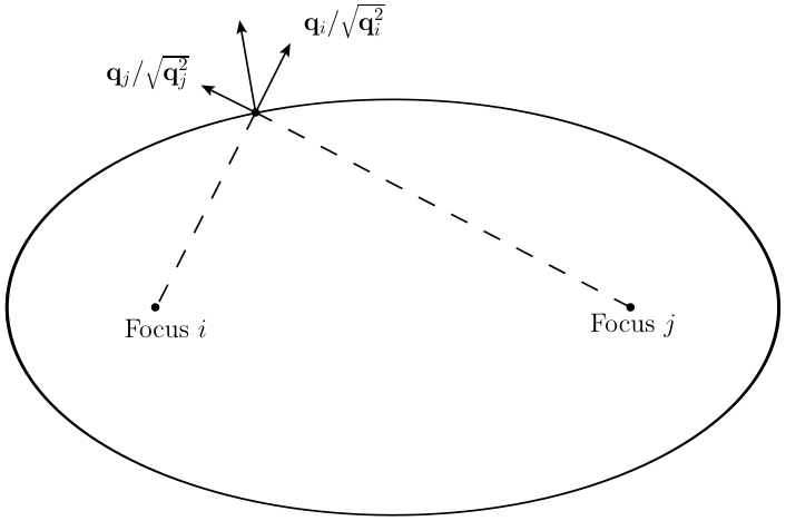
Inside the singularity ellipsoid the two vectors $\mathbf{q}_{i}/\sqrt{\mathbf{q}_{i}^{2}}$ and $\mathbf{q}_{j}/\sqrt{\mathbf{q}_{j}^{2}}$ cancel totally along the major axis of the ellipsoid. This cancellation in the vicinity of the center of the singularity ellipsoid is shown in Fig. 7. In order to be able to plot the situation, the graphs are restricted to 1+2 dimensions. Keep in mind that the imaginary part of the plotted deformation is a two component vector where each component is a function of $\ell_{x}$ and $\ell_{y}$ . Therefore, the graphs 7(a) and 7(b) indicate how far the deformation goes in the direction of the imaginary part of the $\ell_{x}$ - and $\ell_{y}$ -axis.

The suppression factor $\exp(-G_{D}^{-2}(q_{j};q_{i})/A_{ij})$ fulfills the second condition. At the position of the singularity, $G_{D}^{-2}(q_{j};q_{i})$ is 0 and thus the suppression factor reaches its maximum. Far away from the singularity, $-G_{D}^{-2}(q_{j};q_{i})$ is a large negative value and thus the exponential is close to zero. This behaviour is demonstrated in Fig. 8.

$\lambda_{ij}$ is a scaling factor analogous to $\lambda$ in Section 1. $A_{ij}$ is the width of the deformation. The indices $ij$ in $\lambda_{ij}$ and $A_{ij}$ indicate that those parameters can be chosen individually for each contribution to the deformation for optimization purposes. Then we sum over the entire group and arrive at:

\displaystyle i\boldsymbol{\kappa}=i\sum\limits_{i,j\in\text{group}}\lambda_{ij}\left(\frac{\mathbf{q}_{i}}{\sqrt{\mathbf{q}_{i}^{2}}}+\frac{\mathbf{q}_{j}}{\sqrt{\mathbf{q}_{j}^{2}}}\right)\exp\left(\frac{-G_{D}^{-2}(q_{j};q_{i})}{A_{ij}}\right)

(23)

where, of course, $i$ is the imaginary unit. Finally, we add the imaginary contribution to the loop momentum to make the deformation complete.

\displaystyle\boldsymbol{\ell}\to\boldsymbol{\ell}^{\prime}=\boldsymbol{\ell}+i\boldsymbol{\kappa}

(24)

The corresponding Jacobian can be calculated analytically.

6 Choosing the parameters

As mentioned before, the parameters $\lambda_{ij}$ and $A_{ij}$ are the scaling and the width of the deformation. Typically, $\lambda_{ij}$ is a dimensionless negative number and $A_{ij}$ a positive number of dimension $q^{4}$ ; setting all $\lambda_{ij}=0$ completely switches off the deformation.
Although they can all be chosen differently, selecting $\lambda_{ij}=\lambda=-0.5$ and $A_{ij}=A=10^{6}$ produces very good results for most of the examples that we are presenting within this thesis. As a rule of thumb, $A_{ij}\approx 10^{2}m^{4}$ where $m^{4}$ is a measure for the $\text{energy}^{4}$ of the process in consideration.

1 The scaling parameter $\lambda$

The parameter $\lambda_{ij}$ determines how far an individual contribution to the deformation goes around a pole. This is illustrated in Fig. 9, in which for the sake of clarity we restricted ourselves to $1+1$ dimensions and a deformation that consists of only one contribution.

Figure 9: The deformation at different values of

\lambda

. The dashed vertical lines mark the positions of the singularities.

From the dotted to the dashed and finally to the solid line, $\lambda_{ij}=\lambda$ has been doubled every time while keeping the width constant. Therefore, the peak of the solid curve is four times higher (lower) than the dotted one. Between $l_{x}=0$ and $l_{x}=3$ there is a region where the deformation vanishes. This is the cancelling effect of the vector part mentioned in Section 2. In 1+1 dimensions this leads to a total cancellation. It is equivalent to slicing Fig. 7 along the axis that connects the two foci of the singularity ellipse.
There is one further aspect to it which is inspired by [89]. On the one hand, we would like to choose $\lambda$ as large as possible to stay away from the singularity. One the other hand, we would like to make $\lambda$ as small as possible in order to ensure that we do not enclose other (unwanted) singularities. To escape from this dilemma, consider the on shell energy $q_{i,0}^{(+)}$ with the deformation $\boldsymbol{\ell}+i\bar{\lambda}\boldsymbol{\kappa}$ plugged in:

\displaystyle\mathbf{q}_{i,0}^{(+)}=\sqrt{-\bar{\lambda}^{2}\boldsymbol{\kappa}^{2}+2i\bar{\lambda}\boldsymbol{\kappa}\cdot\mathbf{q}_{i}+\mathbf{q}_{i}^{2}+m_{i}^{2}-i0}~.

(25)

Here we have introduced an overall factor $\bar{\lambda}$ . It scales the entire deformation as opposed to the $\lambda_{ij}$ which scale individual contributions to the deformation (see Eq. (23)).
Since $q_{i,0}^{(+)}\geq 0$ , this puts a constraint on $\bar{\lambda}$ . We set the square root to zero and solve the quadratic equation in $\bar{\lambda}$ :

\displaystyle\bar{\lambda}_{\pm}=iX_{i}\pm\sqrt{Y_{i}-X_{i}^{2}}

(26)

with

\displaystyle X_{i}

\displaystyle=\frac{\mathbf{q}_{i}\cdot\boldsymbol{\kappa}}{\boldsymbol{\kappa}^{2}},

\displaystyle Y_{i}

\displaystyle=\frac{\mathbf{q}_{i}^{2}+m_{i}^{2}}{\boldsymbol{\kappa}^{2}}

(27)

where $X_{i}\leq 0$ and $Y_{i}\geq 0$ . If $X_{i}^{2}>Y_{i}$ , the poles of $q_{i,0}^{(+)}$ lie on the imaginary $\bar{\lambda}$ -axis and the real value of $\bar{\lambda}$ may take any value. If however, $X_{i}^{2}<Y_{i}$ and $X_{i}\to 0$ we have a pole at $\bar{\lambda}=\sqrt{Y_{i}}$ . Thus we define $\bar{\lambda}$ in the following way:

\displaystyle\bar{\lambda}=\begin{cases}\frac{1}{2}\sqrt{Y_{i}}&\text{if}\quad X_{i}^{2}<Y_{i}/2,\\ \sqrt{X_{i}^{2}-\frac{Y_{i}}{4}}&\text{if}\quad Y_{i}/2<X_{i}^{2}<Y_{i},\\ 1&\text{if}\quad Y_{i}<X_{i}^{2}\end{cases}

(28)

After performing this check for every dual contribution in the deformation group, we end up with a set of “safety $\bar{\lambda}$ s” out of which we pick the smallest. Using this procedure, we make sure that our deformation does not come too close to other singularities originating from the dual delta function.

2 The width of the deformation

The parameter $A_{ij}$ determines how broad or narrow the peaks of the deformation contributions are. This is illustrated in Fig. 10. Again, to improve clarity, the plot is restricted to $1+1$ dimensions and the deformation used has only a single contribution to it.

Figure 10: The deformation at different values of

A

. The dashed vertical lines mark the positions of the singularities.

This time the width has been increased by a factor of five from the dotted to the dashed curve and another factor five from the dashed to the solid curve. The scaling parameter $\lambda$ has been kept constant.
As mentioned, setting $A_{ij}=A=10^{6}$ works fine for the majority of momentum configurations that we tested. Nonetheless, there are some cases where a bigger (or smaller) choice of width is advised to get good precision. To understand why, let us have a look at the dual propagator in its rewritten form:

\displaystyle G_{D}(q_{i};q_{j})=\frac{1}{(q_{i,0}^{(+)}+k_{ji,0})^{2}-(q_{j,0}^{(+)})^{2}}~.

(29)

We see that the inverse of the dual propagator is proportional to momentum $G_{D}^{-1}\sim q$ . In the suppression factor the inverse of the dual propagator gets squared. Hence the exponent of the suppression factor is $\sim q^{2}/A$ . In order to avoid the deformation getting to wide or too narrow, it is necessary choose the width proportional to the physical energy scale of the external momenta.

7 Numerical Results

Now we are in possession of all the necessary tools to make the numerical integration work. We have a code which runs on a desktop machine with an Intel i7 (3.4GHz) processor with 8 cores and 16 GB of RAM. Memory consumption is negligible.

1 Details on the implementation

The program is written entirely in C++ and uses the Cuba library [71] as a numerical integrator. This means it can be run on any machine on which C++ and the Cuba library are available. As input the user has to specify the number of external legs, the external momenta themselves, the internal masses and, if necessary, the parameters of the contour deformation. The momenta and masses can be read in from a text file. With regard to the numerical integrator the user can choose between Cuhre [95, 96] and VEGAS and give the desired number of evaluations. At this stage, the program is ready to be compiled and executed. Schematically speaking, it performs the following steps:

1.

Read in momenta and masses.
2.

Check where ellipsoid singularities occur.
3.

Check where hyperboloid singularities occur and group the dual contributions accordingly.
4.

Call the integrator, taking into account the number of external legs as well as the results from the previous steps.

We use MATHEMATICA 8.0 [97] to generate randomized momenta and masses and LoopTools 2.10 [98] to produce reference values for comparison. The goal is to scan as much of the phase-space as possible to make sure the program works properly in all regions. The momenta of all the example points and scans of the following sections are collected in Appendix 11.
We see two main paths along which the complexity of the calculation grows.

1.
Increasing the number of external legs. In general, going from $n\to n+1$ legs means for the Duality:
- •
  
  One extra dual contribution.
- •
  
  Since each dual contribution does consist of one more dual propagator, there are much more possibilities for ellipsoid singularities to occur. Thus the deformation picks up more contributions.
Therefore, we investigate multi-leg scalar integrals up to the pentagon level in this chapter.
2.

The presence of tensor numerators. Having tensors of increasing rank in the numerator will render the function to be integrated more complex. We address tensor integrals in Chapter 7 although it does not affect the singular behaviour of the integral.

Our setup is such that we run points asking for a fixed number of evaluations. Then we modify the parameters of the deformation for best results.²² 2 Part of the results which we are going to show in the following will be published in a forthcoming paper [3].

2 Scalar Triangle

We consider first infrared finite triangle (three external legs) scalar integrals. Momentum configurations that do not need deformation (i.e. whose loop integral is purely real) are integrated in about $0.15$ seconds with a precision of at least 4 digits. $5\cdot 10^{4}$ evaluations are sufficient to achieve this result.

	Point 1	Point 1 Error	Point 2	Point 2 Error
LoopTools	-5.85694E-5	0	-3.39656E-7	0
Loop–Tree Duality	-5.85685E-5	2.4E-9	-3.39688E-7	5.3E-11

Table 1: Example for two non-deformation phase-space points. Since there is no deformation, all values are purely real.

Point of Table 1 has all internal masses equal while Point has three different internal masses. Momenta and masses were chosen randomly between $-100$ and $+100$ . This even allows for unphysical momentum configurations, but at this stage we want to test stability and precision regardless of whether we are in the physical region or not. For example, although Triangle represents a situation that is not realized in nature, it is computed without any problems. From the program’s point of view there is no difference; the internal masses are mere parameters.
For momentum configurations that require deformation the function to integrate is more complicated, hence we have to evaluate it more often. With $10^{6}$ iterations, the calculation time increases to around $2.5$ seconds. Four digits of precision are achievable by optimizing the parameters of the deformation.

	Real Part	Real Error	Imaginary Part	Imaginary Error
LoopTools P.3	5.37305E-4	0	-6.68103E-4	0
Loop–Tree Duality P.3	5.37307E-4	8.6E-9	-6.68103E-4	8.6E-9
LoopTools P.4	-5.61370E-7	0	-1.01665E-6	0
Loop–Tree Duality P.4	-5.61371E-7	7.2E-10	-1.01666E-6	7.2E-10

Table 2: Example for two phase-space point that need deformation. With a deformation applied, the results are complex.

Similar to the non-deformation points before, Point of Table 2 has all internal masses equal whereas in Point all three of them have different values. Regardless of kinematics, the Loop–Tree Duality is capable of producing accurate results in both situations.

Fig. 11 gives an additional view on a triangle example phase-space point: Each of the cubes in the first line represents one dual contribution. Drawn are the ellipsoid (violet surfaces) and hyperboloid (orange surfaces) singularities in loop-momentum space. The blue dots are the positions of the foci of the on-shell hyperboloids, i.e. $-\mathbf{k}_{i},\,\,\,i\in\{1,2,3\}$ . In the second line we have the singularity scheme. This means each line of the singularity scheme corresponds to one box.

Another important check is the scan around threshold. This region is usually numerically unstable. The Loop–Tree Duality excels here, because the algorithm does not have to do extra work. In Fig. 12 all internal masses are equal, i.e. $m_{i}=m$ , $i\in\{1,2,3\}$ , and the center-of-mass energy $s$ was kept constant while the mass $m$ was varied. As you can see from the plots, there is no drop in precision around threshold. Calculation time remains constant, as well.

3 Scalar Boxes

We repeated the analysis for the box (four external legs) case. The main difference is that now there are four dual contributions with three dual propagators each.
To get good precision, we chose to evaluate boxes that need deformation for $4\cdot 10^{6}$ times, while the number of evaluations for non-deformation phase-space points was kept at $5\cdot 10^{4}$ evaluations, the same as in the triangle case. This is reflected in the program runtimes. Deformation points take 16 seconds, non-deformation points take about 0.25 seconds, respectively.
While it is practically guaranteed to get the non-deformation points with good precision, the quality of results depends on the proper choice of parameters for points with deformation. Therefore, we focus our attention towards such points by giving many more examples for them.
A very good method to do so is to perform a mass-scan as we already did in the triangle case. From Fig. 14 to Fig. 16 we present scans for the following momentum configurations:

•

All internal masses equal. The center-of-mass energy $s$ is kept constant while the mass is varied. This is shown in Fig. 14.
•

Two adjacent internal masses equal and the two opposing masses equal, i.e. $m_{1}=m_{2}$ and $m_{3}=m_{4}$ . $m_{1}$ and therefore also $m_{2}$ is varied, the other momenta and masses are kept constant. This is shown in Fig. 15.
•

Scan in which the Mandelstam variable $t$ is varied. This is realized by varying $p_{3}$ while keeping $p_{3}^{2}$ constant. Of course, due to momentum conservation, this involves $p_{4}^{2}=(p_{1}+p_{2}+p_{3})^{2}$ not being constant. This is shown in Fig. 16.

Concrete values for each of those situations are found in Table 3.
The scans show how the program performs in certain slices of the phase space. This is important because we want the program to be generically applicable to any momentum configuration. From the plots and tables, you can see that the program deals well with all kinds of boxes, even when many different kinematical scales are involved.

Point and of Table 3 correspond to a momentum configuration, in which all four internal masses are equal. In Point and all masses are different. In Point two adjacent internal lines have equal masses as well as the two opposing ones. Point represents a situation in which opposite lines have equal masses.

	Point 5	Point 5 Error	Point 6	Point 6 Error
LoopTools	2.15339E-13	0	1.39199E-11	0
Loop–Tree Duality	2.15319E-13	5.2E-17	1.39199E-11	6.3E-16

(a) Two non-deformation phase-space points.

	Real Part	Real Error	Imaginary Part	Imaginary Error
LoopTools P.7	-2.38766E-10	0	-3.03080E-10	0
Loop–Tree Duality P.7	-2.38798E-10	8.2E-13	-3.03084E-10	8.2E-13
LoopTools P.8	-4.27118E-11	0	4.49304E-11	0
Loop–Tree Duality P.8	-4.27127E-11	5.3E-14	4.49301E-11	5.3E-14
LoopTools P.9	6.43041E-11	0	1.61607E-10	0
Loop–Tree Duality P.9	6.43045E-11	8.4E-15	1.61607E-10	8.4E-15
LoopTools P.10	-4.34528E-11	0	3.99020E-11	0
Loop–Tree Duality P.10	-4.34526E-11	3.5E-14	3.99014E-11	3.5E-14

(b) Four phase-space points with different kinematics that need deformation.

Table 3: Examples for boxes with and without deformation.

Similar to the triangle case, Fig. 13 shows the singularities in loop three-momentum space. It becomes immediatly obvious that, only by going to box graphs, the level of complexity has grown substantially. Because the hyperboloid singularities couple dual contributions together, an individual contribution receives a much more complicated deformation.

In Fig. 13, the dots give the locations of the foci $-\mathbf{k}_{i}$ , the surfaces are ellipsoid and hyperboloid singularities. Note how the hyperboloids always appear pairwisely across the dual contributions.

Figure 14: Mass-scan of a box integral. The red curve is LoopTools, the blue points are the Loop–Tree Duality.

In Fig. 14, two thresholds are passed at $2m/\sqrt{s}=0.65$ and $1$ . From right to left, the number of ellipsoid singularities grows by one after each threshold from one to three.

Figure 15: Mass-scan of a box integral. The red curve is LoopTools, the blue points are the Loop–Tree Duality.

In Fig. 15, one threshold is crossed at $2m_{1}/\sqrt{s}\approx 0.65$ . From right to left the number of ellipsoid singularities goes from one to two.

Figure 16:

t

-scan of a box integral. The red curve is LoopTools, the blue points are the Loop–Tree Duality.

In Fig. 16, the Mandelstam variable $t$ is being varied. Two thresholds are passed, one at $t\approx 10^{4}$ and one at $t\approx 150\cdot 10^{4}$ . From left to right, the number of ellipsoid singularities increases by one after each crossing of a threshold from zero to two.

4 Scalar Pentagons

After the evaluation of triangles and boxes, the next step is to check pentagon (five external legs) graphs. Complexity grows once more, which means:

•

A dual integral now consists of five dual contributions.
•

Each dual contribution contains one additional ( $=$ four in total) dual propagator.

Therefore, we had to increase the number of evaluations: Non-deformation points are evaluated $10^{5}$ times which takes approximately $0.5$ seconds. Points with deformation demand $5\cdot 10^{6}$ evaluations to maintain the level of precision of the triangles and boxes. This results in an average calculation time of 28 seconds. This enhanced complexity is especially well-illustrated by the following Figure in which the singularities of the different dual contributions are plotted in loop-momentum space:

Again, dots are foci of the on-shell hyperboloids, surfaces are ellipsoid and hyperboloid singularities. From the singularity scheme we can read off that all five dual contributions are coupled together due to the interaction of the hyperboloids.

	Point 11	Point 11 Error	Point 12	Point 12 Error
LoopTools	-1.24025E-13	0	-1.48356E-14	0
Loop–Tree Duality	-1.24027E-13	1.6E-17	-1.48345E-14	1.1E-17

(a) Two non-deformation phase-space points.

	Real Part	Real Error	Imaginary Part	Imaginary Error
LoopTools P.13	1.02350E-11	0	1.40382E-11	0
Loop–Tree Duality P.13	1.02353E-11	1.0E-16	1.40385E-11	1.0E-16
LoopTools P.14	7.46345E-15	0	-9.13484E-15	0
Loop–Tree Duality P.14	7.46309E-15	6.1E-18	-9.13444E-15	6.1E-18
LoopTools P.15	6.89836E-15	0	2.14893E-15	0
Loop–Tree Duality P.15	6.89848E-15	6.5E-18	2.14894E-15	6.5E-18

(b) Three phase-space points that need deformation.

Table 4: Examples for pentagons with and without deformation.

Table 4 displays a collection of pentagon sample results for different kinematical configurations. In Points and all internal masses are equal; in Point they are all distinct from each other and in Point we have $m_{1}=m_{2}=m_{3}\neq m_{4}=m_{5}$ . Again, the Loop-Tree Duality shows its robustness by producing accurate results regardless of the kinematical situation. This statement is further supported by various scans we performed:

•

All internal masses equal. The center-of-mass energy $s$ is kept constant while the mass gets varied. This is shown in Fig. 18.
•

All five internal masses different. Mass $m_{1}$ gets varied, the rest is kept constant. This is shown in Fig. 19.
•

Scan in which the center-of-mass energy $s$ is varied. This is realized by varying $p_{1}$ . Of course, due to momentum conservation, this involves $p_{4}^{2}=(p_{1}+p_{2}+p_{3})^{2}$ not being constant. This is shown in Fig. 20.

From the plots, you can see that the Loop-Tree Duality is able to achieve good precision for pentagons as well. Even situations in which many ellipsoid singularities are involved, are handled well by the program. For example, the number of ellipsoid singularities in Figure 18 increases from two to five when going from right to left.

Figure 18: Mass-scan of a pentagon integral. The red curve is LoopTools, the blue points are the Loop–Tree Duality.

Three thresholds are passed in this scan. From right to left, we start at two ellipsoid singularities and arrive at five.

Figure 19: Mass-scan of a pentagon integral. The red curve is LoopTools, the blue points are the Loop–Tree Duality.

One threshold is crossed at $2m_{1}/\sqrt{s}\approx$ 0.2. From right to left, the number of ellipsoid singularities increases from five to six.

Figure 20: Energy-scan of a pentagon integral. The red curve is LoopTools, the blue points are the Loop–Tree Duality.

In this scan, we pass three thresholds at $s\approx-8.5\cdot 10^{3},-13.5\cdot 10^{3}$ and $-21\cdot 10^{3}$ which divide the graph into four zones. From right to left, we start with zero ellipsoid singularities in the first zone, then we have one in the second zone, two in the third zone and finally one in the last zone.

Chapter 7 Tensor Integrals

Up to this point, we have shown that the Loop–Tree Duality is capable of dealing with all kinds of kinematical configurations. The only constraint that we have made was to limit ourselves to scalar integrals. In Chapter 2, we argued that the inclusion of numerators different from 1 should not be an issue for the Loop–Tree Duality because it acts only on the denominator of the loop integral. Hence, in this chapter, we are going to relieve this restriction and repeat some of the analysis of the previous chapter with tensor integrals. Additionally, we are going one step further by calculating even hexagons, which are usually tough to compute, but from the perspective of LTD are a straightforward generalization.

1 The influence of numerators

To start off, we restate the Duality Theorem for scalar integrals (cf. Eq. (3)):

\displaystyle L^{(1)}(p_{1},p_{2},\dots,p_{N})\quad=\quad-\sum_{i\in\alpha_{1}}\,\int_{\ell}\;{\widetilde{\delta}}(q_{i})\,\prod_{\begin{subarray}{c}j\in\alpha_{1}\\ j\neq i\end{subarray}}\,G_{D}(q_{i};q_{j})~,

(1)

where

G_{D}(q_{i};q_{j})=\frac{1}{q_{j}^{2}-m_{j}^{2}-i0\,\eta(q_{j}-q_{i})}~.

(2)

If our one-loop integral features a non-trivial numerator $\mathcal{N}(\ell,\{p_{i}\})$ . Then, the Loop–Tree Duality Theorem takes the form

\displaystyle L^{(1)}(p_{1},p_{2},\dots,p_{N})\quad=\quad-\sum_{i\in\alpha_{1}}\,\int_{\ell}\;{\widetilde{\delta}}(q_{i})\,\prod_{\begin{subarray}{c}j\in\alpha 1\\ j\neq i\end{subarray}}\,G_{D}(q_{i};q_{j})\mathcal{N}(\ell,\{p_{i}\})~.

(3)

While the numerator is formally left unchanged, there actually is a practical impact. The presence of the dual delta function demands $q_{i,0}^{(+)}=\sqrt{\mathbf{q}_{i}^{2}+m_{i}^{2}}$ which is equivalent to having the energy component of the loop-momentum forced to

\displaystyle\ell_{0}=-k_{i,0}+\sqrt{\mathbf{q}_{i}^{2}+m_{i}^{2}}~.

(4)

In other words, whenever we perform a single cut of a Feynman graph, the numerator has to be evaluated at the position of the cut which is fixed by the dual delta function. As a direct consequence, the numerator takes a different form in each dual contribution.

Another important aspect to take into consideration is the cancellation of singularities among dual contributions. In Section 2, we argued that numerators do not spoil the cancellation of the hyperboloid singularities. Here, we would like to make explicitly show why. A typical numerator is a product of scalar products of the form “loop-momentum contracted with external momentum”: $\ell\cdot p_{k}$ . Let us see what happens to a single factor when it hits the singularity. Note first, that the hyperboloid singularity is given by Eq. (8) which we rewrite in the more suitable form

\displaystyle q_{i,0}^{(+)}-k_{i,0}=q_{j,0}^{(+)}-k_{j,0}~.

(5)

Using Eq. (4), the loop-momentum $\ell$ contracted with some external momentum $p_{k}$ is:

	$\displaystyle\ell\cdot p_{k}\,\|_{\text{i-th cut}}$	$\displaystyle=(-k_{i}+q_{i,0}^{(+)})p_{k,0}-\boldsymbol{\ell}\cdot\mathbf{p}_{k}$
		$\displaystyle=(-k_{j}+q_{j,0}^{(+)})p_{k,0}-\boldsymbol{\ell}\cdot\mathbf{p}_{k}=\ell\cdot p_{k}\,\|_{\text{j-th cut}}$		(6)

where we have used Eq. (5) for the first equality on the second line of Eq. (6). It means that the numerators of two dual contributions $i$ and $j$ take the same value at their common pole, thus leaving the cancellation of hyperboloid singularities intact. This is an important property to take advantage of, because it allows us to straightforwardly apply the Loop–Tree-Duality to such diagrams without any additional effort.

1 An illustrative example

To make things even more explicit, consider the following simple example. We take the triangle integral of Section 2 and give it the numerator $\mathcal{N}(\ell,p_{1},p_{2})=\ell\cdot p_{1}$ :

\displaystyle I=\int_{\ell}\,\ell\cdot p_{1}\,\prod\limits_{i=1}^{3}G_{F}(q_{i})

(7)

$p_{1},p_{2}$ and $p_{3}=-p_{1}-p_{2}$ are the external momenta. Since we are dealing with a triangle, obviously $N=3$ . Consequently, the Loop–Tree Duality translates the Feynman integral into three dual contributions.

$\displaystyle I=$	$\displaystyle\int_{\ell}{\widetilde{\delta}}(q_{1})G_{D}(q_{1};q_{2})G_{D}(q_{1};q_{3})\,\ell\cdot p_{1}$
$\displaystyle+$	$\displaystyle\int_{\ell}G_{D}(q_{2};q_{1}){\widetilde{\delta}}(q_{2})G_{D}(q_{2};q_{3})\,\ell\cdot p_{1}$
$\displaystyle+$	$\displaystyle\int_{\ell}G_{D}(q_{3};q_{1})G_{D}(q_{3};q_{2}){\widetilde{\delta}}(q_{3})\,\ell\cdot p_{1}$	(8)

This time, we investigate how the numerator affects the calculus. The dual delta functions of the different contributions fix the energy component of the numerators to different values. Hence the scalar product becomes

$\displaystyle\ell\cdot p_{1}$	$\displaystyle\to(-p_{1,0}+\sqrt{(\boldsymbol{\ell}+\mathbf{p}_{1})^{2}+m_{1}^{2}})\,p_{1,0}-\boldsymbol{\ell}\cdot\mathbf{p}_{1}$	first contribution
$\displaystyle\ell\cdot p_{1}$	$\displaystyle\to(-p_{1,0}-p_{2,0}+\sqrt{(\boldsymbol{\ell}+\mathbf{p}_{1}+\mathbf{p}_{2})^{2}+m_{2}^{2}})\,p_{1,0}-\boldsymbol{\ell}\cdot\mathbf{p}_{1}$	second contribution
$\displaystyle\ell\cdot p_{1}$	$\displaystyle\to\sqrt{\boldsymbol{\ell}^{2}+m_{3}^{2}}\,p_{1,0}-\boldsymbol{\ell}\cdot\mathbf{p}_{1}$	third contribution	(9)

This means, that finally we will arrive at with three dual contributions similar to the ones of Eq. (70).

In the next sections, we present the results for multi-leg tensor integrals. We only consider IR- and UV-finite diagrams. The explicit momenta of all the points and scans presented within this chapter are found in Appendix 11.

2 Tensor Triangles

In Chapter 6, we convinced ourselves that the Loop–Tree Duality can produce accurate results for scalar one–loop integrals independent of the kinematical configuration. Now, we focus on checking various different numerator functions within a similar analysis.
We start with infrared-finite one–loop triangle graphs. The simplest non-trivial numerator function possible is the loop-momentum $\ell$ contracted with one of the external momenta $p_{1}$ or $p_{2}$ , i.e. $\ell\cdot p_{1}$ or $\ell\cdot p_{2}$ . Since we are limiting our discussion to UV-finite graphs, these are the only possible numerators at the triangle level.
The number of evaluations per phase-space point is the same as in the scalar case; this means $5\cdot 10^{4}$ evaluations for non-deformation points and $10^{6}$ evaluations for phase-space points with deformation. Due to the presence of numerators, the integrand function is a bit more complex. Hence the calculation time, compared to scalar triangles increases from 2.5 seconds to 3.5 seconds for deformation-points. For non-deformation points there is hardly any measurable difference, i.e. they stay at around 0.15 seconds
A compilation examples is shown in Table 1. Points and correspond to kinematical situations in which all internal masses are equal and the numerator is $\ell\cdot p_{2}$ , whereas Points and have all internal masses are different from each other and numerator $\ell\cdot p_{1}$ .

	Point 16	Point 16 Error	Point 17	Point 17 Error
LoopTools	-1.07284E-2	0	-1.59964E-3	0
Loop–Tree Duality	-1.07281E-2	5.4E-6	-1.59985E-3	6.6E-7

(a) Two non-deformation phase-space points.

	Real Part	Real Error	Imaginary Part	Imaginary Error
LoopTools P.18	-2.64773E-3	0	1.37469E-2	0
Loop–Tree Duality P.18	-2.64726E-3	5.5E-6	1.37448E-2	5.5E-6
LoopTools P.19	-1.19501E-2	0	1.35834E-3	0
Loop–Tree Duality P.19	-1.19511E-2	3.6E-5	1.35859E-3	3.6E-5

(b) Two phase-space points that need deformation.

Table 1: Examples for triangles involving numerators, with and without deformation.

In the triangle mass-scan of Fig. 1, we varied the mass in the same way as we did in the previous chapter. Three thresholds are passed at $2m/\sqrt{s}\approx 0.15$ , 0.45 and 1.

Figure 1: Mass-scan of a triangle with numerator

\ell\cdot p_{3}

. The red curve is LoopTools, the blue points are the Loop–Tree Duality.

3 Tensor Boxes

Again, we repeat the analysis of the triangles at the box-level. We only want to deal with UV-finite diagrams, thus tensors up to rank three are allowed in the numerator. Since having a rank-one tensor is quite similar to the triangle case, we will focus on rank two and rank three situations in order to have a more challenging test for the program.
We use the same number of evaluations as we did for scalars, this means $4\cdot 10^{6}$ evaluations for deformation points and $5\cdot 10^{4}$ evaluations for points that do not need deformation. As far as deformation points are concerned, calculation times differ according to the rank of the tensor function in the numerator. Their general order of magnitude is around 20 seconds, the span between a rank zero and a rank three tensor amounts to 8 seconds. Non-deformation points take about 0.25 seconds, almost independently of the rank of the numerator function.

	Point 20	Point 20 Error	Point 21	Point 21 Error
LoopTools	-3.42913E-4	0	9.64909E+0	0
Loop–Tree Duality	-3.42905E-4	5.9E-8	9.64924E+0	4.6E-3

(a) Two non-deformation phase-space points.

	Real Part	Real Error	Imaginary Part	Imaginary Error
LoopTools P.22	1.33032E-3	0	-1.07780E-3	0
Loop–Tree Duality P.22	1.33033E-3	5.6E-7	-1.07779E-3	5.6E-7
LoopTools P.23	-2.15448E+2	0	-1.10792E+2	0
Loop–Tree Duality P.23	-2.15451E+2	8.7E-2	-1.10789E+2	8.7E-2

(b) Two phase-space points that need deformation.

Table 2: Examples for boxes involving numerators of tensor rank two and three, with and without deformation.

In Table 2, Points and are boxes with all internal masses equal and numerator $\ell\cdot p_{1}\times\ell\cdot p_{2}$ . Points and represent situations in which all internal masses are different and the numerator has the form $\ell\cdot p_{1}\times\ell\cdot p_{3}\times\ell\cdot p_{4}$ .

We also did a scan of the Mandelstam variable $t$ , see Fig. 2, for which we took a box with three scalar products in the numerator, $\ell\cdot p_{1}\times\ell\cdot p_{2}\times\ell\cdot p_{3}$ , and varied $p_{3}$ while keeping $p_{3}^{2}$ constant. Since $p_{3}$ also appears in the numerator, both numerator and denominator are affected by this scan.

Figure 2: Scan of the region around threshold. The red curve is LoopTools the blue points are the Loop–Tree Duality.

4 Tensor Pentagons

Next, we investigate pentagon tensor integrals at the one–loop level with numerators up to rank three. The number of evaluations is chosen to be the same as in the scalar case, i.e. $10^{5}$ times for non-deformation and $5\cdot 10^{6}$ times for phase-space points that require deformation. This results in calculation times of 0.7 seconds and 33 seconds, respectively. The runtime difference between a point with a numerator of rank zero and rank three is negligible for non-deformation points and about 10 seconds for deformation points.
Table 3 shows a selection of sample points. Point and feature the rank two numerator $\ell\cdot p_{3}\times\ell\cdot p_{4}$ while Point and have the numerator $\ell\cdot p_{3}\times\ell\cdot p_{4}\times\ell\cdot p_{5}$ . In all points all internal masses are equal. At first glance, Point seems to be weaker but it actually contains six ellipsoid singularities whereas the other points usually have two to three. We include this point to demonstrate that the program holds well together even under such challenging circumstances.

	Point 24	Point 24 Error	Point 25	Point 25 Error
LoopTools	-1.86472E-8	0	1.74828E-3	0
Loop–Tree Duality	-1.86462E-8	2.6E-12	1.74808E-3	2.8E-7

(a) Two non-deformation phase-space points.

	Real Part	Real Error	Imaginary Part	Imaginary Error
LoopTools P. 26	-1.68298E-6	0	1.98303E-6	0
Loop–Tree Duality P. 26	-1.68298E-6	7.4E-10	1.98299E-6	7.4E-10
LoopTools P. 27	-8.34718E-2	0	1.10217E-2	0
Loop–Tree Duality P. 27	-8.34829E-2	7.5E-5	1.10119E-2	7.5E-5

(b) Two phase-space points which need deformation.

Table 3: Examples for pentagons involving numerators of tensor rank two and three, with and without deformation.

We also performed several scans; a sample is presented in Figure 3. In that scan, similarly to what we have done with scalar pentagons, we varied $p_{1}$ and thus the center-of-mass energy $s=(p_{1}+p_{2})$ . The corresponding numerator function is $\ell\cdot p_{1}\times\ell\cdot p_{2}\times\ell\cdot p_{3}$ , which means that both numerator and denominator take part in the scan. From the plot, we can see that the Loop-Tree Duality is able to pass this challenging test.

Figure 3: Scan of the region around threshold. The red curve is LoopTools, the blue points are the Loop–Tree Duality.

5 Tensor Hexagons

We also analysed hexagon (six external legs) tensor integrals, for which we raised the number of evaluations for non-deformation points to $10^{6}$ and for deformation points to $8\cdot 10^{6}$ . The corresponding calculation times are 8 and 75 seconds, respectively. Since we evaluate non-deformation points ten times more compared to pentagons, the different numerators have a measurable impact on the calculation time. The difference between rank zero and rank three is 6 seconds and 15 seconds for deformation points.
LoopTools can provide reference values only up to pentagons. Instead, we used the program SecDec version 3 [38] for comparison.
Again, we present a selection of sample points in Table 4. Point and feature the rank-one numerator $\ell\cdot p_{1}$ , in the former all internal masses are different and in the latter they are all equal. Point has six distinct internal masses and the numerator function $\ell\cdot p_{2}\times\ell\cdot p_{4}\times\ell\cdot p_{6}$ , Point possesses the numerator $\ell\cdot p_{2}\times\ell\cdot p_{5}$ and six different masses, as well. Finally, in Point , which exhibits the numerator $\ell\cdot p_{4}\times\ell\cdot p_{5}\times\ell\cdot p_{6}$ , all momenta are distinct form each other.

	Point 28	Point 28 Error	Point 29	Point 29 Error
SecDec	-1.21585E-15	1.2E-19	4.46117E-9	3.7E-13
Loop–Tree Duality	-1.21552E-15	3.5E-18	4.46136E-9	2.6E-15

(a) Two non-deformation phase-space points.

	Real Part	Real Error	Imaginary Part	Imaginary Error
SecDec P. 30	1.01359E-15	2.3E-19	2.68657E-15	2.6E-19
Loop–Tree Duality P. 30	1.01345E-15	1.3E-18	2.68633E-15	1.3E-18
SecDec P. 31	2.45315E-12	2.4E-16	-2.06087E-12	2.0E-16
Loop–Tree Duality P. 31	2.45273E-12	7.3E-15	-2.06202E-12	7.3E-15
SecDec P. 32	-2.07531E-6	1.9E-10	6.97158E-7	5.6E-11
Loop–Tree Duality P. 32	-2.07526E-6	7.5E-13	6.97192E-7	7.5E-13

(b) Two phase-space points that need deformation.

Table 4: Examples for pentagons involving numerators of tensor rank two and three, with and without deformation.

Chapter 8 Summary and Future Work

1 Summary

One of the main difficulties in calculating scattering amplitudes at NLO and higher is the cancellation of infrared singularities among real and virtual corrections. The Loop–Tree Duality aims to solve that problem by recasting the virtual corrections in a form which closely resembles the real ones. This appealing property motivates the idea of combining the two, thus treating them simultaneously in a common Monte Carlo event generator.
Initially the LTD was introduced for scalar one–loop integrals [48] and in later works its applicability has been expanded by a large margin via a systematic procedure has been established to calculate Feynman graphs with an arbitrary number of loops [49]. In Chapter 4 and in [1] we have shown how to deal with loop integrals involving higher order poles. Instead of applying the Residue Theorem for higher order poles, using Integration By Parts techniques reduced the integrals featuring such poles to integrals with simple poles. After that we could go ahead and straightforwardly apply the known formulae. At that point, the major theoretical questions were answered and the important was to check the efficiency of the method. To that direction, as a preparatory step (Chapter 5 and [2]), we investigated the singularities of the dual contributions and found a partial cancellation of singularities among contributions happening at the integrand level. In the case of massless diagrams, we were able to show that the infrared singularities are confined to a finite region of loop-momentum space which can then be mapped to the real corrections. With this information at hand, we did a numerical implementation of the Loop–Tree Duality in the form of a computer program written in C++. Being a first step towards the combined treatment, the program calculated one-loop integrals. Due to the partial cancellation of singularities, we only had to deal with singularities of the ellipsoid type. We dealt with the ellipsoid singularities by contour deformation. Still, the hyperboloid singularities affected the way we deformed: In order to keep the cancellations intact, we grouped dual contributions featuring the same hyperboloid singularities together. Then, we employed a contour deformation that accounted for all the ellipsoid singularities of the entire group. This contour deformation was constructed to respect the $i0$ -prescription of the propagators and fall rapidly to 0 where it was not needed so that the value of the overall integral would not be altered. Since dual integrals are three–dimensional, we only had to deform in loop three-momentum space. As integrators we used Cuhre and VEGAS from the Cuba library. This setup has proven to be successful. We were able to calculate (UV- and IR-finite) scalar with good precision. This has been illustrated by showing individual points as well as several scans through the phase space, in which we picked one mass or momentum to be varied while the other ones were kept constant. In Chapter 7 we also demonstrated that the Loop-Tree Duality deals equally well with tensor integrals (numerators different from 1) up to rank three.
The numerical implementation is still in an early state. Neverthelss, the wide range of checks we have performed proves the potential of the method. In particular, the implementation works well independently from the number of kinematical scales (bilinears, trilinears, different masses) involved or whether a phase space point is in the vicinity of a threshold or not.

2 Future Work

Having shown that the Loop–Tree Duality method works and is efficient, the next step will be to address any issue the code might run into. Furthermore we would like to provide a systematical way to choose the parameters $\lambda$ and the width for optimal results. We also aim to try the LTD for a real, physical process (i.e. not a toy model), for example the six- or eight-photon amplitude. To that end, we will move towards treating a case where we combine the real and virtual corrections. The goal is to have a highly automated program which calculates the entire cross-section at the one-loop level. Finally, the next step in our list is to implement the LTD for two-loop amplitudes. This is quite an extensive list, but with the presented work we have laid a good basis.

Chapter 9 Duality Nomenclature

•

Loop–Tree Duality:
The Loop–Tree Duality (in short: Duality) is a Feynman integral transformation that maps loop integrals to a sum of phase-space (tree–level) integrals. Within the conventions of Chapter 2, the Loop–Tree Duality at one-loop level looks like:

\displaystyle\int_{\ell}\,\prod\limits_{i=1}^{N}\,G_{F}(q_{i})\quad\longrightarrow\quad-\sum\limits_{i=1}^{N}\,\int_{\ell}\;{\widetilde{\delta}}(q_{i})\,\prod_{\begin{subarray}{c}j=1\\ j\neq i\end{subarray}}^{N}\,G_{D}(q_{i};q_{j})

(1)

This transformation is achieved by performing the integration over the energy component of the loop integral. The resulting integration runs only over the loop three-momentum and is very similar to the real radiation corrections. Thus, it encourages the idea of combining the two, treating them simultaneously in a common Monte Carlo event generator.
Each summand is called dual contribution and is constructed according to a special pattern: One of the internal lines gets on-shell, i.e. it is replaced by a dual delta function, while all the other (non-cut) Feynman propagators are promoted to dual propagators. This procedure is repeated for every internal line once and the results are added together to yield the dual integral.

•

Dual delta function:
The dual delta function ${\widetilde{\delta}}(q_{i})$ is the delta function that appears after applying the Loop–Tree Duality:

{\widetilde{\delta}}(q_{i})\equiv 2\pi\,i\,\theta(q_{i,0})\,\delta(q_{i}^{2}-m_{i}^{2})=2\pi\,i\,\delta_{+}(q_{i}^{2}-m_{i}^{2})

It serves several purposes. Formally it is there (cf. Eq. (1)) to indicate that the energy integration has already been carried out, leaving an integral over the loop three-momentum only. It fixes the $\ell_{0}$ -component to a certain value determined by the argument of the delta function. The theta function, which is included in the dual delta function, ensures that the positive energy solution gets picked from the argument of the dual delta function.

•

Dual propagator:
Applying the Loop–Tree Duality involves converting all Feynman propagators to dual propagators, except the cut one. There are two representations of the dual propagator,

{\widetilde{\delta}}(q_{i})G_{D}(q_{i};q_{j})=\frac{{\widetilde{\delta}}(q_{i})}{q_{j}^{2}-m_{j}^{2}-i0\,\eta\cdot k_{ji}}\quad\text{and}\quad G_{D}(q_{i};q_{j})=\frac{1}{(q_{i,0}^{(+)}+k_{ji,0})^{2}-(q_{j,0}^{(+)})^{2}}~,

(2)

where

q_{i,0}^{(+)}=\sqrt{\mathbf{q}_{i}^{2}+m_{i}^{2}-i0}~.

(3)

The main difference between a dual propagator and a Feynman propagator is the $i0$ -prescription. The Feynman propagator depends on the loop four-momentum as opposed to the dual propagator which depends on the loop three-momentum.
The $i0$ -prescription indicates which way to go around the singularities when integrating. Since the integration of the energy component has already been carried out, the dual propagator can only depend on the loop three-momentum and the $i0$ -prescription gets modified (for details on how and why this happens, see Section 3). As a direct consequence, the new dual prescription is merely a way of bookkeeping on how to go around singularities in loop three-momentum space.
The form on the left of Eq. (2) is a natural result of the derivation of the Loop–Tree Duality, the form on the right is a little more suited for numerical implementations.

•

Dual prescription:
The modified $i0$ -prescription of the dual propagator is called dual prescription. The dual prescription of the dual propagator $G_{D}(q_{i};q_{j})$ has the form

$\displaystyle-i0\eta\cdot k_{ji}~,$ (4)

where $\eta$ is a future-like four-vector, $\eta^{2}\geq 0,\eta_{0}>0$ . Typically, $\eta$ is chosen to be $(1,0,0,0)$ . In general, $\eta$ depends on the choice of the coordinate frame. Nonetheless, once all dual contributions have been added together, $\eta$ cancels out. In other words dual integrals are independent from the choice of $\eta$ whereas individual dual contributions do depend on it. At one–loop, the vector $k_{ji}=q_{j}-q_{i}$ does not depend on the loop momentum and determines the sign of the dual prescription.
•

Dual contribution:
A dual contribution is one individual summand of the sum in Eq. (1),

$\displaystyle\int_{\ell}\;{\widetilde{\delta}}(q_{i})\,\prod_{\begin{subarray}{c}j=1\\ j\neq i\end{subarray}}^{N}\,G_{D}(q_{i};q_{j})~.$ (5)

It represents one single cut of a one-loop diagram. The cut line gets replaced by a dual delta function, the Feynman propagators of all other internal lines are promoted to dual propagators. This is demonstrated explicitly in Section 2.
Loop–Tree Duality converts a one-loop integral with $N$ external legs into a sum of $N$ dual contributions. While the original one-loop integral runs over the loop four-momentum, the integrations of the dual contributions are only three-dimensional thus simplifying the calculation.
Individual dual contributions can feature singularities (hyperboloid singularities, cf. Section 3) that partially disappear once all dual contributions are combined.

•

Dual integral:
The dual integral is the end result obtained by applying the Loop–Tree Duality to a one-loop integral:

\displaystyle-\sum\limits_{i=1}^{N}\,\int_{\ell}\;{\widetilde{\delta}}(q_{i})\,\prod_{\begin{subarray}{c}j=1\\ j\neq i\end{subarray}}^{N}\,G_{D}(q_{i};q_{j})

(6)

It features a couple of appealing properties: Since the $\ell_{0}$ -integration has already been performed, the resulting dual integral only involves a three-dimensional integration. In fact, it resembles the form of the real corrections. Therefore, the Loop–Tree Duality aims towards a combined treatment of loop and tree contributions.

Chapter 10 Proof of the Reduction of Eq. (18)

Here we solve the system of equations, explicitly, to arrive at Eq. (18). We note that we are not aiming for a full reduction to a set of master integrals but rather to reduce the multiple poles to single poles. Therefore, any integral which has single propagators is to be considered known.

Using the IBPs, Eq. (17), on the generic integral $F(a_{1}a_{2}a_{3}a_{4}a_{5})$ , we get the system of equations:

d-2a_{1}-a_{4}-a_{5}-a_{4}{\bf 4^{+}}{\bf 1^{-}}+a_{4}{\bf 4^{+}}{\bf 2^{-}}=0~,

(1)

a_{1}-a_{4}+\frac{1}{2}sa_{5}{\bf 5^{+}}+a_{4}{\bf 4^{+}}({\bf 1^{-}}-{\bf 2^{-}})+a_{1}{\bf 1^{+}}({\bf 2^{-}}-{\bf 4^{-}})+\frac{1}{2}a_{5}{\bf 5^{+}}({\bf 2^{-}}-{\bf 3^{-}})=0~,

(2)

a_{4}{\bf 4^{+}}(s+{\bf 2^{-}}-{\bf 3^{-}}-2\;{\bf 5^{-}})-sa_{5}{\bf 5^{+}}-2a_{1}{\bf 1^{+}}{\bf 5^{-}}=0~,

(3)

a_{2}-a_{4}+a_{2}{\bf 2^{+}}({\bf 1^{-}}-{\bf 4^{-}})+a_{3}{\bf 3^{+}}({\bf 1^{-}}+{\bf 2^{-}}-{\bf 4^{-}}-2\,{\bf 5^{-}})+a_{4}{\bf 4^{+}}({\bf 2^{-}}-{\bf 1^{-}})=0~,

(4)

d-2a_{2}-a_{3}-a_{4}+a_{3}{\bf 3^{+}}(s-{\bf 2^{-}})+a_{4}{\bf 4^{+}}({\bf 1^{-}}-{\bf 2^{-}})=0~,

(5)

a_{2}-a_{3}+s(a_{2}{\bf 2^{+}}-a_{3}{\bf 3^{+}}+a_{4}{\bf 4^{+}})+a_{4}{\bf 4^{+}}({\bf 2^{-}}-{\bf 3^{-}}-2\,{\bf 5^{-}})+a_{3}{\bf 3^{+}2^{-}}-a_{2}{\bf 2^{+}3^{-}}=0~,

(6)

where $s=p^{2}+i0$ . The appearance of the operator ${\bf 5^{-}}$ signals that we have the ISP $\ell_{1}\cdot p$ in the numerator of an integral. As long as these integrals possess single propagators, we will not reduce them further but consider them known. We also note that a lot of the integrals that appear after setting particular values to the parameters $a_{i}$ in this system, are zero in dimensional regularization (in the massless case). Let us start by setting $a_{2}=2,a_{1}=a_{3}=a_{4}=1,a_{5}=-1$ in (2). We get:

F(2111-1)-F(1112-1)-\frac{1}{2}sF(12110)-\frac{1}{2}F(11110)=0~.

(7)

Taking the sum of (5) and (6) and setting $a_{1}=1,a_{2}=a_{3}=a_{4}=1,a_{5}=0$ we get:

(d-4)F(11110)+sF(12110)+sF(11120)-2F(1112-1)=0~.

(8)

Taking the difference between (5) and (6) and setting $a_{1}=2,a_{2}=a_{3}=a_{4}=1,a_{5}=0$ we get:

-2F(2111-1)-sF(12110)+sF(11210)-F(10210)=0~.

(9)

Finally, setting $a_{1}=2,a_{2}=a_{3}=a_{4}=1,a_{5}=-1$ in (1), we get:

(d-4)F(2111-1)-F(1112-1)+F(2012-1)=0~.

(10)

The integrals $F(10120)$ and $F(11210)$ and $F(2012-1)$ , in this system of equations, can be computed simply by taking further, appropriate combinations of Eqs. (1)-(6). Setting $a_{1}=a_{2}=a_{3}=a_{4}=1,a_{5}=0$ in (1) we get $F(10120)=(3-d)F(11110)$ . It also holds that $F(10120)=F(10210)$ , as can be seen by making the shifts in the loop momenta $\ell_{2}\rightarrow-\ell_{1}-\ell_{2}-p$ . From Eq. (5), by setting $a_{1}=a_{2}=a_{3}=a_{4}=1,a_{5}=0$ and using the value of $F(10120)$ , we get: $sF(11210)=(10-3d)F(11110)$ . Finally, adding Eqs. (1) and (2) and setting $a_{1}=a_{2}=1,a_{3}=2,a_{4}=1,a_{5}=-1$ we get: $F(2012-1)=(d-3)(d-4)F(11110)$ . The rest of the system of equations (7)-(10) can now be solved sequencially, arriving at:

F(12110)=\frac{(3d-10)}{(d-6)s}F(11110)\,,

(11)

a result which, after putting $d=4-2\epsilon$ , agrees with Eq. (18).

Chapter 11 Momenta of the Example Points

Here we give the momenta and masses of the different phase-space points and scans shown in Chapter 6 and 7. Due to momentum conservation $p_{N}=-\sum_{i=1}^{N-1}p_{i}$ , therefore it is sufficient to give only the momenta $p_{1}$ to $p_{N-1}$ .

Appendix 11.A Individual points

Point

$p_{1}=\{5.23923,-4.18858,0.74966,-3.05669\}$
$p_{2}=\{6.99881,-2.93659,5.03338,3.87619\}$
$m_{1}=m_{2}=m_{3}=7.73358$
Point

$p_{1}=\{13.42254,58.79478,-73.11858,-91.95015\}$
$p_{2}=\{81.65928,-68.52173,8.75578,-95.05353\}$
$m_{1}=49.97454,m_{2}=86.92490,m_{3}=80.22567$
Point

$p_{1}=\{10.51284,6.89159,-7.40660,-2.85795\}$
$p_{2}=\{6.45709,2.46635,5.84093,1.22257\}$
$m_{1}=m_{2}=m_{3}=0.52559$
Point

$p_{1}=\{95.77004,31.32025,-34.08106,-9.38565\}$
$p_{2}=\{94.54738,-53.84229,67.11107,45.56763\}$
$m_{1}=83.02643,m_{2}=76.12873,m_{3}=55.00359$
Figure 11

$p_{1}=\{44.38942,17.84418,12.70440,-23.67441\}$
$p_{2}=\{11.62982,-35.11756,-9.52573,1.27635\}$
$m_{1}=m_{2}=m_{3}=7.89824$

Point

$p_{1}=\{31.54872,-322.40325,300.53015,-385.58013\}$
$p_{2}=\{103.90430,202.00974,-451.27794,-435.12848\}$
$p_{3}=\{294.76653,252.88958,447.09194,311.71630\}$
$m_{1}=m_{2}=m_{3}=m_{4}=4.68481$
Point

$p_{1}=\{50.85428,-55.74613,11.69987,94.92591\}$
$p_{2}=\{0.69914,67.19262,-5.78627,91.52776\}$
$p_{3}=\{52.35768,76.32258,43.82222,13.05874\}$
$m_{1}=54.29650,m_{2}=53.54058,m_{3}=55.96814,m_{4}=51.74438$
Point

$p_{1}=\{62.80274,-49.71968,-5.53340,-79.44048\}$
$p_{2}=\{48.59375,-1.65847,34.91140,71.89564\}$
$p_{3}=\{76.75934,-19.14334,-17.10279,30.22959\}$
$m_{1}=m_{2}=m_{3}=m_{4}=9.82998$
Point

$p_{1}=\{98.04093,77.37405,30.53434,-81.88155\}$
$p_{2}=\{73.67657,-53.78754,13.69987,14.20439\}$
$p_{3}=\{68.14197,-36.48119,59.89499,-81.79030\}$
$m_{1}=81.44869,m_{2}=94.39003,m_{3}=57.53145,m_{4}=0.40190$
Point

$p_{1}=\{90.15393,-60.44028,-18.19041,42.34210\}$
$p_{2}=\{75.27949,86.12082,19.15087,-95.80345\}$
$p_{3}=\{14.34134,2.00088,87.56698,39.80553\}$
$m_{1}=m_{2}=21.23407,m_{3}=m_{4}=81.40164$
Point

$p_{1}=\{56.88939,87.04163,-34.62173,-42.86104\}$
$p_{2}=\{92.86718,-91.88334,59.75945,38.70047\}$
$p_{3}=\{55.98527,-35.20008,9.02722,82.97219\}$
$m_{1}=m_{3}=67.88777,m_{2}=m_{4}=40.77317$
Figure 13

$p_{1}=\{95.95213,65.25140,-40.62468,30.93648\}$
$p_{2}=\{68.47023,-60.09584,18.23998,84.29507\}$
$p_{3}=\{12.99839,12.08603,-99.08246,-34.58997\}$
$m_{1}=m_{2}=m_{3}=m_{4}=11.50163$
Figure 17

$p_{1}=\{62.72107,-90.39721,46.19119,67.90895\}$
$p_{2}=\{57.27070,84.69403,21.86256,93.85136\}$
$p_{3}=\{97.74567,11.18811,68.32347,-31.80762\}$
$p_{4}=\{51.13803,-98.84980,-16.22424,-84.44255\}$
$m_{1}=m_{2}=m_{3}=m_{4}=m_{5}=5.12753$

Point

$p_{1}=\{33.74515,45.72730,31.15254,-7.47943\}$
$p_{2}=\{31.36435,-41.50734,46.47897,2.04203\}$
$p_{3}=\{4.59005,17.07010,32.65403,41.93628\}$
$p_{4}=\{29.51054,-28.25963,46.17333,-35.08918\}$
$m_{1}=m_{2}=m_{3}=m_{4}=m_{5}=5.01213$
Point

$p_{1}=\{33.76482,45.44063,-10.68084,16.41925\}$
$p_{2}=\{72.93498,67.49170,-11.81485,-36.28455\}$
$p_{3}=\{8.01673,-49.40112,-66.09200,-0.11414\}$
$p_{4}=\{-86.54188,-97.01228,68.12494,32.94875\}$
$m_{1}=98.42704,m_{2}=28.89059,m_{3}=40.51436$
$m_{4}=75.45643,m_{5}=11.08327$
Point

$p_{1}=\{1.58374,6.86200,-15.06805,-10.63574\}$
$p_{2}=\{7.54800,-3.36539,34.57385,27.52676\}$
$p_{3}=\{43.36396,-49.27646,-25.35062,-17.68709\}$
$p_{4}=\{22.58103,38.31530,-14.67581,-3.08209\}$
$m_{1}=m_{2}=m_{3}=m_{4}=m_{5}=2.76340$
Point

$p_{1}=\{-93.06712,-36.37997,-27.71460,38.42206\}$
$p_{2}=\{-46.33465,-11.90909,32.33395,46.42742\}$
$p_{3}=\{8.41724,-83.92296,56.21715,34.04937\}$
$p_{4}=\{-15.23696,71.33931,48.68306,-53.67870\}$
$m_{1}=59.10425,m_{2}=60.25099,m_{3}=76.79109$
$m_{4}=65.27606,m_{5}=5.99925$
Point

$p_{1}=\{-32.14401,-64.50445,46.04455,-75.56462\}$
$p_{2}=\{-96.90340,-27.60002,-71.50486,86.25541\}$
$p_{3}=\{-37.95135,46.18586,25.67520,-71.38501\}$
$p_{4}=\{-87.67870,66.66463,-36.20151,-27.37362\}$
$m_{1}=m_{2}=m_{3}=79.63229,m_{4}=m_{5}=51.70237$
Point

$p_{1}=\{4.38045,-34.94383,6.34750,-24.71187\}$
$p_{2}=\{37.32326,-11.93504,-29.29012,31.65489\}$
$m_{1}=m_{2}=m_{3}=7.27906$
Point

$p_{1}=\{-42.91300,62.46030,42.97296,-18.69577\}$
$p_{2}=\{0.56662,67.82929,16.29586,-8.45274\}$
$m_{1}=85.86724,m_{2}=81.52322,m_{3}=76.12179$
Point

$p_{1}=\{31.22641,-11.44458,11.90191,5.51688\}$
$p_{2}=\{39.14661,48.24103,-22.72685,18.32313\}$
$m_{1}=m_{2}=m_{3}=6.89867$

Point

$p_{1}=\{91.31175,59.18576,-1.99192,-24.84234\}$
$p_{2}=\{71.50353,-58.97396,-27.79064,-4.80365\}$
$m_{1}=2.21844,m_{2}=36.02116,m_{3}=19.04975$
Point

$p_{1}=\{-2.85715,23.32734,73.44393,-19.93952\}$
$p_{2}=\{-78.71545,23.81905,-94.38603,7.22745\}$
$p_{3}=\{75.48933,-0.49095,-37.15293,-43.56893\}$
$m_{1}=m_{2}=m_{3}=m_{4}=99.24288$
Point

$p_{1}=\{96.38513,72.23517,25.81581,23.30879\}$
$p_{2}=\{-7.41341,-96.03161,-79.52827,-28.56493\}$
$p_{3}=\{-5.92534,98.48338,97.62395,-72.38643\}$
$m_{1}=32.69503,m_{2}=95.90407,m_{3}=53.60699,m_{4}=42.59971$
Point

$p_{1}=\{18.47170,12.68290,4.34693,-11.26827\}$
$p_{2}=\{-69.33772,-87.02423,59.44602,4.30660\}$
$p_{3}=\{-91.88519,10.31462,20.61165,-46.63546\}$
$m_{1}=m_{2}=m_{3}=m_{4}=9.94045$
Point

$p_{1}=\{-72.75921,-40.60802,-46.57923,73.25257\}$
$p_{2}=\{-92.33823,-18.31403,-5.67422,-86.71053\}$
$p_{3}=\{-76.47950,44.67795,-51.72040,57.95624\}$
$m_{1}=44.76393,m_{2}=29.71647,m_{3}=48.95514,m_{4}=72.76312$
Point

$p_{1}=\{69.70234,62.68042,25.44429,-97.78603\}$
$p_{2}=\{-65.98494,-85.19920,98.05702,-70.89141\}$
$p_{3}=\{-26.75642,-30.42288,-26.84633,14.81944\}$
$p_{4}=\{-69.44800,56.74842,-32.23649,96.45829\}$
$m_{1}=m_{2}=m_{3}=m_{4}=m_{5}=87.00572$
Point

$p_{1}=\{-45.80756,95.63842,-55.04954,44.01174\}$
$p_{2}=\{36.09562,52.66752,-11.22354,-87.48918\}$
$p_{3}=\{-4.90798,41.11273,14.29379,2.15944\}$
$p_{4}=\{49.48233,40.26756,-23.16581,-96.89362\}$
$m_{1}=m_{2}=m_{3}=m_{4}=m_{5}=56.97318$
Point

$p_{1}=\{-18.90057,-97.14671,44.69176,-16.67528\}$
$p_{2}=\{-70.86315,-81.27489,-3.71628,18.79403\}$
$p_{3}=\{-89.53092,50.02356,33.39784,-51.66031\}$
$p_{4}=\{-96.59097,-34.80215,-83.24353,44.73888\}$
$m_{1}=m_{2}=m_{3}=m_{4}=m_{5}=43.87459$
Point

$p_{1}=\{-88.70322,37.98826,62.19352,-35.86433\}$
$p_{2}=\{-58.60617,-58.60074,-83.75298,61.78210\}$
$p_{3}=\{-83.73607,46.98912,67.44602,78.40612\}$
$p_{4}=\{-96.41508,71.69925,-14.47818,-61.82390\}$
$m_{1}=m_{2}=m_{3}=m_{4}=m_{5}=16.73899$
Point

$p_{1}=\{-3.43584,4.73492,17.31242,61.53467\}$
$p_{2}=\{12.12233,32.23256,87.57836,-58.25073\}$
$p_{3}=\{-38.67209,-54.27020,21.15570,79.15640\}$
$p_{4}=\{-90.90573,-79.70266,-88.26463,-66.00973\}$
$p_{5}=\{-34.40043,-88.73043,84.41781,-4.21221\}$
$m_{1}=54.36459,m_{2}=30.96600,m_{3}=51.03652,$
$m_{4}=16.03115,m_{5}=2.25657,m_{6}=59.45020$
Point

$p_{1}=\{-9.85384,15.70678,80.94234,-84.96387\}$
$p_{2}=\{90.11707,-74.59469,-70.73997,54.32748\}$
$p_{3}=\{-55.84212,-34.47531,-87.20597,-27.73882\}$
$p_{4}=\{16.72808,64.83574,-31.16733,63.94189\}$
$p_{5}=\{-42.62943,49.91058,-46.12974,59.76096\}$
$m_{1}=42.61768,m_{2}=22.13590,m_{3}=34.87263,$
$m_{4}=54.00634,m_{5}=79.54844,m_{6}=87.50131$
Point

$p_{1}=\{35.27512,36.08798,-89.66662,18.22907\}$
$p_{2}=\{-32.58939,14.45447,86.93898,-47.20827\}$
$p_{3}=\{-76.40210,-62.22587,-63.59955,41.03465\}$
$p_{4}=\{-2.30248,0.45058,-76.74256,-64.19292\}$
$p_{5}=\{-88.80252,18.06504,-6.53891,49.34535\}$
$m_{1}=m_{2}=m_{3}=m_{4}=m_{5}=m_{6}=82.87370$
Point

$p_{1}=\{-99.20747,-68.16217,95.24772,68.87644\}$
$p_{2}=\{-95.09224,78.51258,-82.38270,20.36899\}$
$p_{3}=\{-56.04092,22.93681,-72.82681,96.81954\}$
$p_{4}=\{78.53840,-86.40143,-82.49674,-57.42855\}$
$p_{5}=\{13.70265,77.87278,99.79126,8.31677\}$
$m_{1}=63.23680,m_{2}=86.48449,m_{3}=44.51361,$
$m_{4}=79.73599,m_{5}=74.43246,m_{6}=70.11421$

Point

$p_{1}=\{-70.26380,96.72681,21.66556,-37.40054\}$
$p_{2}=\{-13.45985,2.12040,3.20198,91.44246\}$
$p_{3}=\{-62.59164,-29.93690,-22.16595,-58.38466\}$
$p_{4}=\{-67.60797,-83.23480,18.49429,8.94427\}$
$p_{5}=\{-34.70936,-62.59326,-60.71318,2.77450\}$
$m_{1}=94.53242,m_{2}=64.45092,m_{3}=74.74299,$
$m_{4}=10.63129,m_{5}=31.77881,m_{6}=23.93819$

Appendix 11.B Scans

Figure 12

$p_{1}=\{27.95884,25.55639,-29.88288,-2.17433\}$
$p_{2}=\{27.45521,-7.81292,3.19651,6.05088\}$
$6.05088\leq m_{1}=m_{2}=m_{3}\leq 31.53414$
Figure 14

$p_{1}=\{67.40483,49.44993,-20.67085,48.63654\}$
$p_{2}=\{54.64295,-58.23071,9.55042,-16.59411\}$
$p_{3}=\{41.37620,11.75178,-40.77655,-8.25014\}$
$2.33822\leq m_{1}=m_{2}=m_{3}=m_{4}\leq 70.14658$
Figure 15

$p_{1}=\{56.91015,-1.53764,58.47812,-64.49872\}$
$p_{2}=\{74.07761,77.46365,97.18347,-63.75152\}$
$p_{3}=\{32.85182,-13.87036,-68.91291,87.62289\}$
$3.29978\leq m_{1}=m_{2}\leq 98.99340$
$m_{3}=m_{4}=22.70133$
Figure 16

$p_{1}=\{-44.68568,-76.98829,54.10542,-72.67533\}$
$p_{2}=\{30.54785,-3.09363,-50.03807,88.12743\}$
$p_{3,min}=\{71.46086,28.68398,47.82601,-93.53563\}$
$p_{3,max}=\{3265.93916,860.51940,1434.78028,-2806.06893\}$
$m_{1}=68.14502,m_{2}=85.10360,m_{3}=75.43127,m_{4}=50.79371$
Figure 18

$p_{1}=\{86.88039,29.81650,28.58637,88.04167\}$
$p_{2}=\{79.07341,18.41517,-37.32140,-80.98985\}$
$p_{3}=\{48.59046,-32.90460,-14.18821,85.89247\}$
$p_{4}=\{26.61931,-21.93050,21.22092,26.23208\}$
$3.16786\leq m_{1}=m_{2}=m_{3}=m_{4}=m_{5}\leq 95.03580$

Figure 19

$p_{1}=\{-97.64085,75.52538,15.99594,35.63304\}$
$p_{2}=\{-99.78509,-71.86820,-55.31804,-58.19254\}$
$p_{3}=\{-87.92245,-85.76444,19.12306,-59.11598\}$
$p_{4}=\{-87.70477,83.72569,-0.57040,35.79677\}$
$1.39548\leq m_{1}\leq 41.86441,$
$m_{2}=35.09895,m_{3}=74.42515,m_{4}=15.47168,m_{5}=41.24757$
Figure 20

$p_{1,min}=\{-15.22437,-26.74156,6.65483,29.13661\}$
$p_{1,max}=\{-83.38733,-146.46961,36.45001,159.58778\}$
$p_{2}=\{-91.22611,-63.97875,55.07507,-52.90153\}$
$p_{3}=\{0.95105,75.90791,-10.13814,-88.40860\}$
$p_{4}=\{43.04908,77.11321,-50.69469,-7.60198\}$
$m_{1}=49.12560,m_{2}=57.87487,m_{3}=26.47098,$
$m_{4}=0.42094,m_{5}=62.31320$
Figure 1

$p_{1}=\{49.84064,5.20440,40.73789,-27.57262\}$
$p_{2}=\{61.25771,32.42640,-14.71631,-3.67014\}$
$1.92598\leq m_{1}=m_{2}=m_{3}\leq 57.77950$
Figure 2

$p_{1}=\{-64.20450,59.44455,7.63891,57.71454\}$
$p_{2}=\{1.91777,-70.66999,4.99626,48.86490\}$
$p_{3,min}=\{-95.66288,-30.14530,14.13910,-68.75167\}$
$p_{3,max}=\{-2292.42604,-904.35922,424.17308,-2062.55008\}$
$m_{1}=67.86064,m_{2}=88.88038,m_{3}=74.26926,m_{4}=34.85441$
Figure 3

$p_{1,min}=\{-51.76504,-81.75539,-46.42422,-40.15540\}$
$p_{1,max}=\{-283.52879,-447.79274,-254.27593,-219.94019\}$
$p_{2}=\{-63.76533,-2.53015,16.27485,69.16770\}$
$p_{3}=\{-78.50262,46.32052,13.19246,-54.00166\}$
$p_{4}=\{25.40582,81.48058,39.11105,93.24648\}$
$m_{1}=78.45208,m_{2}=42.71315,m_{3}=91.94256,$
$m_{4}=61.59730,m_{5}=16.75672$

References

[1] I. Bierenbaum, S. Buchta, P. Draggiotis, I. Malamos, and G. Rodrigo, “Tree-Loop Duality Relation beyond simple poles”, JHEP 1303 (2013) 025, arXiv:1211.5048.
[2] S. Buchta, G. Chachamis, P. Draggiotis, I. Malamos, and G. Rodrigo, “On the singular behaviour of scattering amplitudes in quantum field theory”, JHEP 1411 (2014) 014, arXiv:1405.7850.
[3] S. Buchta, G. Chachamis, and G. Rodrigo in preparation.
[4] I. Bierenbaum, P. Draggiotis, S. Buchta, G. Chachamis, I. Malamos, et al., “News on the Loop-tree Duality”, Acta Phys.Polon. B44 (2013) 2207–2213.
[5] S. Buchta, G. Chachamis, I. Malamos, I. Bierenbaum, P. Draggiotis, et al., “The loop-tree duality at work”, PoS LL2014 (2014) 066, arXiv:1407.5865.
[6] S. Buchta, G. Chachamis, I. Malamos, P. Draggiotis, and G. Rodrigo, “Towards a Numerical Implementation of the Loop-Tree Duality Method”, Nucl.Part.Phys.Proc. 258-259 (2015) 33–36.
[7] F. Englert and R. Brout, “Broken Symmetry and the Mass of Gauge Vector Mesons”, Phys.Rev.Lett. 13 (1964) 321–323.
[8] P. W. Higgs, “Broken symmetries, massless particles and gauge fields”, Phys.Lett. 12 (1964) 132–133.
[9] G. Guralnik, C. Hagen, and T. Kibble, “Global Conservation Laws and Massless Particles”, Phys.Rev.Lett. 13 (1964) 585–587.
[10] A. H. Peter, “Dark Matter: A Brief Review”, arXiv:1201.3942.
[11] P. Fisher, B. Kayser, and K. S. McFarland, “Neutrino mass and oscillation”, Ann.Rev.Nucl.Part.Sci. 49 (1999) 481–528, arXiv:hep-ph/9906244.
[12] M. E. Peskin and D. V. Schroeder, “An Introduction to quantum field theory”, Westview Press, 1995.
[13] Particle Data Group Collaboration, J. Beringer et al., “Review of Particle Physics (RPP)”, Phys.Rev. D86 (2012) 010001.
[14] H. Fritzsch, M. Gell-Mann, and H. Leutwyler, “Advantages of the Color Octet Gluon Picture”, Phys.Lett. B47 (1973) 365–368.
[15] C.-N. Yang and R. L. Mills, “Conservation of Isotopic Spin and Isotopic Gauge Invariance”, Phys.Rev. 96 (1954) 191–195.
[16] K. G. Wilson, “Confinement of Quarks”, Phys.Rev. D10 (1974) 2445–2459.
[17] D. J. Gross and F. Wilczek, “Ultraviolet Behavior of Nonabelian Gauge Theories”, Phys.Rev.Lett. 30 (1973) 1343–1346.
[18] H. D. Politzer, “Reliable Perturbative Results for Strong Interactions?”, Phys.Rev.Lett. 30 (1973) 1346–1349.
[19] A. Salam and J. C. Ward, “Electromagnetic and weak interactions”, Phys.Lett. 13 (1964) 168–171.
[20] S. Weinberg, “A Model of Leptons”, Phys.Rev.Lett. 19 (1967) 1264–1266.
[21] A. Salam, “Weak and Electromagnetic Interactions”, Conf.Proc. C680519 (1968) 367–377.
[22] S. Glashow, “Partial Symmetries of Weak Interactions”, Nucl.Phys. 22 (1961) 579–588.
[23] J. S. Schwinger, “Quantum electrodynamics. I A covariant formulation”, Phys.Rev. 74 (1948) 1439.
[24] R. Feynman, “Relativistic cutoff for quantum electrodynamics”, Phys.Rev. 74 (1948) 1430–1438.
[25] R. Feynman, “Space - time approach to quantum electrodynamics”, Phys.Rev. 76 (1949) 769–789.
[26] ATLAS Collaboration, G. Aad et al., “Observation of a new particle in the search for the Standard Model Higgs boson with the ATLAS detector at the LHC”, Phys.Lett. B716 (2012) 1–29, arXiv:1207.7214.
[27] CMS Collaboration, S. Chatrchyan et al., “Observation of a new boson at a mass of 125 GeV with the CMS experiment at the LHC”, Phys.Lett. B716 (2012) 30–61, arXiv:1207.7235.
[28] Z. Bern, L. J. Dixon, D. C. Dunbar, and D. A. Kosower, “Fusing gauge theory tree amplitudes into loop amplitudes”, Nucl.Phys. B435 (1995) 59–101, arXiv:hep-ph/9409265.
[29] Z. Bern, L. J. Dixon, and D. A. Kosower, “On-Shell Methods in Perturbative QCD”, Annals Phys. 322 (2007) 1587–1634, arXiv:0704.2798.
[30] C. Anastasiou, R. Britto, B. Feng, Z. Kunszt, and P. Mastrolia, “Unitarity cuts and Reduction to master integrals in d dimensions for one-loop amplitudes”, JHEP 0703 (2007) 111, arXiv:hep-ph/0612277.
[31] G. Ossola, C. G. Papadopoulos, and R. Pittau, “Reducing full one-loop amplitudes to scalar integrals at the integrand level”, Nucl.Phys. B763 (2007)a 147–169, arXiv:hep-ph/0609007.
[32] G. Ossola, C. G. Papadopoulos, and R. Pittau, “Numerical evaluation of six-photon amplitudes”, JHEP 0707 (2007)b 085, arXiv:0704.1271.
[33] V. A. Smirnov, “Analytical result for dimensionally regularized massless on shell double box”, Phys.Lett. B460 (1999) 397–404, arXiv:hep-ph/9905323.
[34] J. Tausk, “Nonplanar massless two loop Feynman diagrams with four on-shell legs”, Phys.Lett. B469 (1999) 225–234, arXiv:hep-ph/9909506.
[35] T. Binoth and G. Heinrich, “An automatized algorithm to compute infrared divergent multiloop integrals”, Nucl.Phys. B585 (2000) 741–759, arXiv:hep-ph/0004013.
[36] T. Binoth and G. Heinrich, “Numerical evaluation of multiloop integrals by sector decomposition”, Nucl.Phys. B680 (2004) 375–388, arXiv:hep-ph/0305234.
[37] J. Carter and G. Heinrich, “SecDec: A general program for sector decomposition”, Comput.Phys.Commun. 182 (2011) 1566–1581, arXiv:1011.5493.
[38] S. Borowka, G. Heinrich, S. Jones, M. Kerner, J. Schlenk, et al., “SecDec-3.0: numerical evaluation of multi-scale integrals beyond one loop”, arXiv:1502.06595.
[39] C. Berger, Z. Bern, L. J. Dixon, F. Febres Cordero, D. Forde, et al., “Precise Predictions for $W$ + 3 Jet Production at Hadron Colliders”, Phys.Rev.Lett. 102 (2009) 222001, arXiv:0902.2760.
[40] K. Melnikov and G. Zanderighi, “W+3 jet production at the LHC as a signal or background”, Phys.Rev. D81 (2010) 074025, arXiv:0910.3671.
[41] G. Bevilacqua, M. Czakon, C. Papadopoulos, R. Pittau, and M. Worek, “Assault on the NLO Wishlist: pp — $>$ t anti-t b anti-b”, JHEP 0909 (2009) 109, arXiv:0907.4723.
[42] A. Bredenstein, A. Denner, S. Dittmaier, and S. Pozzorini, “NLO QCD Corrections to Top Anti-Top Bottom Anti-Bottom Production at the LHC: 2. full hadronic results”, JHEP 1003 (2010) 021, arXiv:1001.4006.
[43] S. Catani and M. Seymour, “A General algorithm for calculating jet cross-sections in NLO QCD”, Nucl.Phys. B485 (1997) 291–419, arXiv:hep-ph/9605323.
[44] S. Catani and M. Seymour, “The Dipole formalism for the calculation of QCD jet cross-sections at next-to-leading order”, Phys.Lett. B378 (1996) 287–301, arXiv:hep-ph/9602277.
[45] S. Frixione, Z. Kunszt, and A. Signer, “Three jet cross-sections to next-to-leading order”, Nucl.Phys. B467 (1996) 399–442, arXiv:hep-ph/9512328.
[46] A. Gehrmann-De Ridder, T. Gehrmann, and E. N. Glover, “Antenna subtraction at NNLO”, JHEP 0509 (2005) 056, arXiv:hep-ph/0505111.
[47] S. Catani and M. Grazzini, “An NNLO subtraction formalism in hadron collisions and its application to Higgs boson production at the LHC”, Phys.Rev.Lett. 98 (2007) 222002, arXiv:hep-ph/0703012.
[48] S. Catani, T. Gleisberg, F. Krauss, G. Rodrigo, and J.-C. Winter, “From loops to trees by-passing Feynman’s theorem”, JHEP 0809 (2008) 065, arXiv:0804.3170.
[49] I. Bierenbaum, S. Catani, P. Draggiotis, and G. Rodrigo, “A Tree-Loop Duality Relation at Two Loops and Beyond”, JHEP 1010 (2010) 073, arXiv:1007.0194.
[50] UA1 Collaboration, G. Arnison et al., “Experimental Observation of Isolated Large Transverse Energy Electrons with Associated Missing Energy at s**(1/2) = 540-GeV”, Phys.Lett. B122 (1983)a 103–116.
[51] UA1 Collaboration, G. Arnison et al., “Experimental Observation of Lepton Pairs of Invariant Mass Around 95-GeV/c**2 at the CERN SPS Collider”, Phys.Lett. B126 (1983)b 398–410.
[52] TASSO Collaboration, R. Brandelik et al., “Evidence for Planar Events in e+ e- Annihilation at High-Energies”, Phys.Lett. B86 (1979) 243.
[53] D. Barber, U. Becker, H. Benda, A. Boehm, J. Branson, et al., “Discovery of Three Jet Events and a Test of Quantum Chromodynamics at PETRA Energies”, Phys.Rev.Lett. 43 (1979) 830.
[54] PLUTO Collaboration, C. Berger et al., “Evidence for Gluon Bremsstrahlung in e+ e- Annihilations at High-Energies”, Phys.Lett. B86 (1979) 418.
[55] JADE Collaboration, W. Bartel et al., “Observation of Planar Three Jet Events in e+ e- Annihilation and Evidence for Gluon Bremsstrahlung”, Phys.Lett. B91 (1980) 142.
[56] SLAC-SP-017 Collaboration, J. Augustin et al., “Discovery of a Narrow Resonance in e+ e- Annihilation”, Phys.Rev.Lett. 33 (1974) 1406–1408.
[57] E598 Collaboration, J. Aubert et al., “Experimental Observation of a Heavy Particle J”, Phys.Rev.Lett. 33 (1974) 1404–1406.
[58] CDF Collaboration, F. Abe et al., “Observation of top quark production in $\bar{p}p$ collisions”, Phys.Rev.Lett. 74 (1995) 2626–2631, arXiv:hep-ex/9503002.
[59] D0 Collaboration, S. Abachi et al., “Search for high mass top quark production in $p\bar{p}$ collisions at $\sqrt{s}=1.8$ TeV”, Phys.Rev.Lett. 74 (1995) 2422–2426, arXiv:hep-ex/9411001.
[60] D. Hanneke, S. Fogwell, and G. Gabrielse, “New Measurement of the Electron Magnetic Moment and the Fine Structure Constant”, Phys.Rev.Lett. 100 (2008) 120801, arXiv:0801.1134.
[61] T. Kinoshita and D. Yennie, “High precision tests of quantum electrodynamics: An Overview”, Adv.Ser.Direct.High Energy Phys. 7 (1990) 1–14.
[62] ALEPH, DELPHI, L3, OPAL, SLD, LEP Electroweak Working Group, SLD Electroweak Group, SLD Heavy Flavour Group Collaboration, S. Schael et al., “Precision electroweak measurements on the $Z$ resonance”, Phys.Rept. 427 (2006) 257–454, arXiv:hep-ex/0509008.
[63] L. Faddeev and V. Popov, “Feynman Diagrams for the Yang-Mills Field”, Phys.Lett. B25 (1967) 29–30.
[64] S. Weinzierl, “Automated calculations for multi-leg processes”, PoS ACAT (2007) 005, arXiv:0707.3342.
[65] Z. Bern and D. A. Kosower, “Color decomposition of one loop amplitudes in gauge theories”, Nucl.Phys. B362 (1991) 389–448.
[66] F. A. Berends and W. Giele, “Recursive Calculations for Processes with n Gluons”, Nucl.Phys. B306 (1988) 759.
[67] F. Cachazo, P. Svrcek, and E. Witten, “MHV vertices and tree amplitudes in gauge theory”, JHEP 0409 (2004) 006, arXiv:hep-th/0403047.
[68] R. Britto, F. Cachazo, and B. Feng, “New recursion relations for tree amplitudes of gluons”, Nucl.Phys. B715 (2005) 499–522, arXiv:hep-th/0412308.
[69] S. Weinzierl, “Introduction to theoretical elementary particle physics”, Lecture held at the Johannes Gutenberg-University of Mainz, 2012.
[70] S. Weinzierl, “Introduction to Monte Carlo methods”, arXiv:hep-ph/0006269.
[71] T. Hahn, “CUBA: A Library for multidimensional numerical integration”, Comput.Phys.Commun. 168 (2005) 78–95, arXiv:hep-ph/0404043.
[72] T. Gleisberg, “Automating methods to improve precision in Monte-Carlo event generation for particle colliders”, Ph.D. Thesis, 2007 Dresden.
[73] G. Rodrigo, S. Catani, T. Gleisberg, F. Krauss, and J.-C. Winter, “From multileg loops to trees (by-passing Feynman’s Tree Theorem)”, Nucl.Phys.Proc.Suppl. 183 (2008) 262–267, arXiv:0807.0531.
[74] R. Feynman, “Quantum theory of gravitation”, Acta Phys.Polon. 24 (1963) 697–722.
[75] R. Feynman, “Closed Loop and Tree Diagrams. (Talk) in Magic Without Magic, ed. J. R. Klauder, (Freeman, San Francisco), p. 355, in Selected papers of Richard Feynman, ed. L. M. Brown (World Scientific, Singapore, 2000) p. 867.”, 1972.
[76] I. Bierenbaum, “Towards a Loop-Tree Duality at Two Loops and Beyond”, Nucl.Phys.Proc.Suppl. 205-206 (2010) 164–169, arXiv:1007.0213.
[77] K. Chetyrkin and F. Tkachov, “Integration by Parts: The Algorithm to Calculate beta Functions in 4 Loops”, Nucl.Phys. B192 (1981) 159–204.
[78] V. Smirnov, “Feynman integral calculus”, Springer, 2006.
[79] A. Smirnov, “Algorithm FIRE – Feynman Integral REduction”, JHEP 0810 (2008) 107, arXiv:0807.3243.
[80] A. von Manteuffel and C. Studerus, “Reduze 2 - Distributed Feynman Integral Reduction”, arXiv:1201.4330.
[81] C. W. Bauer, A. Frink, and R. Kreckel, “Introduction to the GiNaC framework for symbolic computation within the C++ programming language”, arXiv:cs/0004015.
[82] J. Gluza, K. Kajda, and D. A. Kosower, “Towards a Basis for Planar Two-Loop Integrals”, Phys.Rev. D83 (2011) 045012, arXiv:1009.0472.
[83] W. Gong, Z. Nagy, and D. E. Soper, “Direct numerical integration of one-loop Feynman diagrams for N-photon amplitudes”, Phys.Rev. D79 (2009) 033005, arXiv:0812.3686.
[84] Z. Nagy and D. E. Soper, “Numerical integration of one-loop Feynman diagrams for N-photon amplitudes”, Phys.Rev. D74 (2006) 093006, arXiv:hep-ph/0610028.
[85] M. Kramer and D. E. Soper, “Next-to-leading order numerical calculations in Coulomb gauge”, Phys.Rev. D66 (2002) 054017, arXiv:hep-ph/0204113.
[86] D. E. Soper, “Choosing integration points for QCD calculations by numerical integration”, Phys.Rev. D64 (2001) 034018, arXiv:hep-ph/0103262.
[87] D. E. Soper, “Techniques for QCD calculations by numerical integration”, Phys.Rev. D62 (2000) 014009, arXiv:hep-ph/9910292.
[88] D. E. Soper, “QCD calculations by numerical integration”, Phys.Rev.Lett. 81 (1998) 2638–2641, arXiv:hep-ph/9804454.
[89] S. Becker and S. Weinzierl, “Direct contour deformation with arbitrary masses in the loop”, Phys.Rev. D86 (2012) 074009, arXiv:1208.4088.
[90] S. Becker and S. Weinzierl, “Direct numerical integration for multi-loop integrals”, Eur.Phys.J. C73 (2013), no. 2, 2321, arXiv:1211.0509.
[91] S. Mandelstam, “Unitarity Condition Below Physical Thresholds in the Normal and Anomalous Cases”, Phys.Rev.Lett. 4 (1960) 84–87.
[92] H. Rechenberg and E. Sudarshan, “Analyticity in quantum field theory. 1. The triangle graph revisited”, Nuovo Cim. A12 (1972) 541–568.
[93] S. Catani, D. de Florian, and G. Rodrigo, “The Triple collinear limit of one loop QCD amplitudes”, Phys.Lett. B586 (2004) 323–331, arXiv:hep-ph/0312067.
[94] G. F. Sborlini, D. de Florian, and G. Rodrigo, “Double collinear splitting amplitudes at next-to-leading order”, JHEP 1401 (2014) 018, arXiv:1310.6841.
[95] J. Berntsen, T. O. Espelid, and A. Genz, “An Adaptive Algorithm for the Approximate Calculation of Multiple Integrals”, ACM Trans. Math. Softw. 17 (1991)a 437–451.
[96] J. Berntsen, T. O. Espelid, and A. Genz, “ An Adaptive Multidimensional Integration Routine for a Vector of Integrals”, ACM Trans. Math. Softw. 17 (1991)b 452–456.
[97] I. Wolfram Research, “Mathematica”, Wolfram Research, Inc., version 8.0 ed., 2010.
[98] T. Hahn, “Generating and calculating one loop Feynman diagrams with FeynArts, FormCalc, and LoopTools”, arXiv:hep-ph/9905354.

123456

References

Abstract

Acknowledgements.

Chapter 0 Introduction

1 Outline

Chapter 1 Standard Model Phenomenology

1 The Standard Model of Particle Physics

1 QCD

2 Electroweak Interaction

3 Higgs Boson and Electroweak Symmetry Breaking

2 Particle Phenomenology

3 Numerical Integration Techniques

1 Motivation for employing numerical techniques

2 Classical numerical integration

3 Monte Carlo techniques

Stratified sampling

Importance sampling

The VEGAS-algorithm

Chapter 2 Loop–Tree Duality at One–Loop

1 Notation

2 The Feynman Tree Theorem

3 The Loop–Tree Duality

4 Explicit example: The scalar two-point function

1 General form of single-cut integrals

2 Duality relation for the two-point function

5 Loop–Tree Duality with generic masses

1 Generic masses

2 Explicit example

Chapter 3 Loop–Tree Duality beyond One–Loop

1 Duality relation at one–loop

2 Duality relation at two–loops

Chapter 4 Loop–Tree Duality beyond Simple Poles

1 Duality relation for multiple poles

2 Reducing to single poles with IBPs

1 The case for two–loop diagrams

2 The case for three–loop diagrams

3 Conclusions

Chapter 5 On the Cancellation of Singularities

1 The singular behaviour of the loop integrand

2 Cancellation of singularities among dual integrands

3 Cancellation of infrared singularities with real corrections

4 Conclusions and outlook

Chapter 6 Multi-leg Scalar Integrals

1 Preparation of the Numerical Implementation

2 The Mapping

3 Singular behaviour of dual contributions

4 Interplay of dual contributions

5 Contour deformation

1 A one-dimensional example

2 Deformation in three dimensions

6 Choosing the parameters

1 The scaling parameter λ\lambda

2 The width of the deformation

7 Numerical Results

1 Details on the implementation

2 Scalar Triangle

3 Scalar Boxes

4 Scalar Pentagons

Chapter 7 Tensor Integrals

1 The influence of numerators

1 An illustrative example

2 Tensor Triangles

3 Tensor Boxes

4 Tensor Pentagons

5 Tensor Hexagons

Chapter 8 Summary and Future Work

1 Summary

2 Future Work

Chapter 9 Duality Nomenclature

Chapter 10 Proof of the Reduction of Eq. (18)

Chapter 11 Momenta of the Example Points

Appendix 11.A Individual points

Appendix 11.B Scans

References

1 The scaling parameter $\lambda$