Determination of parameters of long-term variability of the X-ray pulsar LMC X-4
Аннотация
Abstract – We have investigated the temporal variability of the X-ray flux measured from the high-mass Xray binary LMCX-4 on time scales from several tens of days to tens of years, i.e., exceeding considerably the orbital period (1.408 days). In particular, we have investigated the 30-day cycle of modulation of the X-ray emission from the source (superorbital or precessional variability) and refined the orbital period and its first derivative. We show that the precession period in the time interval 1991–2015 is near its equilibrium value days, while the observed historical changes in the phase of this variability can be interpreted in terms of the ‘‘red noise’’ model. We have obtained an analytical law from which the precession phase can be determined to within 5% in the entire time interval under consideration. Using archival data from several astrophysical observatories, we have found 43 X-ray eclipses in LMC X-4 that, together with the nine eclipses mentioned previously in the literature, have allowed the parameters of the model describing the evolution of the orbital period to be determined. As a result, the rate of change in the orbital period yr-1 has been shown to be higher than has been expected previously.
keywords
X-ray pulsars, accretion20154110562[574]
22 May 2015
Introduction
The X-ray binary system LMC X-4 is located in the Large Magellanic Cloud (LMC), the nearest galaxy to us (the distance to it is kpc), and was discovered in X rays by the UHURU space observatory (Giacconi et al. 1972). Subsequently, a 14th magnitude optical OB star located in the source’s X-ray error circle was proposed as the normal companion to the relativistic object (Sanduleak and Philip 1977). Optical photometric and spectroscopic studies of this star (Chevalier and Ilovaisky 1977; Hutchings et al. 1978) conclusively proved that the system is a binary, and the orbital period days was determined from the modulation of its optical emission. This result was also confirmed in X-rays based on the observation of eclipses (Li et al. 1978; White 1978), suggesting a high binary inclination. Observations show that many X-ray sources exhibit a long term-variability in their emission on time scales from several tens of days to several years. However, LMC X-4 is one of the few sources whose long-term variability has a distinct periodicity. The X-ray pulsars Her X-1 and SMC X-1 and the microquasar SS 433 are other objects exhibiting a similar behavior. Variations in the flux registered from LMC X-4 with a period days (the variability was named ‘‘superorbital’’ in the literature; below in the text, we will adhere to the name ‘‘precessional’’ or 30-day modulation) were first detected in the data from the instruments of the HEAO1 observatory (Lang et al. 1981). Several models, with accretion disk precession and radiation-induced accretion disk warping (see, e.g., Kotze and Charles 2012, for a brief review) being the main ones, have been proposed as an explanation of the 30-day modulation. Apart from the long-term periodic variations in the X-ray emission from the binary, aperiodic intense series of short flares (each with a duration of several tens of seconds) lasting for about an hour and with an occurrence frequency of about once in several days are also observed (see, e.g., Epstein et al. 1977; Levine et al. 2000; Moon and Eikenberry 2001). During one of such series of flaring activity a coherent pulsating emission with a period s was detected from the source for the first time (Kelley et al. 1983). Subsequently, pulsations with this period arising from the spin of the compact object were also detected during the ‘‘quiescent’’ state; as a result, LMC X-4 was classified as an X-ray pulsar.
Based on GINGA data, Levine et al. (1991) showed that the orbital period in LMCX-4 decreases. Subsequent observations with other instruments and observatories confirmed this conclusion and allowed the rate of such a change to be determined (Safi-Harb et al. 1996; Woo et al. 1996; Levine et al. 2000; Falanga et al. 2015).
In this paper, we analyzed all the available observational data for LMC X-4 from the BATSE, RXTE, MAXI, SWIFT, INTEGRAL, and XMM-Newton space observatories and instruments and obtained in total a quasi-continuous time series with a duration of around 25 years (1991–2015). Using these data and historical data from the above papers, we determined the evolution parameters of the orbital period and refined the rate of its change. In addition, such a large set of observational data allowed us to study in detail the precessional variability.
Table 1 Times of superorbital maxima for LMC X-4 from the BAT/SWIFT data
| Time of maximum | Time of maximum | Time of maximum | Time of maximum |
|---|---|---|---|
| (MJD) | (MJD) | (MJD) | (MJD) |
Observations and data analysis
To investigate the 30-day modulation of the flux from LMC X-4, we used all the available data from wide-field X-ray space telescopes performing a quasi-continuous monitoring (the source is almost always observed every day) of the entire celestial sphere.
To find the precessional variability parameters, we used the data from the BAT (Burst Alert Telescope, Krimm et al. 2013) telescope of the SWIFT observatory (Gehrels et al. 2004) that were obtained in the 15-50 keV energy band and are publicly available (http:// swift.gsfc.nasa.gov/results/transients/LMCX-4/). The light curves used have a time resolution of min and span the time interval from February 2005 to May 2015. The telescope is sensitive enough to be able to determine the position of each maximum of the 30-day flux modulation ‘‘wave’’ on the time scale of all 10 years. For this purpose, we fitted the light curve near the maxima by Gaussians , restricted by the time interval [,] days, where is the position of the i-th maximum. Thus, we found the time vector of the maxima of the 30-day cycle with the corresponding confidence intervals ( day is a typical value, see Table 1). Figure 1 shows that the light curve is adequately fitted by these Gaussians near the maxima in an arbitrarily taken time interval.
To check whether the solution for the precessional modulation obtained in the 15-50 keV X-ray band was applicable to the measurements in the soft X-ray band (2-20 keV), we used data from the Japanese MAXI all-sky monitor (Matsuoka et al. 2009) installed on the Japanese experimental module of the International Space Station. The monitor has been observing LMC X-4 since August 2009 and, thus, allows an independent time series of data completely overlapping in time with the BAT/Swift data to be obtained. The MAXI data are publicly available at http://maxi.riken.jp/top/.
We also retrospectively applied our 30-day modulation model to the monitoring data for LMC X-4 in the 20-70 keV X-ray energy band obtained from June 1991 to June 2000 with the BATSE/Compton-GRO telescope (Gehrels et al. 1993) and to the data in the 2-12 keV energy band obtained from January 1996 to December 2011 with the All-SkyMonitor (ASM) (Levine et al. 1996) onboard the RXTE observatory (Bradt et al. 1993).
To find the X-ray eclipses associated with the orbital motion, we used all of the available open data from the IBIS telescope (Ubertini et al. 2003) of the INTEGRAL gamma-ray observatory (Winkler et al. 2003), the Proportional Counter Array (PCA) (Jahoda et al. 2006) of the RXTE observatory, and the EPIC camera (Struder et al. 2001) of the XMM-Newton orbital observatory.
We analyzed the IBIS/INTEGRAL data based on the balanced cross-correlation algorithm (for a description, see Krivonos et al. 2010; Churazov et al. 2014).

Results
As has been pointed out above, in this paper we consider questions related to the long-term variability of the X-ray flux from LMC X-4. Therefore, the results obtained were divided into two parts, those associated with the precessional and orbital motions.
Precessional Variability
The long-term variability in some X-ray binaries has also been investigated previously (see, e.g., Clarkson et al. 2003; Kotze and Charles 2012; and references therein). It was established that among all of the sources exhibiting such variability, LMC X-4 has the most stable precession period. However, all of these results were obtained under conditions of limited statistics: despite the fact that the source’s luminosity is very high ( erg s-1), it is at a distance of 50 kpc away from us, and its flux near the Earth does not exceed a few mCrab in soft X-rays. Therefore, it was not possible to determine the time of each maximum of the 30-day cycle, and the epoch-folding technique, where several cycles are averaged to improve the statistics, which reduces considerably the number of degrees of freedom (independent measurements), was applied to determine the precessional ephemerides. In addition, the data in the soft 2-12 keV X-ray band were used in the above papers, while the maximum of the emission detected from LMC X-4 occurs at an energy keV (Tsygankov and Lutovinov 2005).
As has been pointed out above, the BAT/Swift telescope is sensitive enough to trace the evolution of the flux from the source, and we found the time vector of the maxima of the 30-day cycle. Next, to analytically approximate the precession cycle, we assumed it to have a periodic pattern. Denoting the phase at which the maximum on the light curve is reached by (phase ‘‘0’’), we can then determine the phase at some arbitrary time t from the formula
where the time corresponds to the phase , is the precession period at the time ; is the first derivative of the period at the time (in the above expression we will restrict ourselves only to it), and the braces denote the operation of taking the fractional part (the integer part is the ‘‘epoch’’ at time ‘‘t’’). These three parameters are the ephemerides of the precessional modulation. We can find their best values by applying the test and minimizing the functional . We obtained the best value for the following set of parameters: MJD, days, . Nevertheless, the value is considerably larger than unity, which may suggest that either we underestimated the errors in the positions of the maxima of the 30-day modulation wave or our hypothesis (1) is not quite correct.

Figure 2 shows the deviations of the precession phase for the vector from the best solution obtained for the entire set of BAT/SWIFT observational data. It follows from the figure that this solution describes the precessional periodicity, on average, satisfactorily; at the same time, deviations, both in individual measurements and systematic ones, that exceed the admissible values for the normal distribution are observed. This may suggest that the variability in the binary is more complex than the model (1) we proposed, and there exists, for example, a time dependence of the ephemerides. Figure 2 shows that this dependence must be fairly complex and nonlinear in pattern; in particular, including the second derivative in the model does not improve the situation. Nevertheless, it should be noted that the parameters we obtained can be used to describe the observational data.
Table 2. Parameters to calculate the superorbital phase correction for the ephemerides MJD and days
| j | ||||
|---|---|---|---|---|
| (MJD) | (MJD) | |||
To check how applicable our solution is for a wider time interval and for other energy bands, we analyzed the light curves of LMC X-4 obtained with other X-ray instruments having long-term observations of this binary. In particular, we used the ASM/RXTE and MAXI data for the soft X-ray energy band (2-12 and 2-20 keV, respectively) and the BATSE data for the 20-70 keV energy band. The data from all three instruments are statistically not good enough to determine the time of each maximum of the 30-day modulation from them, as was done using the BAT/SWIFT data. Therefore, to improve the statistical significance of the signal, we used the epochfolding technique and averaged several periods of the precession cycle, thereby passing from the temporal light curves to the light curves on the phase plane, and determined the phase shift in each of the averagings (foldings). For different instruments, we took different ‘‘windows’’ for folding and different successive shifts of the window: 400 and 60 days for BATSE, 200 and 60 days for ASM, 100 and 30 days for MAXI, respectively. We used a ‘‘shift’’ smaller than the window duration to trace in more detail the possible changes, although it should be noted that the measurements cease to be independent in such an approach. As a result, we obtained the phase shifts of the 30-day cycle relative to the presumed model as a function of time for a 25-year interval of observations (the left panel in Fig. 3). It follows from the figure that the period in the early observations was also approximately constant and close to the value measured from the BAT data, but its phase was shifted significantly. The subsequent evolution of the phase shift has no stable trend but rather changes chaotically. Possible explanations of such a behavior are discussed in the concluding part of the paper.
To compare the phase changes in the soft and hard X-ray bands, we used the MAXI data in the 2-20 keV energy band and the simultaneous BAT observations in a harder X-ray band (15-50 keV). It is clearly seen from Fig.3 that the phase changes in both energy bands occur synchronously, from which it follows that the data obtained in different X-ray bands for the source can be simultaneously used to investigate the long-term variability. In addition, this fact suggests that the observed precession phase variations are real and cannot be explained by the measurement errors.
To investigate the dependence of the emission characteristics for LMC X-4 on the phase of the 30-day cycle, it is important to be able to determine it as accurately as possible. Obviously, the dependence presented in Fig.3 cannot be described by a simple analytical model for the entire interval of observations under consideration. Therefore, we propose to use the model with the constant precession period determined above and the tabulated phase corrections. Thus, the phase of the 30-day cycle can be calculated in general form from the formula
where days and MJD, the braces denote the operation of taking the fractional part, and the correction coefficients and the corresponding time intervals are given in Table 2. The right part of Eq. (2) (phase correction) is indicated in Fig.3 by the solid line. The right panel in the same figure presents the deviation of the precessional modulation phase ‘‘0’’ obtained after the data correction in accordance with Eq. (2). It can be seen that after such a correction, the residual variations of the zero phase deviation are within approximately 5%.

Figure 4 shows the average flux profiles for LMC X-4 as a function of the precession phase calculated from Eq. (2) for four instruments operating in different energy bands. The presented profiles are similar to one another in shape and are symmetric relative to their maxima (for the convenience of perception, phase ‘‘1’’ corresponds to the maximum). It can also be noted that when using mCrab as a unit of flux, the source in hard X-rays turns out to be significantly brighter than in soft X rays. The latter stems from the fact that the spectrum of LMC X-4 differs significantly from the spectrum of the Crab Nebula.
The Model of Orbital Motion
The orbital period of an X-ray binary system harboring a pulsar can be determined most accurately by measuring the change in the spin period of the neutron star with orbital phase (based on the Doppler effect). The period obtained in this way was called the meanlongitude period in the literature, and the meanlongitude time (see, e.g., Smart 1953) is taken as the initial time (‘‘0’’) in this case. For high-inclination binaries, in which eclipses of the X-ray emission originating near the compact object by the normal star are observed, the orbital period can be determined from the frequency of such eclipses. The period and initial time obtained in this way are called ‘‘eclipsing’’ ones and are denoted by and , respectively. Generally, both period/time pairs are related between themselves in a complex nonlinear way (see, e.g., Smart 1953). A sufficient condition for the equalities and is a circular orbit in the binary (in other words, with the eccentricity ).

The measurements made precisely by monitoring the changes in the phase and/or period of the neutron star spin were used in most previous papers aimed at determining the parameters of the orbital motion in the binary (for brevity, we will call this method ‘‘based on the Doppler effect’’; see references in Table 3). However, such an approach is rather costly from the standpoint of organizing observations and the requirements imposed on them. First, the intensity of LMC X-4 is low, and sensitive instruments capable of recording its emission at a statistically significant level in relatively short time intervals are needed. Second, a good time resolution is needed to measure the pulsation period and its changes. Third, the series of observations must be compact in time with a total exposure time near or slightly longer than the orbital period, days. Therefore, there were few such measurements over the entire history of observations of LMCX-4, and they were performed with a low cadence in time. Nevertheless, they turned out to be sufficient to detect a decrease in the orbital period in the binary (see, e.g., Levine et al. 2000, and references therein).

The model of orbital motion can also be constructed by using the data only on the eclipse times. In this case, it is natural that the more eclipses were registered and the wider the interval of observations, the more accurately we can determine the orbital parameters and trace their evolution (see, e.g., Falanga et al. 2015). The last decades have been marked by the appearance and successful in-orbit operation of many sensitive X-ray instruments, which have accumulated a large set of observational data for various celestial objects, including those for LMC X-4, with its total exposure time exceeding several million seconds. Taking into account the fairly short orbital period in the binary, dozens of orbital eclipses must be recorded in such a time. We searched for them in the data from three instruments over the last 19 years starting from 1996: PCA/RXTE, IBIS/INTEGRAL, and XMM-Newton. Since these instruments operate in different energy bands, we primarily made sure that the eclipses recorded by them had a similar shape. Figure 5 shows the profiles of three eclipses registered by the above instruments. It can be seen that the duration of a total eclipse does not depend, with a good accuracy, on the energy band, and only the steepness of the eclipse ingress and egress slightly differs from instrument to instrument. In addition, we made sure that the eclipse shape is also retained for the eclipses registered at different times with the same instrument. Thus, we found 43 eclipses in the available observational data. The mid-eclipse times () and the corresponding measurement errors (at the level)are given in Table 3. Since the orbital eccentricity in LMC X-4 is close to zero (and, consequently, ), we added the measurements of the times found in the literature (nine more measurements, see Table 3) to our times , and constructed a model of the orbital period change over almost 40 years of observations from the entire series.
To determine themodel parameters, we applied the
same method as previously when finding the solution
for the 30-day cycle, i.e., we used Eq.(1) to find the
phase and as the measurement
vector. In this case, the model describes satisfactorily the
observational data ( for 49 degrees of freedom), and
we obtained the following parameters of the model
of orbital motion:
MJD,
days
and .
The presented errors correspond to the deviation under
the assumption that all parameters are independent. The latter is not
obvious; for example, an ‘‘underestimated’’ period can
be ‘‘compensated for’’ by an increase in the rate of
its change, i.e., these parameters can be correlated.
To estimate the degree of correlation between the
parameters and to obtain more reliable errors in the
parameters, we calculated the deviations in the
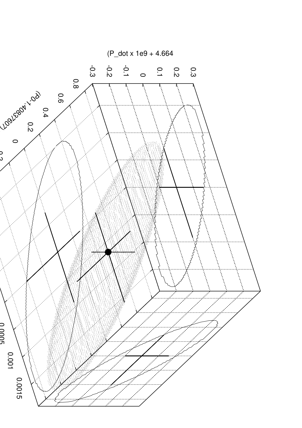
three-dimensional space ()
of errors. The region of admissible values and its projections
onto the corresponding planes of parameters are
shown in Fig. 6. For comparison, the line segments
indicate the errors calculated by assuming the parameters
to be independent. It follows from the figure that
the parameters have a significant correlation between
themselves and that the above errors were greatly
underestimated. Given all of the aforesaid, the final
solution for orbital motion appears as follows:
MJD
days
.
The latter value can be transformed to a more customary
and convenient form for comparison with the results
of previous measurements,
yr-1.
Comparison with the results of previous measurements
yr-1
(Levine et al. 2000) shows that the decay rate in the orbital period
in LMC X-4 is actually higher than has been thought previously.

Figure 7 shows the dependence of the orbital phase deviation from zero value (by definition, phase ‘‘0’’ correspond to the mid-eclipse) calculated from Eq.(1) with the orbital motion parameters obtained above (filled circles). To improve the visual perception of the figure, the data were grouped in time with a 30-day step. The dashed lines bound the error region within which all of the measurement results lie. For comparison, the triangles in the same figure indicate the orbital phase deviations obtained by using the orbital ephemerides of LMC X-4 from Levine et al. (2000). It can be seen that our model describes the orbital motion in LMC X-4 considerably better, but it was constructed fromthe data spanning amuch longer time interval. Such a significant increase of the observational data set is associated mainly with the series of deep observations of the Large Magellanic Cloud performed by the INTEGRAL observatory in 2003-2013 (Grebenev et al. 2013). Interestingly, the decay rate in the orbital period yr-1 obtained by Falanga et al. (2015), who used only the data from the first series of INTEGRAL observations of LMC X-4 in 2003-2004 in addition to the historical data, turns out to be similar to the results from Levine et al. (2000). The latter may suggest a change in the decay rate in the orbital period in the binary in the last decade, although the significance of these differences is low (about ).
Applying the solution obtained for the orbital motion in LMC X-4, we constructed an averaged profile of the dependence of the flux registered from the source on orbital phase from the data of four instruments operating in different X-ray bands (Fig. 8). To increase the statistical significance of the signal, we used only the data obtained near the maxima of the 30-day cycle . The averaged profiles constructed in this way in different energy bands are similar to one another in shape, as we have pointed out for the profiles of single eclipses.
Discussion
We presented the results of a comprehensive study of the long-term variability of the X-ray flux from the high-mass X-ray binary LMC X-4 based on the data of several space observatories over the last 25 years.

We obtained the mean precession period days, which may be considered as the equilibrium one over the time interval under consideration. Note significant variations of the period measured in each specific cycle near this value, causing the measured phase of the 30-day period to ‘‘walk’’ with respect to the phase predicted by the model with a constant period. The shape of the ‘‘walk’’ is very similar to the shape of the deviation of some quantity from its initial value in a ‘‘Brownian’’ process. Indeed, if we represent the expression to calculate the times of some phase in successive cycles as , where i is the cycle number and is the period of the jth cycle, and if assume that [] obey a normal distribution, then [] will have the frequency characteristic of ‘‘red noise’’ (corresponding to Brownian motion), which, by definition, is a ‘‘white noise’’ integral. Unfortunately, because of the insufficient quantity and quality of observational data, we cannot test this hypothesis by constructing the power spectrumof the time series. Nevertheless, if the suggested hypothesis is valid, then it is necessary to determine the processes responsible for the changes in the precession period. Two processes that explain the existence of the 30-day modulation are usually considered: tilted accretion disk precession or radiation-induced accretion disk warping. Neither of the two scenarios forbids the period variability, although they do not give a clear answer to the question of why and how this can occur.
Using long-term observations, we refined the orbital period in the binary system and its decay rate. In particular, this decay rate in the orbital period yr-1 turned out to be 20% higher than the values obtained previously (Levine et al. 2000; Falanga et al. 2015). The latter can be connected with a change in the decay rate in the orbital period in the last decade.
In general, investigating the orbital period changes can give valuable information about the evolution of close binaries and the mechanisms responsible for this process. For LMC X-4, the current orbital period has been measured many times: from the SAS-3 (Kelley et al. 1983), EXOSAT (Dennerl 1991), Ginga, RXTE (Levine et al. 1991, 2000), ROSAT (Levine 1996), and INTEGRAL (the first series of observations in 2003-2004; Falanga et al. 2015) data. Levine et al. (1991) were the first to point to a decrease in the orbital period in the binary and to obtain an upper limit on its derivative. Subsequently, using additional data, Safi-Harb et al. (1996) and Levine (2000) confirmed these conclusions. LMC X-4 is one of the five high-mass X-ray binaries (HMXBs) for which significant decreases in the orbital periods have been detected: LMC X-4, Cen X-3, 4U 1700-377, SMC X-1, and OAO 1657-415 (see the review of Falanga et al. 2015 and references therein). Various models were proposed to explain the observed changes in the orbital period (Kelley et al. 1983; van der Klis 1983, 1984; Levine et al. 1993, 2000; Rubin et al. 1996; Safi-Harb et al. 1996; Jenke et al. 2011). They are all based to some extent on two mechanisms that can lead to a decrease in the orbital period in the binary: tidal interactions and mass transfer due to a fast stellar wind, which characterizes most of the companion stars in HMXBs, or evolution of the companion star itself, in particular, its expansion and an increase in the moment of inertia, causing the star to spin down. The tidal angular momenta will then transfer this change to the orbital angular momentum to synchronize the binary, causing the orbital period to decrease (see, e.g., Levine et al. 1993, and references therein).
Our calculations show that both tidal interactions and mass transfer can play an important role for such a close binary as LMC X-4. The latter, in turn, must lead to a change in the accretion rate onto the neutron star and, as a consequence, to a change in its luminosity. This must be particularly noticeable in the last decade, when an increase in the rate of decrease in the orbital period is observed. Based on INTEGRAL data, we attempted to detect possible trends in the X-ray flux from LMC X-4, while the X-ray flux in such binaries must correlate with the mass transfer rate. For this purpose, we used only out-of-eclipse data near the precessional modulation maxima. From these results we concluded that, within the measurement error limits, the flux may be considered constant. Taking this into account, the model predicting a change in the orbital period due to the evolution of the normal star may be more plausible for the binary under consideration (recall that an O8 III giant is the companion star in it). To confirm or refute this hypothesis, it is necessary to perform optical monitoring observations and to compare them with the archival data, while its confirmation can become the first direct argument for the model of a change in the orbital period in the binary due to an evolving and expanding normal star.
ACKNOWLEDGMENTS
This work was financially supported by the Russian Foundation for Basic Research (project no. 13-02-12094 and grant President of Russian Federation NSh 6137.2014.2). We are grateful to E.M. Churazov, who developed the IBIS/INTEGRAL data analysis methods and provided the software. We thank the International Space Science Institute (Bern, Switzerland) for organizing a meeting on the theme of the publication.
References
1. H. V. Bradt, R. E. Rothschild, and J. H. Swank, Astrophys. J. Suppl. Ser. 97, 355 (1993).
2. C. Chevalier and S. A. Ilovaisky, Astron. Astrophys. 59, L9 (1977).
3. E. Churazov, R. Sunyaev, J. Isern, J. Knodlseder, P. Jean, F. Lebrun, N. Chugai, S. Grebenev, et al., Nature 512, 406 (2014).
4. W. I. Clarkson, P. A. Charles,M. J. Coe, and S. Laycock, Mon. Not. R. Astron. Soc. 343, 1213 (2003).
5. K. Dennerl, PhD Thesis (Max Planck Inst. Extraterrestr. Phys., Univ.Munchen, 1991).
6. A. Epstein, J. Delvaille, H. Helmken, S. Murray, H. W. Schnopper, R. Doxsey, and F. Primini, Astrophys. J. 216, 103 (1977).
7. M. Falanga, E. Bozzo, A. Lutovinov, J. M. Bonnet- Bidaud, Y. Fetisova, and J. Puls, Astron. Astrophys. 577, 16 (2015).
8. N. Gehrels, E. Chipman, and D. A. Kniffen, Astrophys. J. Suppl. Ser. 97, 5 (1993).
9. N. Gehrels, G. Chincarini, P. Giommi, K. D. Mason, J. A. Nousek, A. A. Wells, N. E. White, S. D. Barthelmy, et al., Astrophys. J. 611, 1005 (2004).
10. R. Giacconi, S. Murray, H. Gursky, E. Kellogg, E. Schreier, and H. Tananbaum, Astrophys. J. 178, 281 (1972).
11. S. Grebenev, A. Lutovinov, S. Tsygankov, and I. Mereminsky, Mon. Not. R. Astron. Soc. 428, 50 (2013).
12. J. B. Hutchings, D. Crampton, and A. P. Cowley, Astrophys. J., Part 1, 225, 548 (1978).
13. S. A. Ilovaisky, C. Chevalier, C. Motch, M. Pakull, J. van Paradijs, and J. Lub, Astron. Astrophys. 140, 251 (1984).
14. K. Jahoda, C. B. Markwardt, Y. Radeva, A. H. Rots, M. J. Stark, J. H. Swank, T. E. Strohmayer, and W. Zhang, Astrophys. J. Suppl. Ser. 163, 401 (2006).
15. R. I. Kelley, J.G. Jernigan, A. Levine, L. D. Petro, and S. Rappaport, Astrophys. J. 264, 568 (1983).
16. M.M. Kotze and P. A. Charles, Mon. Not. R. Astron. Soc. 420, 1575 (2012).
17. H. A. Krimm, S. T. Holland, R. H. D. Corbet, A. B. Pearlman, P. Romano, J. A. Kennea, J. S. Bloom, S. D. Barthelmy, et al., Astrophys. J. Suppl. Ser. 209, 14 (2013).
18. R. Krivonos, M. Revnivtsev, S. Tsygankov, S. Grebenev, E. Churazov, and R. Sunyaev, Astron. Astrophys. 519, A107 (2010).
19. F. L. Lang, A. M. Levine, M. Bautz, S. Hauskins, S. Howe, F. A. Primini, W. H. G. Lewin, W. A. Baity, et al., Astrophys. J. 246, L21 (1981).
20. A. Levine, S. Rappaport, A. Putney, R. Corbet, and F. Nagase, Astrophys. J. 381, 101 (1991).
21. A. M. Levine, H. Bradt, W. Cui, J. G. Jernigan, E. H. Morgan, R. Remillard, R. E. Shirey, and D. A. Smith, Astrophys. J. Lett. 469, L33 (1996).
22. A. M. Levine, S. A. Rappaport, and G. Zojchenski, Astrophys. J. 541, 194 (2000).
23. F. Li, S. Rappaport, and A. Epstein, Nature 271, 37 (1978).
24. M. Matsuoka, K. Kawasaki, S. Ueno, H. Tomida, M. Kohama, M. Suzuki, Y. Adachi, M. Ishikawa, et al., Publ. Astron. Soc. Jpn. 61, 999 (2009).
25. van derMeer, Ph.D. Thesis (Astron. Inst.Anton Pannekoek, Univ. Amsterdam, The Netherlands, 2006).
26. D. Moon and S. Eikenberry, Astrophys. J. 549, L225 (2001).
27. W. Pietsch, W. Voges, M. Pakull, and R. Staubert, Space Sci. Rev. 40, 371 (1985).
28. S. Safi-Harb, H. Ogelman, and K. Dennerl, Astrophys. J. 456, L37 (1996).
29. N. Sanduleak and A. G. D. Philip, IAU Circ., No. 3023 (1977).
30. W. M. Smart, Celestial Mechanics (Green and Co, Longmans, 1953).
31. L. Struder, U. Briel, K. Dennerl, R. Hartmann, E. Kendziorra, N.Meidinger, E. Pfeffermann, C. Reppin, et al., Astron. Astrophys. 365, L18 (2001).
32. S. S. Tsygankov and A. A. Lutovinov, Astron. Lett. 31, 380 (2005).
33. P. Ubertini, F. Lebrun, G. Di Cocco, A. Bazzano, A. J. Bird, K. Broenstad, A. Goldwurm, G. La Rosa, et al., Astron. Astrophys. 411, L131 (2003).
34. N. E.White, Nature 271, 38 (1978).
35. C. Winkler, T. Courvoisier, G. Di Cocco, N. Gehrels, A. Gimenez, S. Grebenev, W. Hermsen, J. M. Mas- Hesse, et al., Astron. Astrophys. 411, L1 (2003).
36. J. W. Woo, G. W. Clark, A. M. Levine, R. H. Corbet, and F. Nagase, Astrophys. J. 467, 811 (1996).
Table 3. Mid-eclipse times for LMC X-4 from the data of various instruments
| Mid-eclipse | Instrument | Mid-eclipse | Instrument |
| (MJD) | (MJD) | ||
| SAS-3 | INTEGRAL | ||
| optics | INTEGRAL | ||
| EXOSAT | INTEGRAL | ||
| EXOSAT | INTEGRAL | ||
| EXOSAT | INTEGRAL | ||
| EXOSAT | INTEGRAL | ||
| GINGA | INTEGRAL | ||
| GINGA | INTEGRAL | ||
| ROSAT | INTEGRAL | ||
| RXTE/PCA | INTEGRAL | ||
| RXTE/PCA | INTEGRAL | ||
| RXTE/PCA | INTEGRAL | ||
| RXTE/PCA | INTEGRAL | ||
| INTEGRAL | INTEGRAL | ||
| INTEGRAL | INTEGRAL | ||
| XMM-Newton | INTEGRAL | ||
| INTEGRAL | INTEGRAL | ||
| INTEGRAL | INTEGRAL | ||
| XMM-Newton | INTEGRAL | ||
| INTEGRAL | INTEGRAL | ||
| INTEGRAL | INTEGRAL | ||
| INTEGRAL | INTEGRAL | ||
| INTEGRAL | INTEGRAL | ||
| INTEGRAL | INTEGRAL | ||
| INTEGRAL | INTEGRAL | ||
| INTEGRAL | INTEGRAL | ||
| a ‘‘based on the Doppler effect’’ (see the text) (Kelley et al. 1983) | |||
| b from the optical 19762̆0131983 observations (Ilovaisky et al. 1984) | |||
| c Dennerl (1991) | |||
| d Pietsch et al. (1985) | |||
| e ’’based on the Doppler effect’’ (Woo et al. 1996) | |||
| f ’’based on the Doppler effect’’ (Levine et al. 1991) | |||
| g eclipse was observed partially | |||
| h a conservative estimate of the error from above (see the text) | |||
| i see also Falanga et al. (2015) | |||
| j light curves with eclipses are also given in van derMeer (2006) | |||