CERN-PH-TH-2015-219
Topological Susceptibility from Slabs
Wolfgang Bietenholz, Philippe de Forcrand and Urs Gerber
Instituto de Ciencias Nucleares
Universidad Nacional Autónoma de México
A.P. 70-543, C.P. 04510 Distrito Federal, Mexico
Institute for Theoretical Physics, ETH Zürich
CH-8093 Zürich, Switzerland
CERN, Physics Department, TH Unit
CH-1211 Geneva 23, Switzerland
Instituto de Física y Matemáticas
Universidad Michoacana de San Nicolás de Hidalgo
Edificio C-3, Apdo. Postal 2-82
C.P. 58040, Morelia, Michoacán, Mexico
In quantum field theories with topological sectors, a non-perturbative quantity of interest is the topological susceptibility . In principle it seems straightforward to measure by means of Monte Carlo simulations. However, for local update algorithms and fine lattice spacings, this tends to be difficult, since the Monte Carlo history rarely changes the topological sector. Here we test a method to measure even if data from only one sector are available. It is based on the topological charges in sub-volumes, which we denote as slabs. Assuming a Gaussian distribution of these charges, this method enables the evaluation of , as we demonstrate with numerical results for non-linear -models.
1 The topological susceptibility
There are a number of models in quantum field theory, which have the property that the configurations occur in distinct topological sectors; each sector is characterised by a topological charge . This refers either to infinite volume and configurations with finite actions, or to finite volume with periodic boundary conditions. Here we consider the latter setting, with some volume in Euclidean space.
The models with this property include in particular 4d Yang-Mills theories for all . Fermions may be present as well, so this class of models encompasses QCD. In that case, the quenched value of the topological susceptibility has a prominent application in the explanation of the heavy mass of the pseudo-scalar -meson [1].
The measurement of is a non-perturbative issue, hence lattice simulations are the appropriate method. If the Monte Carlo history changes frequently, this measurement is straightforward. However, for most of the popular algorithms, including local update algorithms, as well as the Hybrid Monte Carlo algorithm (which is standard in QCD with dynamical quarks), the auto-correlation time with respect to tends to be very long, in particular on fine lattices.11 1 In general, the topological sectors are well-defined only in the continuum limit (there are exceptions for lattice actions with a constraint that only admits very smooth configurations [2, 3, 4]). So in general transitions are only enabled by lattice artifacts, and by discrete jumps of the algorithm. This problem is getting even worse in the presence of chiral fermions.
Recently, several indirect methods to measure nevertheless have been suggested and tested [5, 6]. Here we address a different approach for this purpose, which was first sketched in Ref. [7], but which has not been explored ever since (though a similar approach was studied last year [8]). It is described in Section 2. Sections 3 and 4 give results for the 1d and the 2d model, respectively. Our conclusions are discussed in Section 5, and an appendix is devoted to analytical considerations about artifacts in .
2 Evaluating from slabs
We assume parity symmetry to hold, which implies . We further assume the topological charges to obey a Gaussian probability distribution,22 2 The assumption of a Gaussian distribution of the topological charges appears natural in light of instanton gas models. In case of the quantum rotor in infinite volume, it can be demonstrated analytically [9]. Simulations confirm that it also holds — at least to a good approximation — in the 2d model [6] (cf. Section 4), and in QCD [10].
| (2.1) |
The idea of the method that we are going to explore, is to divide the periodic volume into sub-volumes, which we denote as slabs, and to extract from the fluctuations of the topological charge within these slabs. This has the potential of providing the result even based on configurations of a single topological sector (with respect to the entire volume ).
We consider just two slabs, of sizes and , where .33 3 The extension of this method to a larger number of slabs is straightforward, but hardly promising, since the slab volumes should not be too small. At fixed charge , we denote the topological charge contribution in the first slab as ; it is obtained by integrating the topological charge density over the slab volume. In general it is not an integer, because not all slab boundaries are periodic. Thus we obtain the probability for the charge contributions and in the two slabs,
| (2.2) | |||||
where we defined .
Eq. (2.2) implies , and therefore
| (2.3) |
Thus, if we measure at a set of values in a fixed sector with topological charge , we can fit the results for to the parabola , which is predicted by eqs. (2.2) and (2.3).
The simplest case is the topologically trivial sector, , where is given by a parabola, which takes its maximum at , with a value of . In the topologically charged sectors, still has the same shape, whereas is a parabola that connects with . In any sector, the measured data for can be fitted to the expected parabola. The susceptibility is the only fitting parameter, which is evaluated in this manner.
3 Results for the quantum rotor
We first consider a quantum mechanical scalar particle moving freely on a unit circle. We deal with periodic boundary conditions in Euclidean time. Then there is an integer winding number for each trajectory, which characterises the topological sectors of this model. It is also denoted as the 1d model, or 1d XY model, and it is related to 2d gauge theory [11].
Now we assume Euclidean time to be uniformly discretised, and on each site there is an angular variable (with ). We apply the geometric definition of the topological charge [12],
| (3.1) |
where we define the modulo function such that is the shortest arc length connecting nearest neighbour angular variables.
In our numerical studies we simulated three lattice actions: the standard action, the Manton action [13] and the constraint action [3],44 4 The constraint action is a special case of a topological lattice action [3, 4, 14], which is characterised by the property that the action remains invariant under most small variations of a configuration.
The continuum limit is attained at or .
Our simulations were all performed with a cluster algorithm [15]. Due to its non-local update steps, the Markov chain changes the topological sector frequently, which enables a precise direct measurement of the topological susceptibility. This result is then confronted with the value determined by the slab method, described in Section 2.
We begin with an illustration of measured data for the probability product in eq. (2.2), as a function of the relative slab width (here the “slab” is actually just an interval in Euclidean time).
As a first example, Figure 1 shows data for , as a function of . These values were measured with the standard action at size and , which implies a correlation length of . We see that the curves obtained in the sectors , and do follow the expected parabolas, which interpolate and , as predicted in Section 2.
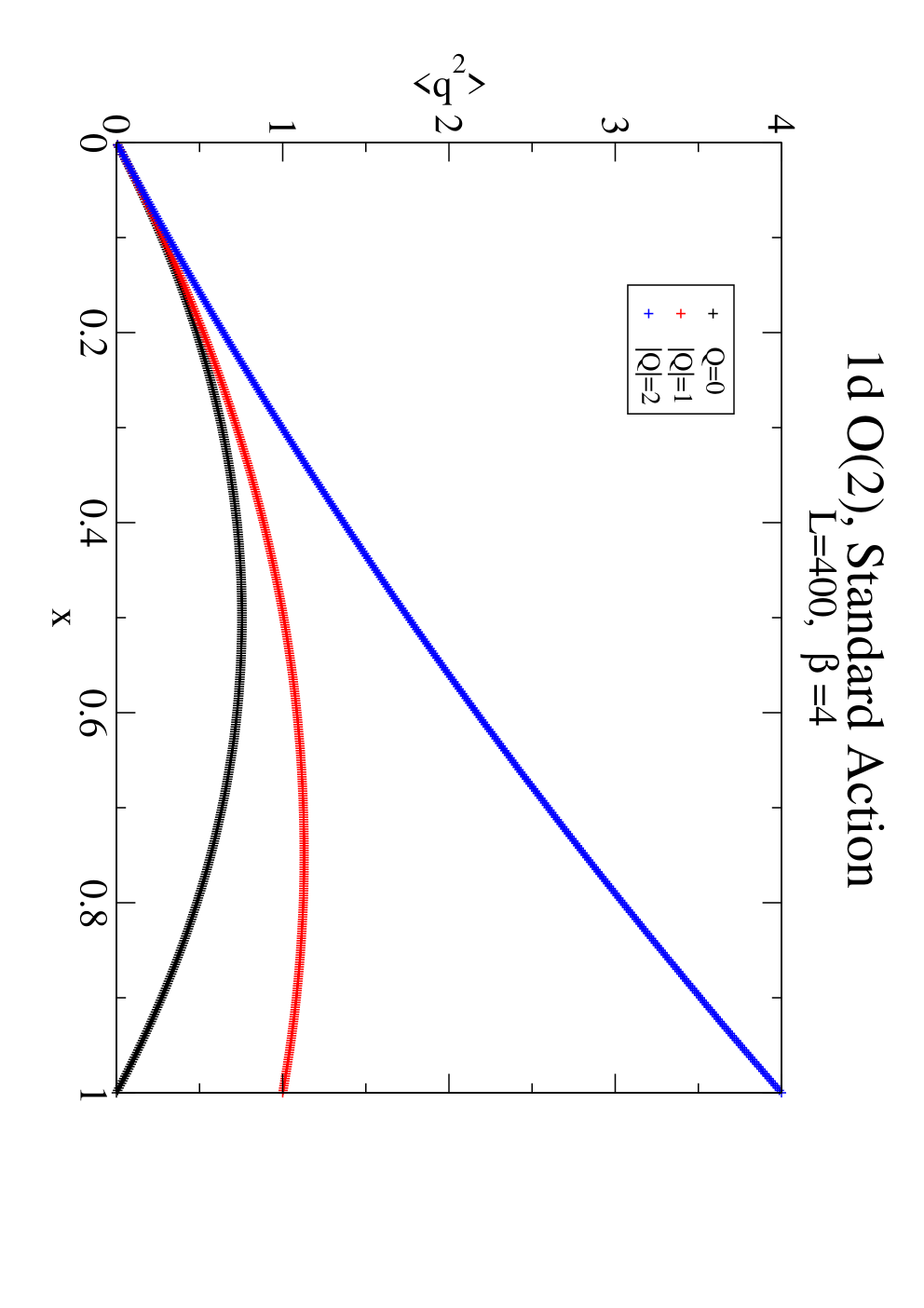
Next we give results obtained with the constraint action,
now at and ,
where the correlation length is short, .
Figure 2 shows again the numerical data for
as a function of ,
in the sectors , and .
For comparison, we also include the parabola for the
function , which is predicted for
. Here we insert the directly measured
value of . We see in all cases accurate agreement
between this prediction and the numerical data.


Let us proceed to a quantitative discussion.
We start again with the standard action, where we consider
and . In a variety of sizes we
applied the slab method, and evaluated by a
fit of the data for to the predicted
parabola. The results are given in Table 1.
Figure 3 shows the corresponding convergence
of the scaling term , where is the
correlation length.55
5
Here and in Figures
2 and 5 we insert
the analytic values for , which are also given in Tables
1, 2 and
3. They were calculated with the
formulae given in Refs. [9] and [3] as functions
of and , see also Tables 1,
2 and 3.
This refers to ,
but since holds in all cases, this is not problematic.
They are consistently close to the analytical value at infinite
(the corresponding formula is given in Ref. [9]).
That value is in all cases compatible with the directly measured
, which is also included in Table 1.
For increasing the agreement with the slab method results
improves further.


| direct | ||||
|---|---|---|---|---|
| 100 | 0.019369(6) | 0.019280(7) | 0.019324(11) | 0.019480(29) |
| 200 | 0.019372(8) | 0.019346(14) | 0.019314(10) | 0.019326(19) |
| 400 | 0.019365(10) | 0.019348(16) | 0.019337(11) | 0.019333(19) |
| 150 | 0.007554(3) | 0.007534(4) | 0.007550(6) | 0.007587(2) |
| 200 | 0.007557(3) | 0.007541(3) | 0.007547(4) | 0.007581(8) |
| 250 | 0.007549(3) | 0.007542(3) | 0.007550(4) | 0.007585(8) |
| 300 | 0.007560(4) | 0.007545(3) | 0.007545(5) | 0.007554(5) |
| 350 | 0.007554(5) | 0.007545(4) | 0.007557(2) | 0.007553(5) |
| 400 | 0.007549(5) | 0.007552(4) | 0.007551(3) | 0.007564(5) |
Next we give analogous results for the Manton action,
Figure 4 and Table 2,
and for the constraint action, Figure 5
and Table 3. Qualitatively the same
features are confirmed. Quantitatively we see that the
Manton action — which is classically perfect [9] —
performs very well regarding the convergence
towards the value at . For all actions,
the convergence is best for , while
is affected by somewhat stronger finite size effects.


| direct | ||||
|---|---|---|---|---|
| 100 | 0.012658(7) | 0.012666(5) | 0.012666(9) | 0.012631(22) |
| 200 | 0.012661(4) | 0.012656(7) | 0.012661(6) | 0.012659(14) |
| 400 | 0.012653(4) | 0.012672(7) | 0.012658(7) | 0.012666(11) |
| 150 | 0.006330(4) | 0.006331(3) | 0.006332(4) | 0.006316(2) |
| 200 | 0.006333(3) | 0.006330(2) | 0.006328(4) | 0.006339(9) |
| 250 | 0.006335(3) | 0.006336(3) | 0.006333(3) | 0.006339(8) |
| 300 | 0.006332(3) | 0.006333(4) | 0.006333(2) | 0.006316(9) |
| 350 | 0.006334(4) | 0.006329(3) | 0.006335(4) | 0.006342(7) |
| 400 | 0.006329(3) | 0.006330(3) | 0.006334(3) | 0.006323(5) |


| direct | ||||
| 100 | 0.037036(13) | 0.037281(16) | 0.037183(14) | 0.036990(35) |
| 200 | 0.037008(15) | 0.037163(20) | 0.037121(18) | 0.037079(29) |
| 400 | 0.037042(19) | 0.037091(33) | 0.037109(23) | 0.037056(26) |
| 100 | 0.018987(8) | 0.019113(8) | 0.019058(10) | 0.018864(28) |
| 200 | 0.019011(9) | 0.019050(9) | 0.019049(13) | 0.018983(17) |
| 400 | 0.018992(7) | 0.019038(13) | 0.019032(8) | 0.019019(12) |
| 100 | 0.008443(5) | 0.008491(3) | 0.008416(10) | 0.008208(36) |
| 200 | 0.008445(4) | 0.008475(5) | 0.008452(7) | 0.008397(16) |
| 400 | 0.008439(5) | 0.008460(5) | 0.008455(6) | 0.008445(15) |
We also verified that and the kurtosis term (which is related to the Binder cumulant),
| (3.5) |
are both compatible with in all cases (within at most ).66 6 For these parameters and huge statistics of measurements, the error in can be reduced to , and one observes significant deviations from zero [6]. However, these tiny values have no influence on the interpretation of the results presented here. The former follows from parity symmetry, and a Gaussian -distribution implies . The vanishing of these two quantities is an assumption of the slab method. For the kurtosis this condition is not trivial; it will be considered in detail in the next section.
Another source of systematic errors are artifacts in due to the finite size and finite lattice spacing. These artifacts are discussed in Appendix A.
4 Results for the 2d Heisenberg model
We proceed to the 2d model, where we consider square lattices with classical spins on the sites . In order to define the topological charge, we cut each plaquette into two triangles (with an alternating orientation between adjacent plaquettes). For a triangle with sites we identify the (minimal) solid angle spanned by , , , including a sign factor for its orientation (a fully explicit description is given in Ref. [3]).
The sum of the two oriented solid angles within a plaquette,
divided by , defines the
topological charge density . The total charge of a
spin configuration amounts to
. It counts how many
times the sum of these solid angles covers the sphere
with a definite orientation.
In analogy to Section 3, we consider three lattice actions, including an obvious generalisation of the Manton action, which was simulated with a new variant of the Wolff cluster algorithm,
Regarding the application of the slab method with these lattice actions, Figure 6 shows results obtained in the lattice volumes and .


We also consider further volumes, including rectangular shapes. In fact, it is not obvious if the slab method results should be compared to in the entire (periodic) volume , or to in a (non-periodic) slab of size . Hence we have measured the latter as well, for comparison. The detailed results, along with the corresponding correlation length, are given in Tables 4, 5 and 6.77 7 In this model, the apparent scaling quantity diverges logarithmically in the continuum limit (see e.g. Ref. [3]), so here we refer directly to . However, for volumes, which are large enough for the slab method to work quite well, it turns out that and are too close to each other to be distinguished in light of the slab method results.
| 1 | 0.01715(2) | 0.01718(2) | 0.01714(2) | 0.01723(2) | 0.01705(2) | |
| 0.01716(3) | 0.01717(2) | 0.01718(2) | 0.01717(2) | 0.01726(2) | ||
| 1.5 | 0.002319(3) | 0.002354(2) | 0.002305(5) | 0.002322(5) | 0.002361(5) | |
| 0.002332(5) | 0.002356(3) | 0.002327(4) | 0.002327(4) | 0.002358(4) | ||
| 0.002332(4) | 0.002344(3) | 0.002304(3) | 0.002321(2) | 0.002324(3) | ||
| 0.002341(3) | 0.002359(3) | 0.002333(3) | 0.002337(3) | 0.002352(3) | ||
| 0.002327(3) | 0.002347(3) | 0.002390(10) | 0.002381(9) | 0.002371(9) | ||
| 0.002334(4) | 0.002342(3) | 0.002353(1) | 0.002351(1) | 0.002366(1) |
| 0.5 | 0.02329(4) | 0.02333(3) | 0.02330(3) | 0.02339(2) | 0.02330(2) | |
| 0.02335(2) | 0.02335(3) | 0.02330(2) | 0.02343(2) | 0.02330(2) | ||
| 0.75 | 0.00954(2) | 0.00956(1) | 0.00953(2) | 0.00952(2) | 0.00952(2) | |
| 0.00953(2) | 0.00957(1) | 0.00962(2) | 0.00955(1) | 0.00957(2) |
| 0.02157(5) | 0.02155(2) | 0.02145(2) | 0.02162(2) | 0.02149(2) | ||
| 0.02144(4) | 0.02151(3) | 0.02144(2) | 0.02149(2) | 0.02156(2) | ||
| 2 | 0.01545(2) | 0.01547(2) | 0.01549(2) | 0.01546(1) | 0.01543(2) | |
| 0.01549(3) | 0.01547(2) | 0.01538(2) | 0.01541(1) | 0.01543(1) | ||
| 0.002445(6) | 0.002663(4) | 0.002168(65) | 0.003806(14) | 0.005211(27) | ||
| 0.002795(4) | 0.002873(3) | 0.002816(17) | 0.002888(16) | 0.003146(15) | ||
| 0.002797(4) | 0.002835(4) | 0.002859(6) | 0.002853(7) | 0.002850(7) | ||
| 0.002795(4) | 0.002816(3) | 0.002826(3) | 0.002812(3) | 0.002810(3) | ||
| 0.002792(5) | 0.002818(3) | 0.002831(4) | 0.002835(4) | 0.002843(4) | ||
| 0.002783(6) | 0.002805(3) | 0.002837(3) | 0.002828(3) | 0.002819(3) |
The assumption of a Gaussian distribution of the topological charges is essential for the viability of this method. Figure 7 shows that the kurtosis (3.5) — as a measure for the deviation from a Gaussian — decreases rapidly as we approach the continuum limit; for the Manton action we see an exponential decrease of as increases. Thus a non-zero value of appears as a lattice artifact, and not as a finite size effect; this observation agrees qualitatively with a discussion in Ref. [6]. This artifact is much less suppressed for the standard action and the constraint action. Regarding the application of the slab method with these lattice actions, Figure 6 shows results obtained in the lattice volume and . The systematic errors of the slab method appear as tiny deviations of extracted from and (three rightmost points in each set of four) from the directly measured value (leftmost point).


5 Conclusions
We have tested an unconventional method for the numerical measurement of the topological susceptibility , based on the division of the volume into slabs. This method is applicable even if configurations in only one topological sector are available.
Our study shows that — under suitable conditions — this method works very well. Its statistical accuracy is comparable to the precision in the absence of “topological slowing down”, i.e. the slab method is not affected by the freezing of the topological sectors.
In particular, we obtained in the 2d model results for , which are correct on the percent level, and in the 1d far beyond. This precision was revealed by large statistics of measurements, which would not be accessible in higher dimensional models like QCD; in this sense, the accuracy of the slab results are fully satisfactory.
The slab method is most successful at small topological charges, , whereas its application in the sector is more tedious, since the finite size effects are worse. However, even at the finite size effects are highly persistent. In fact, other methods and formulae show that these effects are only suppressed by a power series in for topologically fixed measurements [5, 6].
As an illustrative example of possible systematic effects, we refer to the results at in Table 6: even the smallest volume, , corresponds to the ratio , where one would expect usual (i.e. exponentially suppressed) finite size effects to be mostly eliminated. The results for the slab method, however, are strongly distorted — they improve significantly at (and for it even takes ).
This illustrates the general feature: at fixed or , i.e. at approximately constant , the slab results converge for increasing volume. In order to assure that they do converge to the (vicinity of the) correct value, we further have to require the topological charges to be (approximatively) Gauss-distributed (that also ensures a good fit to formula 2.2). Therefore we also studied the kurtosis, which may deviate from zero (indicating a deviation from a Gaussian) as a lattice artifact. It is suppressed when increases (in lattice units), with a rate that depends on the lattice action; for the Manton action we observed a particularly fast, exponential suppression.
Hence should be sufficiently large to control that requirement, and the volume should be large enough to obtain ; then the slab method can be expected to provide the correct value on the percent level.
Acknowledgements
We thank Irais Bautista and Christoph P. Hofmann for inspiring discussions. This work was supported in part
by the Mexican Consejo Nacional de Ciencia y Tecnología
(CONACYT) through projects CB-2010/155905 and
CB-2013/222812, and by DGAPA-UNAM, grant IN107915.
Appendix A Artifacts in the topological susceptibility
An essential point for the quality of the results obtained by the slab method is the precision of as measured in the sub-volumes. In this appendix we discuss the artifacts that occur: Sub-Appendix A.1 deals with the finite size effects, which depend on the ratio , and which even occur in the continuum formulation. Sub-Appendix A.2 considers the lattice artifacts, as a function of (where is the lattice spacing, and is now the dimensional size). Both considerations are performed in the analytically tractable case of the quantum rotor; Sub-Appendix A.2 captures the standard and the Manton action. For simplicity we deal with periodic boundary conditions throughout, although they are partly open in the sub-volumes, so we assume implicitly that is large enough for this distinction to be negligible.
A.1 Finite size effects
While the slab method is plagued by particularly persistent finite size effects, the true value tends to converge exponentially as the volume is enlarged. Here we discuss this convergence for the case of the 1d model.
In the continuum formulation, with the action , the topological susceptibility takes the form [9]
| (A.1) |
It can be written in terms of a Jacobi -function,
| (A.2) |
By applying the Jacobi identity,
| (A.3) |
we obtain
| (A.4) |
Inserting approximation (A.4) into formula (A.2), we arrive at
| (A.5) |
With the correlation length [9], this corresponds to the ratio
| (A.6) |
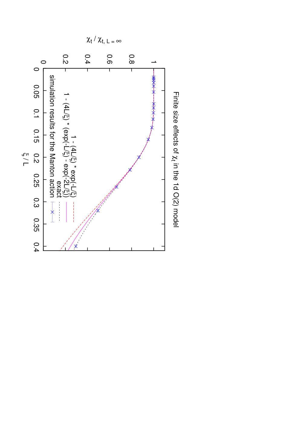
Thus we see explicitly the exponentially suppressed finite size corrections. Figure 8 illustrates this formula, and compares it to the exact result (numerical summation of the series in eq. (A.1)), which agrees with simulation data for the Manton action at (where lattice artifacts are practically erased).
A.2 Lattice artifacts
We begin with general properties of a field theory in a periodic Euclidean volume , where the configurations of the field are divided into topological sectors. In presence of a vacuum angle (and with ), the partition function and the topological susceptibility can be written as88 8 Occasionally we omit the argument in the partition function and (below) in the energy eigenvalues.
| (A.7) |
In the Hamilton formulation, the partition function reads
where is the inverse temperature, and we assume a discrete energy spectrum. Inserting eq. (A.7) leads to
| (A.8) |
Now we focus on , and replace and both by (the periodicity range in Euclidean time). More specifically, we consider again the quantum rotor, where also represents the moment of inertia. We deal with a lattice of spacing , and periodicity over sites, . A consideration of the transfer matrix yields [9]
where , and
In either case, is even, such that , in accordance with , and some algebra leads to
| (A.9) | |||||
To proceed, we now have to specify . We start with the Manton action, and substitute ,
| (A.10) |
If we write and in exponential form, and complete the squares in the exponents,
| (A.11) |
we see several types of lattice artifacts, such as the
extra term in the exponent, and the
incomplete Gauss integrals; they are exponentially
suppressed in . The substitution of the integration variable
corresponds to a shift of the integration contour;
for the incomplete Gauss integral this
is another artifact, which is exponentially suppressed.
In summary, there are no power lattice artifacts for the Manton action.
For the standard action the corresponding formulae read
| (A.12) | |||||
Regarding the search for power lattice artifacts, we start from the Manton action and add the two leading modifications of the standard action, . This modifies the expressions for , and in eq. (A.10) by a factor
under the integrals, and after some calculus we obtain
| (A.13) |
Hence for the standard action is affected by corrections linear in .
This may appear surprising for a bosonic theory, but one has to keep in mind that is not a scaling quantity. The actual scaling artifacts refer to the product . In the thermodynamic limit they are expressed in powers of [3],
For the standard action, the linear artifacts cancel in this scaling
quantity, while the Manton action is classically perfect; its scaling artifacts are
exponentially suppressed. As an exotic feature, the constraint action
does have linear artifacts, due to the absence of a derivative term
in the action.
We summarise that the finite size effects are exponentially suppressed in , whereas the type of lattice artifacts depend on the lattice action.
References
- [1] E. Witten, Nucl. Phys. B 156 (1979) 269. G. Veneziano, Nucl. Phys. B 159 (1979) 213.
- [2] M. Lüscher, Nucl. Phys. B 549 (1999) 295 [hep-lat/9811032].
- [3] W. Bietenholz, U. Gerber, M. Pepe and U.-J. Wiese, JHEP 12 (2010) 020 [arXiv:1009.2146 [hep-lat]].
- [4] O. Akerlund and P. de Forcrand JHEP 1506 (2015) 183 [arXiv:1505.02666 [hep-lat]].
- [5]
R. Brower, S. Chandrasekharan, J.W. Negele
and U.-J. Wiese, Phys. Lett. B 560 (2003) 64
[hep-lat/0302005].
S. Aoki, H. Fukaya, S. Hashimoto and T. Onogi, Phys. Rev. D 76 (2007) 054508 [arXiv:0707.0396 [hep-lat]].
S. Aoki et al. (JLQCD and TWQCD Collaborations), Phys. Lett. B 665 (2008) 294 [arXiv:0710.1130 [hep-lat]].
W. Bietenholz, I. Hip, S. Shcheredin and J. Volkholz, Eur. Phys. J. C 72 (2012) 1938 [arXiv:1109.2649 [hep-lat]].
A. Dromard and M. Wagner, Phys. Rev. D 90 (2014) 074505 [arXiv:1404.0247 [hep-lat]].
H. Fukaya, S. Aoki, G. Cossu, S. Hashimoto, T. Kaneko and J. Noaki (JLQCD Collaboration), arXiv:1411.1473 [hep-lat]. - [6] I. Bautista, W. Bietenholz, A. Dromard, U. Gerber, C.P. Hofmann, H. Mejía-Díaz and M. Wagner, arXiv:1503.06853 [hep-lat].
- [7] P. de Forcrand, M. García Pérez, J.E. Hetrick, E. Laermann, J.F. Lagae and I.O. Stamatescu, Nucl. Phys. Proc. Suppl. 73 (1999) 578 [hep-lat/9810033].
- [8] R.C. Brower et al. (LSD Collaboration), Phys. Rev. D 90 (2014) 014503 [arXiv:1403.2761 [hep-lat]].
- [9] W. Bietenholz, R. Brower, S. Chandrasekharan and U.-J. Wiese, Phys. Lett. B 407 (1997) 283 [hep-lat/9704015].
- [10] S. Dürr, Z. Fodor, C. Hoelbling and T. Kurth, JHEP 0704 (2007) 055 [hep-lat/0612021].
- [11] R. Sinclair, Phys. Rev. D 45 (1992) 2098.
- [12] B. Berg and M. Lüscher, Nucl. Phys. B 190 (1981) 412.
- [13] N. Manton, Phys. Lett. B 96 (1980) 328.
- [14]
W. Bietenholz, M. Bögli, F. Niedermayer,
M. Pepe, F.G. Rejón-Barrera and U.J. Wiese,
JHEP 1303 (2013) 141 [arXiv:1212.0579 [hep-lat]].
W. Bietenholz, U. Gerber and F.G. Rejón-Barrera, J. Stat. Mech. (2013) P12009 [arXiv:1307.0485 [hep-lat]]. - [15] U. Wolff, Phys. Rev. Lett. 62 (1989) 361.