跳到论文正文
W Papers独立论文阅读器 arXiv:1509.06403 论文正文 计算阅读时间 · 0%
引用这篇论文根据当前论文元数据生成,正式投稿前建议核对。


License: arXiv.org perpetual non-exclusive license
arXiv:1509.06403v2 [stat.ME] 13 Oct 2015

Consistency bands for the mean excess function and application to graphical goodness of fit test for financial data

Abstract.

In this paper, we use the modern setting of functional empirical processes and recent techniques on uniform estimation for non parametric objects to derive consistency bands for the mean excess function in the i.i.d. case. We apply our results for modelling financial data, in particular Dow Jones data basis to see how good the Generalized hyperbolic distribution models fit monthly data.


Keyswords: ​Mean excess function, Vapnik-Chervonenkis classes, Entropy numbers, Bracketing numbers, Glivenko-Cantelli and Donsker classes, Functional empirical processes, Stochastic processes, Talagrand bounds, Generalized hyperbolic distributions.

Gane Samb Lo(1,2), Diadie Ba(2), Elhadji Deme(2) and Cheikh T. Seck(2,3).

(1)LSA, Université Pierre et Marie Curie, France.
(2)
LERSTAD, Université Gaston Berger, Sénégal.
(3)
Université de Bambey, Sénégal.

1. Introduction

Let XX be a random variable defined on a probability space (Ω,𝒜,ℙ),(\Omega,\mathcal{A},\mathbb{P}), and let FF be its distribution function with endpoint

xF=sup{x∈ℝ,F⁡(x)<1},x_{F}=\sup\{x\in\mathbb{R},F(x)<1\},

and let F¯=1−F\bar{F}=1-F its survival function.

Throughout the paper we suppose that 𝔼​|X|<∞\mathbb{E}|X|<\infty. The mean excess function e⁡(u)e(u) of XX is defined by (see, e.g., Kotz and Shanbhag [6], Hall and Wellner [5], Guess and Proschan [4])

(1.1) e⁡(u)=𝔼⁡(X−u/X>u)={1F¯​(u)​∫u∞F¯​(t)​dtifF¯​(u)>00wheneverF¯​(u)=0.e(u)=\mathbb{E}(X-u/X>u)=\left\{\begin{array}[]{l}\displaystyle\frac{1}{\bar{F}(u)}\int_{u}^{\infty}\bar{F}(t)dt\ \ \mbox{if}\ \ \bar{F}(u)>0\cr\cr\displaystyle 0\ \ \ \ \ \ \ \ \ \ \ \ \ \ \ \mbox{whenever}\ \ \ \bar{F}(u)=0.\cr\end{array}\right.

A natural way to estimate the mean excess function e⁡(u)e(u) is achieved by using the plug-in method, that is replacing the survival function in (1.1) by its empirical counterpart, as did Yang [3].

Now consider a sequence X1,X2,…X_{1},X_{2},... of independent copies of XX. The plug-in estimator of e⁡(u)e(u), for n≥1n\geq 1, is

(1.2) en​(u)=∑i=1n(Xi−u)𝕀[Xi>u]∑i=1n𝕀[Xi>u]=∑i=1nXi𝕀[Xi>u]∑i=1n𝕀[Xi>u]−u,{e}_{n}(u)=\frac{\sum_{i=1}^{n}(X_{i}-u)\mathbb{I}_{[X_{i}>u]}}{\sum_{i=1}^{n}\mathbb{I}_{[X_{i}>u]}}=\frac{\sum_{i=1}^{n}X_{i}\mathbb{I}_{[X_{i}>u]}}{\sum_{i=1}^{n}\mathbb{I}_{[X_{i}>u]}}-u,

where 𝕀[X>u]=1\mathbb{I}_{[X>u]}=1 if X>uX>u and 00 otherwise.

For notation convenience, we denote

ℙX​(fu)=∫fu​(x)​𝑑F​(x)=∫ux​𝑑F​(x)\mathbb{P}_{X}(f_{u})=\int f_{u}(x)dF(x)=\int_{u}xdF(x)

and

ℙX​(gu)=∫gu​(x)​𝑑F​(x)=∫ud​F​(x)=F¯​(u)\mathbb{P}_{X}(g_{u})=\int g_{u}(x)dF(x)=\int_{u}dF(x)=\bar{F}(u)

where fu(x)=x𝕀[x>u],gu(x)=𝕀[x>u],f_{u}(x)=x\mathbb{I}_{[x>u]},\ \ g_{u}(x)=\mathbb{I}_{[x>u]}, and ℙX\mathbb{P}_{X} is the probability law of XX.

We also denote by ℙn\mathbb{P}_{n} the empirical measure associated with the sample X1,⋯,XnX_{1},\cdots,X_{n}. We have

ℙn(fu)=1n∑i=1nXi𝕀[Xi>u]andℙn(gu)=1n∑i=1n𝕀[Xi>u].\mathbb{P}_{n}(f_{u})=\frac{1}{n}\sum_{i=1}^{n}X_{i}\mathbb{I}_{[X_{i}>u]}\ \ \text{and}\ \ \ \mathbb{P}_{n}(g_{u})=\frac{1}{n}\sum_{i=1}^{n}\mathbb{I}_{[X_{i}>u]}.

Formulae (1.1) and (1.2) lead to

e⁡(u)={ℙX​(fu)ℙX​(gu)−uifu≤xF0ifu>xF.e(u)=\left\{\begin{array}[]{l}\displaystyle\frac{\mathbb{P}_{X}(f_{u})}{\mathbb{P}_{X}(g_{u})}-u\ \ \mbox{if}\ \ u\leq x_{F}\cr\displaystyle 0\ \ \ \ \ \ \ \ \ \ \ \ \ \ \ \mbox{if}\ \ \ u>x_{F}.\cr\end{array}\right.

and

en​(u)={ℙn​(fu)ℙn​(gu)−uifu≤Xn,n0ifu>Xn,n,e_{n}(u)=\left\{\begin{array}[]{l}\displaystyle\frac{\mathbb{P}_{n}(f_{u})}{\mathbb{P}_{n}(g_{u})}-u\ \ \mbox{if}\ \ u\leq X_{n,n}\cr\displaystyle 0\ \ \ \ \ \ \ \ \ \ \ \ \ \ \ \mbox{if}\ \ \ u>X_{n,n},\cr\end{array}\right.

where Xn,n=max1≤i≤n⁡Xi\displaystyle X_{n,n}=\max_{1\leq i\leq n}X_{i}.

One of the most important motivation of the study of the mean excess function comes from extreme value theory (EVT). Indeed this function e⁡(u)e(u) is linear in the threshold uu when FF is a Generalized Pareto distribution (𝒢​P​D)(\mathcal{G}PD) and this is quite a powerful graphical test for such distributions.
By using the Vapnik-Chervonenkis (VC) classes and the entropy numbers technics, we have been able to establish that the empirical mean excess function en​(u)e_{n}(u) converges almost surely and uniformly. We showed that for any u1u_{1} less than the upper endpoint of the distribution FF,

supu≤u1|en​(u)−e⁡(u)|→0a.sasn→∞.\sup_{u\leq u_{1}}|{e}_{n}(u)-e(u)|\rightarrow 0\ \ \text{a.s}\ \ \mbox{as}\ \ n\rightarrow\infty.

Next, by using the modern theory of functional empirical process mainly exposed in [10], we proved that the empirical mean excess function en​(u)e_{n}(u) also weakly converges, that is

{n(en(u)−e(u)),u∈I}→w{𝔾(hu),u∈I}.\left\{\sqrt{n}(e_{n}(u)-e(u)),u\in I\right\}\rightarrow^{w}\left\{\mathbb{G}(h_{u}),u\in I\right\}.

where 𝔾\mathbb{G} is a Gaussian process and {hu,u∈I}\{h_{u},u\in I\} is a function family to be both precised later.

Furthermore, using Talagrand’s inequality (see [8]), and Mason and al. technics (see [9]), we arrived at finding our best achievement: that is finding consistency bands for the mean excess function e⁡(u)e(u). Precisely we establish that for any interval I=[u0,u1]I=[u_{0},u_{1}], u1u_{1} being less than the upper endpoint of FF and for any ε>0\varepsilon>0, we have for nn large

ℙ(en(u)−Enn<e(u)<en(u)+Enn,u∈I)>1−ε,\mathbb{P}\Big(e_{n}(u)-\frac{E_{n}}{\sqrt{n}}<e(u)<e_{n}(u)+\frac{E_{n}}{\sqrt{n}},u\in I\Big)>1-\varepsilon,

where (En)(n≥1)(E_{n})_{(n\geq 1)} is a non-random sequence of real numbers precised in Theorem 3 and where FF satisfies a very slight condition.

These results allowed us to set graphical goodness of fitting test based on the empirical mean excess function and to apply this test to Dow jones data. We found that the Generalized hyperbolic family distribution reveals, itself, to generally fit financial data.
In this remainder of the text, we are going to detail this outlined results, to demonstrate them, to make simulations studies about them, and finaly to apply them to financial data.

The paper is organized as follows. We state uniform almost sure (a.sa.s) convergence results in Section 2 and finite-distribution and functional normality theorems in Section 3.
Section 4 is devoted to setting a.sa.s consistency bands for the mean excess function. In Section 5, simulation studies and data driven applications using Dow Jones data are provided. We finish the paper by a concluding section.

Before we go any further, it is worth mentioning that, in the sequel, all the suprema, taken over u<u1,u<u_{1}, are measurable since the functions of uu that we consider below, are left or right continuous. This means that we are in the pointwise-measurability scheme. Thus, even when we use the results and concepts in [10], we do not need exterior either interior integrals or convergence in outer probability.

2. Almost Sure Convergence

In this section we are going to prove the uniform almost sure convergence of the empirical mean excess function by using Vapnik-Chervonenkis (VC) classes and bracketing numbers.

Theorem 1.

Suppose that 𝔼​|gu​(X1)|<∞\mathbb{E}|g_{u}(X_{1})|<\infty and 𝔼​|fu​(X1)|<∞,\mathbb{E}|f_{u}(X_{1})|<\infty, then

supu<xF|ℙn​(gu)−ℙX​(gu)|→0a.sasn→∞\sup_{u<x_{F}}|\mathbb{P}_{n}(g_{u})-\mathbb{P}_{X}(g_{u})|\rightarrow 0\ \ \mbox{a.s}\ \ \,\text{as}\ \ n\rightarrow\infty

and

supu<xF|ℙn​(fu)−ℙX​(fu)|→0a.sasn→∞.\sup_{u<x_{F}}|\mathbb{P}_{n}(f_{u})-\mathbb{P}_{X}(f_{u})|\rightarrow 0\ \ \mbox{a.s}\ \ \,\text{as}\ \ n\rightarrow\infty.

For any fixed u1<xF,u_{1}<x_{F}, for 𝔼​X12<+∞\mathbb{E}X_{1}^{2}<+\infty

supu≤u1|en​(u)−e⁡(u)|→0a.sasn→∞.\sup_{u\leq u_{1}}|{e}_{n}(u)-e(u)|\rightarrow 0\ \ \text{a.s}\ \ \text{as}\ \ n\rightarrow\infty.

Proof. We observe that ℱ1={gu,u<xF}\mathcal{F}_{1}=\{g_{u},u<x_{F}\} is a class of monotone real functions with values in [0,1][0,1]. By Theorem 2.7.5 in [10], the bracketing number N[]​(ε,ℱ1,Lr​(Q))N_{[\,]}(\varepsilon,\mathcal{F}_{1},L_{r}(Q)) is finite (bounded by exp⁡(K/ε)\exp(K/\varepsilon), for every probability measure QQ, any real r≥1r\geq 1, and a constant KK that only depends on rr). Since 𝔼​|gu​(X1)|<∞\mathbb{E}|g_{u}(X_{1})|<\infty for u<xF,u<x_{F}, ℱ1\mathcal{F}_{1} is functional Glivenko-Cantelli class in the sense of Theorem 2.4.1 in [10], meaning that

(2.1) supu<xF|ℙn​(gu)−ℙX​(gu)|→0a.sasn→∞.\sup_{u<x_{F}}|\mathbb{P}_{n}(g_{u})-\mathbb{P}_{X}(g_{u})|\rightarrow 0\ \ \mbox{a.s}\ \ \,\text{as}\ \ n\rightarrow\infty.

The class ℱ2={fu,u∈[u0,u1]},\mathcal{F}_{2}=\{f_{u},u\in[u_{0},u_{1}]\}, with u1<xFu_{1}<x_{F}, is a Vapnik-Chervonenkis class with index V⁡(ℱ2)=3V(\mathcal{F}_{2})=3 and its envelop is G=max⁡(|fu0​(x)|,|fu1​(x)|CLOSEG=\max(|f_{u_{0}}(x)|,|f_{u_{1}}(x)|). Then it satisfies the uniform entropy condition 2.4.1 in [10]. Then ℱ2\mathcal{F}_{2} is a Donsker class and hence it is a Glivenko Cantelli class, that is

(2.2) supu<xF|ℙn​(fu)−ℙX​(fu)|→0a.s  as n→∞.\sup_{u<x_{F}}|\mathbb{P}_{n}(f_{u})-\mathbb{P}_{X}(f_{u})|\rightarrow 0\ \ \text{a.s }\ \ \text{ as }\ \ n\rightarrow\infty.

To finish, fix u1<xF.u_{1}<x_{F}. Then for u≤u1u\leq u_{1} and nn large enough, we have

en​(u)−e​(u)\displaystyle{e}_{n}(u)-e(u) =\displaystyle= ℙn​(fu)ℙn​(gu)−ℙX​(fu)ℙX​(gu)\displaystyle\frac{\mathbb{P}_{n}(f_{u})}{\mathbb{P}_{n}(g_{u})}-\frac{\mathbb{P}_{X}(f_{u})}{\mathbb{P}_{X}(g_{u})}
=\displaystyle= ℙn​(fu)ℙn​(gu)−ℙX​(fu)ℙn​(gu)+ℙX​(fu)ℙn​(gu)−ℙX​(fu)ℙX​(gu)\displaystyle\frac{\mathbb{P}_{n}(f_{u})}{\mathbb{P}_{n}(g_{u})}-\frac{\mathbb{P}_{X}(f_{u})}{\mathbb{P}_{n}(g_{u})}+\frac{\mathbb{P}_{X}(f_{u})}{\mathbb{P}_{n}(g_{u})}-\frac{\mathbb{P}_{X}(f_{u})}{\mathbb{P}_{X}(g_{u})}
=\displaystyle= (ℙn​(gu))−1​(ℙn​(fu)−ℙX​(fu))−ℙX​(fu)×ℙn​(gu)−ℙX​(gu)ℙn​(gu)​ℙX​(gu).\displaystyle(\mathbb{P}_{n}(g_{u}))^{-1}(\mathbb{P}_{n}(f_{u})-\mathbb{P}_{X}(f_{u}))-\mathbb{P}_{X}(f_{u})\times\frac{\mathbb{P}_{n}(g_{u})-\mathbb{P}_{X}(g_{u})}{\mathbb{P}_{n}(g_{u})\mathbb{P}_{X}(g_{u})}.

Then

(2.3) |en​(u)−e⁡(u)|≤|ℙn​(gu)|−1×|ℙn​(fu)−ℙX​(fu)|+|ℙX​(fu)|×|ℙn​(gu)−ℙX​(gu)||ℙn​(gu)​ℙX​(gu)|.|{e}_{n}(u)-e(u)|\leq|\mathbb{P}_{n}(g_{u})|^{-1}\times|\mathbb{P}_{n}(f_{u})-\mathbb{P}_{X}(f_{u})|+|\mathbb{P}_{X}(f_{u})|\times\frac{|\mathbb{P}_{n}(g_{u})-\mathbb{P}_{X}(g_{u})|}{|\mathbb{P}_{n}(g_{u})\mathbb{P}_{X}(g_{u})|}.

Let

(2.4) ϵn=supu<xF|ℙn​(fu)−ℙX​(fu)|andδn=supu<xF|ℙn​(gu)−ℙX​(gu)|.\displaystyle\displaystyle\epsilon_{n}=\sup_{u<x_{F}}|\mathbb{P}_{n}(f_{u})-\mathbb{P}_{X}(f_{u})|\ \ \mbox{and}\ \ \delta_{n}=\sup_{u<x_{F}}|\mathbb{P}_{n}(g_{u})-\mathbb{P}_{X}(g_{u})|.

From (2.1) and (2.2) above, we have

ϵn→0a.sand δn→0a.s ,asn→∞.\epsilon_{n}\rightarrow 0\ \ \text{a.s}\ \ \mbox{and }\ \ \delta_{n}\rightarrow 0\ \ \text{a.s },\ \ \mbox{as}\ \ n\rightarrow\infty.

Now for u≤u1u\leq u_{1} , we have ℙX​(gu)≥ℙX​(gu1)\mathbb{P}_{X}(g_{u})\geq\mathbb{P}_{X}(g_{u_{1}}) and from (2.4) ,

−δn≤ℙn​(gu)−ℙX​(gu)≤δn\displaystyle-\delta_{n}\leq\mathbb{P}_{n}(g_{u})-\mathbb{P}_{X}(g_{u})\leq\delta_{n}
−δn+ℙX​(gu)≤ℙn​(gu)≤δn+PX​(gu),\displaystyle-\delta_{n}+\mathbb{P}_{X}(g_{u})\leq\mathbb{P}_{n}(g_{u})\leq\delta_{n}+P_{X}(g_{u}),

since ℙn​(gu)≥ℙX​(gu)−δn>0\mathbb{P}_{n}(g_{u})\geq\mathbb{P}_{X}(g_{u})-\delta_{n}>0 for nn large enough, then (ℙn​(gu))−1≤(ℙX​(gu1)−δn)−1(\mathbb{P}_{n}(g_{u}))^{-1}\leq(\mathbb{P}_{X}(g_{u_{1}})-\delta_{n})^{-1}.
We also have

(2.5) |ℙX​(fu)|=|∫ux​𝑑F​(x)|≤|∫ℝx​𝑑F​(x)|≤∫ℝ|x|​𝑑F​(x)=𝔼​|X|=α<∞.|\mathbb{P}_{X}(f_{u})|=\left|\int_{u}x\,dF(x)\right|\leq\left|\int_{\mathbb{R}}x\,dF(x)\right|\leq\int_{\mathbb{R}}|x|dF(x)=\mathbb{E}|X|=\alpha<\infty.

Thus

supu≤u1|en​(u)−e⁡(u)|≤ϵn​[ℙX​(gu1)−δn]−1+α​[ℙX​(gu1)​(ℙX​(gu1)−δn)]−1​δn\sup_{u\leq u_{1}}|{e}_{n}(u)-e(u)|\leq\epsilon_{n}\Big[\mathbb{P}_{X}(g_{u_{1}})-\delta_{n}\Big]^{-1}+\alpha\Big[\mathbb{P}_{X}(g_{u_{1}})(\mathbb{P}_{X}(g_{u_{1}})-\delta_{n})\Big]^{-1}\delta_{n}

and then

supu≤u1|en​(u)−e⁡(u)|→0a.sasn→∞.□\sup_{u\leq u_{1}}|e_{n}(u)-e(u)|\rightarrow 0\ \ \text{a.s}\ \ \mbox{as}\ \ n\rightarrow\infty.\ \ \ \ \ \ \ \ \ \ \ \ \ \ \ \ \ \ \ \ \ \ \ \ \ \ \ \ \ \ \ \ \ \ \ \ \square

3. Asymptotic normality of 𝒆𝒏​(𝒖)\boldsymbol{e_{n}(u)}

In this section, we are concerned with weak laws of the empirical mean excess process as a stochastic process. Hereafter {𝔾⁡(g),g∈𝒢}\left\{\mathbb{G}(g),g\in\mathcal{G}\right\} denotes a Gaussian centered functional stochastic process with variance-covariance function

Γ⁡(g1,g2)=∫(g1​(x)−𝔼​g1​(X1))​(g2​(x)−𝔼​g2​(X1))​𝑑F​(x).\Gamma(g_{1},g_{2})=\int(g_{1}(x)-\mathbb{E}g_{1}(X_{1}))(g_{2}(x)-\mathbb{E}g_{2}(X_{1}))dF(x).
Theorem 2.

Let X1,X_{1}, X2,⋯X_{2},\cdots be iid r​vrv’s with common finite second moment.
Put I=[u0,u1],I=[u_{0},u_{1}], with u0<u1<xFu_{0}<u_{1}<x_{F} and define the functions of t∈ℝ,t\in\mathbb{R},

hu​(t)=ℙX​(gu)−1​fu​(t)−ℙX​(fu)​ℙX−2​(gu)​gu​(t)foru∈I.h_{u}(t)=\mathbb{P}_{X}(g_{u})^{-1}f_{u}(t)-\mathbb{P}_{X}(f_{u})\mathbb{P}_{X}^{-2}(g_{u})g_{u}(t)\ \ \mbox{for}\ \ u\in I.

Suppose that FF is continuous and satisfies

lim supδ→0sup(v,v−δ)∈I2(F⁡(v)−F⁡(v−δ)δ)2=0.\limsup_{\delta\rightarrow 0}\sup_{\left(v,v-\delta\right)\in I^{2}}\left(\frac{F(v)-F(v-\delta)}{\sqrt{\delta}}\right)^{2}=0.

Then the functional empirical processes {𝔾n​(gu),u∈I}\left\{\mathbb{G}_{n}(g_{u}),u\in I\right\} and {𝔾n​(fu),u∈I}\left\{\mathbb{G}_{n}(f_{u}),u\in I\right\} weakly converge respectively to {𝔾⁡(gu),u∈I}\left\{\mathbb{G}(g_{u}),u\in I\right\} and {𝔾⁡(fu),u∈I}\left\{\mathbb{G}(f_{u}),u\in I\right\} in ℓ∞​(I).\ell^{\infty}(I).

And {n​(en​(u)−e⁡(u)),u∈I}\left\{\sqrt{n}(e_{n}(u)-e(u)),u\in I\right\} weakly converges to {𝔾⁡(hu),u∈I}.\left\{\mathbb{G}(h_{u}),u\in I\right\}.

Before we give the proof, we need this lemma.

Lemma 1.

Let gg be a finite measurable function defined on ℝ\mathbb{R} such that 𝔼​g​(X1)2<∞\mathbb{E}g(X_{1})^{2}<\infty . Let u0<u1<xF.u_{0}<u_{1}<x_{F}. Define for any fixed v∈ℝv\in\mathbb{R} and δ>0\delta>0

σ2​(v,δ)=∫v−δv(g⁡(x)−𝔼​(g⁡(x))2​𝑑F​(x)CLOSE.\sigma^{2}(v,\delta)=\int_{v-\delta}^{v}\left(g(x)-\mathbb{E}(g(x)\right)^{2}dF(x).

Let for a fixed n≥1,n\geq 1, u∈ℝu\in\mathbb{R}

Sn​(u)=1n​∑j=1n[g⁡(Xj)​𝕀(Xj>u)−𝔼​g​(Xj)​𝕀(Xj>u)].S_{n}(u)=\frac{1}{\sqrt{n}}\sum_{j=1}^{n}\left[g(X_{j})\mathbb{I}_{(X_{j}>u)}-\mathbb{E}g(X_{j})\mathbb{I}_{(X_{j}>u)}\right].
Ifsupu0≤v≤u1σ4​(v,δ)δ→0 as δ→0andsupu0≤x≤u1|g(x)−𝔼g(X)|<∞,\mbox{If}\ \ \ \sup_{u_{0}\leq v\leq u_{1}}\frac{\sigma^{4}(v,\delta)}{\delta}\rightarrow 0\text{ }as\text{ }\delta\rightarrow 0\ \ \ \ \mbox{and}\ \ \ \ \sup_{u_{0}\leq x\leq u_{1}}\left|g(x)-\mathbb{E}g(X)\right|<\infty,

then

limδ→0supu0≤v≤u1supn≥11δ​P​(supv−δ≤u≤v|Sn​(u)−Sn​(v)|≥η)=0.\lim_{\delta\rightarrow 0}\sup_{u_{0}\leq v\leq u_{1}}\sup_{n\geq 1}\frac{1}{{}_{\delta}}P(\sup_{v-\delta\leq u\leq v}\left|S_{n}(u)-S_{n}(v)\right|\geq\eta)=0.

Proof of Lemma 1. We fix v∈ℝv\in\mathbb{R} and consider α=supv−δ<u<v|Sn​(u)−Sn​(v)|.\displaystyle\alpha=\sup_{v-\delta<u<v}\left|S_{n}(u)-S_{n}(v)\right|. Observe that for u<v,u<v,

Sn(u)−Sn(v)=1n∑j=1n{g(Xj)𝕀]u,v](Xj)−𝔼g(Xj)𝕀]u,v](Xj)}.S_{n}(u)-S_{n}(v)=\frac{1}{\sqrt{n}}\sum_{j=1}^{n}\left\{g(X_{j})\mathbb{I}_{]u,v]}(X_{j})-\mathbb{E}g(X_{j})\mathbb{I}_{]u,v]}(X_{j})\right\}.

Since for all (u,v)∈ℝ2\left(u,v\right)\in\mathbb{R}^{2}, we have

|Sn​(v)−Sn​(u)|≤1n​∑j=1n[|g⁡(Xj)|+|𝔼​g​(Xj)|]<∞,\left|S_{n}(v)-S_{n}(u)\right|\leq\frac{1}{\sqrt{n}}\sum_{j=1}^{n}\left[\left|g(X_{j})\right|+\left|\mathbb{E}g(X_{j})\right|\right]<\infty,

it comes that α\alpha is finite. So for any ε>0,\varepsilon>0, we can find u_∈[v−δ,v[\overset{\_}{u}\in[v-\delta,v[ such that,

(3.1) |Sn​(u¯)−Sn​(v)|≥α−ε.\left|S_{n}(\overline{u})-S_{n}(v)\right|\geq\alpha-\varepsilon.

Now, let δ>0\delta>0. Define for any p≥1,p\geq 1, and consider uj​(p)=uj=v−δ+j​δ/pu_{j}(p)=u_{j}=v-\delta+j\delta/p, j=0,…,p.j=0,...,p.
Let us prove that for ε>0,\varepsilon>0,

limp→∞max0≤j≤p⁡|Sn​(uj)−Sn​(v)|≥α−ε.\lim_{p\rightarrow\infty}\max_{0\leq j\leq p}\left|S_{n}(u_{j})-S_{n}(v)\right|\geq\alpha-\varepsilon.

For each p≥1,p\geq 1, let jj such that

uj−1​(p)≤u_≤uj​(p).u_{j-1}(p)\leq\overset{\_}{u}\leq u_{j}(p).

We have,

|Sn​(uj)−Sn​(v)|\displaystyle\left|S_{n}(u_{j})-S_{n}(v)\right| ≥\displaystyle\geq |Sn(u_)−Sn(v)|−|1n∑i=1n(g(Xi)𝕀]u¯,uj(p)](Xi)−𝔼g(Xi)𝕀]u¯,uj(p)](Xi)|\displaystyle\left|S_{n}(\overset{\_}{u})-S_{n}(v)\right|-\left|\frac{1}{\sqrt{n}}\sum_{i=1}^{n}(g(X_{i})\mathbb{I}_{]\bar{u},u_{j}(p)]}(X_{i})-\mathbb{E}g(X_{i})\mathbb{I}_{]\bar{u},u_{j}(p)]}(X_{i})\right|
≥\displaystyle\geq |Sn​(u_)−Sn​(v)|−Rj​(p),\displaystyle\left|S_{n}(\overset{\_}{u})-S_{n}(v)\right|-R_{j}(p),

by denoting

Rj(p)=|1n∑i=1n(g(Xi)𝕀]u¯,uj(p)](Xi)−𝔼g(Xi)𝕀]u¯,uj(p)](Xi)|.R_{j}(p)=\left|\frac{1}{\sqrt{n}}\sum_{i=1}^{n}(g(X_{i})\mathbb{I}_{]\bar{u},u_{j}(p)]}(X_{i})-\mathbb{E}g(X_{i})\mathbb{I}_{]\bar{u},u_{j}(p)]}(X_{i})\right|.

We get from (3.1)

max0≤j≤p⁡|Sn​(uj)−Sn​(v)|≥α−ε+Rj​(p).\max_{0\leq j\leq p}\left|S_{n}(u_{j})-S_{n}(v)\right|\geq\alpha-\varepsilon+R_{j}(p).

For a fixed n≥1n\geq 1, Rj​(p)R_{j}(p) →0\rightarrow 0 as p→∞p\rightarrow\infty, since the sequence of intervals (]u¯,uj(p)])p≥1(]\bar{u},u_{j}(p)])_{p\geq 1} decreases to the empty set as p→∞p\rightarrow\infty.

Next, consider the collection points {uj(ℓ),0≤j≤p,1≤ℓ≤p}\left\{u_{j}(\ell),0\leq j\leq p,1\leq\ell\leq p\right\} and denote the set of its distinct values between them as {u_j,1≤j≤m(p)}.\left\{\overset{\_}{u}_{j},1\leq j\leq m(p)\right\}. We still have |uj_−u_j−1|≤δ/p.\left|\overset{\_}{u_{j}}-\overset{\_}{u}_{j-1}\right|\leq\delta/p. And we surely have for any ε>0\varepsilon>0

limp→∞max0≤j≤m⁡(p)⁡|Sn​(u_j)−Sn​(v)|≥α−ε\lim_{p\rightarrow\infty}\max_{0\leq j\leq m(p)}\left|S_{n}(\overset{\_}{u}_{j})-S_{n}(v)\right|\geq\alpha-\varepsilon

and then

limp→∞max0≤j≤m⁡(p)⁡|Sn​(u_j)−Sn​(v)|≥α\lim_{p\rightarrow\infty}\max_{0\leq j\leq m(p)}\left|S_{n}(\overset{\_}{u}_{j})-S_{n}(v)\right|\geq\alpha

and finally

supp≥1max0≤j≤m⁡(p)⁡|Sn​(u_j)−Sn​(v)|=α.\sup_{p\geq 1}\max_{0\leq j\leq m(p)}\left|S_{n}(\overset{\_}{u}_{j})-S_{n}(v)\right|=\alpha.

By construction, max0≤j≤m⁡(p)⁡|Sn​(u_j)−Sn​(v)|\displaystyle\max_{0\leq j\leq m(p)}\left|S_{n}(\overset{\_}{u}_{j})-S_{n}(v)\right| is non decreasing in pp. So, by the Monotone Convergence Theorem, for any fixed v>0,v>0, for any η>0,\eta>0,

(3.2) ℙ⁡(supv−δ≤u≤v|Sn​(u)−Sn​(v)|≥η)=limp↑∞ℙ⁡(max1≤j≤m⁡(p)⁡|Sn​(u_j)−Sn​(v)|≥η).\mathbb{P}(\sup_{v-\delta\leq u\leq v}\left|S_{n}(u)-S_{n}(v)\right|\geq\eta)=\lim_{p\uparrow\infty}\mathbb{P}(\max_{1\leq j\leq m(p)}\left|S_{n}(\overset{\_}{u}_{j})-S_{n}(v)\right|\geq\eta).

Put Zh=∑i=1n(g(Xi)𝕀]u_h−1,u_h](Xi)−𝔼g(Xi)𝕀]u_h−1,u_h](Xi)),\displaystyle Z_{h}=\sum_{i=1}^{n}\left(g(X_{i})\mathbb{I}_{]\overset{\_}{u}_{h-1}{}_{,}\overset{\_}{u}_{h}]}(X_{i})-\mathbb{E}g(X_{i})\mathbb{I}_{]\overset{\_}{u}_{h-1}{}_{,}\overset{\_}{u}_{h}]}(X_{i})\right), h≥1.h\geq 1.
We have

n​(Sn​(u_j)−Sn​(v))=∑h=jm⁡(p)Zh=Tm⁡(p)−j\sqrt{n}(S_{n}(\overset{\_}{u}_{j})-S_{n}(v))=\sum_{h=j}^{m(p)}Z_{h}=T_{m(p)-j}

with

n​(Sn​(v−δ)−Sn​(v))=∑i=1m⁡(p)Zi=Tm⁡(p)=T⁡(n,u,δ).\sqrt{n}(S_{n}(v-\delta)-S_{n}(v))=\sum_{i=1}^{m(p)}Z_{i}=T_{m(p)}=T(n,u,\delta).

We observe that {T1,T2,…,Tm⁡(p)}\left\{T_{1},T_{2},...,T_{m(p)}\right\} are partial sums of i.i.d. centered random variables so that the Tj4T_{j}^{4} form a submartingale. By the maximal inequality form submartingales, for any fixed pp

ℙ⁡(max1≤j≤m⁡(p)⁡|Sn​(u_j)−Sn​(v)|≥η)=ℙ⁡(max1≤j≤m⁡(p)⁡|Tj|≥η​n)\displaystyle\mathbb{P}(\max_{1\leq j\leq m(p)}\left|S_{n}(\overset{\_}{u}_{j})-S_{n}(v)\right|\geq\eta)=\mathbb{P}(\max_{1\leq j\leq m(p)}\left|T_{j}\right|\geq\eta\sqrt{n}) ≤\displaystyle\leq 1η4​n2​𝔼​Tm⁡(p)4\displaystyle\frac{1}{\eta^{4}n^{2}}\mathbb{E}T_{m(p)}^{4}
≤\displaystyle\leq 1η4​n2​𝔼​T​(n,u,δ)4.\displaystyle\frac{1}{\eta^{4}n^{2}}\mathbb{E}T(n,u,\delta)^{4}.

Since the right hand does not depend on p,p, we get by (3.2)

1δ​ℙ​(supv−δ≤u≤v|Sn​(u)−Sn​(v)|≥η)≤1δ​η4​n2​𝔼​T​(n,u,δ)4.\frac{1}{{}_{\delta}}\mathbb{P}(\sup_{v-\delta\leq u\leq v}\left|S_{n}(u)-S_{n}(v)\right|\geq\eta)\leq\frac{1}{\delta\eta^{4}n^{2}}\mathbb{E}T(n,u,\delta)^{4}.

Notice that T⁡(n,u,δ)T(n,u,\delta) is a sum of nn i.i.d centered random variables with variance

κ1​(v,δ)=σ2​(v,δ)=∫v−δv(g⁡(x)−𝔼​(g⁡(x))2​𝑑F​(x)CLOSE\kappa_{1}(v,\delta)=\sigma^{2}(v,\delta)=\int_{v-\delta}^{v}\left(g(x)-\mathbb{E}(g(x)\right)^{2}dF(x)

and fourth moment

κ2​(v,δ)=∫v−δv(g⁡(x)−𝔼​(g⁡(x))4​𝑑F​(x)CLOSE.\kappa_{2}(v,\delta)=\int_{v-\delta}^{v}\left(g(x)-\mathbb{E}(g(x)\right)^{4}dF(x).

Simple computations give (see the appendix 7.1 for a simple proof of that)

𝔼​(T⁡(n,u,δ))4=n​κ2​(v,δ)+3​n​(n−1)​κ12​(v,δ).\mathbb{E}\left(T(n,u,\delta)\right)^{4}=n\kappa_{2}(v,\delta)+3n(n-1)\kappa_{1}^{2}(v,\delta).

By putting these facts together, we arrive at

1δ​ℙ​(supv−δ≤u≤v|Sn​(u)−Sn​(v)|≥η)\displaystyle\frac{1}{\delta}\mathbb{P}(\sup_{v-\delta\leq u\leq v}\left|S_{n}(u)-S_{n}(v)\right|\geq\eta) ≤\displaystyle\leq η−4​(n​κ2​(v,δ)+3​n​(n−1)​σ4​(v,δ)δ​n2)\displaystyle\eta^{-4}\left(\frac{n\kappa_{2}(v,\delta)+3n(n-1)\sigma^{4}(v,\delta)}{\delta n^{2}}\right)
≤\displaystyle\leq η−4​(κ2​(v,δ)δ×1n+3​σ4​(v,δ)δ×[1−1n]).\displaystyle\eta^{-4}\left(\frac{\kappa_{2}(v,\delta)}{\delta}\times\frac{1}{n}+3\frac{\sigma^{4}(v,\delta)}{\delta}\times\Big[1-\frac{1}{n}\Big]\right).

Remark that

supu0≤v≤u1κ2​(v,δ)δ\displaystyle\sup_{u_{0}\leq v\leq u_{1}}\frac{\kappa_{2}(v,\delta)}{\delta} ≤\displaystyle\leq (supu0≤x≤u1|g⁡(x)−𝔼​g​(X)|)4×δ−1×supu0≤v≤u1∫v−δvd​F​(x)\displaystyle\left(\sup_{u_{0}\leq x\leq u_{1}}\left|g(x)-\mathbb{E}g(X)\right|\right)^{4}\times\delta^{-1}\times\sup_{u_{0}\leq v\leq u_{1}}\int_{v-\delta}^{v}dF(x)
≤\displaystyle\leq (supu0≤x≤u1|g⁡(x)−𝔼​g​(X)|)4×supu0≤v≤u1F⁡(v)−F⁡(v−δ)δ.\displaystyle\left(\sup_{u_{0}\leq x\leq u_{1}}\left|g(x)-\mathbb{E}g(X)\right|\right)^{4}\times\sup_{u_{0}\leq v\leq u_{1}}\frac{F(v)-F(v-\delta)}{\delta}.

We finally get

limδ→0supu0≤v≤u1supn≥11δ​ℙ​(supv−δ≤u≤v|Sn​(u)−Sn​(v)|≥η)=0\lim_{\delta\rightarrow 0}\sup_{u_{0}\leq v\leq u_{1}}\sup_{n\geq 1}\frac{1}{{}_{\delta}}\mathbb{P}(\sup_{v-\delta\leq u\leq v}\left|S_{n}(u)-S_{n}(v)\right|\geq\eta)=0

whenever limδ→0supu0≤v≤u1σ4​(v,δ)δ=0\displaystyle\lim_{\delta\rightarrow 0}\sup_{u_{0}\leq v\leq u_{1}}\frac{\sigma^{4}(v,\delta)}{\delta}=0 and supu0≤x≤u1|g⁡(x)−𝔼​g​(X)|<+∞.\displaystyle\sup_{u_{0}\leq x\leq u_{1}}\left|g(x)-\mathbb{E}g(X)\right|<+\infty.

□\square

This achieves the proof of the lemma.

Proof of Theorem 2.

By Theorem 2.7.5 in [10] applied to ℱ1\mathcal{F}_{1} and by the fact that ℱ2\mathcal{F}_{2} is a Vapnik-Chervonenkis class, condition (2.5.1) is satisfied for both ℱ1\mathcal{F}_{1} and ℱ2\mathcal{F}_{2} thus ℱ1\mathcal{F}_{1} and ℱ2\mathcal{F}_{2} are Donsker classes.

This may be used in a simple manner to get

(3.3) An=max⁡(supu∈I|𝔾n​(gu)|,supu∈I|𝔾n​(fu)|)=Oℙ​(1,I)​ as ​n→∞.A_{n}=\max(\sup_{u\in I}\left|\mathbb{G}_{n}(g_{u})\right|,\sup_{u\in I}\left|\mathbb{G}_{n}(f_{u})\right|)=O_{\mathbb{P}}(1,I)\text{ as }n\rightarrow\infty.

Denote the functional empirical process for any real function gg by

𝔾n​(g)=1n​∑i=1n{g⁡(Xi)−𝔼​g​(Xi)}.\mathbb{G}_{n}(g)=\frac{1}{\sqrt{n}}\sum_{i=1}^{n}\left\{g(X_{i})-\mathbb{E}g(X_{i})\right\}.

Remind that for any Donsker class 𝒢\mathcal{G}, the functional stochastic process {𝔾n​(g),g∈𝒢}\{\mathbb{G}_{n}(g),g\in\mathcal{G}\} converges in law to a Gaussian and centered stochastic process {𝔾⁡(g),g∈𝒢}\{\mathbb{G}(g),g\in\mathcal{G}\} whose variance-covariance function is

Γ⁡(g1,g2)=∫(g1​(x)−𝔼​g​(X1)​(g2​(x)−𝔼​g2​(X1))​𝑑F​(x)CLOSE.\Gamma(g_{1},g_{2})=\int(g_{1}(x)-\mathbb{E}g(X_{1})(g_{2}(x)-\mathbb{E}g_{2}(X_{1}))dF(x).

We have, as n→∞n\rightarrow\infty

ℙn​(gu)=ℙX​(gu)+𝔾n​(gu)n\mathbb{P}_{n}(g_{u})=\mathbb{P}_{X}(g_{u})+\frac{\mathbb{G}_{n}(g_{u})}{\sqrt{n}}
ℙn​(fu)=ℙX​(fu)+𝔾n​(fu)n.\mathbb{P}_{n}(f_{u})=\mathbb{P}_{X}(f_{u})+\frac{\mathbb{G}_{n}(f_{u})}{\sqrt{n}}.

Thus

n​(en​(u)−e⁡(u))\displaystyle\sqrt{n}({e}_{n}(u)-e(u)) =\displaystyle= n​(ℙn​(fu)ℙn​(gu)−ℙX​(fu)ℙX​(gu))\displaystyle\sqrt{n}\Big(\frac{\mathbb{P}_{n}(f_{u})}{\mathbb{P}_{n}(g_{u})}-\frac{\mathbb{P}_{X}(f_{u})}{\mathbb{P}_{X}(g_{u})}\Big)
=\displaystyle= n​(ℙn​(fu)ℙn​(gu)−ℙX​(fu)ℙn​(gu)+ℙX​(fu)ℙn​(gu)−ℙX​(fu)ℙX​(gu))\displaystyle\sqrt{n}\Big(\frac{\mathbb{P}_{n}(f_{u})}{\mathbb{P}_{n}(g_{u})}-\frac{\mathbb{P}_{X}(f_{u})}{\mathbb{P}_{n}(g_{u})}+\frac{\mathbb{P}_{X}(f_{u})}{\mathbb{P}_{n}(g_{u})}-\frac{\mathbb{P}_{X}(f_{u})}{\mathbb{P}_{X}(g_{u})}\Big)
=\displaystyle= 1ℙn​(gu)​n​(ℙn​(fu)−ℙX​(fu))−ℙX​(fu)​n​(ℙn​(gu)−ℙX​(g⁡(u))CLOSEℙn​(gu)​ℙX​(gu)\displaystyle\displaystyle\frac{1}{\mathbb{P}_{n}(g_{u})}\sqrt{n}\Big(\mathbb{P}_{n}(f_{u})-\mathbb{P}_{X}(f_{u})\Big)-\mathbb{P}_{X}(f_{u})\frac{\sqrt{n}\Big(\mathbb{P}_{n}(g_{u})-\mathbb{P}_{X}(g(u)\Big)}{\mathbb{P}_{n}(g_{u})\mathbb{P}_{X}(g_{u})}
=\displaystyle= 1ℙn​(gu)[𝔾n(fu)−ℙX​(fu)ℙX​(gu)𝔾n(gu))]\displaystyle\displaystyle\frac{1}{\mathbb{P}_{n}(g_{u})}\Big[\mathbb{G}_{n}(f_{u})-\frac{\mathbb{P}_{X}(f_{u})}{\mathbb{P}_{X}(g_{u})}\mathbb{G}_{n}(g_{u}))\Big]
=\displaystyle= 1ℙn​(gu)​[𝔾n​(fu−ℙX​(fu)ℙX​(gu)​gu)].\displaystyle\displaystyle\frac{1}{\mathbb{P}_{n}(g_{u})}\Big[\mathbb{G}_{n}\Big(f_{u}-\frac{\mathbb{P}_{X}(f_{u})}{\mathbb{P}_{X}(g_{u})}g_{u}\Big)\Big].

We find

(ℙn​(gu))−1\displaystyle(\mathbb{P}_{n}(g_{u}))^{-1} =\displaystyle= [ℙX​(gu)+𝔾n​(gu)n]−1\displaystyle\Big[\mathbb{P}_{X}(g_{u})+\frac{\mathbb{G}_{n}(g_{u})}{\sqrt{n}}\Big]^{-1}
=\displaystyle= ℙX−1(gu)[1+ℙX−1(gu)×n−1/2×𝔾n(gu)]−1\displaystyle\mathbb{P}_{X}^{-1}(g_{u})\Big[1+\mathbb{P}_{X}^{-1}(g_{u})\times n^{-1/2}\times\mathbb{G}_{n}(g_{u})\Big]^{-1}
=\displaystyle= ℙX−1(gu)[1−ℙX−1(gu)×n−1/2×𝔾n(gu)+ℙX−1(gu)×θ(n−1/2×𝔾n(gu))]\displaystyle\mathbb{P}_{X}^{-1}(g_{u})\Big[1-\mathbb{P}_{X}^{-1}(g_{u})\times n^{-1/2}\times\mathbb{G}_{n}(g_{u})+\mathbb{P}_{X}^{-1}(g_{u})\times\theta\Big(n^{-1/2}\times\mathbb{G}_{n}(g_{u})\Big)\Big]

Since ℱ1\mathcal{F}_{1} is a Donsker class, then supu∈I|𝔾n​(gu)|=‖𝔾n‖ℱ1=Oℙ​(1,I)\displaystyle\sup_{u\in I}|\mathbb{G}_{n}(g_{u})|=\|\mathbb{G}_{n}\|_{\mathcal{F}_{1}}=O_{\mathbb{P}}(1,I). So

(ℙn(gu))−1=ℙX−1(gu)[1−ℙX−1(gu)×n−1/2×Oℙ(1,I)](\mathbb{P}_{n}(g_{u}))^{-1}=\mathbb{P}_{X}^{-1}(g_{u})\Big[1-\mathbb{P}_{X}^{-1}(g_{u})\times n^{-1/2}\times O_{\mathbb{P}}(1,I)\Big]

Let us remind that hu=ℙX​(gu)−1​fu−ℙX​(fu)​ℙX−2​(gu)​guh_{u}=\mathbb{P}_{X}(g_{u})^{-1}f_{u}-\mathbb{P}_{X}(f_{u})\mathbb{P}_{X}^{-2}(g_{u})g_{u}. Then, for u∈Iu\in I, we get

n(en(u)−e(u))=[𝔾n(fu−ℙX​(fu)ℙX​(gu)gu)]×[ℙX−1(gu)−ℙX−2(gu)×n−1/2×Oℙ(1,I)]\sqrt{n}({e}_{n}(u)-e(u))=\Big[\mathbb{G}_{n}\Big(f_{u}-\frac{\mathbb{P}_{X}(f_{u})}{\mathbb{P}_{X}(g_{u})}g_{u}\Big)\Big]\times\Big[\mathbb{P}_{X}^{-1}(g_{u})-\mathbb{P}_{X}^{-2}(g_{u})\times n^{-1/2}\times O_{\mathbb{P}}(1,I)\Big]
=𝔾n(hu)+𝔾n(hu)×ℙX−1(gu)×n−1/2×Oℙ(1,I).=\mathbb{G}_{n}(h_{u})+\mathbb{G}_{n}(h_{u})\times\mathbb{P}_{X}^{-1}(g_{u})\times n^{-1/2}\times O_{\mathbb{P}}(1,I).

We finally have

(3.4) n​(en​(u)−e⁡(u))=𝔾n​(hu)+𝔾n​(hu)×oℙ​(1,I).□\sqrt{n}({e}_{n}(u)-e(u))=\mathbb{G}_{n}(h_{u})+\mathbb{G}_{n}(h_{u})\times o_{\mathbb{P}}(1,I).\ \ \ \ \ \ \ \square
Lemma 2.

The class ℱ3={hu=fuℙX​(gu)−ℙX​(fu)ℙX2​(gu)​gu,u∈I}\displaystyle\mathcal{F}_{3}=\Big\{h_{u}=\frac{f_{u}}{\mathbb{P}_{X}(g_{u})}-\frac{\mathbb{P}_{X}(f_{u})}{\mathbb{P}^{2}_{X}(g_{u})}g_{u},u\in I\Big\} is a Donsker Class.

At this step, we want to prove that ℱ3={hu,u0≤u≤u1}\mathcal{F}_{3}\mathbb{=\{}h_{u},u_{0}\leq u\leq u_{1}\} is a Donsker Class. Since we obviously have, by the Central Limit Theorem, finite distribution convergence of {𝔾n​(hu),u∈I}\mathbb{\{G}_{n}\mathbb{(}h_{u}),u\in I\} to the stochastic process {𝔾⁡(hu),u∈I}\mathbb{\{G(}h_{u}),u\in I\} in ℓ∞​(ℱ3),\ell^{\infty}(\mathcal{F}_{3}), we only need to prove the asymptotic tightness of {𝔾n​(hu),u∈I}.\{\mathbb{G}_{n}(h_{u}),u\in I\}.

In view of Theorem in 1.5.7 in [10], it is enough to prove that

limδ→0supu∈Ilimsupn→∞1δ​ℙ​(supv−δ≤u≤v|𝔾n​(hu)−𝔾n​(hv)|≥η)=0.\lim_{\delta\rightarrow 0}\sup_{u\in I}\lim\sup_{n\rightarrow\infty}\frac{1}{{}_{\delta}}\mathbb{P}(\sup_{v-\delta\leq u\leq v}\left|\mathbb{G}_{n}(h_{u})-\mathbb{G}_{n}(h_{v})\right|\geq\eta)=0.

Here, we apply Lemma 1 for the nondecreasing mesurable function g⁡(x)=xg(x)=x and g⁡(x)=1g(x)=1.

In both cases, we inspect the assumptions of this lemma and see that if g⁡(x)=xg(x)=x,
we get g⁡(x)≤g⁡(u1)=u1g(x)\leq g(u_{1})=u_{1} for any u0≤x≤u1u_{0}\leq x\leq u_{1} and thus

supu0≤v≤u1σ4​(v,δ)δ\displaystyle\sup_{u_{0}\leq v\leq u_{1}}\frac{\sigma^{4}(v,\delta)}{\delta} =\displaystyle= supu0≤v≤u11δ​(∫v−δv(g⁡(x)−𝔼​g​(x))2​𝑑F​(x))2\displaystyle\sup_{u_{0}\leq v\leq u_{1}}\frac{1}{\delta}\Big(\int_{v-\delta}^{v}(g(x)-\mathbb{E}g(x))^{2}dF(x)\Big)^{2}
≤\displaystyle\leq |u1−𝔼⁡(X)|4×supu0≤v≤u1(F⁡(v)−F⁡(v−δ)δ)2→0as ​δ→0,\displaystyle|u_{1}-\mathbb{E}(X)|^{4}\times\sup_{u_{0}\leq v\leq u_{1}}\Big(\frac{F(v)-F(v-\delta)}{\sqrt{\delta}}\Big)^{2}\rightarrow 0\ \ \text{as }\delta\rightarrow 0,

and

supx∈I|g(x)−𝔼g(X)|≤|u1|+|𝔼(X)|<∞.\sup_{x\in I}\left|g(x)-\mathbb{E}g(X)\right|\leq\left|u_{1}|+|\mathbb{E}(X)\right|<\infty.

If g⁡(x)=1g(x)=1, the result is obvious.

We can apply Lemma 1 and we will get,

limδ→0supu∈Ilim supn→∞1δ​ℙ​(supv−δ≤u≤v|𝔾n​(fu)−𝔾n​(fv)|≥η)=0\lim_{\delta\rightarrow 0}\sup_{u\in I}\limsup_{n\rightarrow\infty}\frac{1}{{}_{\delta}}\mathbb{P}(\sup_{v-\delta\leq u\leq v}\left|\mathbb{G}_{n}(f_{u})-\mathbb{G}_{n}(f_{v})\right|\geq\eta)=0

and

limδ→0supu∈Ilim supn→∞1δ​ℙ​(supv−δ≤u≤v|𝔾n​(gu)−𝔾n​(gv)|≥η)=0.\lim_{\delta\rightarrow 0}\sup_{u\in I}\limsup_{n\rightarrow\infty}\frac{1}{{}_{\delta}}\mathbb{P}(\sup_{v-\delta\leq u\leq v}\left|\mathbb{G}_{n}(g_{u})-\mathbb{G}_{n}(g_{v})\right|\geq\eta)=0.

But by Theorem 8.3 of Billingsley [2], p.56, and by Theorem 2.2 in Lo [7], these two previous equalities entail, that

limδ→0supu∈Ilim supn→∞ℙ⁡(sup|u−v|≤δ,(u,v)∈I2|𝔾n​(fu)−𝔾n​(fv)|≥η)=0\lim_{\delta\rightarrow 0}\sup_{u\in I}\limsup_{n\rightarrow\infty}\mathbb{P}(\sup_{\left|u-v\right|\leq\delta,(u,v)\in I^{2}}\left|\mathbb{G}_{n}(f_{u})-\mathbb{G}_{n}(f_{v})\right|\geq\eta)=0

and

limδ→0supu∈Ilim supn→∞ℙ⁡(sup|u−v|≤δ,(u,v)∈I2|𝔾n​(gu)−𝔾n​(gv)|≥η)=0.\lim_{\delta\rightarrow 0}\sup_{u\in I}\limsup_{n\rightarrow\infty}\mathbb{P}(\sup_{\left|u-v\right|\leq\delta,(u,v)\in I^{2}}\left|\mathbb{G}_{n}(g_{u})-\mathbb{G}_{n}(g_{v})\right|\geq\eta)=0.

Next, we use the following development for (u,v)∈I2(u,v)\in I^{2}

hu−hv\displaystyle h_{u}-h_{v} =\displaystyle= ℙX−1​(gu)​(fu−ℙX​(fu)ℙX​(gu)​gu)−ℙX−1​(gv)​(fv−ℙX​(fv)ℙX​(gv)​gv)\displaystyle\mathbb{P}_{X}^{-1}(g_{u})\Big(f_{u}-\frac{\mathbb{P}_{X}(f_{u})}{\mathbb{P}_{X}(g_{u})}g_{u}\Big)-\mathbb{P}_{X}^{-1}(g_{v})\Big(f_{v}-\frac{\mathbb{P}_{X}(f_{v})}{\mathbb{P}_{X}(g_{v})}g_{v}\Big)
=\displaystyle= ℙX−1​(gu)​fu−ℙX−1​(gv)​fv⏟−(ℙX​(fu)ℙX2​(gu)​gu−ℙX​(fv)ℙX2​(gv)​gv⏟)\displaystyle\underbrace{\mathbb{P}_{X}^{-1}(g_{u})f_{u}-\mathbb{P}_{X}^{-1}(g_{v})f_{v}}-\Big(\underbrace{\frac{\mathbb{P}_{X}(f_{u})}{\mathbb{P}_{X}^{2}(g_{u})}g_{u}-\frac{\mathbb{P}_{X}(f_{v})}{\mathbb{P}_{X}^{2}(g_{v})}g_{v}}\Big)
=\displaystyle= a⁡(u,v)−b⁡(u,v)\displaystyle\ \ \ \ \ \ \ \ \ \ \ a(u,v)\ \ \ \ \ \ \ \ \ \ -\ \ \ \ \ \ \ \ \ \ \ \ b(u,v)

We get

a⁡(u,v)\displaystyle a(u,v) =\displaystyle= ℙX−1​(gu)​fu−ℙX−1​(gu)​fv+ℙX−1​(gu)​fv−ℙX−1​(gv)​fv\displaystyle\mathbb{P}_{X}^{-1}(g_{u})f_{u}-\mathbb{P}_{X}^{-1}(g_{u})f_{v}+\mathbb{P}_{X}^{-1}(g_{u})f_{v}-\mathbb{P}_{X}^{-1}(g_{v})f_{v}
=\displaystyle= (fu−fv)×ℙX−1​(gu)+(ℙX−1​(gu)−ℙX−1​(gv))×fv\displaystyle(f_{u}-f_{v})\times\mathbb{P}_{X}^{-1}(g_{u})+\Big(\mathbb{P}_{X}^{-1}(g_{u})-\mathbb{P}_{X}^{-1}(g_{v})\Big)\times f_{v}
=\displaystyle= fu−fvℙX​(gu)−ℙX​(gu)−ℙX​(gv)ℙX​(gu)×ℙX​(gv)×fv.\displaystyle\dfrac{f_{u}-f_{v}}{\mathbb{P}_{X}(g_{u})}-\frac{\mathbb{P}_{X}(g_{u})-\mathbb{P}_{X}(g_{v})}{\mathbb{P}_{X}(g_{u})\times\mathbb{P}_{X}(g_{v})}\times f_{v}.

Then

|𝔾n​(a⁡(u,v))|≤1ℙX​(gu)×|𝔾n​(fu−fv)|+|ℙX​(gu)−ℙX​(gv)|ℙX​(gu)×ℙX​(gv)×𝔾n​(fv).|\mathbb{G}_{n}(a(u,v))|\leq\dfrac{1}{\mathbb{P}_{X}(g_{u})}\times|\mathbb{G}_{n}(f_{u}-f_{v})|+\frac{|\mathbb{P}_{X}(g_{u})-\mathbb{P}_{X}(g_{v})|}{\mathbb{P}_{X}(g_{u})\times\mathbb{P}_{X}(g_{v})}\times\mathbb{G}_{n}(f_{v}).

Next

b⁡(u,v)\displaystyle b(u,v) =\displaystyle= ℙX​(fu)ℙX2​(gu)×gu−ℙX​(fu)ℙX2​(gu)×gv+ℙX​(fu)ℙX2​(gu)×gv−ℙX​(fv)ℙX2​(gv)×gv\displaystyle\frac{\mathbb{P}_{X}(f_{u})}{\mathbb{P}_{X}^{2}(g_{u})}\times g_{u}-\frac{\mathbb{P}_{X}(f_{u})}{\mathbb{P}_{X}^{2}(g_{u})}\times g_{v}+\frac{\mathbb{P}_{X}(f_{u})}{\mathbb{P}_{X}^{2}(g_{u})}\times g_{v}-\frac{\mathbb{P}_{X}(f_{v})}{\mathbb{P}_{X}^{2}(g_{v})}\times g_{v}
=\displaystyle= (gu−gv)×ℙX​(fu)ℙX2​(gu)+[ℙX​(fu)ℙX2​(gu)−ℙX​(fv)ℙX2​(gv)]×gv.\displaystyle(g_{u}-g_{v})\times\frac{\mathbb{P}_{X}(f_{u})}{\mathbb{P}_{X}^{2}(g_{u})}+\Big[\frac{\mathbb{P}_{X}(f_{u})}{\mathbb{P}_{X}^{2}(g_{u})}-\frac{\mathbb{P}_{X}(f_{v})}{\mathbb{P}_{X}^{2}(g_{v})}\Big]\times g_{v}.

Next,

ℙX​(fu)ℙX2​(gu)−ℙX​(fv)ℙX2​(gv)\displaystyle\frac{\mathbb{P}_{X}(f_{u})}{\mathbb{P}_{X}^{2}(g_{u})}-\frac{\mathbb{P}_{X}(f_{v})}{\mathbb{P}_{X}^{2}(g_{v})} =\displaystyle= ℙX​(fu)ℙX2​(gu)−ℙX​(fu)ℙX2​(gv)+ℙX​(fu)ℙX2​(gv)−ℙX​(fv)ℙX2​(gv)\displaystyle\frac{\mathbb{P}_{X}(f_{u})}{\mathbb{P}_{X}^{2}(g_{u})}-\frac{\mathbb{P}_{X}(f_{u})}{\mathbb{P}_{X}^{2}(g_{v})}+\frac{\mathbb{P}_{X}(f_{u})}{\mathbb{P}_{X}^{2}(g_{v})}-\frac{\mathbb{P}_{X}(f_{v})}{\mathbb{P}_{X}^{2}(g_{v})}
=\displaystyle= (1ℙX2​(gu)−1ℙX2​(gv))×ℙX​(fu)\displaystyle\Big(\frac{1}{\mathbb{P}_{X}^{2}(g_{u})}-\frac{1}{\mathbb{P}_{X}^{2}(g_{v})}\Big)\times\mathbb{P}_{X}(f_{u})
+(ℙX​(fu)−ℙX​(fv))×1ℙX2​(gv)\displaystyle\ \ \ \ \ \ \ \ \ \ \ \ \ +\ \ \ \Big(\mathbb{P}_{X}(f_{u})-\mathbb{P}_{X}(f_{v})\Big)\times\frac{1}{\mathbb{P}_{X}^{2}(g_{v})}
=\displaystyle= ((ℙX​(gv)+ℙX​(gu))×(ℙX​(gv)−ℙX​(gu))ℙX2​(gu)×ℙX2​(gv))×ℙX​(fu)\displaystyle\Big(\frac{(\mathbb{P}_{X}(g_{v})+\mathbb{P}_{X}(g_{u}))\times(\mathbb{P}_{X}(g_{v})-\mathbb{P}_{X}(g_{u}))}{\mathbb{P}_{X}^{2}(g_{u})\times\mathbb{P}_{X}^{2}(g_{v})}\Big)\times\mathbb{P}_{X}(f_{u})
+(ℙX​(fu)−ℙX​(fv))×1ℙX2​(gv).\displaystyle\ \ \ \ \ \ \ \ \ \ \ \ \ +\ \ \ \Big(\mathbb{P}_{X}(f_{u})-\mathbb{P}_{X}(f_{v})\Big)\times\frac{1}{\mathbb{P}_{X}^{2}(g_{v})}.

Also,

|𝔾n​(b​(u,v))|\displaystyle|\mathbb{G}_{n}(b(u,v))| ≤\displaystyle\leq |ℙX​(fu)|ℙX2​(gu)×|𝔾n​(gu−gv)|\displaystyle\dfrac{|\mathbb{P}_{X}(f_{u})|}{\mathbb{P}_{X}^{2}(g_{u})}\times|\mathbb{G}_{n}(g_{u}-g_{v})|
+|ℙX(gv)+ℙX(gu)|×|ℙX(gv)−ℙX(gu))ℙX2(gu)×ℙX2(gv)|×|ℙX​(fu)|×|𝔾n​(gv)|\displaystyle\ \ \ \ \ +\ \ \ \frac{|\mathbb{P}_{X}(g_{v})+\mathbb{P}_{X}(g_{u})|\times|\mathbb{P}_{X}(g_{v})-\mathbb{P}_{X}(g_{u}))}{\mathbb{P}_{X}^{2}(g_{u})\times\mathbb{P}_{X}^{2}(g_{v})|}\times|\mathbb{P}_{X}(f_{u})|\times|\mathbb{G}_{n}(g_{v})|
+|ℙX​(fu)−ℙX​(fv)|×|𝔾n​(gv)|×1ℙX2​(gv).\displaystyle\ \ \ \ \ \ \ \ \ \ \ \ \ \ \ \ \ \ \ \ \ \ \ \ \ \ \ \ \ \ \ \ \ \ \ \ \ \ \ +\ \ \ |\mathbb{P}_{X}(f_{u})-\mathbb{P}_{X}(f_{v})|\times|\mathbb{G}_{n}(g_{v})|\times\frac{1}{\mathbb{P}_{X}^{2}(g_{v})}.

For (u,v)∈[u0,u1]2(u,v)\in[u_{0},u_{1}]^{2}, let us use the bounds of ℙX−1​(gu)\mathbb{P}_{X}^{-1}(g_{u}), ℙX−1​(gv)\mathbb{P}_{X}^{-1}(g_{v}), and ℙX​(fu).\mathbb{P}_{X}(f_{u}).

We obtain ℙX−1​(gu)≤(F¯​(u1))−1\mathbb{P}_{X}^{-1}(g_{u})\leq(\bar{F}(u_{1}))^{-1}, ℙX−1​(gv)≤(F¯​(u1))−1\mathbb{P}_{X}^{-1}(g_{v})\leq(\bar{F}(u_{1}))^{-1}, and finally, from (2.5), we get |ℙX​(fu)|≤𝔼​|X|.|\mathbb{P}_{X}(f_{u})|\leq\mathbb{E}|X|.

Thus by using these bounds and (3.3), it comes that

sup|u−v|≤δ,(u,v)∈I2|𝔾n​(hu−hv)|≤B1×sup|u−v|≤δ,(u,v)∈I2|𝔾n​(fu−fv)|+B2×sup|u−v|≤δ,(u,v)∈I2|𝔾n​(gu−gv)|\sup_{\left|u-v\right|\leq\delta,(u,v)\in I^{2}}\left|\mathbb{G}_{n}(h_{u}-h_{v})\right|\leq B_{1}\times\sup_{\left|u-v\right|\leq\delta,(u,v)\in I^{2}}\left|\mathbb{G}_{n}(f_{u}-f_{v})\right|+\,B_{2}\times\sup_{\left|u-v\right|\leq\delta,(u,v)\in I^{2}}\left|\mathbb{G}_{n}(g_{u}-g_{v})\right|
+(B3×sup|u−v|≤δ,(u,v)∈I2|ℙX​(gu)−ℙX​(gv)|+B4×sup|u−v|≤δ,(u,v)∈I2|ℙX​(fu)−ℙX​(fv)|)​An,+\left(B_{3}\times\sup_{\left|u-v\right|\leq\delta,(u,v)\in I^{2}}\left|\mathbb{P}_{X}(g_{u})-\mathbb{P}_{X}(g_{v})\right|+B_{4}\times\sup_{\left|u-v\right|\leq\delta,(u,v)\in I^{2}}\left|\mathbb{P}_{X}(f_{u})-\mathbb{P}_{X}(f_{v})\right|\right)A_{n},

where

{B1=(F¯​(u1))−1;B2=𝔼​|X|×(F¯​(u1))−2;OPENB3=F¯​(u1))−2​((F¯​(u1))−2+2​F¯​(u0));B4=(F¯​(u1))−2;An=max⁡(supu∈I|𝔾n​(gu)|,supu∈I|𝔾n​(fu)|).\begin{cases}B_{1}=(\bar{F}(u_{1}))^{-1};\\ B_{2}=\mathbb{E}|X|\times(\bar{F}(u_{1}))^{-2};\\ B_{3}=\bar{F}(u_{1}))^{-2}\Big((\bar{F}(u_{1}))^{-2}+2\bar{F}(u_{0})\Big);\\ B_{4}=(\bar{F}(u_{1}))^{-2};\\ \displaystyle A_{n}=\max(\sup_{u\in I}\left|\mathbb{G}_{n}(g_{u})\right|,\sup_{u\in I}\left|\mathbb{G}_{n}(f_{u})\right|).\end{cases}

Now we observe that

sup|u−v|≤δ,(u,v)∈I2|ℙX​(gu)−ℙX​(gv)|=sup|u−v|≤δ,(u,v)∈I2|F⁡(u)−F⁡(v)|\sup_{\left|u-v\right|\leq\delta,(u,v)\in I^{2}}\left|\mathbb{P}_{X}(g_{u})-\mathbb{P}_{X}(g_{v})\right|=\sup_{\left|u-v\right|\leq\delta,(u,v)\in I^{2}}\left|F(u)-F(v)\right|

and

sup|u−v|≤δ,(u,v)∈I2|ℙX​(fu)−ℙX​(fv)|\displaystyle\sup_{\left|u-v\right|\leq\delta,(u,v)\in I^{2}}\left|\mathbb{P}_{X}(f_{u})-\mathbb{P}_{X}(f_{v})\right| ≤\displaystyle\leq sup|u−v|≤δ,(u,v)∈I2|∫u∞t​𝑑F​(t)−∫v∞t​𝑑F​(t)|\displaystyle\sup_{\left|u-v\right|\leq\delta,(u,v)\in I^{2}}\left|\int_{u}^{\infty}tdF(t)-\int_{v}^{\infty}tdF(t)\right|
≤\displaystyle\leq sup|u−v|≤δ,(u,v)∈I2|∫uvt​𝑑F​(t)|\displaystyle\sup_{\left|u-v\right|\leq\delta,(u,v)\in I^{2}}\left|\int_{u}^{v}tdF(t)\right|
≤\displaystyle\leq max⁡(|u0|,|u1|)​sup|u−v|≤δ,(u,v)∈I2|F⁡(u)−F⁡(v)|.\displaystyle\max(|u_{0}|,|u_{1}|)\sup_{\left|u-v\right|\leq\delta,(u,v)\in I^{2}}\left|F(u)-F(v)\right|.

These quantities go to zero whenever FF is continuous and hence uniformly continuous in I.I. Putting all these facts together and using (3.3) yield

supn≥1sup|u−v|≤δ,(u,v)∈I2|𝔾n(hu−hv)|→0 as δ→0.\sup_{n\geq 1}\sup_{\left|u-v\right|\leq\delta,(u,v)\in I^{2}}\left|\mathbb{G}_{n}(h_{u}-h_{v})\right|\rightarrow 0\ \ \text{ as }\ \ \delta\rightarrow 0.

Finally ℱ3\mathcal{F}_{3} is a Donsker class, thus supu∈I|𝔾n​(hu)|=Oℙ​(1,I)\displaystyle\sup_{u\in I}\left|\mathbb{G}_{n}(h_{u})\right|=O_{\mathbb{P}}(1,I) and we get from (3.4) that

n​(en​(u)−e⁡(u))=𝔾n​(hu)+oℙ​(1,I).\sqrt{n}({e}_{n}(u)-e(u))=\mathbb{G}_{n}(h_{u})+o_{\mathbb{P}}(1,I).

□\square

This completes the proof.

Now we are going to concentrate on consistency bands for the mean excess function.

4. Consistency bands

Now, we may use the uniform bands of the functional empirical processes based on Talagrand’s inequality (see [8]) and the new methods introduced by Mason and al. [9] to obtain consistency bands of the mean excess function as follows.

Theorem 3.

Let X1,X_{1}, X2,⋯X_{2},\cdots, be i.i.d random variables with finite second moment. Put I=[u0,u1],I=[u_{0},u_{1}], with −∞<u0<u1<xF-\infty<u_{0}<u_{1}<x_{F}.
We suppose that FF is continuous and satisfies

(4.1) lim supδ→0sup(v,v−δ)∈I2(F⁡(v)−F⁡(v−δ)δ)2=0.\limsup_{\delta\rightarrow 0}\sup_{\left(v,v-\delta\right)\in I^{2}}\left(\frac{F(v)-F(v-\delta)}{\sqrt{\delta}}\right)^{2}=0.

Then for any ε>0,\varepsilon>0, there exists n0n_{0} such that for n≥n0,n\geq n_{0},

ℙ(en(u)−Enn<e(u)<en(u)+Enn,u∈I)≥1−ε,\mathbb{P}\Big(e_{n}(u)-\frac{E_{n}}{\sqrt{n}}<e(u)<e_{n}(u)+\frac{E_{n}}{\sqrt{n}},u\in I\Big)\geq 1-\varepsilon,

with

(4.2) En=1F¯​(u1)−D1/n​(D2+D1×𝔼​|X|F¯​(u1)),E_{n}=\frac{1}{\overline{F}(u_{1})-D_{1}/\sqrt{n}}\Big(D_{2}+\frac{D_{1}\times\mathbb{E}|X|}{\overline{F}(u_{1})}\Big),

and where

{D1=2​A​A1​log⁡2+A1D2=A​A1​M1​log⁡M1+A1,M1=max⁡(2,max⁡(|u0|,|u1|))\left\{\begin{array}[]{l}\displaystyle D_{1}=2AA_{1}\sqrt{\log 2}+A_{1}\cr\displaystyle D_{2}=A\,A_{1}\,M_{1}\sqrt{\log M_{1}}+A_{1},\cr M_{1}=\max(2,\max(|u_{0}|,|u_{1}|))\cr\end{array}\right.

AA and A1A_{1} are universal constants.

The proof of this theorem is rather technical so we postpone it in the appendix subsection 7.2.1 where we also state the fundamental Talagrand’s inequality.

Remark: The validity condition (4.1) is quite very weak and is satisfied by most of the continuous usual distribution functions. Indeed if FF is absolutely continuous with respect to the Lebesgue measure with derivative function ff, we get by using the mean value theorem,

(F⁡(v)−F⁡(v−δ)δ)2≤δ×supx∈[v−δ,v]f2​(x).\left(\frac{F(v)-F(v-\delta)}{\sqrt{\delta}}\right)^{2}\leq\delta\times\sup_{x\in[v-\delta,v]}f^{2}(x).

But supx∈[v−δ,v]f2​(x)<∞\displaystyle\sup_{x\in[v-\delta,v]}f^{2}(x)<\infty whenever ff is continuous, by a simple argument from real analysis. This allows consistency bands for a huge number of absolutely continuous distribution functions. All the examples in the Section 5 are devoted to simulations satisfy (4.1) through this argument.

Now, we are going to focus on the applications of our results.

5. Simulations and applications

5.1. Introduction

The Mean excess function can be used in two ways :

∙\bullet First, it can be used to distinguish heavy tailed models distribution and those with light tailed distribution. An increasing mean excess function e⁡(u)e(u) indicates a heavy-tailed distribution and a decreasing mean excess function e⁡(u)e(u) indicates a light-tailed distribution. The exponential distribution has a constant mean excess function and is considered a medium-tailed distribution .

Then the plot of the mean excess function tends to infinity for heavy-tailed distributions, decreases to zero for light-tailed distributions and remains constant for an exponential distribution.

∙\bullet Secondly, it can be used for tail estimation with the help of the generalized Pareto distribution which can model the tails of another distribution.
Let Fu​(x)F_{u}(x), the excess distribution over threshold uu, defined by

Fu​(x)=ℙ⁡(X−u≤x|X>u)F_{u}(x)=\mathbb{P}(X-u\leq x|X>u)

with 0≤x<xF−u0\leq x<x_{F}-u, where xF≤∞x_{F}\leq\infty is the right endpoint of FF.

By using Theorem 7.20 in [1] , a natural approximation of FuF_{u} is a generalized Pareto distribution 𝒢​P​D​(ξ,β)\mathcal{G}PD(\xi,\beta) which mean excess function is given by

(5.1) e⁡(u)=β1−ξ+ξ1−ξ​u,provided thatξ<1.\displaystyle e(u)=\frac{\beta}{1-\xi}+\frac{\xi}{1-\xi}u,\ \ \text{provided that}\ \ \xi<1.

If the empirical mean excess function plot looks linear, we can fit a 𝒢​P​D​(ξ,β)\mathcal{G}PD(\xi,\beta) model whose parameters can be estimated by means of linear least squares method : given data {(u1,y1),…,(un,yn)},\{(u_{1},y_{1}),\ldots,(u_{n},y_{n})\}, where ui=Xiu_{i}=X_{i} and yi=en(ui),i=1,…,n,y_{i}=e_{n}(u_{i}),\,i=1,\ldots,n, we estimate the parameters ξ\xi and β\beta to be

ξ^=a^a^+1andβ^=b^a^+1,\hat{\xi}=\frac{\hat{a}}{\hat{a}+1}\ \ \mbox{and}\ \ \hat{\beta}=\frac{\hat{b}}{\hat{a}+1},

where

a^=n​∑i=1nui​yi−∑i=1nui​∑i=1nyin​∑i=1nui2−(∑i=1nui)2andb^=y¯−a^​u¯,\hat{a}=\frac{\displaystyle n\sum_{i=1}^{n}u_{i}y_{i}-\sum_{i=1}^{n}u_{i}\sum_{i=1}^{n}y_{i}}{\displaystyle n\sum_{i=1}^{n}u_{i}^{2}-\Big(\sum_{i=1}^{n}u_{i}\Big)^{2}}\ \ \mbox{and}\ \ \hat{b}=\overline{y}-\hat{a}\overline{u},

with u¯=1n​∑i=1nui\displaystyle\overline{u}=\frac{1}{n}\sum_{i=1}^{n}u_{i} and y¯=1n​∑i=1nyi\displaystyle\overline{y}=\frac{1}{n}\sum_{i=1}^{n}y_{i} are the sample means of the observations on uu and yy, respectively.

As far as we are concerned, our goal is to estimate the mean excess function by consistency bounds.

In the remainder of this section, we are backing on the empirical mean excess function (emef for short) to construct graphical tools goodness of fit test.

In the first step we are considering a large set of distributions for which we draw the average emef. That means that we fix a distribution function and consider n=6000n=6000 samples from it, each sample size is 40004000. Next we compute the average of the n=6000n=6000 empirical mean functions.

The graphs of these average mean empirical functions would serve as stallions in the following sense: each other sample having an alike emef will suggest such an underlying distribution.

We will use, as a special guest, the generalized hyperbolic (Gh for short) family of distribution functions. Nowadays, this family is very important in financial modeling.

In a second step we will try to use the obtained graphs as stallions for real data.
In this paper, we focus on monthly returns and log-returns of Dow Jones data. We will see that these data strongly suggest Gh model.

This section, beyong financial data, shows how to use the emef for goodness of fit testing purposes. It opens a great verity of applications for differents types of data.

5.2. Usual distributions

To assess the performance of our estimator, we present a simulation study. We draw simulated emefs for standard distributions and next for Gh family of distribution functions

5.2.1. Emef for standard distributions.

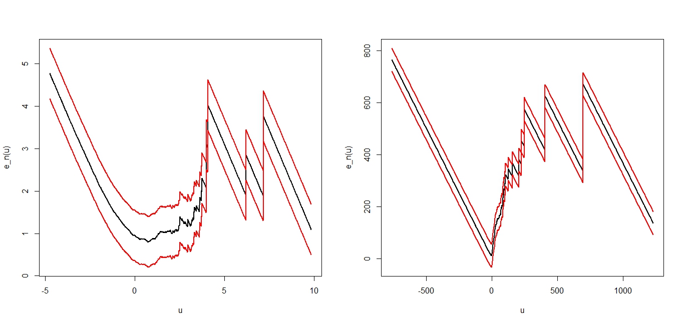
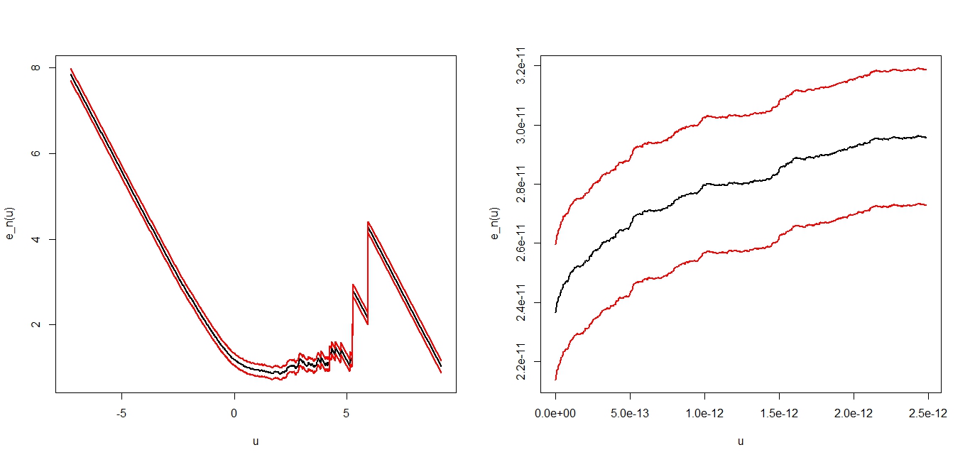
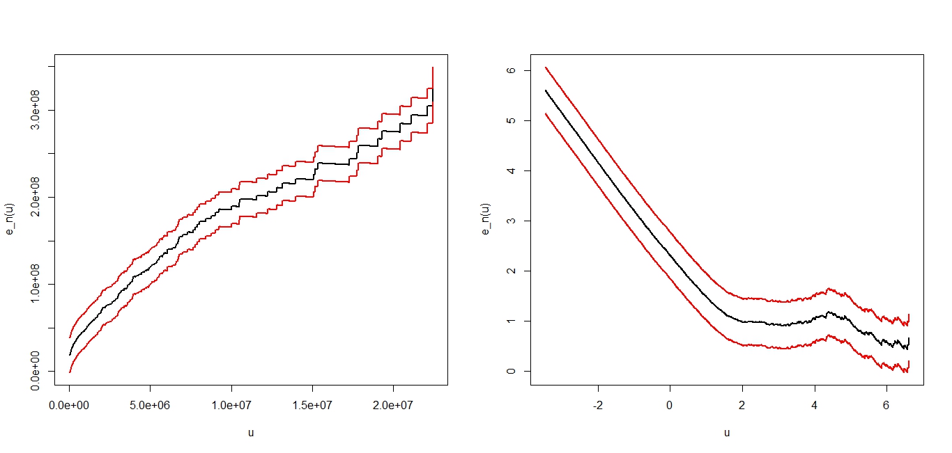
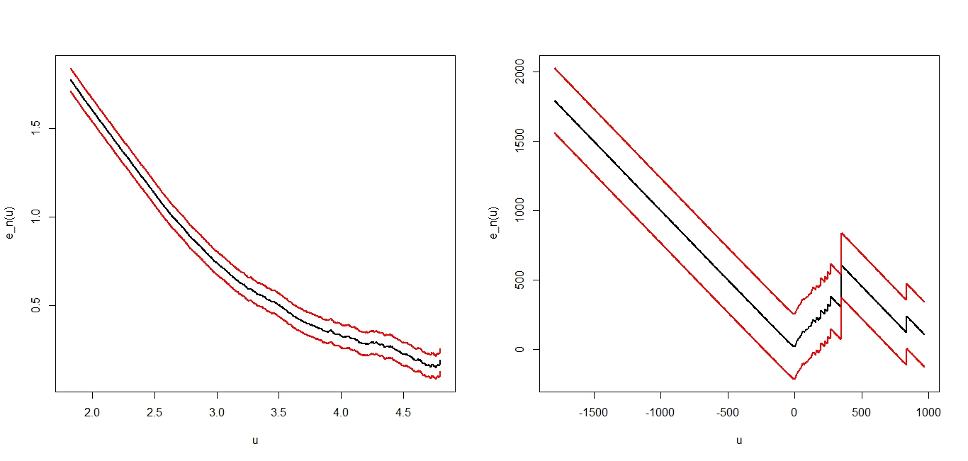
We consider some simple models that are listed in the table 1 below where the used parameters are specified and the emef figures corresponding to each choice are displayed.

Distributions Parameters Figures
GPD ξ=0.25\xi=0.25, β=1\beta=1
ξ=−0.75\xi=-0.75, β=1\beta=1 Figure 1
Pareto α=7,\alpha=7, λ=3\lambda=3
Exponential λ=2\lambda=2 Figure 2
Weibull β=1,τ=3.6\beta=1,\,\tau=3.6
β=1.5,τ=0.2\beta=1.5,\,\tau=0.2 Figure 3
Burr α=0.5,λ=0.5,τ=5\alpha=0.5,\,\lambda=0.5,\,\tau=5
Gomberz α=1,λ=0.5\alpha=1,\,\lambda=0.5 Figure 4
Gamma α=2,β=0.001\alpha=2,\,\beta=0.001
Beta λ=7,β=2\lambda=7,\beta=2 Figure 5
Lognormal μ=0,σ=1\mu=0,\sigma=1
Normal μ=0,σ=1\mu=0,\sigma=1 Figure 6
Laplace μ=0,σ=1,τ=0.5\mu=0,\,\sigma=1,\,\tau=0.5 Figure 7
tt Student ν=5,μ=1\nu=5,\mu=1
Cauchy μ=0\mu=0, δ=1\delta=1 Figure 8
Table 1. The emef for standard distributions
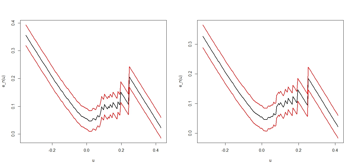
Refer to caption
Figure 1. The emef for two generalized Pareto distributions : the left panel concerns the one with the parameters ξ=0.25,β=1\xi=0.25,\,\beta=1 and the right panel concerns the one with the parameters ξ=−0.75,β=1\xi=-0.75,\,\beta=1.
Refer to caption
Figure 2. The left panel is the emef for a Pareto distribution with the parameters α=7\alpha=7 and λ=3\lambda=3 and the right panel is the one for an Exponential distribution with the parameter λ=2\lambda=2.
Refer to caption
Figure 3. The emef for two Weibull distributions. The left panel concerns the one with the parameters β=1,τ=3.6\beta=1,\,\tau=3.6 and the right panel concerns the one with the parameters
β=1.5,τ=0.2\beta=1.5,\,\tau=0.2.
Refer to caption
Figure 4. The left panel is the emef for the Burr distribution with the parameters α=0.5,λ=0.5,τ=5\alpha=0.5,\,\\ \lambda=0.5,\,\tau=5 and the right one is the emef for the Gomberz distribution with the parameters α=1,λ=0.5\alpha=1,\,\lambda=0.5.
Refer to caption
Figure 5. The left panel is the emef for the Gamma distribution with the parameters α=2,β=0.001\alpha=2,\,\beta=0.001 and the right one is the emef for the Beta distribution with the parameters λ=7,β=2\lambda=7,\beta=2.
Refer to caption
Figure 6. The left panel is the emef for the Lognormal distribution with mean μ=0\mu=0 and with variance σ2=1\sigma^{2}=1 and the right one is the emef for the Normal distribution with the same parameters.
Refer to caption
Figure 7. Emef for Laplace distribution with the parameters μ=0,σ=1,τ=0.5\mu=0,\sigma=1,\,\tau=0.5
Refer to caption
Figure 8. Emef for a tt Student with ν=5\nu=5 degrees of freedom and skewing parameter μ=0\mu=0 (left panel) and for a Cauchy distribution with location parameter μ=0\mu=0 and scale parameter δ=1\delta=1 (right panel).

5.2.2. Generalized hyperbolic models

Next, we consider the emefs for the Gh models. We need some definitions. The Lebesgue density function of the one dimensional Gh is given by

(5.2) fλ,α,β,δ,μ​(x)\displaystyle f_{\lambda,\alpha,\beta,\delta,\mu}(x) =\displaystyle= a(λ,α,β,δ,μ)×(δ2+(x−μ)2)(λ−12)/2​eβ⁡(x−u)×Kλ−12​(α​δ2+(x−μ)2)\displaystyle\textbf{a}_{(\lambda,\alpha,\beta,\delta,\mu)}\times\Big(\delta^{2}+(x-\mu)^{2}\Big)^{(\lambda-\frac{1}{2})/2}e^{\beta(x-u)}\times K_{\lambda-\frac{1}{2}}(\alpha\sqrt{\delta^{2}+(x-\mu)^{2}})

where

a(λ,α,β,δ,μ)=(α2−β2)λ22​π​α(λ−12)​δλ​Kλ​(δ​α2−β2)\displaystyle\textbf{a}_{(\lambda,\alpha,\beta,\delta,\mu)}=\frac{(\alpha^{2}-\beta^{2})^{\frac{\lambda}{2}}}{\sqrt{2\pi}\alpha^{(\lambda-\frac{1}{2})}\delta^{\lambda}K_{\lambda}(\delta\sqrt{\alpha^{2}-\beta^{2}})}

is a norming constant to make the curve area equal to 11 and

Kλ​(x)=12​∫0∞yλ−1​exp⁡(−12​x​(y+y−1))​𝑑y,(x>0)\displaystyle K_{\lambda}(x)=\frac{1}{2}\int_{0}^{\infty}y^{\lambda-1}\exp\Big(-\frac{1}{2}x(y+y^{-1})\Big)dy,\ \ (x>0)

is the modified Bessel function of the third kind with index λ\lambda.

The dependence of the parameters λ,α,β,δ,\lambda,\alpha,\beta,\delta, and μ\mu is as follows: α>0\alpha>0 determines the shape, 0≤|β|<α0\leq|\beta|<\alpha the skewness, μ∈ℝ\mu\in\mathbb{R} is a location parameter and δ>0\delta>0 serves for scaling. The parameter λ∈ℝ\lambda\in\mathbb{R} specifies the order KλK_{\lambda} function Bessel that appears in the Gh density function and is used to obtain different subclasses of Gh distribution.

In the following, we summarise the differents domains of possibilities for the parameters

Ifλ<0,(δ>0,|β|≤α),\displaystyle\mbox{If}\ \ \lambda<0,\ \ \big(\delta>0,\ \ \,|\beta|\leq\alpha\big),
ifλ=0,(δ>0,|β|<α),\displaystyle\mbox{if}\ \ \lambda=0,\ \ \big(\delta>0,\ \ \,|\beta|<\alpha\big),
ifλ>0,(δ≥0,|β|<α).\displaystyle\mbox{if}\ \ \lambda>0,\ \ \big(\delta\geq 0,\ \ \,|\beta|<\alpha\big).

An important Gh family aspect is that it embraces many special cases such that Hyperbolic (λ=1\lambda=1), Student-t⁡(λ<0CLOSEt\,(\lambda<0), Variance Gamma (λ>0\lambda>0), and the Normal Inverse Gaussian (NIG) (λ=−0.5\lambda=-0.5) distributions.

It nests also Generalized Inverse Gamma (GIG) distribution defined only by the three parameters λ,α,\lambda,\alpha, and β\beta. An Inverse Gaussian (IG) distribution is a GIG distribution with λ=−0.5\lambda=-0.5 and a Gamma (Γ\Gamma) distribution is also a GIG distribution with β=0\beta=0.

It contains some limiting distributions such as Cauchy distribution with parameters μ\mu and δ\delta (obtained for λ=−0.5\lambda=-0.5 and α=β=0\alpha=\beta=0).

The Gaussian distribution with mean μ\mu and variance σ2\sigma^{2} are obtained for λ=−0.5\lambda=-0.5, for α,δ→∞\alpha,\delta\rightarrow\infty and δα→σ2\frac{\delta}{\alpha}\rightarrow\sigma^{2}.

The Skew-Student tt with ν\nu degrees of freedom is obtained if α=|β|\alpha=|\beta|, then ν=−2​λ>0\nu=-2\lambda>0.

The Student tt distribution is obtained for α=β=0\alpha=\beta=0, μ=0\mu=0 and δ=ν\delta=\sqrt{\nu}. In the special case of hyperbolic distributions (OPENλ=1),\lambda=1), we obtain the skewed Laplace distribution for δ=0.\delta=0.

All of these have been used to model financial returns and log-returns.

In table 2, we consider some specific Gh distributions with the superscript s​p​espe and limiting distributions with the superscript l​mlm. The used parameters are specified and the emef figures corresponding to each choice are displayed.

Distributions Parameters
λ\lambda α\alpha β\beta δ\delta μ\mu Figures
Hyperboliquespe 11 1.51.5 −0.5-0.5 0.750.75 0.20.2
t-Stud.spe −2-2 10−810^{-8} 00 22 00 Figure 9
Asym. t-Stud.spe −1.278-1.278 0.011860.01186 0.011860.01186 0.07660.0766 1.005
−1.247-1.247 0.01480.0148 −0.0147-0.0147 0.0760.076 1.0051.005 Figure 10
NIGspe -0.5 8.03 -1.37 0.051 0.0105
-0.5 7.6 -1.24 0.052 0.0103 Figure 11
Variance Gammaspe 22 0.3 0.1 2 0
G​I​Gs​p​eGIG^{spe} 55 33 11 - - Figure 12
I​GIG Inverse Gaussianlm 0.50.5 11 00 11 00
Gamma(α,β)l​m(\alpha,\beta)^{lm} 0.5 4.5 10124.5\,10^{12} 10−810^{-8} - - Figure 13
I​ΓI\Gamma Inverse Gammalm −0.5-0.5 1.9×10−81.9\times 10^{-8} 3.1×10−33.1\times 10^{-3} - -
Skew Laplacelm 11 1.11.1 0.10.1 0.0010.001 22 Figure 14
Gaussianlm(OPEN3,0.3)3,0.3) −0.5-0.5 10610^{6} 2 3×1053\times 10^{5} 3
Cauchylm (7,1)(7,1) −0.5-0.5 00 00 1 7 Figure 15
Table 2. Specific and limiting GH distributions.
Refer to caption
Figure 9. Left panel : Emef for an hyperbolic distribution with the parameters λ=1\lambda=1, α=1.5\alpha=1.5, β=−0.5\beta=-0.5, δ=0.75\delta=0.75, μ=0.2\mu=0.2. Right panel : Emef for a tt-student with the parameters λ=−2\lambda=-2, α=10−8\alpha=10^{-8}, β=0\beta=0, δ=2\delta=2, μ=0\mu=0.
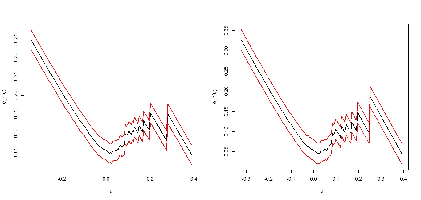
Refer to caption
Figure 10. The emef for two tt-Student distribution. The left panel concerns the one with the parameters λ=−1.278\lambda=-1.278, α=0.01186\alpha=0.01186, β=0.01186\beta=0.01186, δ=0.0766\delta=0.0766, μ=1.005\mu=1.005 and the right panel concerns the one with the parameters λ=−1.247\lambda=-1.247, α=0.0148\alpha=0.0148, β=−0.0148\beta=-0.0148, δ=0.07683\delta=0.07683, μ=1.005\mu=1.005.
Refer to caption
Figure 11. The emef for two Normal Inverse Gaussian distributions. The left panel concerns the one with the parameters λ=−0.5\lambda=-0.5, α=8.03\alpha=8.03, β=−1.37\beta=-1.37, δ=0.051\delta=0.051, μ=0.0105\mu=0.0105 and the right panel concerns the one with the parameters λ=−0.5\lambda=-0.5, α=7.6\alpha=7.6, β=−1.24\beta=-1.24, δ=0.052\delta=0.052, μ=0.0103\mu=0.0103.
Refer to caption
Figure 12. Left panel : the emef for a Variance Gamma distribution with the parameters λ=2\lambda=2, α=0.3\alpha=0.3, β=0.1\beta=0.1, δ=2\delta=2, μ=0\mu=0. Right panel : the emef for a Generalized Inverse Gaussian distribution with the parameters λ=5\lambda=5, α=3\alpha=3, β=1\beta=1.
Refer to caption
Figure 13. Left panel : the emef for Inverse Gaussian distribution with the parameters λ=0.5\lambda=0.5, α=1\alpha=1, β=0\beta=0, δ=1\delta=1, μ=0\mu=0. Right panel : the Emef for a Gamma distribution with the parameters λ=0.5\lambda=0.5, α=4.5×10¹²\alpha=4.5\times 10^{12}, β=10−2\beta=10^{-2}.
Refer to caption
Figure 14. Left panel : the emef for the Inverse Gamma distribution with the parameters
λ=−0.5\lambda=-0.5, α=1.9×10⁻⁸\alpha=1.9\times 10^{-8}, β=3.1×10⁻³.\beta=3.1\times 10^{-3}. Right panel : the emef for the Skew Laplace distribution with the parameters λ=1\lambda=1, α=1.1\alpha=1.1, β=0.1\beta=0.1, δ=10−3\delta=10^{-3}, μ=2\mu=2
Refer to caption
Figure 15. The left panel concerns the emef for the Gaussian distribution with mean μ=2\mu=2 and variance σ2=0.3\sigma^{2}=0.3. The right panel concerns the emef for the Cauchy distribution with location parameter μ=7\mu=7 and scale parameter δ=1\delta=1.

5.2.3. Graphical test

We are now in a position to use the emef graphs already drawn as tools of goodness of fit.

Emef for Normal Inverse Gaussian (NIG) and tt-student-distributions are not monotonic function. They decrease and increase like for emef returns data. For this reason, we fit them to both monthly returns and log-returns from Dow Jones data base (see figure 17, figure 19, figure 21, and figure 23).

Dow Jones data base consists of several compagnies like AXP(American Express compagny), CSCO(Cisco Systems), DAX, CAT, IBM and so one. Each one having 5 values : from opening (op) values to closing (cl) values , also minimum (min), maximum (max), and volume (vol) values.

We select AXP and CSCO compagnies and we consider returns and log-returns for their values as showed in the table 3. Then we construct their emef plot and their fitted counterpart.

Estimates parameters and the emef are given in table 4.

Compagnies Nature Values Emef plots
Real emef Fitted emef
AXP Returns op
min Figure 16 Figure 17
Log-returns. max
cl Figure 18 Figure 19
CSCO Returns min
vol Figure 20 Figure 21
Log-returns op
max Figure 22 Figure 23
Table 3. (Fitted) Emef for DAX and CSCO compagnies data.
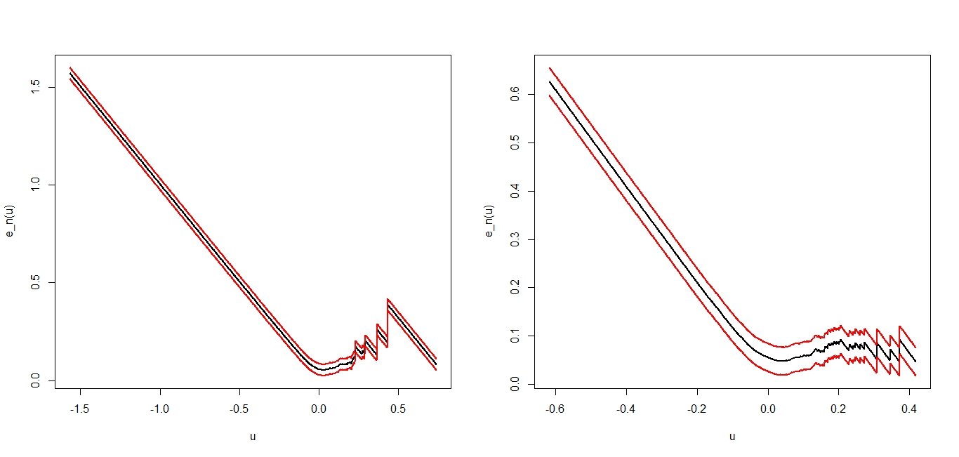
Refer to caption
Figure 16. Emef for AXP compagny (monthly data returns). The left panel concerns the opening values and the right one concerns the minimum values.
Refer to caption
Figure 17. A tt-Student distribution is fitted to monthly data returns for AXP compagny (see figure 16). The left panel concerns a tt distribution with the parameters λ=−1.278,\lambda=-1.278,
α=0.01186,β=0.01186,δ=0.0766,\alpha=0.01186,\beta=0.01186,\delta=0.0766, and μ=1.005\mu=1.005 fitted to opening values.
The right one concerns a tt distribution with the parameters λ=−1.247,α=0.0148\lambda=-1.247,\alpha=0.0148,
β=−0.0148,δ=0.07683,μ=1.005\beta=-0.0148,\delta=0.07683,\mu=1.005 fitted to minimum values.
Refer to caption
Figure 18. Emef for AXP compagny (monthly data log-returns). The left panel concerns the maximum values and the right panel concerns the closing values.
Comp Nature Values Ghyp estimates parameters
λ^\hat{\lambda} α^\hat{\alpha} β^\hat{\beta} δ^\widehat{\delta} μ^\hat{\mu} Fit.Dist Figures
AXP Returns op. −1.278-1.278 0.011860.01186 0.01180.0118 0.07660.0766 1.0051.005 tt-stud
min. -1.247 0.0148 -0.0148 0.0768 1.0051.005 tt-stud Fig. 17
Log-ret. max. -0.5 8.03 -1.37 0.051 0.0105 NIG
cl. -0.5 7.6 -1.24 0.052 0.0103 NIG Fig. 19
CSCO Returns min. -1.24 0.0148 -0.0148 0.0768 1 tt-Stud.
vol. -3.82 4.22 4.22 0.613 0.753 tt-Stud. Fig. 21
Log-ret. op. -1.26 0.83 - 0.83 0.07 0 tt-Stud.
max. -1.32 0.85 -0.85 0.076 0 tt-Stud. Fig. 23
Table 4. Emef for fitted Gh distributions to DAX and CSCO compagnies data.
Refer to caption
Figure 19. A NIG distribution is fitted to monthly data log-returns for AXP compagny (see Figure 18). The left panel concerns the one with the parameters λ=−0.5,α=8.03,\lambda=-0.5,\alpha=8.03,
β=−1.37,δ=0.051,μ=0.0105\beta=-1.37,\delta=0.051,\mu=0.0105 fitted to maximum values. The right panel concerns the one with the parameters λ=−0.5,α=7.6,β=−1.24,δ=0.052,μ=0.0103\lambda=-0.5,\alpha=7.6,\beta=-1.24,\delta=0.052,\mu=0.0103 fitted to closing values.
Refer to caption
Figure 20. Emef for CSCO compagny (data returns). The left panel concerns monthly minimum values and the right panel concerns monthly volum values.
Refer to caption
Figure 21. A tt-student distribution is fitted to monthly data returns for CSCO compagny (see Figure 20). The left panel concerns the one with the parameters λ=−1.24,α=0.014,β=−0.014,δ=0.076,μ=1\lambda=-1.24,\,\alpha=0.014,\\ \beta=-0.014,\,\delta=0.076,\,\mu=1 fitted to minimum values. The right panel concerns the one with the parameters λ=−3.82,α=4.22,β=4.22,δ=0.613,μ=0.753\lambda=-3.82,\,\alpha=4.22,\beta=4.22,\,\delta=0.613,\,\mu=0.753 fitted to volume values.
Refer to caption
Figure 22. Emef for CSCO compagny (data log-returns). The left panel concerns monthly opening values and the right panel concerns monthly maximum values.
Refer to caption
Figure 23. A tt-student distribution is fitted to monthly data log-returns for CSCO compagny (see Figure 22). The left panel concerns the one with the parameters λ=−1.26,α=0.83,β=−0.83,δ=0.07,μ=0\lambda=-1.26,\\ \alpha=0.83,\,\beta=-0.83,\,\delta=0.07,\,\mu=0 fitted to opening values. The right panel concerns the one with the parameters λ=−1.32,α=0.85,β=−0.85,δ=0.076,μ=0\lambda=-1.32,\,\alpha=0.85,\beta=-0.85,\,\delta=0.076,\,\mu=0 fitted to maximum values.

5.2.4. Commentaries

In view of figure 10 and figure 17 we can say that tt studient distribution fits well opening and minimum values return for the American Express compagny AXP, whereas N​I​GNIG distribution fits well maximum and closing log-returns values for the Cysco System compagny CSCO in view of figure 11 and figure 19.

6. Conclusion

In this paper we have established an asymptotic confidence bands for the mean excess function by using functional process approach. Then we applied these bands for fitting Gh distributions to Dowjones financial data. It is a known fact that these ones fit well financial data since they embrace major part of classic distributions.

We remarked that Student and N​I​GNIG distributions are good candidates for fitting returns and log-returns data showing their semi-heavy tails.

7. Appendix

7.1. Moment computations

 
Let Z1,…,Zn,Z_{1},...,Z_{n}, nn i.i.d centered random variables defined on the same probability space with common variance 𝔼⁡(Zi2)=κ1\mathbb{E}(Z_{i}^{2})=\kappa_{1} and common fourth moment 𝔼⁡(Zi4)=κ2>0\mathbb{E}(Z_{i}^{4})=\kappa_{2}>0. We have

(7.1) 𝔼​[T⁡(n,u,δ)]4\displaystyle\displaystyle\mathbb{E}\big[T(n,u,\delta)\big]^{4} =\displaystyle= 𝔼​(Z1+Z2+…​Zn)4\displaystyle\mathbb{E}\Big(Z_{1}+Z_{2}+\ldots Z_{n}\Big)^{4}
=\displaystyle= 𝔼⁡(∑k=1nZk4+6​∑1≤i<j≤nZi2​Zj2)\displaystyle\mathbb{E}\Big(\sum_{k=1}^{n}Z_{k}^{4}+6\sum_{1\leq i<j\leq n}Z_{i}^{2}Z_{j}^{2}\Big)
=\displaystyle= ∑k=1n𝔼⁡(Zk4)+6​∑1≤i<j≤n𝔼⁡(Zi2​Zj2)\displaystyle\sum_{k=1}^{n}\mathbb{E}(Z_{k}^{4})+6\sum_{1\leq i<j\leq n}\mathbb{E}(Z_{i}^{2}Z_{j}^{2})

since, for distinct ii, jj, kk and ll,

𝔼⁡(Zi​Zj3)=𝔼⁡(Zi​Zj2​Zk)=𝔼⁡(Zi​Zj​Zk​Zl)=0,\mathbb{E}(Z_{i}Z_{j}^{3})=\mathbb{E}(Z_{i}Z_{j}^{2}Z_{k})=\mathbb{E}(Z_{i}Z_{j}Z_{k}Z_{l})=0,

by using independence plus the fact that 𝔼⁡(Zi)=0\mathbb{E}(Z_{i})=0.
Using independence again,

𝔼⁡(Zi2​Zj2)=𝔼⁡(Zi2)​𝔼​(Zj2)=κ12fori≠j.\mathbb{E}(Z_{i}^{2}Z_{j}^{2})=\mathbb{E}(Z_{i}^{2})\mathbb{E}(Z_{j}^{2})=\kappa_{1}^{2}\ \ \mbox{for}\ \ i\neq j.

We obtain ∑1≤i<j≤n𝔼⁡(Zi2​Zj2)=n⁡(n−1)2​κ12\displaystyle\sum_{1\leq i<j\leq n}\mathbb{E}(Z_{i}^{2}Z_{j}^{2})=\frac{n(n-1)}{2}\kappa_{1}^{2} since the number of possible couples (i,j)(i,j) of integers such that 1≤i<j≤n1\leq i<j\leq n, is (n2)=n⁡(n−1)2\displaystyle\binom{n}{2}=\frac{n(n-1)}{2}. Hence from (7.1), we deduce that

𝔼​[T⁡(n,u,δ)]4=n​κ2+3​n​(n−1)​κ12.\displaystyle\mathbb{E}\big[T(n,u,\delta)\big]^{4}=n\kappa_{2}+3n(n-1)\kappa_{1}^{2}.

□\square

7.2. Proofs of the uniform asymptotic consistency bounds.

7.2.1. Talagrand bounds

We begin to recall the Talagrand bounds and a device of Einmahl and Mason on how to apply it.
Before going any further, we recall that a class of measurable real valued functions ℱ\mathcal{F} is said to be a pointwise measurable class if there exists a countable subclass ℱ0\mathcal{F}_{0}\ of ℱ\mathcal{F} such as, for any function ff in ℱ\mathcal{F}, we can find a sequence of functions {fm}m≥0\{f_{m}\}_{m\geq 0} in ℱ0\mathcal{F}_{0} for which fm​(x)→f⁡(x)asm→∞f_{m}(x)\rightarrow f(x)\ \ \mbox{as}\ \ m\rightarrow\infty , x∈ℝx\in\mathbb{R}. (See Example 2.3.4 in [10].
Further, let ξ1,ξ2,…\xi_{1},\xi_{2},\ldots be a sequence of independent Rademacher random variables independent of X1,X2,…,X_{1},X_{2},\ldots, and 𝔾m\mathbb{G}_{m} be the functional empirical process indexed by the class of functions ℱ\mathcal{F}.

The following inequality is essentially due to Talagrand (1994) (see [8]).

Inequality. Let ℱ\mathcal{F} be a pointwise measurable class of functions satisfying for some
0<M<∞,‖f‖∞≤M,f∈ℱ,0<M<\infty,\,\|f\|_{\infty}\leq M,\,\ \ f\in\mathcal{F}, .
Then for all t>0t>0 we have,

ℙ{max1≤m≤n∥m𝔾m∥ℱ≥A1(𝔼∥∑i=1nξif(Xi)∥ℱ+t)}\displaystyle\mathbb{P}\Big\{\max_{1\leq m\leq n}\|\sqrt{m}\mathbb{G}_{m}\|_{\mathcal{F}}\geq A_{1}\Big(\mathbb{E}\Big\|\sum_{i=1}^{n}\xi_{i}f(X_{i})\Big\|_{\mathcal{F}}+t\Big)\Big\}
(7.2) ≤ 2(exp(−A2t2/nσℱ2)+exp(−A2t/M)),\displaystyle\ \ \ \ \ \ \ \ \ \ \ \ \ \ \leq\ \ 2\big(\exp(-A_{2}\,t^{2}/n\sigma_{\mathcal{F}}^{2})+\exp(-A_{2}\,t/M)\big),

where σℱ2=supf∈ℱV​a​r​(f⁡(X))\sigma_{\mathcal{F}}^{2}=\sup_{f\in\mathcal{F}}Var(f(X)) and A1,A2A_{1},A_{2} are universal constants.

And the lemma below of Einmahl and Mason [9] is very helpful for obtaining bounds on this quantity, when the class ℱ\mathcal{F} has a polynomial covering number.

Assume that there exists a finite valued measurable function GG, called an envelope function, which satisfies for all x∈ℝ,G⁡(x)≥supf∈ℱ|f⁡(x)|\displaystyle x\in\mathbb{R},\,G(x)\geq\sup_{f\in\mathcal{F}}\left|f(x)\right|. We define for 0<ϵ<10<\epsilon<1

N⁡(ε,ℱ):=supQN⁡(ϵ​Q⁡(G2),ℱ,dQ)N(\varepsilon,\mathcal{F}):=\sup_{Q}N\Big(\epsilon\sqrt{Q(G^{2})},\mathcal{F},d_{Q}\Big)

where the supremum is taken over all probability measures QQ on ℝ\mathbb{R} for which 0<Q⁡(G2):=∫G2​(y)​Q​(𝑑y)<∞0<Q(G^{2}):=\int G^{2}(y)Q(dy)<\infty and dQd_{Q} is the L2​(Q)−L_{2}(Q)-metric. As usual, N⁡(ϵ,ℱ,dQCLOSEN(\epsilon,\mathcal{F},d_{Q}) is the minimal number of balls {g:dQ​(g,f)<ϵ}\{g:d_{Q}(g,f)<\epsilon\} of dQ−d_{Q}-radius ϵ\epsilon needed to cover ℱ\mathcal{F}. Here is the device of Einmahl and Mason [9].

Lemma 3.

(Einmahl - Mason [9]) Let ℱ\mathcal{F} be a pointwise measurable class of bounded functions such that for some constants β>0,ν>0,C>1,σ≤1/(8​C)\beta>0,\,\nu>0,\,C>1,\,\sigma\leq 1/(8C) and function GG as above, the following four conditions hold:

  1. (A.1)

    𝔼⁡[G2​(X)]≤β2;\mathbb{E}\Big[G^{2}(X)\Big]\leq\beta^{2};

  2. (A.2)

    N⁡(ϵ,ℱ)≤C​ε−ν, 0<ϵ<1N(\epsilon,\mathcal{F})\leq C\varepsilon^{-\nu},\ \ 0<\epsilon<1;

  3. (A.3)

    σ02:=supf∈ℱ𝔼⁡[f2​(X)]≤σ2;\displaystyle\sigma_{0}^{2}:=\sup_{f\in\mathcal{F}}\mathbb{E}\Big[f^{2}(X)\Big]\leq\sigma^{2};

  4. (A.4)

    supf∈ℱ‖f‖∞≤12​ν+1​n​σ2/log⁡(β∨1/σ).\displaystyle\sup_{f\in\mathcal{F}}\|f\|_{\infty}\leq\frac{1}{2\sqrt{\nu+1}}\sqrt{n\sigma^{2}/\log(\beta\vee 1/\sigma)}.

Then we have for some absolute constant AA,

(7.3) 𝔼​‖∑i=1nξi​f​(Xi)‖ℱ≤A​ν​n​σ2​log⁡(β∨1/σ).\mathbb{E}\Big\|\sum_{i=1}^{n}\xi_{i}f(X_{i})\Big\|_{\mathcal{F}}\leq A\sqrt{\nu n\sigma^{2}\log(\beta\vee 1/\sigma)}.

7.2.2. APPLICATION

Put ℓu​(x)=ℓ⁡(x)​𝕀(x>u)\ell_{u}(x)=\ell(x)\mathbb{I}_{(x>u)}, with ℓ⁡(x)=1\ell(x)=1 or ℓ⁡(x)=x\ell(x)=x, and let ℱ={ℓu,u∈I}.\mathcal{F}=\{\ell_{u},u\in I\}.
ℱ\mathcal{F} is pointwise measurable since it suffices to take ℱ0={ℓu,u∈I∩ℚ},\mathcal{F}_{0}=\{\ell_{u},u\in I\cap\mathbb{Q}\}, where ℚ\mathbb{Q} is the set of irrationnal numbers.

Next G=max⁡(|ℓ⁡(u0)|,|ℓ⁡(u1)|)=M>0G=\max(\left|\ell(u_{0})\right|,\left|\ell(u_{1})\right|)=M>0 is an envelope of ℱ\mathcal{F} since we have

supu∈I|ℓu​(x)|≤|ℓ⁡(x)|≤max⁡(|ℓ⁡(u0)|,|ℓ⁡(u1)|),∀u0≤x≤u1.\displaystyle\sup_{u\in I}|\ell_{u}(x)|\leq|\ell(x)|\leq\max(\left|\ell(u_{0})\right|,\left|\ell(u_{1})\right|),\quad\forall\,u_{0}\leq x\leq u_{1}.

Remark that if ℓ⁡(x)=1\ell(x)=1 then M=1M=1 and if ℓ⁡(x)=x\ell(x)=x then M=max⁡(|u0|,|u1|).M=\max(|u_{0}|,|u_{1}|).
We have σℱ2=supf∈ℱV​a​r​(f⁡(X))≤M2.\displaystyle\sigma_{\mathcal{F}}^{2}=\sup_{f\in\mathcal{F}}Var(f(X))\leq M^{2}.
So we may use Talagrand’s inequality : it remains to check points of Lemma 3:
Points (A.1) and (A.3) are obvious with β=M=σ.\beta=M=\sigma.
To check (A.2), consider any probability QQ on ℝ.\mathbb{R}. We get for (u,v)∈I2,u≤v,(u,v)\in I^{2},u\leq v,

(7.4) dQ2​(ℓu,ℓv)=∫(ℓu−ℓv)2​(x)​𝑑Q​(x)≤M2​Q​([u,v]).d_{Q}^{2}(\ell_{u},\ell_{v})=\int(\ell_{u}-\ell_{v})^{2}(x)dQ(x)\leq M^{2}Q([u,v]).

By a classical result in probability in ℝ\mathbb{R}, for any given 0<ε<1,0<\varepsilon<1, we may cover [u0,u1][u_{0},u_{1}] by at most
m=⌈u1−u0ε⌉\displaystyle m=\lceil\frac{u_{1}-u_{0}}{\varepsilon}\rceil sub-intervals [si−1,si]\displaystyle[s_{i-1},s_{i}] such that Q([si−1,si])<ε2,i=1,…,m.Q([s_{i-1},s_{i}])<\varepsilon^{2},\ \ i=1,\ldots,m.
(⌈x⌉\lceil x\rceil stands for the smallest positive integer greater than or equal to xx).
Let C=(m+1)​εC=(m+1)\varepsilon, we have m<C​ε−1m<C\varepsilon^{-1}.

For any u∈[u0,u1]u\in[u_{0},u_{1}], there exists i∈{1,…,m}i\in\{1,\ldots,m\} such as si−1≤u≤sis_{i-1}\leq u\leq s_{i} with Q⁡([u,si])<ε2Q([u,s_{i}])<\varepsilon^{2}, so the corresponding ℓu∈ℱ\ell_{u}\in\mathcal{F} is such that

dQ​(ℓu,ℓsi)<ε​M=ε​Q⁡(G2)from (7.4).d_{Q}(\ell_{u},\ell_{s_{i}})<\varepsilon M=\varepsilon\sqrt{Q(G^{2})}\ \ \ \mbox{from \eqref{ent}}.

To finish m=N⁡(ϵ​Q⁡(G2),ℱ,dQ)<C​ε−1m=N\Big(\epsilon\sqrt{Q(G^{2})},\mathcal{F},d_{Q}\Big)<C\varepsilon^{-1} and

N⁡(ϵ,ℱ)=supQN⁡(ϵ​Q⁡(G2),ℱ,dQ)≤C​ε−1.N(\epsilon,\mathcal{F})=\sup_{Q}N\Big(\epsilon\sqrt{Q(G^{2})},\mathcal{F},d_{Q}\Big)\leq C\varepsilon^{-1}.

Now we take β2=σ2=max⁡(2,max⁡(|ℓ⁡(u0)|,|ℓ⁡(u1)|)=M1CLOSE.\beta^{2}=\sigma^{2}=\max(2,\max(\left|\ell(u_{0})\right|,\left|\ell(u_{1})\right|)=M_{1}.
Finally for

n≥8​M2​log⁡M1M12,\displaystyle n\geq\frac{8M^{2}\log M_{1}}{M_{1}^{2}},

we have

(7.5) 𝔼​‖∑i=1nξi​g​(Xi)‖ℱ≤Cℱ​n,\mathbb{E}\Big\|\sum_{i=1}^{n}\xi_{i}g(X_{i})\Big\|_{\mathcal{F}}\leq C_{\mathcal{F}}\sqrt{n},

where Cℱ=A​M1​log⁡M1,\displaystyle C_{\mathcal{F}}=A\,M_{1}\sqrt{\log M_{1}}, since all the points of the Lemma 3 are checked.

Now we are going to apply the inequality (7.2) first for the class of functions

ℱ1={ℓu​(x)=gu​(x),u∈I}.\mathcal{F}_{1}=\{\ell_{u}(x)=g_{u}(x),u\in I\}.

In this case M1=2M_{1}=2 since ℓ⁡(x)=1\ell(x)=1, for any u0≤x≤u1u_{0}\leq x\leq u_{1}, and

𝔼​‖∑i=1nξi​gu​(Xi)‖ℱ1=Dn,1≤Cℱ1​n,whereCℱ1=2​A​log⁡2.\mathbb{E}\Big\|\sum_{i=1}^{n}\xi_{i}g_{u}(X_{i})\Big\|_{\mathcal{F}_{1}}=D_{n,1}\leq C_{\mathcal{F}_{1}}\sqrt{n},\ \ \mbox{where}\ \ C_{\mathcal{F}_{1}}=2A\sqrt{\log 2}.

Let ε>0,n1≥2​log⁡2\varepsilon>0,\,n_{1}\geq 2\log 2 and t0t_{0} such that

exp⁡(−A2​t02n1)≤ε8,andexp⁡(−A2​t0)≤ε8andt0<n1.\exp\Big(\frac{-A_{2}t_{0}^{2}}{n_{1}}\Big)\leq\frac{\varepsilon}{8},\ \ \mbox{and}\ \ \exp\Big(-A_{2}t_{0}\Big)\leq\frac{\varepsilon}{8}\ \ \mbox{and}\ \ \ t_{0}<\sqrt{n_{1}}.

(Remind that σℱ2=1\sigma_{\mathcal{F}}^{2}=1.)
Then

ℙ{max1≤m≤n∥m𝔾m∥ℱ1≥A1(𝔼∥∑i=1nξigu(Xi)∥ℱ1+t0)}≤ε/2.\displaystyle\displaystyle\mathbb{P}\Big\{\max_{1\leq m\leq n}\|\sqrt{m}\mathbb{G}_{m}\|_{\mathcal{F}_{1}}\geq A_{1}\Big(\mathbb{E}\Big\|\sum_{i=1}^{n}\xi_{i}g_{u}(X_{i})\Big\|_{\mathcal{F}_{1}}+\,t_{0}\Big)\Big\}\leq\varepsilon/2.

So for n≥n1,n\geq n_{1}, we arrive at

ℙ⁡(|ℙn​(gu)−ℙX​(gu)|<A1​(Dn,1+t0)n,u∈I)>1−ε/2.\mathbb{P}\Big(\left|\mathbb{P}_{n}(g_{u})-\mathbb{P}_{X}(g_{u})\right|<\frac{A_{1}(D_{n,1}+t_{0})}{n},u\in I\Big)>1-\varepsilon/2.

As t0/n<n1/n≤1t_{0}/\sqrt{n}<\sqrt{n_{1}}/\sqrt{n}\leq 1, we obtain

A1​(Dn,1+t0)n≤A1​Cℱ1​n+A1​nn=A1​Cℱ1+A1n=D1n,\frac{A_{1}(D_{n,1}+t_{0})}{n}\leq\frac{A_{1}C_{\mathcal{F}_{1}}\sqrt{n}+A_{1}\sqrt{n}}{n}=\frac{A_{1}C_{\mathcal{F}_{1}}+A_{1}}{\sqrt{n}}=\frac{D_{1}}{\sqrt{n}},

thus

(7.6) ℙ⁡(|ℙn​(gu)−ℙX​(gu)|<D1n,u∈I)>1−ε/2\mathbb{P}\Big(\left|\mathbb{P}_{n}(g_{u})-\mathbb{P}_{X}(g_{u})\right|<\frac{D_{1}}{\sqrt{n}},u\in I\Big)>1-\varepsilon/2

where D1=2​A​A1​log⁡2+A1D_{1}=2A\,A_{1}\sqrt{\log 2}+A_{1}.

Let us use the same method, for the class of functions

ℱ2={ℓu​(x)=fu​(x),u∈I}.\mathcal{F}_{2}=\{\ell_{u}(x)=f_{u}(x),u\in I\}.

In this case M1=max⁡(2,max⁡(|u0|,|u1|))M_{1}=\max(2,\max(|u_{0}|,|u_{1}|)) since ℓ⁡(x)=x,\ell(x)=x, for any u0≤x≤u1u_{0}\leq x\leq u_{1}, and

𝔼​‖∑i=1nξi​fu​(Xi)‖ℱ2=Dn,2≤Cℱ2​n,whereCℱ2=A​M1​log⁡M1.\mathbb{E}\Big\|\sum_{i=1}^{n}\xi_{i}f_{u}(X_{i})\Big\|_{\mathcal{F}_{2}}=D_{n,2}\leq C_{\mathcal{F}_{2}}\sqrt{n},\mbox{where}\ \ C_{\mathcal{F}_{2}}=AM_{1}\sqrt{\log M_{1}}.

Let n2≥8​M2​log⁡M1M12\displaystyle n_{2}\geq\frac{8M^{2}\log M_{1}}{M_{1}^{2}} and t0t_{0} such that

exp⁡(−A2​t02n2)≤ε8andexp⁡(−A2​t0)≤ε8andt0<n2.\exp\Big(\frac{-A_{2}t_{0}^{2}}{n_{2}}\Big)\leq\frac{\varepsilon}{8}\ \ \mbox{and}\ \ \exp\Big(-A_{2}t_{0}\Big)\leq\frac{\varepsilon}{8}\ \ \mbox{and}\ \ t_{0}<\sqrt{n_{2}}.

Then

ℙ{max1≤m≤n∥m𝔾m∥ℱ2≥A1(𝔼∥∑i=1nξifu(Xi)∥ℱ2+t0)}≤ε/2.\displaystyle\displaystyle\mathbb{P}\Big\{\max_{1\leq m\leq n}\|\sqrt{m}\mathbb{G}_{m}\|_{\mathcal{F}_{2}}\geq A_{1}\Big(\mathbb{E}\Big\|\sum_{i=1}^{n}\xi_{i}f_{u}(X_{i})\Big\|_{\mathcal{F}_{2}}+t_{0}\Big)\Big\}\leq\varepsilon/2.

So for n≥n2,n\geq n_{2}, we deduce that

ℙ⁡(|ℙn​(fu)−ℙX​(fu)|<A1​(Dn,2+t0)n,u∈I)>1−ε/2.\mathbb{P}\Big(\left|\mathbb{P}_{n}(f_{u})-\mathbb{P}_{X}(f_{u})\right|<\frac{A_{1}(D_{n,2}+t_{0})}{n},u\in I\Big)>1-\varepsilon/2.

As t0/n<n1/n≤1t_{0}/\sqrt{n}<\sqrt{n_{1}}/\sqrt{n}\leq 1, we obtain

A1​(Dn,2+t0)n≤A1​Cℱ2​n+A1​nn=A1​Cℱ2+A1n=D2n,\frac{A_{1}(D_{n,2}+t_{0})}{n}\leq\frac{A_{1}C_{\mathcal{F}_{2}}\sqrt{n}+A_{1}\sqrt{n}}{n}=\frac{A_{1}C_{\mathcal{F}_{2}}+A_{1}}{\sqrt{n}}=\frac{D_{2}}{\sqrt{n}},

thus

(7.7) ℙ⁡(|ℙn​(fu)−ℙX​(fu)|<D2n,u∈I)>1−ε/2,\mathbb{P}\Big(\left|\mathbb{P}_{n}(f_{u})-\mathbb{P}_{X}(f_{u})\right|<\frac{D_{2}}{\sqrt{n}},u\in I\Big)>1-\varepsilon/2,

where D2=A​A1​M1​log⁡M1+A1D_{2}=A\,A_{1}\,M_{1}\sqrt{\log M_{1}}+A_{1}.

Now we use again (2.3) :

|en​(u)−e⁡(u)|≤|ℙn​(fu)−ℙX​(fu)|×|ℙn​(gu)|−1+|ℙX​(fu)|×|ℙn​(gu)−ℙX​(gu)||ℙn​(gu)​ℙX​(gu)|.|{e}_{n}(u)-e(u)|\leq|\mathbb{P}_{n}(f_{u})-\mathbb{P}_{X}(f_{u})|\times|\mathbb{P}_{n}(g_{u})|^{-1}\ +\ |\mathbb{P}_{X}(f_{u})|\times\frac{|\mathbb{P}_{n}(g_{u})-\mathbb{P}_{X}(g_{u})|}{|\mathbb{P}_{n}(g_{u})\mathbb{P}_{X}(g_{u})|}.

For u0≤u≤u1u_{0}\leq u\leq u_{1}, we get

0<F¯​(u1)−D1n≤ℙX​(gu)−D1n<ℙn​(gu)<ℙX​(gu)+D1n0<\overline{F}(u_{1})-\frac{D_{1}}{\sqrt{n}}\leq\mathbb{P}_{X}(g_{u})-\frac{D_{1}}{\sqrt{n}}<\mathbb{P}_{n}(g_{u})<\mathbb{P}_{X}(g_{u})+\frac{D_{1}}{\sqrt{n}}

with a probability greater than (w.p.g.t) 1−ε/21-\varepsilon/2 and thus

|ℙn​(gu)|−1<(F¯​(u1)−D1n)−1w.p.g.t​ 1−ε/2\displaystyle|\mathbb{P}_{n}(g_{u})|^{-1}<\Big(\overline{F}(u_{1})-\frac{D_{1}}{\sqrt{n}}\Big)^{-1}\ \ \mbox{{w.p.g.t}}\ \ 1-\varepsilon/2

so we obtain

ℙ(|ℙn(fu)−ℙX(fu)|×|ℙn(gu)|−1<D2n×(F¯(u1)−D1n)−1,u∈I)\displaystyle\mathbb{P}\left(|\mathbb{P}_{n}(f_{u})-\mathbb{P}_{X}(f_{u})|\times|\mathbb{P}_{n}(g_{u})|^{-1}<\frac{D_{2}}{\sqrt{n}}\times\Big(\overline{F}(u_{1})-\frac{D_{1}}{\sqrt{n}}\Big)^{-1},u\in I\right)
≥ℙ⁡(|ℙn​(fu)−ℙX​(fu)|<D2n,u∈I)>1−ε/2,\displaystyle\ \ \ \ \ \ \ \ \ \ \ \ \ \ \ \ \geq\mathbb{P}\Big(\left|\mathbb{P}_{n}(f_{u})-\mathbb{P}_{X}(f_{u})\right|<\frac{D_{2}}{\sqrt{n}},u\in I\Big)>1-\varepsilon/2,

thus

(7.8) ℙ(|ℙn(fu)−ℙX(fu)|×|ℙn(gu)|−1<D2n×(F¯(u1)−D1n)−1,u∈I)>1−ε/2.\mathbb{P}\left(|\mathbb{P}_{n}(f_{u})-\mathbb{P}_{X}(f_{u})|\times|\mathbb{P}_{n}(g_{u})|^{-1}<\frac{D_{2}}{\sqrt{n}}\times\Big(\overline{F}(u_{1})-\frac{D_{1}}{\sqrt{n}}\Big)^{-1},u\in I\right)>1-\varepsilon/2.

From the following inequalities :

{|ℙn​(gu)|−1≤(F¯​(u1)−D1n)−1,w.p.g.t​ 1−ε/2,|ℙX​(gu)|−1≤F¯​(u1)−1,|ℙX​(fu)|≤𝔼​|X|,\begin{cases}\displaystyle|\mathbb{P}_{n}(g_{u})|^{-1}\leq\Big(\overline{F}(u_{1})-\frac{D_{1}}{\sqrt{n}}\Big)^{-1},\ \ \mbox{{w.p.g.t}}\ \ 1-\varepsilon/2,\\ |\mathbb{P}_{X}(g_{u})|^{-1}\leq\overline{F}(u_{1})^{-1},\\ |\mathbb{P}_{X}(f_{u})|\leq\mathbb{E}|X|,\end{cases}

and by the same manner, we obtain

ℙ(|ℙX(fu)|×|ℙn​(gu)−ℙX​(gu)||ℙn​(gu)​ℙX​(gu)|<D1n×𝔼|X|×(F¯(u1)(F¯(u1)−D1n))−1,u∈I)\displaystyle\mathbb{P}\left(|\mathbb{P}_{X}(f_{u})|\times\frac{|\mathbb{P}_{n}(g_{u})-\mathbb{P}_{X}(g_{u})|}{|\mathbb{P}_{n}(g_{u})\mathbb{P}_{X}(g_{u})|}<\frac{D_{1}}{\sqrt{n}}\times\mathbb{E}|X|\times\Big(\overline{F}(u_{1})(\overline{F}(u_{1})-\frac{D_{1}}{\sqrt{n}})\Big)^{-1},u\in I\right)
≥ℙ⁡(|ℙn​(gu)−ℙX​(gu)|<D1n,u∈I)>1−ε/2,\displaystyle\ \ \ \ \ \ \ \ \ \ \ \ \ \ \ \ \geq\mathbb{P}\Big(\left|\mathbb{P}_{n}(g_{u})-\mathbb{P}_{X}(g_{u})\right|<\frac{D_{1}}{\sqrt{n}},u\in I\Big)>1-\varepsilon/2\,,

thus

(7.9) ℙ⁡(|ℙX​(fu)|×|ℙn​(gu)−ℙX​(gu)||ℙn​(gu)​ℙX​(gu)|<D1n×𝔼​|X|×(F¯​(u1)​(F¯​(u1)−D1n))−1)>1−ε/2\mathbb{P}\left(|\mathbb{P}_{X}(f_{u})|\times\frac{|\mathbb{P}_{n}(g_{u})-\mathbb{P}_{X}(g_{u})|}{|\mathbb{P}_{n}(g_{u})\mathbb{P}_{X}(g_{u})|}<\frac{D_{1}}{\sqrt{n}}\times\mathbb{E}|X|\times\Big(\overline{F}(u_{1})(\overline{F}(u_{1})-\frac{D_{1}}{\sqrt{n}})\Big)^{-1}\right)>1-\varepsilon/2

By combining (7.8) and (7.9), we obtain

ℙ(|ℙn(gu)|−1×|ℙn(fu)−ℙX(fu)|≥D2n×(F¯(u1)−D1n)−1,u∈I)\displaystyle\mathbb{P}\left(|\mathbb{P}_{n}(g_{u})|^{-1}\times\left|\mathbb{P}_{n}(f_{u})-\mathbb{P}_{X}(f_{u})\right|\geq\frac{D_{2}}{\sqrt{n}}\times\Big(\overline{F}(u_{1})-\frac{D_{1}}{\sqrt{n}}\Big)^{-1},u\in I\right)
+ℙ⁡(|ℙX​(fu)|×|ℙn​(gu)−ℙX​(gu)||ℙn​(gu)​ℙX​(gu)|≥D1n×𝔼​|X|×(F¯​(u1)​(F¯​(u1)−D1n))−1)\displaystyle\ \ \ \ \ \ \ \ \ \ \ \ \ \ \ \ \ +\ \ \ \mathbb{P}\left(|\mathbb{P}_{X}(f_{u})|\times\frac{|\mathbb{P}_{n}(g_{u})-\mathbb{P}_{X}(g_{u})|}{|\mathbb{P}_{n}(g_{u})\mathbb{P}_{X}(g_{u})|}\geq\frac{D_{1}}{\sqrt{n}}\times\mathbb{E}|X|\times\Big(\overline{F}(u_{1})(\overline{F}(u_{1})-\frac{D_{1}}{\sqrt{n}})\Big)^{-1}\right)
≤ε2+ε2≤ε.\displaystyle\ \ \ \ \ \ \ \ \ \ \ \ \ \ \ \ \ \leq\ \ \ \frac{\varepsilon}{2}\ \ \ \ +\ \ \ \ \frac{\varepsilon}{2}\ \ \ \ \leq\ \ \ \ \varepsilon\,.

This gives

ℙ⁡(|en​(u)−e⁡(u)|≥Enn)≤εwhereEn=1F¯​(u1)−D1/n​(D2+D1×𝔼​|X|F¯​(u1)).\mathbb{P}(|e_{n}(u)-e(u)|\geq\frac{E_{n}}{\sqrt{n}})\leq\varepsilon\ \ \ \mbox{where}\ \ \ E_{n}=\frac{1}{\overline{F}(u_{1})-D_{1}/\sqrt{n}}\Big(D_{2}+\frac{D_{1}\times\mathbb{E}|X|}{\overline{F}(u_{1})}\Big).

Finally we conclude by :

ℙ(en(u)−Enn<e(u)<en(u)+Enn,u∈I)>1−ε\mathbb{P}\Big(e_{n}(u)-\frac{E_{n}}{\sqrt{n}}<e(u)<e_{n}(u)+\frac{E_{n}}{\sqrt{n}},u\in I\Big)>1-\varepsilon

for any ε>0\varepsilon>0, any n≥n0n\geq n_{0} with

En=1F¯​(u1)−D1/n​(D2+D1×𝔼​|X|F¯​(u1))and{D1=2​A​A1​log⁡2+A1D2=A​A1​M1​log⁡M1+A1,M1=max⁡(2,max⁡(|u0|,|u1|))E_{n}=\frac{1}{\overline{F}(u_{1})-D_{1}/\sqrt{n}}\Big(D_{2}+\frac{D_{1}\times\mathbb{E}|X|}{\overline{F}(u_{1})}\Big)\ \ \ \mbox{and}\ \ \ \ \ \left\{\begin{array}[]{l}\displaystyle D_{1}=2AA_{1}\sqrt{\log 2}+A_{1}\cr\displaystyle D_{2}=A\,A_{1}\,M_{1}\sqrt{\log M_{1}}+A_{1},\cr M_{1}=\max(2,\max(|u_{0}|,|u_{1}|))\cr\end{array}\right.

□\square

References

  • [1] Alexander J. McNeil, Rudiger Frey &\& Paul Embrechts (2005). Quantitative Risk Management: Concepts, Techniques, and Tools. Princeton University Press.
  • [2] Billingsley, Patrick (1968). Convergence of Probability measures. John Wiley, New-York.
  • [3] Grace L. Yang (1978). Estimation Of biomedical function, The Annals of Statistics, Vol.6, No.1, 112-116.
  • [4] Guess, F., Proschan, F., (1988). Mean residual life. In: Rao Krishnaiah, P.R., Rao, C.R. (Eds.), Handbook of Statistics,Vol.7. North-Holland, Amsterdam, pp. 215-224.
  • [5] Hall, W.J. and Wellner, J.A.(1981). Mean residual life.. In: Csorgo, M.,Dawson, D.A., Rao, J.N.K., Saleh, A.K.Md.E.( Eds), Statistics and Related Topics. North-Holland, Amsterdam, pp. 169-184.
  • [6] Kotz,S., Shanbhag, D.N., (1980). Some new approaches to probability distributions . Adv. in Appl. Probab. 12, 903-921.
  • [7] Lo, G.S.(2014) A remark on the asymptotic tightness in ℓ+∞​([a,b])\ell^{+\infty}([a,b]). arxiv.org/pdf/1405.6342.
  • [8] M. Talagrand (1994) Sharper bounds for gaussian and empirical processes, The Annals of Probability, Vol. 22, No. 1,28-76. University of Paris VI and Ohio State University.
  • [9] Uwe Einmahl and David M.Mason (2005). Uniform in bandwidth consistency of Kernel-Type function estimators, The Annals of Statistics , Vol. 33, No. 3, 13801403.
  • [10] Van Der Vaart, A. W. and Wellner, J. A. (1996). Weak convergence and empirical processes with application in statistcs, ISBN 0-387-94640-3 Springer-Verlag New York Berlin Heidelberg.