On the Combined Analysis of Muon Shower Size and Depth of Shower Maximum
Abstract:
The mass composition of ultra-high energy cosmic rays can be studied from the distributions of the depth of shower maximum and/or the muon shower size. Here, we study the dependence of the mean muon shower size on the depth of shower maximum in detail. Air showers induced by protons and iron nuclei were simulated with two models of hadronic interactions already tuned with LHC data (run I-II). The generated air showers were combined to obtain various types of mass composition of the primary beam. We investigated the shape of the functional dependence of the mean muon shower size on the depth of shower maximum and its dependency on the composition mixture. Fitting this dependence we can derive the primary fractions and the muon rescaling factor with a statistical uncertainty at a level of few percent. The difference between the reconstructed primary fractions is below 20% when different models are considered. The difference in the muon shower size between the two models was observed to be around 6%.
30 July - 6 August, 2015
The Hague, The Netherlands
1 Introduction
The mass composition of ultra–high energy cosmic rays (UHECR) inducing extensive air showers of energies above eV can be measured by fluorescence detectors on average basis. The measurement of the depth of shower maximum () is compared with Monte Carlo (MC) predictions in such cases [1, 2]. The fluorescence technique provides a precise measurement of , but a large systematic uncertainty remains in the determination of the mass composition of UHECR. The obstacle comes predominantly from different predictions of hadronic interaction models that are extrapolated from accelerator energies to energies larger by a few orders of magnitude in the center of mass system. The mass composition of UHECR remains uncertain, and even unknown at the highest energies where a steep decrease of the flux is observed [3, 4]. The very low statistics of events collected by fluorescence detectors is due to their low duty cycle.
Assuming a small number of primaries to be present in UHECR, the most probable fractions of these primaries were inferred in [5]. The measured distributions of were compared with distributions by combining MC distributions of the assumed primaries. Large differences in the results were found among the hadronic interaction models. Also, a degeneracy of solutions with similar probability can be expected as, generally, there are many combinations of MC distributions of the individual primaries which describe the measured distributions similarly well.
Whereas the fluorescence technique measures the longitudinal profile of the electromagnetic component of the shower, a measurement of the number of muons on the ground () can provide an independent way to infer the mass composition of UHECR. Muon detectors have a 100% duty cycle and, when a good resolution of is achieved (10%), even better separability of the individual primaries can be achieved than in the case of the fluorescence technique. However, there is a lack of in MC simulations when compared with the measured data [6, 7, 8]. The underestimation of muon production is usually characterized in terms of a muon rescaling factor. Moreover, a stronger relationship between and the shower energy than between and the shower energy [9] makes the situation more difficult and an independent measurement of the shower energy is needed for composition studies using . Therefore a simple comparison of the measured distributions of muons with MC predictions would be complicated.
A combined measurement of UHECR showers with the fluorescence technique ( and shower energy) and muon detectors () could be a more sucessfull way to determine the mass composition of UHECR. In the previous studies, the detected muon and electromagnetic signals were utilized to determine the average mass number of a set of air showers, see e.g. [10]. There are also methods estimating the spread of masses in the UHECR primary beams via correlation of and [11] or from signals in muon and electromagnetic detectors [12]. However, it needs to be mentioned that the two currently operating experiments do not yet directly measure the muonic component for showers with zenith angles below 60∘.
Here we present another method to determine the fractions of the assumed primaries in which the rescaling of () can be achieved simultaneously with a single fit of a combined measurement of and . For this purpose we use MC showers generated with two hadronic interaction models tuned to the LHC data (run I-II).
In the next section, the generated showers that were used in this work are described. The method to determine the fractions of the assumed primaries and is introduced in Section 3. Section 4 contains applications of the method on several examples, testing its performance. The work is summarized in the last section.
2 Simulated Showers
For this work we have simulated showers with the CONEX 4.37 generator [13, 14] for p and Fe primaries with fixed energy eV and for each of the two hadronic interaction models (QGSJet II–04 [15] and EPOS–LHC [16, 17]). The zenith angles () of showers were distributed uniformly in for in .
Muons with threshold energy 300 MeV at 1400 m a.s.l. were included to calculate . Electromagnetic particles of energies above 1 MeV formed the longitudinal profile (dependence of the deposited energy on the atmospheric depth), from which was fitted with the Gaisser–Hillas function by the program CONEX.
For each shower we used Gaussian smearing of and with a variance equal to and , respectively. These smearings imitate the detector resolutions. We adopted a correction for the attenuation of with zenith angle due to the different amount of atmosphere penetrated by the air shower before it reaches the ground. The correction was made using a polynomial of 3rd order in for each model of hadronic interactions. An equally mixed composition of p and Fe was considered for this purpose.


3 Method


For both hadronic interaction models, we parametrized distributions with Gumbel functions [18] (see Fig. 1) for both primaries = p, Fe. We also parametrized the dependence of mean , , on with quadratic functions in denoted as (see Fig. 2), again for both primaries. We introduced the rescaling factor of to incorporate into the method the case when a rescaling of obtained from MC is needed to fit the measured . Then, for a combination of two primaries with fractions , , is given as
| (1) |
where the weights are expressed as
| (2) |
For each bin of , is calculated as the weighted average of rescaling both with the same factor . The weights reflect the relative contribution of each individual primary with relative fraction in each bin of according to .
Thus, any given dependence of on , which is similar to the dependence of combined proton and iron showers, can be fitted with the two–parameter ( and ) fit. The Fe fraction is obtained afterwards as .
An example of application of the method to the mixed composition of showers initiated with 50% p and 50% Fe is shown in Fig. 3. The fitted dependence of on (black points) is shown with the gray dashed line. The hadronic interaction model EPOS–LHC was considered. Starting from the lowest values of , matches to about 650 g/cm2 where a transition towards begins. It continues up to about 800 g/cm2 where starts to match .

4 Application of Method
In this section we show basic examples of the present method and rough estimates how accurately the primary fractions of p and Fe and the muon rescaling factor can be determined. In the following, we assumed the detector resolutions to be g/cm2 and %. We considered 11 combinations of mixed compositions of p and Fe with fractions in steps of 10% for both hadronic interaction models. Each of these compositions was reconstructed with each of the two parametrizations obtained for the two hadronic interaction models. Additionally, we reconstructed an example dataset with parametrizations of each of the two models to have another assessment of the method with respect to the two models.
On the left panel of Fig. 4, a comparison of the fitted and the true proton fraction is shown for QGSJet II–04 (blue) and EPOS–LHC (red). The reconstructed of showers generated with a different model than that used for the parametrization of and are depicted by open black markers. Scenario 1 (2) corresponds to showers produced with QGSJet II–04 (EPOS–LHC) and fitted with the parametrizations obtained from EPOS–LHC (QGSJet II–04) showers.
When the same hadronic interaction model is used for the generation of showers and parametrization of and , the proton fraction is reconstructed within a few % of the true value. However, in cases of Scenario 1 and 2, the difference between the fitted and the true proton fraction increases with the spread of primary masses of the selected composition. It reaches values up to 20%.


On the right panel of Fig. 4, the muon rescaling is plotted for different true proton fractions. The rescaling factor is found to be within a few % to 1 (precision of the method), when the same models were used for parametrization and generation (red and blue). Black points correspond to the relative difference of for showers generated with QGSJet II–04 and EPOS–LHC, which is about 6%.
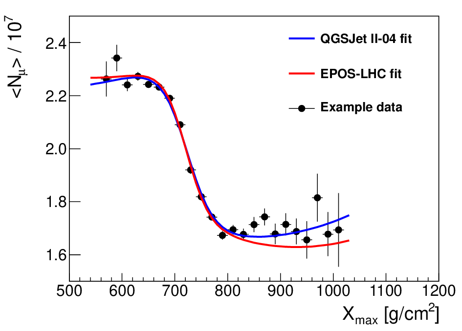
As another check, we created example data from 5000 p and 5000 Fe showers produced with QGSJet II–04. For each shower, we scaled by a factor 1.3 and increased by 7 g/cm2. Note that EPOS–LHC generates showers with deeper than QGSJet II–04 by about 14 g/cm2 on average. These example data were fitted with parametrizations of both models (see Fig. 5). Both fits describe the example data similarly well giving different proton fractions and muon rescaling factors that are shown in Tab. 1. The difference of is about 15% when different parameterizations (Figs. 1,2) based on two most recent models are used. The ratio of for the two models reflects again that EPOS–LHC produces about 6% more muons than QGSJet II–04 on average.
| Model | [%] | |
|---|---|---|
| QGSJet II–04 | 41 2 | 1.297 0.004 |
| EPOS–LHC | 56 2 | 1.216 0.004 |
5 Conclusions
A method of simultaneously obtaining the primary fractions and the muon rescaling factor from and of UHECR was presented. Simulated showers with two models of hadronic interactions tuned to LHC data (run I-II) were used. The precision of the method was tested with different combinations of p and Fe primaries and with example data. The primary fractions and the muon rescaling factor can be determined within a few %. The difference of the proton fraction reconstructed with the two parameterizations based on the two models of hadronic interactions was observed below 20%. The muon rescaling factor reflected the relative difference (around 6%) in the average muon shower size of the two models of hadronic interactions.
Acknowledgements
This work is funded by the Czech Science Foundation grant 14-17501S.
References
- [1] A. Aab et al. (The Pierre Auger Collaboration), Phys. Rev. D 90 (2014) 122005.
- [2] R. U. Abbasi et al. (Telescope Array Collaboration), Astropart. Phys. 64 (2014) 49-62.
- [3] J. Abraham et al. (The Pierre Auger Collaboration), Phys. Rev. Lett. 101 (2008) 061101.
- [4] T. Abu-Zayyad et al. (Telescope Array Collaboration), ApJ 768 (2013) L1.
- [5] A. Aab et al. (The Pierre Auger Collaboration), Phys. Rev. D 90 (2014) 122006.
- [6] A. Aab et al. (The Pierre Auger Collaboration), JCAP 8 (2014) 019.
- [7] B. Kegl for the Pierre Auger Collaboration, Proc. of the 33rd ICRC 2013, arXiv:1307.5059 [astro-ph.HE].
- [8] G. R. Farrar for the Pierre Auger Collaboration, Proc. of the 33rd ICRC 2013, arXiv:1307.5059 [astro-ph.HE].
- [9] J. Mathews, Astropart. Phys. 22 (2005) 387-397.
- [10] P. Luczak et al., Proc. of the 33rd ICRC 2013, arXiv:1308.2059 [astro-ph.HE].
- [11] P. Younk & M. Risse, Astropart. Phys. 35 (2012) 807-812.
- [12] J. Vicha et al., Astropart. Phys. 69 (2015) 11-17.
- [13] T. Bergmann et al., Astropart. Phys. 26 (2007) 420-432.
- [14] T. Pierog et al., Nucl. Phys. B. - Proc. Suppl. 151 (2006) 159-162.
- [15] S. S. Ostapchenko, Phys. Rev. D 83 (2011) 014018.
- [16] K. Werner, F. M. Liu and T. Pierog, Phys. Rev. C 74 (2006) 044902.
- [17] T. Pierog and K. Werner, Nucl. Phys. B - Proc. Suppl. 196 (2009) 102-105.
- [18] E. J. Gumbel, Statistics of extremes, Dover Publications (2004).