Compiled August 24, 2026 \ociscodes(220.1010) Aberrations, (080.0080) Geometric Optics
Ray and Wave Aberrations Revisited: A Huygens-Like Construction Yields Exact Relations
Abstract
The aberrations of an optical system can be described in terms of the wave aberrations, defined as the departure from the ideal spherical wavefront; or the ray aberrations, which are in turn the deviations from the paraxial ray intersections measured in the image plane. The classical connection between the two descriptions is an approximation, the error of which has, so far, not been quantified analytically. We derive exact analytical equations for computing the wavefront surface, the aberrated ray directions, and the transverse ray aberrations in terms of the wave aberrations (OPD) and the reference sphere. We introduce precise conditions for a function to be an OPD function, show that every such function has an associated wavefront, and study the error arising from the classical approximation. We establish strict conditions for the error to be small. We illustrate our results with numerical simulations. Our results show that large numerical apertures and OPD functions with strong gradients yield larger approximation errors.
1 Introduction
The geometrical theory of aberrations adjusts the predictions of paraxial optics to a more realistic depiction of how a real lens performs. Two of its descriptors are the ray aberrations and the wave aberrations. Both concepts are directly related, as has been shown in the classic literature [1, 2, 3, 4]. The ray aberrations describe the deviation between the aberrated rays and the paraxial/ideal rays as a transverse distance measured in the image plane. The wave aberration describes the deviation of the aberrated wavefront as compared to an ideal spherical wavefront that produces a perfect image point. Equivalently, one can consider the wave aberrations as the differences in time of flight of the light along an aberrated ray with respect to the time it would take to reach the image along a paraxial ray, hence the alternative use of the name optical path differences (OPD).
| (1) |
where represents the wave aberration (OPD), and are the ray aberrations, and is the radius of the ideal wavefront, also known as the reference sphere.
The approximation in Eqs. (1) is commonly held to be valid for small numerical apertures and small aberrations. In spite of this, they are widely used for instance in the analysis of the Hartmann-Shack sensor [6, 7] or in optical design software.
While exact relations between quantities indirectly related to the aberrations [8], or based on re-definitions of the optical path difference [9], have appeared in the literature, there is, so far, no such relation for the standard definition of the optical path difference as a phase difference along the aberrated ray.
In this paper, we derive exact analytical equations to compute wavefront points, aberrated ray directions and the transverse ray aberrations in terms of the OPD function along the aberrated ray. Whereas the classical equations, Eqs. (1), are only an approximation, the new equations are applicable to large numerical aperture settings and for arbitrary differentiable OPD functions. We prove the exactness of the equations by validating the defining properties of the wavefront, i.e. the distance to the reference sphere and the orthogonality with the aberrated rays. We show that the classical equations for the ray aberrations are a special case of our equations and detail the conditions for a good approximation. Finally, we evaluate the approximation error quantitatively.
2 Overview
The main tool for our derivation is a Huygens-like interpretation of the wavefront as an envelope of spheres with a varying radius that is given by the OPD function, Fig. 2a.
This conception enables us to perform limit considerations that are most suitably studied in the tangent space of the reference sphere. The derivations are initially performed in this local space rather than in exit pupil coordinates. In the new coordinate system, we arrive at exact analytic equations for the wavefront and the aberrated ray directions, which, by means of a suitable transformation can be related to the original exit pupil coordinates. In this scheme, the aberrated ray directions can be computed without differentiating the wavefront.
As a result, we obtain a set of rays with origins at the wavefront that can be propagated to the image plane to compute the exact analytic expressions for the transverse ray aberrations.
We perform the derivation in several steps. First, Sect. 4, we perform the basic geometric construction of a wavefront tangent in one dimension in the canonical setting afforded by the tangent space construction outlined above.
We leave the detailed definition of the required coordinate transformation for the discussion of the two-dimensional case, Sect. 5. We introduce the transformation between global and local coordinate frames, putting special emphasis on the transformation of functions defined in global exit pupil coordinates to the local tangent frame systems.
We then generalize the one-dimensional geometric argument to two dimensions, Sect. 6, and derive local expressions for the wavefront and the aberrated ray directions. We continue by linking these expressions back to exit pupil coordinates, both in their arguments and in their values. We arrive at the key results, Eqs. (6.2) and (81).
Finally, we make a connection to the transverse ray aberrations and the classical approximation, Eqs. (1), elucidating the conditions for a valid approximation. Sect. 8 demonstrates exemplary applications and quantitative properties of the equations.
The Appendix contains a proof of the wavefront properties of the derived quantities and establishes that every OPD function corresponds to a wavefront.
3 The Wave Aberration Function (OPD)
3.1 OPD Definitions
In the classic literature, there are two different recurrent definitions for the wave aberration function (OPD).
The standard definition [1, 5, 3] considers the path length between points on the aberrated wavefront and on the reference sphere, connected along the direction of the propagation of the aberrated ray. The OPD value is reported for the coordinate of the reference sphere point in the exit pupil plane. Its relation to the ray aberration is stated in Eqs. (1).
The alternative definition [9, 3] considers the wave aberration to be measured along a radius of the reference sphere, again between two points on the wavefront and on the reference sphere, but with the OPD value assigned to the exit pupil location of the wavefront point.
Both definitions are illustrated in Fig. 1 for a point on the wavefront. For simplicity, we refer to the first definition as since the path lengths are measured along the ray, while the second one is denoted as . The pupil coordinate represents the pupil coordinate position for , while is the same for the alternative wave aberration definition. The wave aberration value is given a sign that depends on the delay relation between the wavefront and the reference sphere. For the particular case of point in Fig. 1, the wavefront is delayed which implies a negative sign of the OPD.

For the resulting relation between ray and wave aberration is different from Eqs. (1) and is reported [9] as:
| (2) |
The advantage of the definition is a simple computation of the wavefront surface via triangle relationships. However, Eqs. (2) are differential equations as compared to the classical Eqs. (1) and therefore, even though they are exact [9], difficult to solve.
On the other hand, for the standard definition, , there is no obvious construction of the wavefront surface from the OPD values, since the aberrated ray directions are unknown.
Most authors prefer the definition since it provides a direct connection with the pupil function and the calculation of the point spread function (PSF) [2], but often the distinction is not clearly made.
In this article, we derive exact equations for the wavefront and the aberrated ray directions for the standard OPD definition and use them to make an exact link with the ray aberrations.
3.2 Properties of the OPD Function
Since the derivations critically depend on the exact properties of the OPD definition, we discuss the interpretation underlying our derivations in detail.
We use the standard definition of the OPD function as given above, simply denoting it as in the following. In contrast to most of the literature, we interpret the domain of the OPD function to be the reference sphere. The usual parameterization in terms of exit pupil coordinates is, in this sense, one parameterization of the function’s domain. Other parameterizations are possible and we will use this insight to define the OPD function in local coordinate systems, Sect. 5. These differently parameterized OPD functions all describe the same quantity, i.e. the phase delay along an aberrated ray intersecting the reference sphere at the position of intersection, just with a different frame of reference.
A direct consequence of the above considerations and the fact that the OPD is single-valued is that no wavefront point can be at a closer distance to the reference sphere than the OPD value. This implies that there is an open ball around any point on the reference sphere that does not contain wavefront points. The radius of this open ball is equal to the OPD value. A sphere with this radius, i.e. the closure of the open ball, is tangent to the wavefront. The wavefront can therefore be considered as the envelope of a set of spheres with a varying radius that is described by the OPD function, a statement of Huygens principle. The concept is illustrated in Fig. 2 a), where is the reference sphere, the OPD function, and the resulting wavefront.
A misconception that is often found in the literature is an ambiguity between the slope of the wavefront and the slope of the OPD function. We emphasize that these two concepts must be distinguished.
A key property of an OPD function is that its gradient magnitude cannot exceed one. To appreciate this point, consider a 1D setting, Fig. 2 b) and c). As mentioned above, the OPD value implies an open ball without wavefront points surrounding a particular point on the reference sphere. If the norm of the OPD derivative is greater than one , the radius of this ball changes more quickly than the evaluation position , i.e. . It follows that one of the balls completely contains the other – which is a contradiction since both balls, by definition, do not contain wavefront points, but are simultaneously tangent to it. It follows that the norm of the OPD derivative cannot exceed one. An intuitive interpretation of this property is that the OPD would be required to be multi-valued in this situation. An alternative interpretation is that the wavefront can only be represented as an envelope of balls if the condition on the OPD norm is satisfied.
The illustration in Fig. 2 b) and c) shows the two cases for a finite displacement . The constraint that one ball does not contain the other yields the triangle inequalities illustrated in the Figure. Passing to the limit as yields the condition .
With these prerequisites, we introduce the following
Definition.
OPD function: An OPD function is a twice-differentiable function with a gradient norm smaller or equal to one. Its domain is the reference sphere.
The existence of the second derivatives is a technical requirement for subsequent developments. As implied by the definition, the gradient is to be taken on the reference sphere.
In contrast to the above discussion, the wavefront derivative can have arbitrary values. It follows that there are wavefronts that cannot be represented by an OPD function. However, we show in the Appendix that all OPD functions, satisfying the above conditions, describe wavefronts by deriving explicit construction rules. The specification of an OPD function is therefore a sufficient condition for a wavefront to exist.

4 Wavefront Points and Aberrated Ray Directions in a 1D Canonical Setting
We develop the major geometric reasoning of our derivation in a canonical one-dimensional setting. Without loss of generality, we consider an orthonormal local coordinate system with its origin on the reference sphere and spanning its tangent space. To complete the basis, we use the tangent plane normal, oriented towards the paraxial image point . Such a local coordinate system is depicted in Fig. 3 for the current one-dimensional setting, for the point . In local coordinates , i.e. it coincides with the local coordinate origin.
As detailed in Sect. 5 for the full 2D case, these local coordinate systems can be obtained by a rigid body transformation of the exit pupil coordinate system.
All quantities relating to the local system are denoted with circumflex symbols. In particular, is the local coordinate origin, and are the local coordinate axes and is the OPD function parameterized in local coordinates . The specifics of this parameterization are also covered in Sect. 5 for the 2D-setting. In addition, we denote the local representation of the reference sphere as and the local aberrated ray directions as . Given these quantities, we may express a wavefront point as
| (3) |
where is a point on the reference sphere corresponding to the local tangent space coordinate , see Fig. 3. The local wavefront function yields the local 2D coordinates of the wavefront point. Its horizontal coordinate may be different from the evaluation position .
4.1 Constructing a Tangent to the Wavefront
Considering the fundamental definition of the wavefront as the surface which is normal to the aberrated rays, we can consider a circle with radius that is centered in the point , i.e. in the origin of the local coordinate system. This circle must be tangent to the wavefront since the wavefront is, by definition, located at a distance from point . We wish to determine the point of intersection between the circle and the wavefront.
For this, we introduce a neighboring second circle with its center at point , also centered on the reference sphere and also tangent to the wavefront with radius . Both circles are shown in Fig. 4.
We now consider the circle at to be approaching the circle at the center of the local coordinates . In the limit, as the horizontal distance between the centers tends to zero, the two circles coincide and the tangent to both becomes the tangent of the wavefront. Expressing this intuition mathematically leads to equations for the ray direction and the wavefront itself.

Considering in more detail the geometry of Fig. 4, the tangent to both circles intersects the line connecting their centers at the point , where distances between the points are related by the simple triangle relation
| (4) |
Using we arrive at the following equation
| (5) |
The point is then given by:
| (6) |
We now introduce the explicit expressions for the vector quantities
| (7) |
and insert the definitions into Eq. (6). We use a Taylor expansion for at the point for studying the limit as point approaches point . Since the OPD function is differentiable, the relation is exact in this limit. We thus obtain an explicit equation for the vector
| (8) |
which, as tends to zero becomes
| (9) |

where the limit has been determined using the rule of . The previous equation is illustrated in Fig. 5. The limit behavior of the point is finite if and it is located on the axis. For the case that , the point is located at infinity. However the calculation of the wavefront point is now trivial since it is located on the axis at a distance from the origin of the local coordinates.
For the limiting case where is finite, we determine the tangent point with the wavefront utilizing the triangle between the tangent point, the origin of the local coordinate system, and the limiting point . This triangle is illustrated in Fig. 5. Using the geometry, the tangential point, with coordinates is calculated as
| (10) |
Trigonometry yields
| (11) |
Note that there may be two solutions since two tangent lines to the circles exist. However, since the sign of the OPD function indicates the direction of the wavefront with respect to the reference sphere, we can unambiguously select the correct solution.
4.2 Wavefront Point and Aberrated Ray
Replacing the auxiliary variables with their definitions in terms of the OPD function,
we arrive at explicit expressions for the local coordinates of the wavefront point:
| (13) |
We denote it in vector notation as :
| (14) |
Here we notice the significance of the condition that the norm of the OPD derivative be smaller or equal to one, Sect 3.
Eq. (14) allows to simultaneously obtain the normalized ray direction. As seen from the equation, the vectorial part is a) a unit vector, and b) multiplied by the OPD value . Therefore, this vector component represents exactly the normalized ray direction:
| (15) |
We interpret the result as showing that, in the canonical situation, the OPD derivative equals the (negative) direction cosine of the ray.
5 Local Coordinate Systems and Functions Therein
So far, we have been describing the canonical situation in one dimension. For a generalization of the result, we need to 1) detail the construction of the local coordinate system as well as the transfer of the relevant functions, and 2) expand the results of the previous section towards two dimensions.
As mentioned in Sect. 4, we require an orthonormal tangent frame to the reference sphere and a transformation from this local system to the global exit pupil coordinate system. The underlying reason for requiring orthonormality is a preservation of distance measures in relation to the global coordinate system.
The tangent frame of the reference sphere and its associated transformation are parameterized by an evaluation point on it. The reference sphere in global exit pupil coordinates is given by
| (16) |
The point is the paraxial image point, also in global coordinates, and is the radius of the reference sphere. The exit pupil is centered in the global origin, and the positive -axis is pointing towards the image plane, which is located at a distance .
5.1 Local Orthonormal Tangent-Frame to the Reference Sphere
We construct an orthonormal local tangent frame coordinate system at point by resorting to spherical coordinates around the paraxial image point . Suitably normalized derivatives with respect to the spherical coordinates then provide us with the local linear approximation of the reference sphere, i.e. with its tangent plane. We choose to position the poles of the spherical coordinate system in the image plane, in particular along the -axis, in order to avoid singularities of the reference sphere parameterization in the space between the image plane and the exit pupil.
In particular, we use the following assignment of Euler angles
| (17) |
the inverse equations of which are given by
| (18) |
The variables and all depend on the evaluation position in global coordinates, Eq. (17). The unit vectors of the tangent frame are then obtained via
Here, the vectors have been normalized and has been inverted to point towards the paraxial image point . Since the unit vectors depend on , the transformation from the local coordinate systems to the global one is parameterized by the point of evaluation . The associated matrix is given by
and its spatial derivatives are denoted as
and respectively. We use homogeneous coordinates in order to describe rigid body transformations, including their translational part, as matrix-vector products.
5.2 Transforming Exit Pupil Functions into Local Coordinates
Key to the transfer of functions into the local coordinate systems is the realization that they are defined with respect to a common surface that is known in both systems. In particular, the reference sphere is given in global coordinates by Eq. 16, whereas in any local system it is
| (47) |
due to the symmetry of the sphere. Further, as mentioned in Sect. 3, we define the domain of the OPD function as the surface of the reference sphere. The exit pupil coordinate representation that is commonly used is then a parameterization of this function on the sphere. Let us denote this parameterization as .
The OPD function value for a point on the reference sphere is therefore obtained by evaluating .
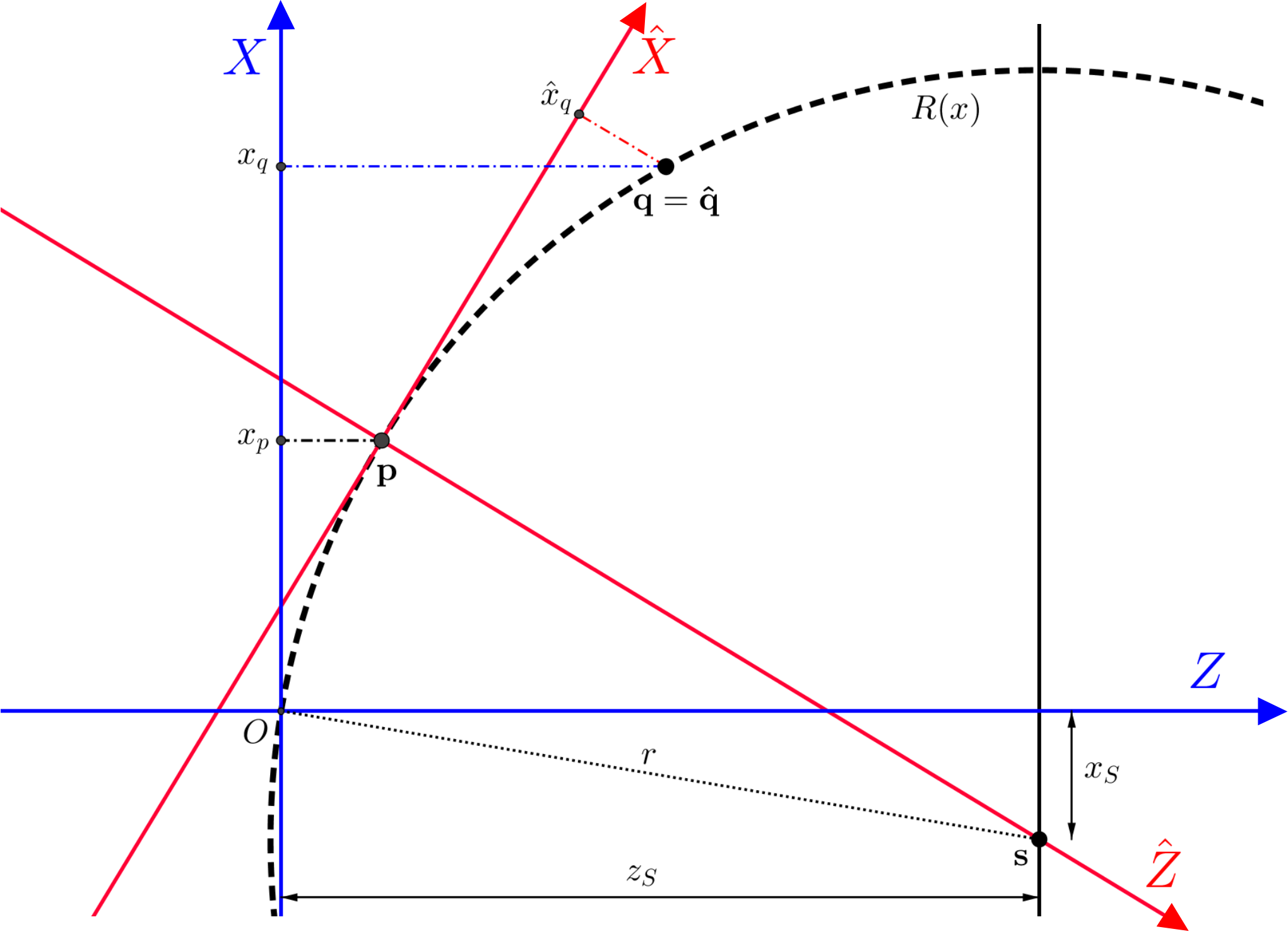
In a local coordinate system, the point has a different set of coordinates . However, the function values of the OPD function in both systems must be the same since and are only different coordinates of the same point, see Fig. 6. We therefore define
| (48) |
where the functions
perform a remapping of the two different parameterizations of the reference sphere. For clarity, we have explicitly denoted the dependence on the evaluation point . For the transfer of functions between the two systems, only the functions and are significant.
The construction above serves as a general tool to transfer all quantities of interest into a local coordinate system, i.e. in addition to the OPD function , the wavefront and the normalized ray direction of the aberrated ray are defined locally via
| (58) |
by linking them to their global definition in exit pupil coordinates.
6 Exact 2D calculation of the wavefront from the wave aberration
6.1 Constructing a Tangent Plane to the Wavefront
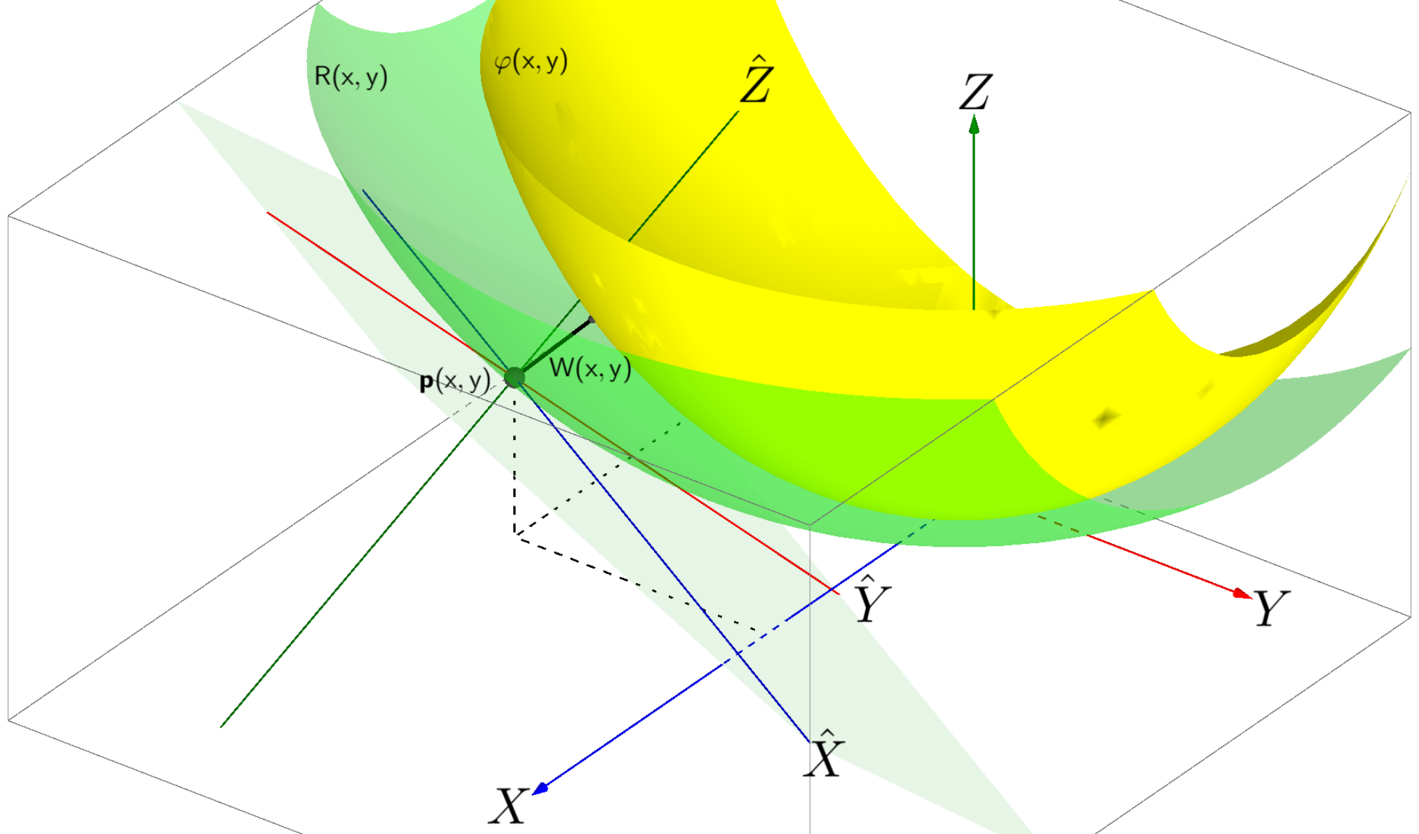
The derivation for the 2D case utilizes the 1D result of Sect. 4 and proceeds along similar lines. To restate the problem: knowing the reference sphere and the OPD function we want to calculate the corresponding wavefront , which is now a function that takes a 2D coordinate to a point in three-dimensional space. According to the wavefront and OPD definitions,
| (59) |
where is again the unknown normalized direction of the aberrated ray and represents the evaluation point on the reference sphere. The derivation is similar to the 1D case, namely the combination of a coordinate transformation and the calculation of a limit. The geometry of the setting as well as the global and local coordinate systems involved are illustrated in Fig. 7.
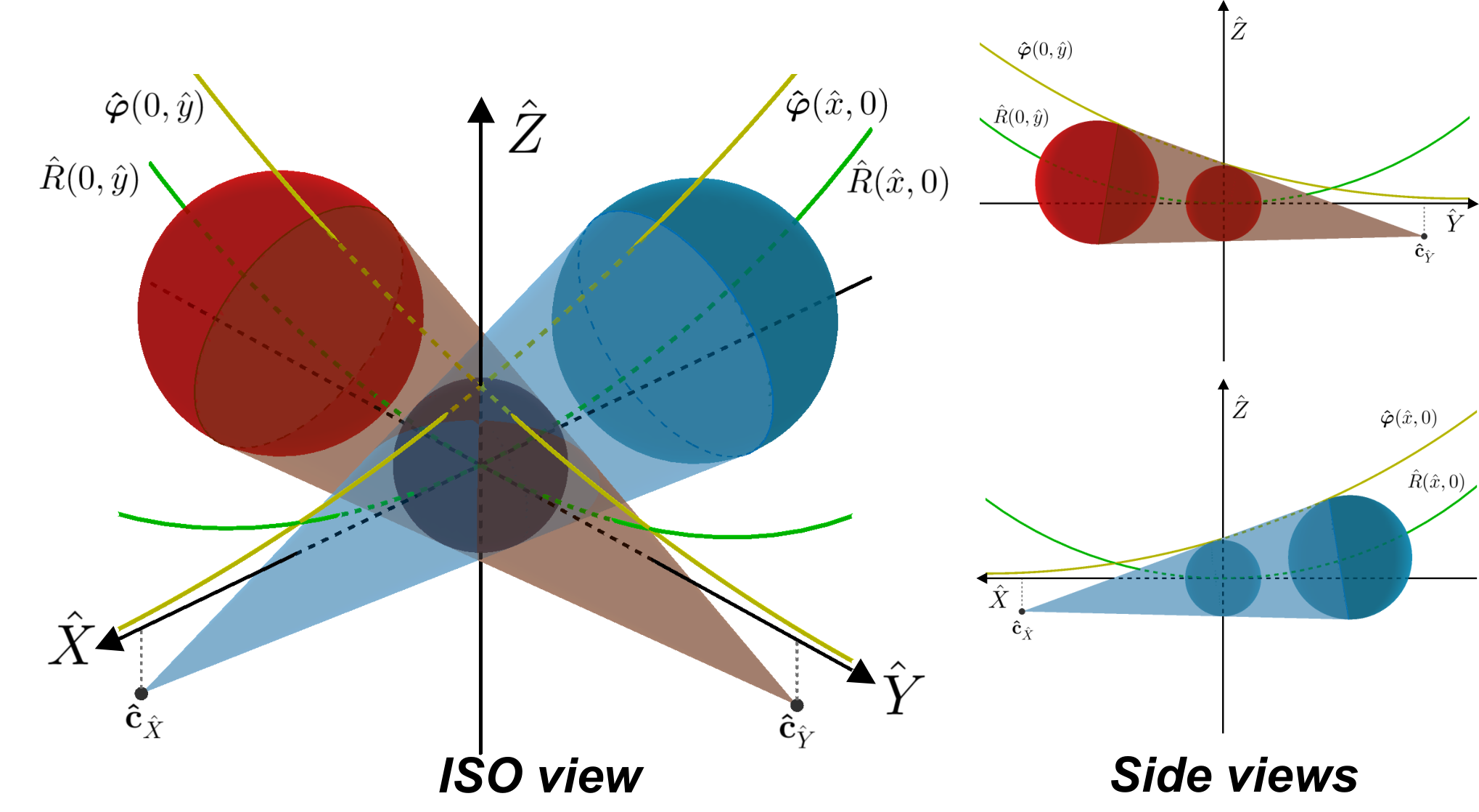
We continue the derivation in local coordinates. We now study two spheres with their centers located on the surface of the reference sphere. Both spheres are tangent to the wavefront. One of them is fixed at the origin of the local coordinate system while the other one approaches it. Ultimately, the two spheres coincide at the limit. Since the second sphere can be approaching from an arbitrary direction, we instead consider two pairs of spheres moving along the local coordinate axes and , respectively. In doing so, we obtain equations where the and components are independent. To each pair of spheres, there is a tangent cone with its vertex located in the and planes respectively.
The two pairs of spheres are illustrated in Fig. 8. In this Figure, the wavefront surface and the reference sphere previously plotted in Fig. 7, are now replaced by single profiles. In the side views we see the two pairs of spheres. The objects tangent to each are now cones with vertices and . Employing the same analysis as in Fig. 5, we find the equations for the coordinates of the vertices.
Consequently, when the spheres are coinciding at the limit, we find the coordinates for the vertices of the cones to be
| (60) |
and
| (61) |
where and represent the distances between centers, along the corresponding axis, for each pair of approaching spheres. The coinciding spheres are shown in Fig. 9. The limit points and are located on the axes and respectively. The tangential circles are located in planes parallel to the and planes.
In the case that either limit approaches infinity, the solution reduces to the 1D case. If both limits are infinite, the wavefront point is at a distance along the axis.
Similar to the 1D case where we obtained the wavefront point using Eqs. (10), we compute the wavefront point as the point of intersection of the limiting tangent circles, as shown in Fig. 9. The and coordinates are obtained using triangle relations as in Fig. 5. The component is determined by observing that both circles in Fig. 9 are part of the limit sphere. The wavefront in the local coordinate system is therefore given by
| (62) |

The normalized ray direction in local coordinates is the vectorial part of the wavefront point and is given by
| (63) |
6.2 Explicit Expressions in Global Coordinates
In the previous sections we have derived equations for the wavefront point and the aberrated ray direction in local coordinates. We now relate them back to the global coordinate system.
Since both the parameters and the values of the functions in Eqs. (62) and (63) are in local coordinates, two steps are necessary:
- 1.
a replacement of local wavefront and wavefront derivative terms by their corresponding expressions in global coordinates, followed by
- 2.
a back-transformation (using Eq. (5.2)) of the still local result into global coordinates.
Before carrying out the two steps, we note that the local OPD function evaluated at the local origin is equal to the global OPD function evaluated at the exit pupil coordinates of point by Eq. (5.2).
Second, the 2D expression for the local wavefront derivatives in global coordinates is
| (64) |
where
| (65) |
with being the elements of the upper left sub-matrix from Eq. (5.1). The relation can be found by differentiating the definition of the function , Eq. (48); the Jacobian of the coordinate transformation, Eq. (5.2), is found to be and Eq. (64) follows by the chain rule. Note that is the transpose of the upper left sub-matrix of and therefore also dependent on .
With these prerequisites we can now perform the transformation in two steps.
Wavefront Point:
Performing step 1 yields
Defining
| (75) |
and performing step 2 yields
which is the 3D wavefront point in global (exit pupil) coordinates as a function of the exit pupil coordinates. Note that the - and -components of will typically not be unless , Eq. (5.2).
Ray Direction:
The aberrated ray direction is similarly transformed into global coordinates. Step 1 results in
| (80) |
Applying step 2, we obtain
| (81) |
Since only three components of the homogeneous direction vector are non-zero, only the upper left matrix of is effective. For general transformations , normals need to be transformed via [10]. In our case, the upper left matrix of is orthonormal and therefore its own inverse transpose.
7 Connection to the ray aberrations
Once the wavefront point and the aberrated ray direction are known, they can be used to compute the transverse ray aberrations. We make a connection to the classical approximation, Eqs. 1, that relates wave and ray aberrations and derive the exact conditions for the approximation to be valid.
The transverse ray aberrations are obtained by computing the aberrated image point and subtracting the paraxial image point from it, i.e.
| (82) |
The aberrated image point is obtained by computing the ray intersection of the aberrated ray with the image plane situated at . The aberrated ray passes, by definition, through the wavefront point , Eq. (6.2), and has the direction , Eq. (81). We compute the path length to the image plane by
| (83) |
where are the components of , the components of , and Eq. (59) has been used. The aberrated image point can now be written as
We see that the point is indeed in the image plane. Using Eq. (82) and ignoring the zero z-component, the transverse ray aberrations become
| (88) |
which, with the help of a computer algebra package, can be simplified to a closed form in terms of the OPD derivative and the paraxial image position :
| (89) |
with
| (90) |
and and . Eqs. (89) are the exact equations of the transverse ray aberrations in terms of the OPD function. We now show that the classic approximation can be obtained as a special case.
Taking the limit as results in
| (91) |
from which we obtain the classical form, Eqs. (1), in the case of . The conditions for the validity of the classical approximation are therefore:
- (i)
the evaluation position in the exit pupil approaches the paraxial image coordinate , and
- (ii)
the gradient norm of the OPD .
It is interesting to note that the best approximation is not obtained in the origin of the exit pupil, but in the exit pupil position closest to the paraxial image.
8 Examples of wavefront and ray aberration calculations
In the following, we provide three representative examples of computations with our analytic expressions. We provide a comparison with results obtained from the classical approximation in Eqs. (1). The comparisons are performed for both the transverse ray aberrations and the reconstructed wavefront. The error between our computation and the classical approximation is studied for all three examples.
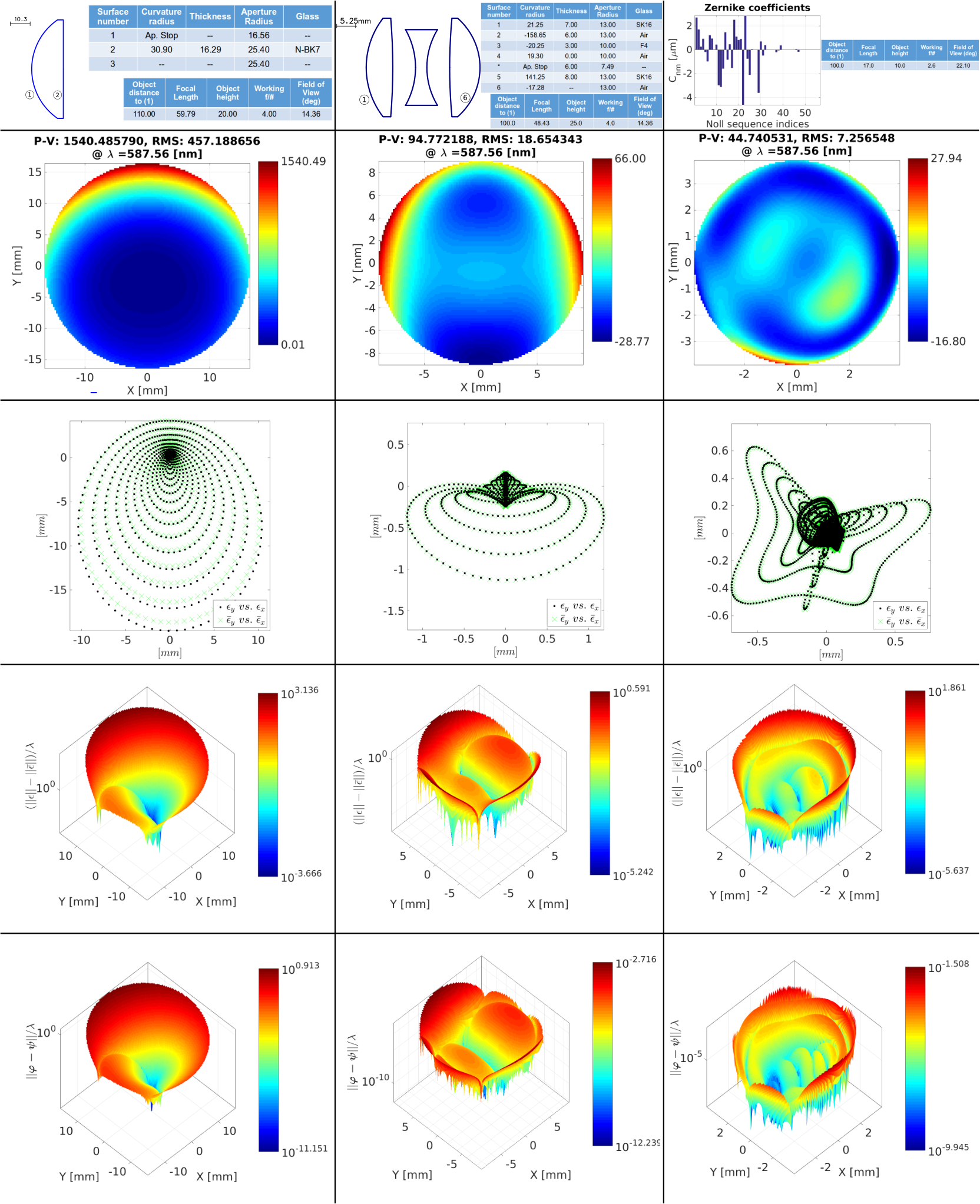
The results are summarized in Fig. 10. Each column is dedicated to a different test case and each row contains the same type of plot for each example. First, we briefly describe the information found in each row and later discuss the results in the context of each of the optical systems.
The first row shows a scaled system diagram, together with the lens prescription and the imaging conditions, reporting all quantities in millimeters. We obtain the first order system properties and a Zernike decomposition of the OPDs from OSLO, a commonly known Optics design software. The number of polynomials for the fit are set to the maximum available, yielding 37 Zernike coefficients. We use the Zernike expansions as ground truth OPD functions, shown in the second row. Additionally, we provide the peak-to-valley (P-V) and RMS values to emphasize the degree of the aberrations.
In the third row we plot the transverse ray aberrations for both directions, which can be considered as a re-centered spot diagram in the paraxial image plane. We simultaneously plot the exact ray aberrations vs. and the classical ray aberrations, now re-named to vs. .
The fourth row presents a comparison between the exact ray aberrations and the classical approximation, by plotting the error in the norms of the transverse ray aberrations , with being the norm of the exact transverse ray aberrations, Eqs. (89), and the norm for the classic equations, Eqs. (1). This surface error is scaled in wavelengths and plotted on a logarithmic axis to enhance its dynamic range.
Finally, the last row presents a comparison of the exactly computed wavefront, Eq. (6.2), with an approximation obtained from the classical equations. For computing the latter, we propose the following procedure: we connect the reference sphere evaluation point with the approximation of the aberrated image point , obtained by adding the classical transverse ray aberrations to the paraxial image point . The direction of this 3D line is an approximation to the true aberrated ray direction , Eq. (81). We use it in conjunction with Eq. (59) to construct an approximated wavefront . The difference in 3D positions is shown in the last row, again scaled in wavelengths and with a logarithmic axis. We include this additional comparison, since the wavefront shape is important for an exact computation of wave-optical point spread functions using Huygens’ principle. We now discuss the individual test cases.
(i) Singlet:
This system is one of the simplest optical set-ups with correspondingly large aberration values, especially at lower f-numbers. We chose a working , focal length at a wavelength . In the OPD plot, a large astigmatic component can be identified, along with a large P-V value. The spot diagram indicates that the classical approximation has a large error for the most external intersection points. The ray aberration error plot further emphasizes this fact, presenting a maximum in the range of . The corresponding wavefront error has a maximum value on the order of .
(ii) Cooke Triplet:
We continue, by studying a more complex and well known system: the Cooke Triplet. The lens prescription is given in the plot. The imaging conditions closely resemble the singlet example, with a working , focal length at a wavelength . The OPD plot indicates a better corrected system, with again a large astigmatic component. The spot diagram indicates that the intersection points from the classical approximation closely resemble the exact calculations. The errors of the classical approximation in both, the ray aberration and the wavefront, are now significantly smaller, with maximum values in the range of and , respectively.
(iii) Post-Surgery Cornea:
We select this example as a test case presenting aberrations of higher order, in contrast to the previous examples where the OPD functions were slowly varying. The Zernike coefficients are extracted from a post-LASIK-surgery corneal topography [11]. In the first row of Fig. 10, we present the list of Zernike coefficients, measured in microns, were the values are listed using the Noll index ordering [12]. To maintain the context of an eye as the optical system, we select a working , focal length at a wavelength . The OPD plot shows a more complex structure giving rise to an unusual spot diagram. The maximum error of the classical approximation in the ray aberrations is now in the order of and the corresponding error for the wavefront comparison has a maximum value on the order of .
Comparing the errors between the cornea and the Cooke triplet examples, we observe the dependence of the approximation error of the classical Eqs. (1) on the derivatives of the wave aberration function. As stated before, Eq. (89), the classical approximation becomes more accurate for smaller gradients of the OPD function. In the post-surgery cornea example, even though the magnitude of the aberrations is smaller than in the Cooke triplet case, we observe approximation errors that are an order of magnitude larger.
9 Conclusions
We have derived exact analytic expressions for the wavefront surface, the aberrated ray directions, and the transverse ray aberrations for the standard definition of the optical path difference as a phase delay along the aberrated ray.
A transition to the local tangent frames of the reference sphere enables a Huygens-like geometric construction of the wavefront as an envelope of spheres and yields additional constraints on the OPD function. We show in the Appendix, that every OPD function satisfying the constraints has an associated wavefront and that the constructed wavefronts and rays fulfill the wavefront properties exactly.
The exact aberrated rays yield exact equations for the transverse ray aberrations. We have identified the precise conditions for the classical approximation to hold. The conditions differ from commonly held assumptions. The relevant factors are small OPD gradients, as opposed to the OPD magnitude, in conjunction with evaluation positions close to the paraxial image coordinates, as opposed to the pupil center.
We presented numerical simulations to illustrate the errors arising from the classical approximation for typical scenarios. The simulations provide a quantitative background for the theoretical results.
Acknowledgments
We thank the anonymous reviewers for their helpful advice and attention to detail. This work has been supported by the German Research Foundation (DFG) through Emmy-Noether grant IH 114/1-1.
Appendix: Validating the Wavefront Properties
We now validate the wavefront properties of the wavefront derived in Eq. (6.2) and the ray direction from Eq. (81). Two conditions must be met for these quantities to be compatible:
The two conditions constitute the definition of a wavefront. In showing that they are met by the quantities in Eqs. (6.2) and (81), we prove their correctness. In addition, the proof also shows that every OPD function, according to the definition of Sect. 3, has a corresponding wavefront.
(i) Wavefront Distance:
We need to show that . For, in this case . Using Eq. (80) in local coordinates, the result is readily obtained:
| (92) | |||||
Since the upper left sub-matrix of transformation is orthonormal, it does not change the length of the normal vector when changing to global coordinates.
∎
(ii) Orthogonality of Wavefront and Aberrated Ray Direction:
We need to show
| (93) |
We proof the equality for the x-tangent vector , the derivation for the y-tangent vector being strictly similar. It is important to perform the proof in global coordinates since the local coordinate system changes when changing the evaluation position .
Denoting the homogeneous local coordinate origin as , the dot-product between the tangent vector and the aberrated ray direction is given by
| (94) | |||||
Simplification of the complete Eq. (94) with a computer algebra package is, unfortunately, not tractable. As indicated above, we decompose the equation into term (I) and term (II). Term (I) will be shown to equal ( for the y-tangent). Term (II) can be shown to equal ( for the y-tangent) with the help of a computer algebra software.
Term :
contributes the majority of cross-terms when multiplying out Eq. (94). It can be conveniently treated in a vectorial fashion:
| (95) | |||||
The last equality is due to the fact that , as shown in Eq. (92), and
| (99) | |||||
The latter equality is due to
which can be verified by multiplying out the expressions.
Term :
is tractable with computer algebra software. Defining
| (104) |
we find that
| (105) |
∎
Summarizing, we have shown that the wavefront point and the aberrated ray directions derived in Sect. 6 are compatible with the wavefront and the OPD properties. Since the proof has been constructive, we have shown that every OPD function according to the definition of Sect. 3 has indeed an associated wavefront.
References
- [1] M. Born and E. Wolf, Principles of Optics (Cambridge University Press, 1999), 7th ed.
- [2] W. Welford, Aberrations of the Symmetrical Optical System (Academic Press, 1974).
- [3] V. N. Mahajan, Optical imaging and aberrations. Part 1. , Ray geometrical optics (SPIE press, Bellingham (Wa.), 1998).
- [4] D. Malacara and Z. Malacara, Handbook of lens design, Optical engineering (Marcel Dekker, New York, 1994).
- [5] J. C. Wyant and K. Creath, Basic Wavefront Aberration Theory for Optical Metrology, Applied Optics and Optical Engineering, Volume XI (Academic Press, 1992).
- [6] B. C. Platt and R. Shack, “History and principles of Shack-Hartmann wavefront sensing.” Journal of Refractive Surgery 17 (2001).
- [7] D. R. Neal, J. Copland, and D. A. Neal, “Shack-hartmann wavefront sensor precision and accuracy,” in “International Symposium on Optical Science and Technology,” (International Society for Optics and Photonics, 2002), pp. 148–160.
- [8] Y. Mejia, “Exact relations between wave aberration and the sagitta difference, and between ray aberration and the slope difference,” Optik - International Journal for Light and Electron Optics 123, 726 – 730 (2012).
- [9] J. Rayces, “Exact relation between wave aberration and ray aberration,” Optica Acta: International Journal of Optics 11, 85–88 (1964).
- [10] A. Glassner and F. Post, “On the transformation of surface normals,” Tech. rep., Faculty of Mathematics and Informatics, Delft University of Technology (1987).
- [11] P. Fricker, “Analyzing lasik optical data using Zernike functions,” MATLAB Digest pp. 1–6 (2008).
- [12] R. J. Noll, “Zernike polynomials and atmospheric turbulence,” J. Opt. Soc. Am. 66, 207–211 (1976).