Subcritical transition to turbulence of a precessing flow in a cylindrical vessel

The experimental setup is illustrated on the Fig. 1. The vessel is a cylinder of radius $R=163$ mm and height $h=326$ mm. It is completely filled with water. For the visualization of the flow (see Fig.2), a small amount of air is introduced. The bubbles are only used to visualize the flow pattern and all the quantitative results have been obtained with a very small amount of bubbles. The container rotates around its symmetry axis. The cylinder is driven by an asynchronous $3$ kW motor via a transmission chain. The power is supplied by a slip ring. To improve the parallelism of the end caps of the cylinder, they are joined together by eight rods (yellow rods on the right Fig.1). The end-cap located at the opposite side of the motor is maintained by a counter bearing, in order to avoid any bending. This structure is mounted on the turntable. It can be tilted to vary the inclination between the direction of the rotation of the cylinder and the direction of the precession. In the present study, the angle is constant at 90^o so that rotation axis and precession axis are orthogonal like in refs [20, 21]. The turntable is driven by a second asynchronous $2.2$ kW motor. The frequency rate of the turntable $f_{t}$ can be increased up to $1$Hz. We have not used a control loop for the motors, in order to avoid perturbations due to the control process, like self excitations, which stress the mechanics of the experiment. The rotation rates of the cylinder and the turntable are continuously measured by two tachometers. The fluctuations of the rotation rates are smaller than $0.05\%$ and the rotation rates do not vary during the transitions from and to the turbulent regime.

We recall all the parameters characterizing our set-up in the table I.

The dimensional analysis allows us to define three dimensionless numbers from the five parameters $(h,R,\nu,\Omega_{c},\Omega_{t})$ (we consider $\Theta$ as a dimensionless number)

We carried out measurements of power consumption at constant Reynolds number $Re=5.65\times 10^{5}$ ($f_{c}=4$Hz). We have performed a first ascending series of measurements from $\epsilon=0$ to $16.4\times 10^{-2}$ and a second descending series from $10\times 10^{-2}$ to $6.56\times 10^{-2}$. Due to the presence of fluctuations at low frequencies (see Fig.3), each measurement lasts $40$ minutes ($9600$ periods) in order to converge the average power consumption $P_{m}(\epsilon)$. The results are reported on Fig. 4.

The average power consumption $P_{m}(\epsilon)$ displays two distinct branches: the lower branch $L$ (squares and circles) with $\epsilon\in[0,\epsilon_{LT}]$ and the turbulent branch $T$ (triangles) with $\epsilon\in[\epsilon_{TL},16\times 10^{-2}]$. The $L$ branch corresponds to the laminar regime (circle) and to the non-linear regime (square). Both branches are disconnected and the system undergoes a subcritical bifurcation from $L$ to $T$ at $\epsilon_{LT}$ and goes back from $T$ to $L$ at $\epsilon_{TL}$. The thresholds are $\epsilon_{LT}=7.3\pm 0.1\times 10^{-2}$ and $\epsilon_{TL}=6.7\pm 0.1\times 10^{-2}$ and the hysteresis is clearly visible with $\epsilon_{LT}-\epsilon_{TL}\simeq 6\times 10^{-3}$ (insert, Fig.4). The determination of $\epsilon_{LT}$ is very robust (section IV.2) whereas a precise measurement of $\epsilon_{TL}$ is very difficult (section V.1).

The behaviour of the power consumption of the $L$ and $T$ branches are quite different. On the $L$ branch, the power consumption does not vary significantly for $\epsilon<0.05$ and increases rapidly between $\epsilon\simeq 0.05$ and $\epsilon_{LT}$. In this range, the resonant triads disappear (section III). The power consumption on the $T$ branch exhibits a linear growth (dashed grey line on Fig.4) with

We performed another series of measurements with constant $\epsilon=8.75\times 10^{↨-2}$ in order to estimate the Reynolds dependence of the power consumption by varying $\Omega_{c}$. The flow remains turbulent for the associated Reynolds numbers, which vary in the range $[3.5,13]\times 10^{5}$. To compare the measurements, we subtract the power consumption at $\epsilon=0$ to remove the mechanical loss (increasing like $\Omega_{c}^{2}$) of the set-up. The power injected in the flow $\Delta P=P_{m}(\epsilon)-P_{m}(0)$ is reported on the left hand side of Fig. 5. It increases like $\Omega_{c}^{3}$ for constant $\epsilon$. The dimensionless power $\Delta P/P_{s}$, with $P_{s}=\rho 2\pi R^{4}L\Omega_{c}^{3}$, is roughly constant for $Re\in[3.5,13]\times 10^{5}$ (right Fig.5), suggesting that the dimensionless injected power becomes independent of the Reynolds number.

From equation 3 and the behaviour shown in Fig. 5, it can be concluded that the power dissipated into the turbulent flow scales like

This scaling differs from the linear viscous theory with $\Delta P/P_{s}\sim\epsilon^{2}Re$ and the theoretical constant bounds, $\Delta P/P_{s}\sim\epsilon^{0}$, expected for large Reynolds numbers and an infinite cylinder [38]. Additional information about the turbulent flow is required to explain the $\epsilon$-dependence of the above scaling law by dimensional analysis.

We have performed a series of measurements to investigate the transition to turbulence at the threshold $\epsilon_{LT}$ at a given Reynolds numbers $Re=5.65\times 10^{5}$. The precession ratio is increased step by step with a plateau time of 60 seconds (240 $f_{c}^{-1}$) and a precession ratio step $\Delta\epsilon=1.42\times 10^{-3}$. We performed $16$ runs with the same procedure, using the pressure signal for the detection of the transition (see left hand side Fig.6 ). The transition always occurs when the precession ratio reaches the value $\epsilon=7.25\times 10^{-2}$. The black curve represents the precession ratio (right ordinate) and the blue curve and the red curve correspond to the pressure signal from the same probe but for two different runs. The pressure can slightly drift due to the thermal expansion of the water but we did not observe any correlation between the drift of the pressure and the onset of the instability, so we believe that this effect does not play any significant role in the dynamics of the flow. We observe at $t_{d}=294$s (resp. $t_{d}=309$s) for the blue (resp. red) curve a drop of the pressure after the growth of the precession ratio to $\epsilon=7.25\times 10^{-2}$ at $t_{p}=280$s. It corresponds to the threshold $\epsilon_{LT}$ for the transition to the turbulence. We have measured the delay $\Delta T=t_{d}-t_{p}$ between the change of $\epsilon$ and the beginning of the instability. The average value of the delay $\Delta T$ is $15$ seconds (60 $f_{c}^{-1}$) with a standard deviation of $9$ seconds ($0.6\times\Delta T$). The delay $\Delta T$ is comparable to the precession period $f_{t}^{-1}=3.3$s and could correspond to the time needed to re-establish the base flow, which then becomes unstable. In any case, the delay $\Delta T$ is much smaller than the typical transient life time of the turbulence in the hysteresis region (see section V).

The discontinuity of the pressure confirms the presence of a subcritical transition. The pressure jump corresponds roughly to $\Delta p\simeq 500$ Pa and is detected simultaneously on the diametrically opposed probes. The transition seems to be global and affects the low frequency components of the pressure field. The pressure drop is likely due to a slowdown of the rotation of the bulk flow. An estimation of this slowdown gives $\Delta f=(\Delta p/\rho)^{1/2}/(2\pi R)\simeq 0.7$ Hz, corresponding to $17.5\%$ of the imposed frequency rate $f_{c}$. The slowdown of the bulk flow in the turbulent regime has also been reported for precessing cylinders [21] and spheres [39].

In order to compare the different realizations, we define a rescaled pressure $\pi$ such that

Now, we investigate the dependence of the threshold as a function of the Reynolds numbers $Re$ . The covered parameter space $(Re,\epsilon)$ is reported on the left hand side of Fig. 7, with $\epsilon_{LT}$ (circle) and $\epsilon_{TL}$ (square). The diamonds represent the frontier between the laminar flow and the non-linear regime. It corresponds to the appearance of free Kelvin modes in the power spectrum (section III). The region between $\epsilon_{LT}$ and $\epsilon_{TL}$ corresponds to the bistable region between the $L$ and the $T$ branch. The threshold $\epsilon_{LT}$ depends weakly on the Reynolds number, following an empirical power law with $\epsilon_{LT}\sim Re^{-0.067}$ (Fig. 7, right). The width of the hysteresis region given by the difference $\epsilon_{LT}-\epsilon_{TL}$, is roughly independent of $Re$.

The turbulent flow exhibits an interesting feature on the range of the hysteresis $\epsilon\in[\epsilon_{TL},\epsilon_{LT}]$. It can suddenly cease and relax to the $L$ branch, with a random lifetime in the turbulent branch. Figure 8 illustrates this phenomenon. The time series of the power consumption for three different runs at $Re=5.65\times 10^{5}$ are displayed on the left hand side. For $t<0$ s, the flow is turbulent with $\epsilon=9.3\times 10^{-2}$ ($>\epsilon_{LT}$) and at $t=0$ s, the rotation rate of the turntable is reduced to $\epsilon=6.84\times 10^{-2}$ with $\epsilon_{TL}<\epsilon<\epsilon_{LT}$. The drop of power consumption corresponds to the transition from the $T$ branch to the $L$ branch. It occurs rapidly after the slowdown for the red curve, or $400$s ($1.6\times 10^{3}f_{c}^{-1}$) for the blue curve. The third realization (black curve) is still turbulent at $t=700$ s ($2.8\times 10^{3}f_{c}^{-1}$). Unlike the resonant collapse [8, 19], the relaxation to the $L$ branch is definitive. We did not observe spontaneous transition from the non-linear regime to the turbulent regime below the threshold $\epsilon_{LT}$.

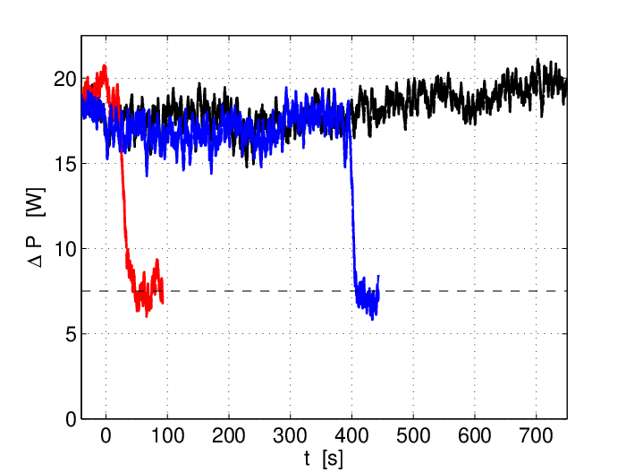
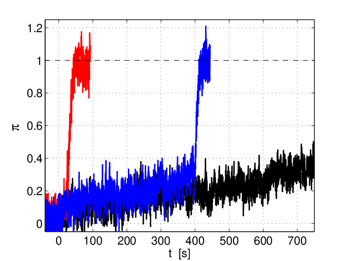
The pressure measurements display also an abrupt transition when the turbulence collapses. The corresponding data are reported on the right side of Fig. 8. The rescaled pressure (defined in section IV.2) suddenly increases at the transition. The dynamics of this relaxation is discussed in section V.3. The turbulence seems to be metastable for a given $\epsilon$ in the hysteresis region $[\epsilon_{TL},\epsilon_{LT}]$. The lifetimes of the turbulence are random and a statistical study of the lifetimes is performed in the next section.

As mentioned in the section IV, the precise determination of $\epsilon_{TL}$ becomes intractable due to the apparent metastability of the hysteresis part of the turbulent branch. We carried out measurements for $\epsilon=6\times 10^{-2}$,i.e. below $\epsilon_{TL}$, with $(\epsilon-\epsilon_{TL})/\epsilon_{TL}\simeq 10\%$. The transition is almost immediate. The delay lasts $10$ s ($40f_{c}^{-1}$) with a small standard deviation of $1.5$ s. This time scale is comparable to the delay $\Delta T$ before the beginning of the transition to turbulence (section IV.2). It turns out that the turbulence is no more metastable for $\epsilon$ smaller than $\epsilon_{TL}$.

The relaxation from the turbulent to the lower branch is a fast process, compared to the transient lifetime of turbulence. We noticed by direct visualization that the turbulent flow still fills the entire vessel (like in the right hand side of Fig.2) before the collapse of the turbulence. We have reported different realizations (in grey) of the relaxation of the pressure $\pi$ on the left of Fig. 11 for $Re=5.65\times 10^{5}$ and $\epsilon=6.7\times 10^{-2}$. The procedure is identical to the one detailed in section IV.2.

All the realizations are concentrated around the average (left hand side of Fig.11, black curve). Unlike the stochastic process of the lifetimes, the relaxation seems to be deterministic with a small variability in the realizations. The transition lasts roughly $20$ seconds. The end of the process ($t>5$s) follows an exponential relaxation with $\pi-1\sim\exp(-\gamma t)$ and $\gamma>0$ (insert in left hand side Fig.11). The relaxation times $\gamma^{-1}$ are reported for different $\epsilon$ on the right of Fig. 11. The parameter $\gamma^{-1}$ is almost constant and stays in the range $[6.5,7.5]$ seconds. For $\epsilon=6\times 10^{-2}$ ($<\epsilon_{TL}$), the relaxation remains also exponential with a similar time scale $\gamma^{-1}=7.69$s, even if the turbulent state is no more metastable in this range of $\epsilon$ (cf section V.1).

In the present study of a precession driven flow, we have confirmed the existence of a subcritical bifurcation to turbulence associated with a discontinuity and a hysteresis. The observed transition to turbulence is a robust process and occurs above a well defined threshold $\epsilon_{LT}$, different from the one of the parametric instability of the forced Kelvin mode. Both the pressure and power consumption measurements exhibit an abrupt variation at the transition from and to turbulence. The behaviour of the power consumption changes at the threshold, with a linear dependence of the power on the precession ratio. The pressure measurements suggest that the transition is associated with a slowdown of the solid body rotation. The threshold $\epsilon_{LT}$ of the transition depends weakly on the Reynolds numbers.

In the region of the hysteresis $\epsilon\in[\epsilon_{TL},\epsilon_{LT}]$, the turbulence can suddenly collapse and lead to a definitive relaminarization of the flow. For a given precession ratio and Reynolds number, the lifetimes $\tau$ of the turbulence are random and are exponentially distributed . The average lifetimes $\langle\tau\rangle$ of the turbulence increase rapidly when $\epsilon$ approaches the threshold $\epsilon_{LT}$ of the sustained turbulence. The growth of the lifetimes $\tau$ is well modelled either by the functional form $\langle\tau\rangle\sim\exp(a|\epsilon-\epsilon_{LT}|^{-\beta})$ with $a$ and $\beta$ positive or an exponential law. A detailed study of the relaxation process shows that the slow component of the pressure follows an exponential function with a relaxation rate weakly dependent of $\epsilon$, even for $\epsilon<\epsilon_{TL}$.

As a conclusion, a schematic bifurcation diagram is presented on the Fig. 12. Three regimes are observed : the laminar and the non-linear regimes on the $L$ branch and the turbulent regime on the $T$ branch (cf section III). The $L$ branch becomes unstable at $\epsilon_{LT}$ and the system undergoes a subcritical bifurcation to turbulence. The flow comes back to the $L$ branch for $\epsilon$ smaller than $\epsilon_{TL}$ (cf section IV). Between $\epsilon_{TL}$ and $\epsilon_{LT}$, the turbulent regime is metastable and exhibits transient lifetimes (cf section V). The sneaking arrow corresponds to the relaxation process to the lower branch. The grey line represents the frontier between the basins of attraction of each branch, even if the turbulence is not strictly speaking an attractor. The collisions between the grey and blue lines (black dots) are only symbolic and do not refer to a saddle-node bifurcation.

The observation of a well-defined threshold $\epsilon_{LT}$ for a sustained turbulence may lead to different conclusions. It could indicate the presence of a linear instability past the onset $\epsilon_{LT}$. The instability could also be triggered by non-normal and non-linear mechanisms. Moreover, if we consider the flow as already chaotic before the instability, the transition could be explained by a crisis[42] of this chaotic set. This bifurcation refers to the collision of the basin of attraction of two chaotic attractors, leading to the emergence of only one attractor. However, a non-linear instability is not consistent with the measured robustness of the threshold, whereas the crisis would be associated with random waiting times before the transition. The linear instability is thus the best candidate for the transition to turbulence. As the instability of the laminar flow occurs for smaller precession ratios than $\epsilon_{LT}$, the mechanism of this new instability could differ from the parametric instability of the Kelvin modes [16].